Survival Probabilities for High Mass Diffraction

Abstract:

Based on the calculation of survival probabilities, we suggest a procedure to assess the value of $G_{3P}$, the triple Pomeron ’bare’ coupling constant, by comparing the large rapidity gap single high mass diffraction data in proton-proton scattering and $J/\Psi$ photo and DIS production. For $p$-$p$ scattering the calculation in a three amplitude rescattering eikonal model, predicts the survival probability to be an order of magnitude smaller than for the two amplitude case. The calculation of the survival probabilities for photo and DIS $J/\Psi$ production are made in a dedicated model. In this process we show that, even though its survival probability is considerably larger than in $p$-$p$ scattering, its value is below unity and cannot be neglected in the data analysis. We argue that, regardless of the uncertainties in the suggested procedures, the outcome is important, both with regards to a realistic estimate of $G_{3P}$, and the survival probabilities relevant to LHC experiments.

1 Introduction

A large rapidity gap (LRG) process is defined as one where no hadrons are produced in a sufficiently large rapidity interval. Diffractive LRG are assumed to be produced by the exchange of a color singlet object with quantum numbers of the vacuum, which we will refer to as the Pomeron. We wish to estimate the probability that a LRG, which occurs in diffractive events, survives rescattering effects which populate the gap with secondary particles coming from the underlying event.

At high energies, elastic and inelastic diffractive processes account for about $40\%$ of the total $p$-$p$ ($\bar{p}$-$p$) cross section. We would like to remind the reader that:

1. The small $t$ behavior of the scattering amplitude is determined, mostly, by the large impact parameter $b$ values.

2. The survival probability $<|S|^{2}>$ (denoted $S^{2}$) of a diffractive LRG is obtained from a normalized convolution of the b-space diffractive amplitude squared and $e^{-\Omega(s,b)}$. ${\Omega(s,b)}$ is the optical density, also called opacity. Consequently, $S^{2}$ decreases with increasing energy due to the growth with energy of the interaction input opacity.

3. $S^{2}$ is not only dependent on the probability of the initial state to survive, but is also sensitive to the spatial distribution of the partons inside the incoming hadrons and, thus, on the dynamics of the whole diffractive part of the scattering matrix.

4. $S^{2}$, at a given energy, is not universal. It depends on the particular diffractive subprocess, as well as the kinematic configurations. It also depends on the nature of the color singlet (P, W/Z or $\gamma$) exchange which is responsible for the LRG.

Historically, both Dokshitzer et al.[1] and Bjorken[2] suggested utilizing a LRG as a signature for Higgs production originating from a W-W fusion sub-process, in hadron-hadron collisions. It turns out that LRG processes give a unique opportunity to measure the high energy asymptotic behavior of the amplitudes at short distances, where one can calculate the amplitudes using methods developed for perturbative QCD (pQCD). Consider a typical LRG process - the production of two jets with large transverse momenta $\vec{p}_{t1}\,\,\approx\,\,-\vec{p}_{t2}\,\,\gg\,\,\mu$, with a LRG between the two jets. $\mu$ is a typical mass scale of the soft interactions.

$$p(1)\,\,+\,\,p(2)\,\,\longrightarrow\,\,M_{1}[hadrons\,\,+\,\,jet_{1}(y_{1},p_{t1})]$$ (1.1)

$$+\,\,LRG[\Delta y=|y_{1}-y_{2}|]\,\,+\,\,M_{2}[hadrons\,\,+\,\,jet_{2}(y_{2},p_{t2})].$$

$y_{1}$ and $y_{2}$ are the rapidities of the jets and $\Delta y\,\,\gg\,\,1$. The production of two hard jets with a LRG is initiated by the exchange of a hard Pomeron. We define $F_{s}$ to be the ratio between the cross section due to the above Pomeron exchange, and the inclusive inelastic cross section with the same final state generated by gluon exchange. In QCD we do not expect this ratio to decrease as a function of the rapidity gap $\Delta y$. For a BFKL Pomeron[3], we expect an increase once $\Delta y\,\gg\,\,1$. Using a simple QCD model for the Pomeron, in which it is approximated by two gluon exchange[4], Bjorken[2] gave the first estimate for $F_{s}\,\approx\,\,0.15$, which is unexpectedly large.

As noted by Bjorken[2] and GLM[5], one does not measure $F_{s}$ directly in a LRG experiment. The experimentally measured ratio between the number of events with a LRG, and the number of similar events without a LRG is not equal to $F_{s}$, but, has to be modified by an extra suppression factor which we call the LRG survival probability,

$$f_{gap}=<\mid S\mid^{2}>\times F_{s}\,.$$ (1.2)

The appearance of $S^{2}$ in Eq. (1.2) has a very simple physical interpretation. It is the probability that the LRG due to Pomeron exchange, will not be filled by the produced particles (partons and/or hadrons) from the rescattering of the spectator partons, or from the emission of bremsstrahlung gluons coming from the partons, or the hard Pomeron, taking part in the hard interaction.

$$<\mid S\mid^{2}>\,\,=\,\,<\mid S_{bremsstrahlung}(\Delta y\,=\,|\,y_{1}\,-\,y_{2}\,|)\mid^{2}>\times<\mid S_{spectator}(\,s\,)\mid^{2}>\,,$$ (1.3)

where $s$ denotes the total c.m. energy squared.

• $S_{bremsstrahlung}^{2}(\Delta y)$ can be calculated in pQCD[6]. It depends on the kinematics of each specific process, and on the value of the LRG . This suppression is commonly included in the calculation of the hard LRG sub process.

• To calculate $S_{spectator}^{2}(s)$ we need to find the probability that all partons with rapidity $y_{i}\,>\,y_{1}$ in the first hadron, and all partons with $y_{j}\,<\,y_{2}$ in the second hadron, do not interact inelastically and, hence, do not produce additional hadrons within the LRG interval. This is a difficult problem, since not only partons at short distances contribute to such a calculation, but also partons at long distances, for which the pQCD approach is not valid. Many attempts have been made to estimate $S_{spectator}^{2}$[2, 5, 7, 8, 9, 10, 11], but a unique solution, has still not been found.

An obvious check of the above is to compare the calculated values of $S^{2}_{spectator}(s)$ obtained in different models for different reactions. The Durham group[12] recently suggested a very interesting procedure, proposing to extract $G_{3P}$, the triple Pomeron vertex coupling, utilizing the measurement of large mass diffraction dissociation in the reaction

$$\gamma^{*}(Q^{2},x_{Bj})\,+\,p\,\Longrightarrow\,J/\Psi\,+\,[LRG]\,+\,X(M^{2}\gg\ m_{p}).$$ (1.4)

The cross section of this process can be described by the Mueller diagram (Fig. 2). It is initiated by the charm component of the photon which has a small absorptive cross section, since its interaction stems from short distances ($r\propto 1/m_{c}$, where $m_{c}$ is the mass of the charm quark). Thus, the probability for additional rescatterings (Fig. 2) is relatively small, resulting in a high survival probability. This is to be compared with the corresponding high mass diffraction in an hadronic $p$-$p$ ($\bar{p}$-$p$) reaction (Fig. 4), for which we expect the rescatterings (Fig. 4) to be significant, resulting in a small survival probability[13]. It is, therefore, very probable that present extractions[14, 15] of the 3P coupling are underestimated. Comparing the values of $G_{3P}$ obtained in the above two channels, taking into account their (different) survival probabilities, leads to a more reliable measure of the 3P coupling, and provides a check of the various theoretical estimates of the survival probabilities.

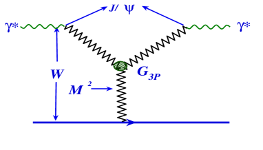
Figure 1: The general diagram for diffractive production of large masses in $\gamma^{*}$-$p$ collisions at high energy. Pomerons are denoted by the zigzag lines. The vertical lower Pomeron is soft. The two Pomerons coupled to the photon vertices are hard.

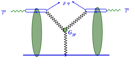
Figure 2: The general diagram for calculating the survival probability for diffractive production of large masses in $\gamma^{*}$-$p$ collisions at high energy. The Pomerons identification is identical to the previous figure.

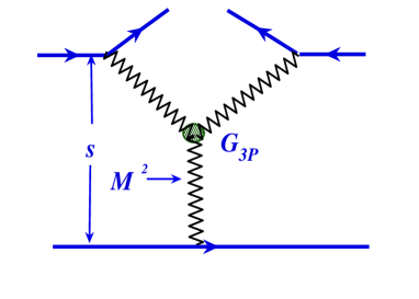
Figure 3: The general diagram for diffractive production of large masses in $p$-$p$ collisions at high energy. The zigzag lines denote soft Pomerons.

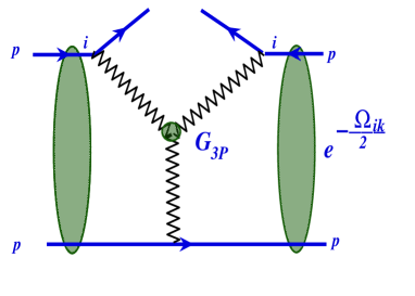
Figure 4: The general diagram for calculating the survival probability for diffractive production of large masses in $p$-$p$ collisions at high energy. The zigzag lines denote soft Pomerons.

The purpose of this paper is to re-examine the procedure to extract the value of $G_{3P}$, the triple Pomeron ’bare’ coupling constant. As a by-product we assess the stability of the survival probabilities obtained in two and three amplitude eikonal rescattering models. The following topics are addressed:

1. We estimate the survival probability values for the triple Pomeron vertex in $p$-$p$ high mass single diffractive (SD) collisions.

2. We investigate the difference between the survival probabilities associated with high mass SD and the inclusive SD channels.

3. The above calculations are carried out in the two channel GLM model[16, 17, 18] in which we compare the output of its two and three amplitude representations, so as to assess the reliability of our results.

4. We calculate the survival probability for the reaction given by Eq. (1.4). Note that in an hadronic high mass SD reaction the 3P coupling consists of three soft Pomerons. Eq. (1.4) is a hard process in which two hard Pomerons couple to a soft one. It is possible, but not necessary, that the above 3P couplings are equal.

The plan of our paper is as follows: In the next section we calculate $S^{2}_{spectator}(s)$ for high mass diffraction in $p$-$p$ scattering in two[16] and three[17] amplitude models for the soft interactions. The models are specified and their outputs compared. In section 3 we present our estimates for the survival probability of the process of Eq. (1.4). These calculations, carried out in a dedicated model[19], show that even though the $J/\Psi$ survival probabilities are significantly larger than those calculated for $p$-$p$, they cannot be neglected. We note that, the reliability and accuracy of the $J/\Psi$ calculations are considerably better than in the $p$-$p$ channel. In the conclusions, we summarize our main results and specify some remaining problems.

2 Survival probability for the triple Pomeron vertex in proton-proton collisions

2.1 Survival probability in the eikonal model

The cross section for diffractive dissociation in the region of large $M$ can be viewed as a Mueller diagram (Fig. 4) which can be rewritten in terms of the triple Pomeron vertex (see Ref.[14]). We denote this cross section $\sigma^{3P}$ and its corresponding survival probability, at a given $M^{2}$, $S^{2}_{3P}(M^{2})$.

$$M^{2}\,\frac{d\sigma^{3P}}{dt\,dM^{2}}\,\,\,=\,\,\,\frac{g^{2}_{p}(t)\,g_{p}(q^{2}=0)\,G_{3P}(t)}{16\,\pi^{2}}\,\,\left(\frac{s}{M^{2}}\,\right)^{2\alpha_{P}(t)-2}\,\left(\,\frac{M^{2}}{s_{0}}\right)^{\alpha_{P}(q^{2}=0)-1},$$ (2.5)

where $g(t)$ describe the vertex of Pomeron-proton interaction, and $G_{3P}$ stands for the triple Pomeron vertex. However, this diagram does not take into account the possibility of additional rescatterings of the interacting particles shown in Fig. 4. The result can be written as

$$M^{2}\,\frac{d\sigma^{3P}}{dt\,dM^{2}}\,=\,S^{2}_{3P}(M^{2})\,\,\frac{g^{2}_{p}(t)\,g_{p}(q^{2}=0)\,G_{3P}(t)}{16\,\pi^{2}}\,\,\left(\frac{s}{M^{2}}\,\right)^{2\alpha_{P}(t)-2}\,\left(\,\frac{M^{2}}{s_{0}}\right)^{\alpha_{P}(q^{2}=0)-1}.$$ (2.6)

The survival probability factor $S^{2}_{3P}(M^{2})$ is defined as

$$S^{2}_{3P}(M^{2})\,\,=\,\,\frac{\int\,d^{2}\,k_{t}\,\,M^{2}\,\frac{d\sigma^{3P}}{d\,k^{2}_{t}\,dM^{2}}\left({Fig.~{}\ref{3pspdia}}\right)}{\int\,d^{2}\,k_{t}\,\,M^{2}\,\frac{d\sigma^{3P}}{d\,k^{2}_{t}\,dM^{2}}\left({Fig.~{}\ref{3pdia}}\right)}\,\,\,,\,\,\,\,\,\,\,\,\,\mbox{with}\,\,\,\,t\,=\,\,-\,k^{2}_{t}.$$ (2.7)

The easiest way to calculate the diagram of Fig. 4 is to first transform the diagram of Fig. 4 to impact parameter space. This is done by introducing the momentum $q$ along the lowest Pomeron in Fig. 4. In this case,

$$T\left(s,M^{2};q\right)\,\,\equiv\,\,\int\,d^{2}\,k_{t}\,\,M^{2}\,\frac{d\sigma^{3P}}{dk^{2}_{t}\,dM^{2}}\left({Fig.~{}\ref{3pdia}}\right)\,\,\,\longrightarrow\,$$ (2.8)

$$\int\,d^{2}k_{t}\,\,\frac{g_{p}(k^{2}_{t})\,g_{p}((\vec{k}-\vec{q})^{2}_{t})\,g_{p}(q^{2}_{t})\,G_{3P}(k^{2}_{t},(\vec{k}-\vec{q})^{2}_{t},q^{2})}{16\,\pi^{2}}\,\,\left(\frac{s}{M^{2}}\,\right)^{\alpha_{P}(k^{2}_{t})\,+\,\alpha_{P}((\vec{k}-\vec{q})^{2}_{t})\,-\,2}\,\left(\,\frac{M^{2}}{s_{0}}\right)^{\alpha_{P}(q^{2})-1}\,.$$

From Eq. (2.8) we find the form of this amplitude in impact parameter space to be

$$T\left(s,M^{2};b\right)\,\,\equiv\,\,\int\,\frac{d^{2}q}{(2\pi)^{2}}\,\,A\left(s,M^{2};q\right).$$ (2.9)

Using a linear approximation for the Pomeron trajectory and a Gaussian form for all vertices

$$\alpha_{P}(t)=1\,+\,\Delta\,\alpha^{\prime}_{P}\,t,\,\,\,\,\,\,g_{p}(k^{2})=g_{p}(0)\,e^{-b_{p}\,k^{2}},\,\,\,\,\,\,G_{3P}(k_{1},k_{2},k_{3})=G_{3P}(0,0,0)\,e^{-b_{p}(k^{2}_{1}\,+\,k^{2}_{2}\,+\,k^{2}_{3})}\,,$$ (2.10)

we obtain

$$T\left(s,M^{2};b\right)\,=\,\frac{g_{3P}}{16\pi^{2}}\,\nu(\xi)\,\nu(\xi)\,\nu(y)\,\frac{\pi}{d(\xi)+d(\xi)+d(y)}\,\exp\left(-\frac{d(y)\,[d(\xi)+d(\xi)]}{d(\xi)+d(\xi)+d(y)}\,b^{2}\right).$$ (2.11)

$$y\,=\,\ln\left(M^{2}/s_{0}\right),\,\,\,\,\,\,\xi\,=\,\ln\left(s/M^{2}\right),\,\,\,\,\,\,g_{3P}\,\,\equiv\,\,G_{3P}(0,0,0)/g_{p}(0),\,\,\,\,\,\,\nu(y)\,=\,\frac{g^{2}_{p}(0)}{\pi\bar{R}^{2}(y)}\,e^{\Delta\,y},$$ (2.12)

where

$$\bar{R}^{2}(y)\,\,=\,\,2\,R^{2}_{0}\,\,+\,\,2\,r^{2}_{0}\,+\,4\,\alpha^{\prime}_{P}\,y\,\,\,\,\,\,\mbox{and}\,\,\,\,\,\,d(y)\,\equiv\,\frac{1}{\bar{R}^{2}(y)}.$$ (2.13)

$r^{2}_{0}$ denotes the radius of the triple Pomeron vertex. In the following we take [20] $r^{2}_{0}\,=\,0.5\,GeV^{-2}$.

Using Eq. (2.11), the expression for the survival probability (see Eq. (2.7)) in a simple eikonal model, accounting for the rescattering corrections, can be written as

$$S^{2}_{3P}(M^{2})\,=\,\frac{\int\,d^{2}b\,T\left(s,M^{2};b\right)\,\exp\left(\,-\,\Omega\left(\xi+y;b\right)\,\right)}{\int\,d^{2}b\,T\left(s,M^{2};b\right)},\,\,\,\,\,\mbox{where}\,\,\,\,\,\Omega\left(\xi+y;b\right)\,=\,\nu_{pp}\,e^{-\frac{b^{2}}{R_{pp}(\xi+y)}}.$$ (2.14)

$$\nu_{pp}\,=\,\frac{g^{2}_{p}(0)}{\pi R_{pp}(\xi+y)}\,e^{\Delta(\xi+y)}\,\,\,\,\,\mbox{and}\,\,\,\,\,R_{pp}(\xi+y)\,=\,4\,R^{2}_{0,p}\,+\,4\,\alpha^{\prime}_{P}\,(\xi y).$$ (2.15)

2.2 Two channel models: main ideas and formulae

In the eikonal model only elastic rescatterings have been taken into account. Two channel eikonal models have been developed so as to also include rescatterings through diffractive dissociation (see Refs.[16, 17, 18] and references therein). In this formalism, diffractively produced hadrons at a given vertex are considered as a single hadronic state described by the wave function $\Psi_{D}$, which is orthonormal to the wave function $\Psi_{h}$ of the hadron (proton in the case of interest), $<\Psi_{h}|\Psi_{D}>\,=\,0$.

Introducing two wave functions that diagonalize the 2x2 interaction matrix ${\bf T}$

$$A_{i,k}\,=\,<\Psi_{i}\,\Psi_{k}|\mathbf{T}|\Psi_{i^{\prime}}\,\Psi_{k^{\prime}}>\,\,=\,\,A_{i,k}\,\delta_{i,i^{\prime}}\,\delta_{k,k^{\prime}},$$ (2.16)

In our past publications we referred to the GLM eikonal models according to the number of the rescattering channels considered, i.e. elastic[20], elastic + SD[16] and elastic + SD + DD[17]. In retrospect, we consider it more appropriate to define these models according to the dimensionality of their base. We, therefore, call the above a two channel model, making the distinction between its two and three amplitude representations.

We can rewrite the amplitude $A_{i,k}$ in a form that satisfies the unitarity constraints

$$A_{i,k}(s,b)\,=\,i\,\left(\,1\,-\,\exp\left(-\frac{\Omega_{i,k}(s,b)}{2}\right)\right).$$ (2.17)

In this formalism we have

$$G^{in}_{i,k}(s,b)\,=\,1\,-\,\exp\left(-\Omega_{i,k}(s,b)\right).$$ (2.18)

$G^{in}$ is the probability for all inelastic interactions in the scattering of particle $i$ off particle $k$. From Eq. (2.18) we deduce that the probability that the initial projectiles reach the interaction unchanged, regardless of the initial state rescatterings, is $\exp\left(-\Omega_{i,k}(s,b)\right)$.

In this representation the observed states can be written in the form

$$\Psi_{h}\,=\,\alpha\,\Psi_{1}\,+\,\beta\,\Psi_{2}\,,\,\,\,\,\,\,\,\,\Psi_{D}\,=\,-\,\beta\,\Psi_{1}\,+\,\alpha\,\Psi_{2}\,,\,\,\,\,\,\,\,\,\mbox{where}\,\,\,\,\,\,\,\alpha^{2}\,+\,\beta^{2}\,\,=\,\,1.$$ (2.19)

The obvious generalization of Eq. (2.11) is

$$T\left(s,M^{2};b\right)\,=\,\sum_{i,k,l}\,<p|l>^{2}\,<p|k>\,T^{l,i}_{k}\left(s,M^{2};b\right)\,<p|k>\,<p|i>^{2},$$ (2.20)

where $<p|1>\,=\,\alpha$ and $<p|2>\,=\,\beta$.

$$T^{l,i}_{k}\left(s,M^{2};b\right)\,=\,\frac{g_{3P}}{16\pi^{2}}\,\nu_{l}(\xi)\,\nu_{i}(\xi)\,\nu_{k}(y)\,\frac{\pi}{d_{l}(\xi)+d_{i}(\xi)+d_{k}(y)}\,\exp\left(-\frac{d_{k}(y)\,[d_{l}(\xi)+d_{i}(\xi)]}{d_{l}(\xi)+d_{i}(\xi)+d_{k}(y)}\,b^{2}\right),$$ (2.21)

where $g_{3P}\,=\,G_{3P}/g_{1}(0)$ and

$$\nu_{k}(y)\,=\,\frac{g_{k}(0)g_{1}(0)}{\pi\bar{R}^{2}_{k}(y)}\,e^{\Delta\,y}\,\, \,\bar{R}^{2}_{k}(y)\,=\,2\,R^{2}_{0,k}\,+\,2\,r^{2}_{0}\,+\,4\,\alpha^{\prime}_{P}\,y,\,\,\,\,\,\,d_{k}(y)\,\equiv\,\frac{1}{\bar{R}^{2}_{k}(y)}\,.$$ and (2.22)

The numerator of Eq. (2.14) is written in this representation as

$$\int d^{2}\,k_{t}\,M^{2}\,\frac{d\sigma^{3P}}{dk^{2}_{t}\,dM^{2}}\left({Fig.~{}\ref{3pspdia}}\right)\,=$$ (2.23)

$$\,\,\int\,d^{2}b\,\sum_{i,k,l}\,<p|l>^{2}\,<p|k>\,e^{-\frac{\Omega_{l,k}(s,b)}{2}}\,\,T^{l,i}_{k}\left(s,M^{2};b\right)\,e^{-\frac{\Omega_{i,k}(s,b)}{2}}\,<p|k>\,<p|i>^{2}.$$

For $\Omega_{i,k}(s,b)$ we take

$$\Omega_{i,k}(s,b)\,=\,\nu_{i,k}\,e^{-\frac{b^{2}}{R^{2}_{i,k}(\xi+y)}}\,,$$ (2.24)

where

$$\nu_{i,k}\,=\,\frac{g_{i}(0)\,g_{k}(0)}{\pi\,R^{2}_{i,k}(\xi+y)}\left(\frac{s}{s_{0}}\right)^{\Delta},\,\,\,\,\ \mbox{and}\,\,\,\,\,R^{2}_{i,k}(\xi+y)\,=\,2\,R^{2}_{0,i}+2\,R^{2}_{0,k}\,+\,4\,\alpha^{\prime}_{P}\,(\xi+y)\,.$$ (2.25)

In the following we denote $g^{2}_{i,k}\,=\,g_{i}(0)g_{k}(0)$.

In our calculations we take [16] $R^{2}_{0,1}$ as a free parameter while $R^{2}_{0,2}=0$. The survival probability can be calculated as the ratio

$$S^{2}_{3P}(M^{2})\,=\,\frac{\int\,d^{2}\,b\,\,N(\xi,y;b)}{\int\,d^{2}\,b\,\,D(\xi,y;b)},$$ (2.26)

where

$$N(\xi,y;b)\, = \,\alpha^{6}\,T^{1,1}_{1}(b)\,e^{-\Omega_{1,1}(b)}\,+\,2\,\alpha^{4}\,\beta^{2}\,T^{1,2}_{1}(b)\,e^{-\frac{\Omega_{1,1}(b)+\Omega_{1,2}(b)}{2}}\,+\,\alpha^{2}\,\beta^{4}\,T^{2,2}_{1}(b)\,e^{-\Omega_{1,2}(b)}$$ (2.27)

$$+\,\alpha^{4}\,\beta^{2}\,T^{1,1}_{2}(b)\,e^{-\Omega_{1,2}(b)}\,+\,2\,\alpha^{2}\,\beta^{4}\,T^{1,2}_{2}(b)\,e^{-\frac{\Omega_{2,2}(b)+\Omega_{1,2}(b)}{2}}\,+\,\beta^{6}\,T^{2,2}_{2}(b)\,e^{-\Omega_{2,2}(b)}\,,$$

and

$$D(\xi,y;b)\, = \,\alpha^{6}\,T^{1,1}_{1}(b)\,+\,2\,\alpha^{4}\,\beta^{2}\,T^{1,2}_{1}(b)\,+\,\alpha^{2}\,\beta^{4}\,T^{2,2}_{1}(b)\,\,$$ (2.28)

$$\,+\,\alpha^{4}\,\beta^{2}\,T^{1,1}_{2}(b)\,+\,2\,\alpha^{2}\,\beta^{4}\,T^{1,2}_{2}(b)\,+\,\beta^{6}\,T^{2,2}_{2}(b)\,.$$

For completeness we also present the integrated cross sections of the diffractive channels in the two channel model, together with the corresponding elastic and total cross sections. The amplitudes for the elastic and the diffractive channels have the following form [16, 17]

$$a_{el}\left(s,b\right)\, = \,i\,\left(\,1\,-\alpha^{4}\,e^{-\frac{\Omega_{1,1}(s,b)}{2}}\,-\,2\,\alpha^{2}\,\beta^{2}\,e^{-\frac{\Omega_{1,2}(s,b)}{2}}\,-\,\beta^{4}\,e^{-\frac{\Omega_{2,2}(s,b)}{2}}\right),$$ (2.29)

$$a_{sd}\left(s,b\right)\, = \,i\,\alpha\,\beta\left(\,\,\alpha^{2}\,e^{-\frac{\Omega_{1,1}(s,b)}{2}}\,-\,(\alpha^{2}\,-\,\beta^{2})\,e^{-\frac{\Omega_{1,2}(s,b)}{2}}\,-\,\,\beta^{2}\,e^{-\frac{\Omega_{2,2}(s,b)}{2}}\,\right),$$ (2.30)

$$a_{dd}\left(s,b\right)\, = \,i\,\alpha^{2}\,\beta^{2}\left(\,-\,e^{-\frac{\Omega_{1,1}(s,b)}{2}}\,+\,2\,e^{-\frac{\Omega_{1,2}(s,b)}{2}}\,-\,e^{-\frac{\Omega_{2,2}(s,b)}{2}}\,\right).$$ (2.31)

Using Eq. (2.24) and Eq. (2.25), as well as the general cross section formulae we get

$$\sigma_{tot}(s)\,=\,2\int\,d^{2}b\,a_{el}\left(s,b\right),\,\,\,\,\,\,\sigma_{el}(s)\,=\,\int\,d^{2}\,b\,\,|a_{el}\left(s,b\right)|^{2},$$ (2.32)

$$\sigma_{sd}(s)\,=\,\int\,d^{2}\,b\,|a_{sd}\left(s,b\right)|^{2},\,\,\,\,\,\,\sigma_{dd}(s)\,=\,\int\,d^{2}\,b\,|a_{dd}\left(s,b\right)|^{2}.$$ (2.33)

It is instructive to present the calculation for the diffractive channels in the form of a survival probability, which we define as the ratio of the output corrected diffractive cross section to the input non corrected cross section.

$$S^{2}_{sd}\,=\,\frac{\int\,d^{2}\,b\,|a_{sd}(s,b)|^{2}}{\int\,d^{2}\,b\,|a^{1}_{sd}(s,b)|^{2}}\,,$$ (2.34)

where

$$a^{1}_{sd}\left(s,b\right)\,=\,\frac{i\,\alpha\,\beta}{2}\left(-\,\alpha^{2}\,\Omega_{1,1}(s,b)\,+\,(\alpha^{2}\,-\,\beta^{2})\,\Omega_{1,2}(s,b)\,+\,\beta^{2}\,\Omega_{2,2}(s,b)\right).$$ (2.35)

We will discuss the results and interpretation of our calculations in the next subsection.

2.3 Three models used for fitting the experimental data

To calculate the survival probabilities one needs to specify the opacities $\Omega_{i,k}(s,b)$. These are determined from a global fit of the experimental soft scattering data. We have used three models based on the general formulae given in Eq. (2.21) - Eq. (2.25), but with different input assumptions. Note that the above global fit has in addition to the Pomeron contribution, also a secondary Regge sector (see Ref.[16]). This is necessary as the data base contains many experimental points from lower ISR energies. A study of the Pomeron component alone, without a Regge contribution, is not possible at this time, since the corresponding high energy sector of the data base is too small to constrain the fitted parameters. The Regge parameters are not quoted in this paper and will be discussed in detail in a forthcoming publication.

2.3.1 Two amplitude model

In this model, denoted by Model A [16] we assume that the double diffraction cross section is negligible, and we take $a_{dd}$ in Eq. (2.31) to be zero. This allows us to express $\Omega_{2,2}$ in terms of $\Omega_{1,1}$ and $\Omega_{1,2}$, leading to the following formulae (see Refs.[16, 17, 18]):

$$a_{el}(s,b)\,=\,i\left(1-\exp\left(-\frac{\Omega_{1,1}(s,b)}{2}\right)-\,2\,\beta^{2}\,\exp\left(-\frac{\Omega_{1,1}(s,b)}{2}\right)\,\left(1\,-\,\exp\left(-\frac{\Delta\Omega(s,b)}{2}\right)\right)\right),$$ (2.36)

$$a_{sd}(s,b)\,=\,-i\,\alpha\,\beta\,\exp\left(-\frac{\Delta\Omega(s,b)}{2}\right)\,\left(1\,-\,\exp\left(-\frac{\Delta\Omega(s,b)}{2}\right)\right)\,.$$ (2.37)

The above is a two amplitude model with two opacities $\Omega_{1,1}$ and $\Delta\Omega\,=\,\Omega_{1,2}\,-\,\Omega_{1,1}\,.$ Following Ref.[16], we assume both $\Omega_{1,1}$ and $\Delta\Omega$ to be Gaussian in b.

$$\Omega_{1,1}(s,b)\,=\,\frac{g^{2}_{1,1}}{\pi R^{2}_{1,1}(s)}\,\left(\frac{s}{s_{0}}\right)^{\Delta}\,\exp\left(-\,\frac{b^{2}}{R^{2}_{1,1}(s)}\right)\,,$$ (2.38)

$$\Delta\Omega(s,b)\,=\,\frac{g^{2}_{\Delta}}{\pi R^{2}_{\Delta}(s)}\,\left(\frac{s}{s_{0}}\right)^{\Delta}\,\exp\left(-\,\frac{b^{2}}{R^{2}_{\Delta}(s)}\right)\,.$$ (2.39)

Note that in this two amplitude model $R^{2}_{\Delta}$ is the radius of $\Delta\Omega(s,b)$. As we shall see, in the three amplitude model $R^{2}_{1,2}$ is the radius of $\Omega_{1,2}$. The radii $R^{2}_{1,1}$ and $R^{2}_{1,2}$ are specified in Eq. (2.25). We have also studied a two amplitude model in which both $\Omega_{1,1}$ and $\Omega_{1,2}$ are Gaussian in $b$. The output obtained in this two amplitude model is compatible with the output of Model A. This is a consequence of the fit, discussed below, in which consistently $\Omega_{1,2}\,\gg\,\Omega_{1,1}$.

2.3.2 Three amplitudes models

In the three amplitude models we do not make any assumptions regarding the value of the double diffraction cross sections[21] which are contained in our data base. We use Eq. (2.24) and Eq. (2.25) to parameterize the three independent opacities: $\Omega_{1,1}$, $\Omega_{1,2}$ and $\Omega_{2,2}$, which are all taken to be Gaussian in $b$. For details see Ref.[17]. Assuming Regge factorization, $\Omega_{1,2}$ is determined by $\Omega_{1,1}$ and $\Omega_{2,2}$, see Eq. (2.25)). We denote this model B(1). As we shall see, Model B(1) does not reproduce the data well. We have, thus, also examined a non factorizable model, denoted B(2), in which $\nu_{1,2}$ of Eq. (2.25) has been replaced by the expression

$$\nu_{1,2}\,\,=\,\,\frac{g^{2}_{1,2}}{\pi R^{2}_{1,2}(\xi+y)}\,\left(\frac{s}{s_{0}}\right)^{\Delta}\,,$$ (2.40)

where $g^{2}_{1,2}$ is a free parameter. This additional degree of freedom violates Regge factorization for the input Pomeron, but it allows us to describe the experimental data on the double diffraction cross section which we failed to fit in model B(1).

2.4 Results

The parameters of Model A , quoted from Ref.[16] are based on a fit to 55 experimental data points base which include the $p$-$p$ and $\bar{p}$-$p$ total cross sections, integrated elastic cross sections, integrated single diffraction cross sections, and the forward slope of the elastic cross section in the ISR-Tevatron energy range. As stated, we neglected the (very few) reported DD cross sections. The fitted parameters of Model A are listed in Table 1 with a corresponding $\chi^{2}/(d.o.f)$ of 1.50.

The fit to Models B(1) and B(2) are based on the formulae given in the previous subsection and in Refs. [17, 18]. The new data base includes the data used for Model A, plus 5 double diffraction cross sections points [21]. The values of the parameters and $\chi^{2}$ associated with B models are also given in Table 1. The best fit obtained from Model B(1) has a $\chi^{2}/(d.o.f)=2.3$, which is unsatisfactory. This is manifested not only by the high $\chi^{2}$, but also by inability of the model to reproduce the $\sigma_{dd}$ points, which are severely underestimated. We thus consider Model B(2) in which the couplings of the three amplitudes are independent. This model produces a much better fit with $\chi^{2}/(d.o.f)=1.25$, as well as reproducing the experimental results for $\sigma_{dd}$. The cross section predictions of Model B(2) are shown in Fig. 5. The parameters associated with Models A, B(1) and B(2) were used to calculate the survival probability for two different soft SD final states. $S^{2}_{3P}$ corresponds to single diffraction dissociation in the high mass region (see Eq. (2.26)). We note that $S^{2}_{3P}$ is weakly dependent on large $M^{2}$ - mass of produced hadrons. $S^{2}_{sd}$ is the survival probability corresponding to the entire region of the produced diffractive mass (see Eq. (2.34)). The calculated survival probabilities are presented in Fig. 6. We note a significant difference between the various outputs which will be discussed below.

The following are a few qualitative characteristic remarks and comments:

1. Clearly, our analysis favors the non factorizable input of Models A and B(2) over the factorizable input of Model B(1), which is theoretically more appealing. Technically, the factorization breaking is induced by the output results, in which $g_{2}$ is considerably larger than $g_{1}$ resulting in $A_{1,2}\,\gg\,A_{1,1}$. As we have shown in Ref.[17], this is a consequence of the striking experimental observation that in $p$-$p$ (and $\bar{p}$-$p$) scattering $R_{d}\,=\,(\sigma_{el}+\sigma_{sd}+\sigma_{dd})/\sigma_{tot}\,\approx\,0.4$. This is different from $R_{el}=\sigma_{el}/\sigma_{tot}$ which rises monotonically with energy. The analysis made in Ref. [17] found that to be consistent with the experimental behaviour of $R_{D}$ and $R_{el}$ requires that $g_{2}>10\,g_{1}$. The best value obtained is $g_{2}=\sqrt{300}g_{1}$ which is very close to the values found in Model B(2).

2. We observe a general systematic behaviour in which the 3P and SD survival probabilities become smaller when we add an amplitude to the initial state rescattering chain. In the context of this paper we find that $S^{2}(\mbox{Model A})\,\gg\,S^{2}(\mbox{Model B})$ for both 3P and SD channels.

   

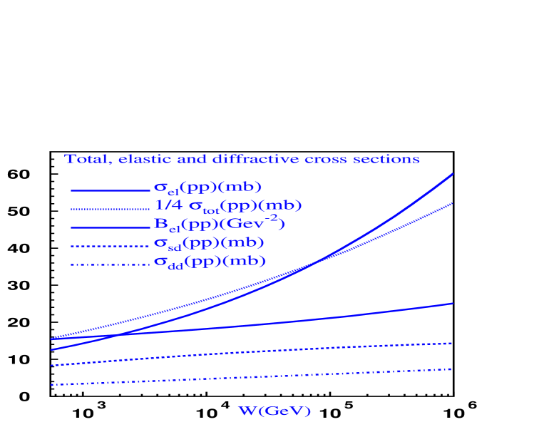
   Figure 5: Total, elastic and diffractive dissociation cross sections in model B(2).

   Model	$\Delta$	$\beta$	$R^{2}_{0;1,1}$	$\alpha^{\prime}_{P}$	$g^{2}_{1,1}$	$g^{2}_{2,2}$	$g^{2}_{\Delta}$	$g^{2}_{1,2}$
   A	0.126	0.464	16.34 $GeV^{-2}$	0.200 $GeV^{-2}$	12.99 $GeV^{-2}$	N/A	145.6 $GeV^{-2}$	N/A
   B(1)	0.150	0.526	20.80 $GeV^{-2}$	0.184 $GeV^{-2}$	4.84 $GeV^{-2}$	4006.9 $GeV^{-2}$	N/A	139.3 $GeV^{-2}$
   B(2)	0.150	0.776	20.83 $GeV^{-2}$	0.173 $GeV^{-2}$	9.22 $GeV^{-2}$	3503.5 $GeV^{-2}$	N/A	6.5 $GeV^{-2}$

   Table 1: Fitted parameters for Models A, B(1) and B(2). $R^{2}_{0;1,2}=R^{2}_{0;\Delta}=0.5R^{2}_{0;1,1}$, $R^{2}_{0;2,2}=0.$

   

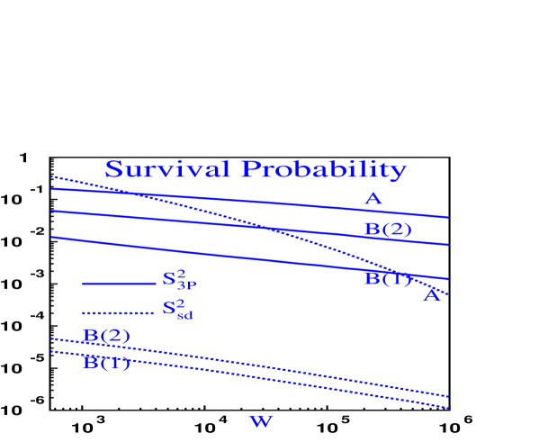
   Figure 6: Survival probabilities for single diffraction $p$-$p$ collision. $S^{2}_{3P}$ (solid line) denotes the survival probability for high mass diffraction dissociation (see Eq. (2.26)). $S^{2}_{sd}$ (dotted line) is the survival probability for diffractive dissociation in the entire kinematic region (see Eq. (2.34). The upper curves (solid and dotted) refer to Model A[16]. The lower curves relate to Model B of Ref.[17].

   We trace this dramatic difference to the relaxation of the constraints on the initial rescatterings. Allowing an additional amplitude, enables increased screening of the input amplitude.

3. An important observation, correlated to the above, is that the unscreened input cross sections of Model B(2) are considerably larger than the unscreened input cross sections of Model A. This is a consequence of the large difference between the fitted values of $g^{2}_{2,2}$ of Model B(2) and $g^{2}_{\Delta}$ of Model A, and, also, the different values of $\Delta$ (the Pomeron intercept) of these models. Since these models provide compatible good reproductions of the fitted data base, we conclude that the large difference in the unscreened cross sections of Models A and B(2) are compensated by the reciprocal difference in the corresponding survival probabilities.

4. The survival probabilities calculated in our two amplitude Model A are in agreement with those calculated by Khoze, Martin and Ryskin in their two channel model[12], which differs from ours. Our present observation that the three amplitude Model B results in considerably smaller $S^{2}$ values, implies that the presumed consistency between most of the published survival probability outputs (for details see Ref.[18]) should be carefully re-examined using more robust models.

5. $S^{2}_{3P}$ are consistently higher than $S^{2}_{sd}$. Note that the input of $\sigma_{sd}(\mbox{high mass})$, described by the triple Pomeron diagram, behaves as $s^{\Delta}$. On the other hand $\sigma_{sd}(\mbox{low mass})$, for which the triple Pomeron diagram is not applicable, behaves as $s^{2\,\Delta}$.

Diffractive processes are very important at cosmic ray energies. Kama et al.[22] have shown that diffractive $p$-$p$ interactions play a crucial role in understanding the spectrum of galactic gamma-rays that come predominantly from $\pi^{0}\rightarrow\gamma\gamma$. The inclusion of diffractive processes makes the gamma ray spectrum harder, and when this is included together with the assumption of Feynman scaling violations, one can explain about half of the ”GeV Excess”. The magnitude of the diffractive cross sections is a crucial element of this and similar studies. A review of our results at cosmic ray energies will be published elsewhere.

3 Survival probability for triple Pomeron vertex in J/$\Psi$-$p$ photo and DIS production

In this section we calculate the survival probabilities for high mass diffraction in the reaction of Eq. (1.4). From Fig. 2 one can see that we need the following ingredients to make these estimates: i) the amplitude for the interaction of a colorless dipole with the target.; and ii) the description of J/$\Psi$ production with no initial state interactions with the target, shown in Fig. 2.

For the scattering dipole amplitude we take a model developed by one of us[19]. This model is based on the solution of a generating functional[23, 24, 25], with an additional assumption that the dipoles do not change their sizes during the interaction. The amplitude is equal to

$$N(Y=\ln(1/x);r,b)\,=\,\frac{\Omega\left(Y;r,b\right)}{1\,+\,\Omega\left(Y;r,b\right)}\,,$$ (3.41)

where

$$\Omega\left(Y;r,b\right)\,=\,\frac{\pi^{2}}{N_{c}}r^{2}\,xG(x_{0},\mu^{2})\;xG\left(\frac{x}{x_{0}},\mu^{2}\,=\,\frac{C}{r^{2}}\,+\,\mu^{2}_{0}\right)\,S(b).$$ (3.42)

$S(b)$ is the proton b-profile,

$$S(b)\,=\,\frac{2}{\pi R^{2}}\frac{\sqrt{8}b}{R}K_{1}\left(\frac{\sqrt{8}b}{R}\right).$$ (3.43)

The saturation scale $Q^{2}_{s}(Y)$ is defined from the condition

$$\Omega\left(Y;r_{s},b\right)\;=\;1\;\;\;\mbox{with}\;\;r^{2}_{s}\;=\;4/Q^{2}_{s}.$$ (3.44)

The gluon structure function $xG(x,\mu^{2})$ satisfies the DGLAP evolution equation with the initial condition $xG(x,Q^{2}_{0})\,=\,A/x^{\omega_{0}}$ at $Q^{2}_{0}\;=\;1\;GeV^{2}$. In other words, Eq. (3.42) describes the contribution of the hard Pomeron that can be calculated in pQCD. All parameters in Eq. (3.42) have been found by fitting to the data on $F_{2}$. The fit is good and has $\chi^{2}/d.o.f.\,=\,1.07$[19]. The values of the fitted parameters, are compatible with the parameter values obtained in other competing models [26]. Eq. (3.43) is the Fourier transform of the electro-magnetic form factor of the proton in t-space. Eq. (3.41) is quite different from the eikonal approximation that has been used in other models, and has a form which is typical for the ‘fan’ diagrams which are summed in the mean field approximation (MFA).

One can see directly from Eq. (3.41) and Eq. (3.42) that

$$N(Y=\ln(1/x);r,b)\,\,\,\,\xrightarrow{r\,\rightarrow\,\infty;\,\;x\,\,fixed}\,\,\,\,1\,,\,\,\,\,\,\,\,\,\,\,\,\,\,N(Y=\ln(1/x);r,b)\,\,\,\,\xrightarrow{x\,\rightarrow\,0;\,\,r\,\,fixed}\,\,\,\,1.$$ (3.45)

In Fig. 7 we show how Eq. (3.41) fits the experimental data.

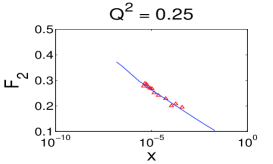
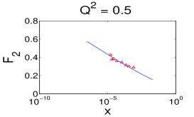
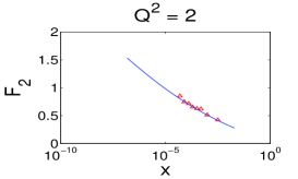
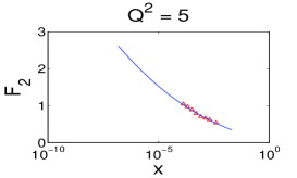
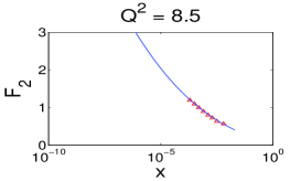
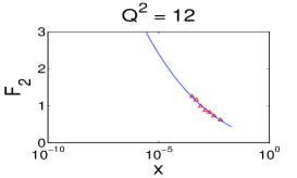
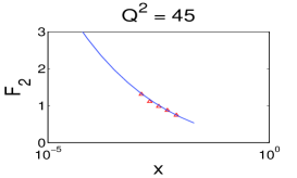
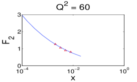
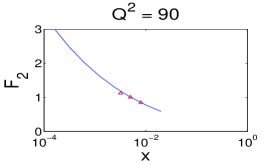
Figure 7: Examples of the fit with Eq. (3.41).

Using Eq. (3.42) we can write the formula for Fig. 2,

$$\sigma\left(\gamma^{*}+p\longrightarrow J/\Psi+M({Fig.~{}\ref{3pjdia}})\right)\,=\,G_{3P}\,(M^{2})^{\Delta_{P}}\,\int\,d^{2}\,b\,\exp\left(-\frac{b^{2}}{R^{2}}\right)\,\times$$ (3.46)

$$\left|\int dz\,d^{2}\,r\,\Psi_{\gamma^{*}}(r,z,Q^{2})A(r,x_{P})\Psi_{J/\Psi}(r,z)\right|\,\times\,\left|\int dz^{\prime}\,d^{2}\,r^{\prime}\Psi_{\gamma^{*}}(r,^{\prime}z^{\prime},Q^{2})A(r^{\prime},x_{P})\Psi_{J/\Psi}(r^{\prime},z^{\prime})\right|,$$

where

$$A\left(r,x_{P};b\right)\,=\,\int\,d^{2}b\,\Omega\left(Y;r,b\right).$$ (3.47)

In Eq. (3.46) we assume that i) that the hard Pomeron in the upper legs of Fig. 2 does not depend on the impact parameter. ii) The triple Pomeron vertex ($HP-P-HP$) coupling is the same as the triple soft Pomeron vertex ($P-P-P$) coupling. $HP$ denotes the hard Pomeron, while $P$ stands for the soft Pomeron. $R$ is the radius of the soft interaction and it was taken to be equal to $R^{2}\,=\,\left(12\,+\,\ln(M^{2}/s_{0})\right)GeV^{-2}$, with $s_{0}=1GeV^{2}$.

The product of the wave functions is taken as[27]

$$\Psi_{J/\Psi}(r,z=\frac{1}{2})\,\times\,\Psi_{\gamma^{*},T}(r;Q^{2})\,=\,\frac{K_{F}}{48\alpha_{em}}\sqrt{\frac{3\Gamma_{ee}M_{\psi}}{\pi}}\,\exp\left(-\,\frac{r^{2}_{\perp}\,m^{2}_{c}}{3\,v^{2}}\right)\,\times$$ (3.48)

$$\hskip 85.35826pt\left\{\frac{a^{2}}{m_{c}}\,\left(\zeta\,K_{1}(\zeta)-\frac{\zeta^{2}}{4}K_{2}(\zeta)\right)+m_{c}\,\left(\frac{\zeta^{2}}{2}\,K_{2}(\zeta)-\zeta\,K_{1}(\zeta)\right)\right\},$$

$$\Psi_{J/\Psi}(r,z=\frac{1}{2})\,\times\,\Psi_{\gamma^{*},L}(r;Q^{2})\,=\,\frac{K_{F}}{48\alpha_{em}}\sqrt{\frac{3\Gamma_{ee}M_{\psi}}{\pi}}\,\exp\left(-\,\frac{r^{2}_{\perp}\,m^{2}_{c}}{3\,v^{2}}\right)\,\times$$

$$\hskip 85.35826pt\left\{\frac{Q}{2}\left(\frac{\zeta^{2}}{2}\,K_{2}(\zeta)-\zeta\,K_{1}(\zeta)\right)\right\}.$$ (3.49)

$\zeta=a\,r$, $K_{i}$ (where i=1,2) are the modified Bessel functions, $\Gamma_{ee}=5.26\,\mbox{KeV}$ is the leptonic width of $J/\Psi$.

$$a^{2}\,=\,z\,(1-z)\,Q^{2}\,+\,m^{2}_{c},\,\,\,\,\,\,\,\mbox{and}\,\,\,\,\,\,\,\,\,\,\,\,x_{P}\,\,=\,\,\frac{Q^{2}\,\,+\,\,M^{2}}{s}.$$ (3.50)

The exponential factor in Eq. (3.48) and Eq. (3.49) which describes the wave function of $J/\Psi$ meson with velocity $v$, has been discussed in Ref.[28] and references therein.

For the diagram of Fig. 2 we can write the expression that takes into account the possible rescatterings before the interaction that produces a $J/\Psi$ meson,

$$\sigma\left(\gamma^{*}+p\longrightarrow J/\Psi+M({Fig.~{}\ref{3pspjdia}})\right)\,\,\,=\,\,\,G_{3P}\,(M^{2})^{\Delta_{P}}\,\,\int\,d^{2}b\,\,\,\exp\left(-\frac{b^{2}}{R^{2}}\right)\,\times$$ (3.51)

$$\left|\int dz\,d^{2}\,r\Psi_{\gamma^{*}}(r,z,Q^{2})\,\,A(r,x_{P})\,\,\left(\,1\,\,\,-\,\,\,N(Y=\ln(1/x);r,b)\,\right)\,\,\Psi_{J/\Psi}(r,z)\right|\,\times\,$$

$$\left|\int dz^{\prime}\,d^{2}\,r^{\prime}\Psi_{\gamma^{*}}(r,^{\prime}z^{\prime},Q^{2})\,\,A(r^{\prime},x_{P})\,\,\left(\,1\,\,\,-\,\,\,N(Y=\ln(1/x);r^{\prime},b)\,\right)\,\,\Psi_{J/\Psi}(r^{\prime},z^{\prime})\right|.$$

The survival probability is the ratio of these two equations (Eq. (3.46) and Eq. (3.51))

$$S^{2}_{3P}(J/\Psi)\,=\,\frac{\sigma\left(\gamma^{*}+p\longrightarrow J/\Psi+M({Fig.~{}\ref{3pspjdia}};\,{Eq.~{}(\ref{SPJ6})})\right)}{\sigma\left(\gamma^{*}+p\longrightarrow J/\Psi+M({Fig.~{}\ref{3pjdia}};\,{Eq.~{}(\ref{SPJ5})})\,\right)}\,.$$ (3.52)

The results of our calculations using Eq. (3.52) are plotted in Fig. 8.

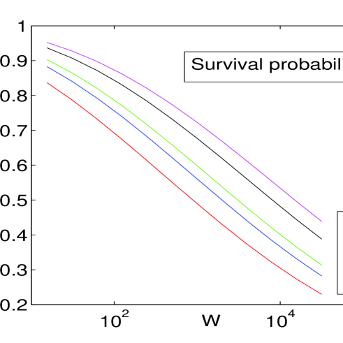
Figure 8: The survival probability for the triple Pomeron vertex in the reaction of Eq. (1.4).

One can see that $S^{2}_{3P}$ is smaller than 1, not compatible with the assumption of Ref.[12]. This should be taken into account when attempting to extract the value of the triple Pomeron vertex from the measurement of the cross section of reaction of Eq. (1.4).

Taking the survival probabilities corrections into account when extracting the value of $G_{3P}$, it is interesting to study the ratio $R\,=\,R_{p}/R_{J/\Psi}$, where

$$R_{p}\,=\,\frac{\sigma\left(p+p\to p+M(M\gg m_{p})\right)}{\sigma\left(p+p\to p+p\right)}\,,$$ (3.53)

$$R_{J/\Psi}\,=\,\frac{\sigma\left(\gamma^{*}+p\to J/\Psi+M(M\gg m_{p})\right)}{G_{3P}\left(\gamma^{*}+p\to J/\Psi+p\right)}\,,$$ (3.54)

so as to validate the theoretical estimates, as well as checking the sensitivity of $G_{3P}$ to the hardness of the coupled Pomerons.

4 Conclusions

In this paper we confirm the wide spread expectation that the survival probability for the triple Pomeron vertex is very small[15, 13, 12]. However, whereas we find the results of our two amplitude Model A almost identical to the results obtained in Ref.[12] (which is also a two amplitude model), our three amplitude model estimates are an order of magnitude smaller. This may also influence the $S^{2}$ calculations for other channels. In particular, it was noted[18] that the various two amplitude calculations of $S^{2}_{CD}$, relevant to exclusive central Higgs production, are in remarkable agreement. This optimistic evaluation should be carefully re-examined.

We stress the importance of $J/\Psi$ SD photoproduction (Eq. (1.4)). Comparing its high mass diffraction data with the corresponding $p$-$p$ scattering, and correcting both channels with their corresponding survival probabilities, we hope to evaluate both the value of $G_{3P}$ and its dependence on the Pomeron’s hardness.

In this context, we emphasize that even though $S^{2}_{3P}$ obtained for Eq. (1.4) is considerably higher than $S^{2}_{3P}$ obtained for $p$-$p$ scattering, its value is less than unity and should not be neglected.

The details of our three amplitude model B, including calculations for hard diffraction, and other LRG configurations will be published in a forthcoming paper.

References

- [1] Yu. L. Dokshitzer, V. Khoze and S.I. Troyan, Proc.“Physics in Collisions 6”, p. 417, ed. M. Derrick, WS 1987; Sov. J. Nucl. Phys. 46, 712 (1987); Yu. L. Dokshitzer, V. Khoze and T. Sjostrand, Phys. Lett. B274, 116 (1992).
- [2] J. D. Bjorken, Int. J. Mod. Phys. A7, 4189 (1992); Phys. Rev. D47, 101 (1993).
- [3] E.A. Kuraev, L.N. Lipatov and V.S. Fadin, Sov. Phys. JETP 45, 199 (1977); Ya.Ya. Balitskii and L.V. Lipatov, Sov. J. Nucl. Phys. 28, 822 (1978); L.N. Lipatov, Sov. Phys. JETP 63, 904 (1986).
- [4] F. Low,Phys. Rev. D12, 163 (1975); S. Nussinov, Phys. Rev. Lett. 34, 1286 (1975); Phys. Rev. D14, 244 (1976).
- [5] E. Gotsman, E.M. Levin and U. Maor, Phys. Lett. B309, 199 (1993).
-
[6]
V.A. Khoze, A.D. Martin, M.G. Ryskin,Phys. Lett. B401,
330 (1997);
Phys. Rev. D56, 5867 (1997);
G. Oderda, G. Sterman, Phys. Rev. Lett. 81, 3591 (1998). - [7] E. Levin, Phys. Rev. D48, 2097 (1993).
- [8] R.S. Fletcher, Phys. Rev. D48, 5162 (1993).
- [9] A. Rostovtsev and M.G. Ryskin, Phys. Lett. B390, 375 (1997) .
- [10] E. Gotsman, E.M. Levin and U. Maor, Nucl. Phys. B493, 354 (1997).
- [11] E. Gotsman, E.M. Levin and U. Maor, Phys. Lett. B438, 229 (1998).
- [12] V.A. Khoze, A.D. Martin and M.G. Ryskin, Phys. Lett. B643 (2006) 93.
- [13] Y.I. Azimov, V.A. Khoze, E.M. Levin and M.G. Ryskin, Sov. J. Nucl Phys. 23, 449 (1976); Nucl. Phys. B89, 508 (1975); V.A. Abramovsky, A.V. Dmitriev and A. A. Schneider, “Diffractive scattering at high energies”, arXiv:hep-ph/0512199; A. Capella, J. Kaplan and J. Tran Thanh Van, Nucl. Phys. B105, 333 (1976); V.A. Abramovsky and R. G. Betman, Sov. J. Nucl. Phys. 49, 747 (1989); K. Goulianos and J. Montanha, Phys. Rev. D59, 114017 (1999); S. Ostapchenko, Phys. Rev. D74, 014026 (2006); Phys. Lett. B636, 40 (2006).
- [14] A.B. Kaidalov, V.A. Khoze, Yu.F. Pirogov and N.L. Ter-Isaakyan, Phys. Lett. B45, 493 (1973).
- [15] A.B. Kaidalov and K.A. Ter-Martirosyan, Nucl Phys B75, 471 (1974); R.D. Field and G.C. Fox, Nucl. Phys. B80, 367 (1974); A.B. Kaidalov, Phys. Rep. 50, 157 (1979).
- [16] E. Gotsman, E. Levin and U. Maor, Phys. Lett. B438, 229 (1998).
- [17] E. Gotsman, E. Levin and U. Maor, Phys. Rev. D60, 094011 (1999).
- [18] E. Gotsman, H. Kowalski, E. Levin, U. Maor and A. Prygarin, Eur. Phys. J. C47, (2006) 655; E. Gotsman, E. Levin, U. Maor, E. Naftali and A. Prygarin, ”HERA and the LHC - A workshop on the implications of HERA for LHC physics: Proceedings Part A”, p. 221 2005, [arXiv:hep-ph/0511060].
- [19] A. Kormilitzin, ”Saturation model in the non-Glauber approach”, [arXiv:hep-ph/07072202].
- [20] E. Gotsman, E. M. Levin and U. Maor, Phys. Rev. D 49 (1994) 4321 [arXiv:hep-ph/9310257].
- [21] T. Affolderr et al., Phys. Rev. Lett. 87, (2001) 141802.
- [22] T. Komae, T. Abe and T. Koe, Astro. J. 620, (2005) 2344.
- [23] A.H. Mueller, Nucl. Phys. B415, 373 (1994); ibid B437, 107 (1995).
- [24] E. Levin and M. Lublinsky, Nucl. Phys. A730, 191 (2004).
- [25] E. Levin and M. Lublinsky, Phys. Lett. B607, 131 (2005).
- [26] K. Golec-Biernat and M. Wusthoff, Eur Phys J. C20, (2001) 313; Phys. Rev., D59, (1999) 014017; Phys Rev. D60, (1999) 114023; H. Kowalski and D. Teaney, Phys Rev. D68, (2003) 114005; J. Bartels, K. Golec-Biernat and H. Kowalski, Phys. Rev. D66, (2002) 014001; K. Golec-Biernat and S. Sapeta, Phys. Rev. D74, (2006) 054032.
- [27] E. Gotsman, E. Levin, M. Lublinsky, U. Maor and E. Naftali, Acta Phys. Polon. B34, 3255 (2003).
- [28] M.G. Ryskin, R.G. Roberts, A.D. Martin and E.M. Levin, Z. Phys. C76, 231 (1997).