IFT-UAM/CSIC-06-06

OUTP-07-01-P

We review the mechanism of radiative electroweak symmetry breaking taking place in SUSY versions of the standard model. We further discuss different proposals for the origin of SUSY-breaking and the corresponding induced SUSY-breaking soft terms. Several proposals for the understanding of the little hierarchy problem are critically discussed.

1 Introduction

The driving force in seeking what lies beyond the Standard Model has been the desire to understand electroweak symmetry breaking and the generation of mass. The Standard Model parameterises this breaking via a stage of spontaneous symmetry breaking generated by a component of the ”Higgs” scalar electroweak doublet field. However it leaves many fundamental questions unanswered. It does not explain what the scale of symmetry breaking should be and provides no underlying reason for the complicated gauge and matter multiplet structure. In addition it requires a large number of parameters to be specified to determine the various interactions needed by the model.

Attempts to explain the structure of the Standard Model usually postulate new physics at a scale above the electroweak scale. The archetypical example of this is Grand Unification or heterotic superstring unification in which the Standard Model gauge group $SU(3)\times SU(2)\times U(1)$ is a subgroup of a simple gauge group such as $SU(5)$, $SO(10)$ or $E_{6},$ broken at a very high scale close to the Planck scale. By unifying the strong, weak and electromagnetic interactions these theories simplify the gauge and multiplet structure and relate many of the parameters of the Standard Model. However Grand Unified models still leave unanswered the fundamental question why the scale of electroweak breaking should be so much less than the Grand Unified scale or the string scale. The problem is particularly acute because radiative corrections to the Higgs sector drive this scale close to the underlying unified scale. To see this consider the potential for the Standard Model Higgs, $h$, given by

$$V={\frac{1}{2}}m^{2}h^{2}+{\frac{1}{4}}\lambda h^{4}\ ,$$ (1)

At one loop order the mass has quadratically-divergent contributions [1]. Treating the Standard Model as an effective field theory valid at scales below $\Lambda_{\mathrm{SM}}$ this contribution is given by

$$\delta_{q}m^{2}={\frac{3}{64\pi^{2}}}(3g^{2}+g^{\prime 2}+8\lambda-8\lambda_{t}^{2})\Lambda_{\mathrm{SM}}^{2}\ ,$$ (2)

where $g,g^{\prime},\lambda$ and $\lambda_{t}$ are the $SU(2)\times U(1)_{Y}$ gauge couplings, the quartic Higgs coupling and the top Yukawa coupling, respectively. The requirement of no fine-tuning between the above contribution and the tree-level value of $m^{2}$ sets an upper bound on $\Lambda_{\mathrm{SM}}$. For a Higgs mass in the range $m_{h}=115-200$ GeV,

$$\left|{\frac{\delta_{q}m^{2}}{m^{2}}}\right|\leq 10\ \Rightarrow\ \Lambda_{\mathrm{SM}}\leqslant 2-3\ \mathrm{TeV}\ .$$ (3)

This is to be compared to the Grand Unified scale or string scale some thirteen or more orders of magnitude higher, which is the expected cutoff in the original unified extensions of the Standard Model! This is the hierarchy problem.  A separation of these scales is possible if the electroweak breaking scale is protected from large radiative corrections by a (spontaneously broken) symmetry. While some limited protection is possible if the Higgs is a pseudo-Goldstone boson (see below) the only symmetry capable of providing protection from a very high scale is supersymmetry (SUSY). This requires that the Standard Model states be accompanied by supersymmetric partners, the squarks and sleptons, the Higgsinos and the gauginos which must get a mass when supersymmetry is broken, the mass scale for these states being limited to be $\leqslant\Lambda_{\mathrm{SM}}$ i.e. roughly within an order of magnitude of the electroweak breaking scale by the need to solve the hierarchy problem.

The breaking of supersymmetry initially seemed to be the stumbling block to implementing the supersymmetric solution to the hierarchy problem because it was known that if supersymmetry breaking is directly coupled to the Standard Model states then the mas of the superpartners obey a sum rule [2] such that a component of each of the squarks and sleptons would be lighter than its quark and lepton partners. Since we have not observed such light scalar states carrying Standard Model quantum numbers this is not a viable possibility. However if supersymmetry should be broken in an ”hidden” sector with no direct couplings to the SM states then the sum rule can be evaded with both components of the squarks and sleptons heavier than their fermion partners. This is because SUSY breaking is only communicated to the visible sector by radiative and/or gravitational corrections involving ”messenger” states and these effects do not obey the sum rule[3],[4],[5]. Initial attempts to explain the magnitude of the hierarchy employed additional symmetries to force the supersymmetry breaking, driven by Yukawa couplings involving messenger states, to be much smaller than the underlying supersymmetry breaking in the hidden sector[6]. Subsequently it was realised that gravitational couplings (SUGRA messengers) present in supergravity theories (theories in which the supersymmetry is made a local symmetry) also provides a coupling between the hidden and visible sectors that makes the supersymmetric scalar partners of the quarks and leptons heavier than their fermion partners [7] . Given the inevitable presence of such supergravity corrections this source of supersymmetry breaking in the hidden sector has enjoyed great popularity. Due to the weakness of gravitational coupling, this “SUGRA” origin for visible sector supersymmetry breaking also is consistent with a high scale of hidden sector scale of supersymmetry breaking, of $O(10^{10}GeV)$.

In constructing phenomenologically viable models of supersymmetry breaking it is essential not to introduce flavour changing neutral current (FCNC) processes at a level much greater than that generated in the Standard Model. This constraint has proved to be extremely restrictive because radiative contributions to flavour changing processes have their supersymmetric analogue in supersymmetric extension of the Standard Model. The simplest way to satisfy the flavour changing constraints is if the squarks and sleptons of the three families are degenerate at the SUSY breaking messenger scale. To achieve this several classes of theories have been constructed in which the coupling between the hidden and visible sectors is due to gravity or to gauge interactions. In the case of gravity, “SUGRA” models, it is not guaranteed that the soft masses are family independent but there are, for example, specific superstring models with this property. For the case of gauge theories, “Gauge Mediated models”, the communication of SUSY breaking from the hidden to the visible sector is by a gauge interaction [8] which is the same for each family. In these schemes the underlying hidden sector scale of supersymmetry breaking can be much smaller (see below).

While supersymmetry offers a solution to the gauge hierarchy problem it introduces new questions. The introduction of scalar partners to the quarks and leptons now means that they, like the Higgs scalar, can acquire vacuum expectation values triggering spontaneous symmetry breaking. This raises the question why should the gauge symmetry group $SU(3)\times SU(2)\times U(1)$ be broken to $SU(3)\times U(1)$ rather than some other subgroup? In theories with Grand Unification or string unification the need to explain why it is the electroweak group that is spontaneously broken becomes even more pressing because each gauge group factor of the Standard Model is on the same footing.

It was in the context of hidden sector SUSY breaking that radiative electroweak breaking was discovered and shown to provide an elegant answer to why it is the electroweak group that is broken and why the breaking scale should be low. Whatever the messenger sector, an initially degenerate spectrum of scalar states at the messenger scale will be non-degenerate at lower scales due to radiative corrections. It is this that naturally leads to radiative electroweak breaking because the radiative corrections can drive the mass squared of a scalar state negative at a scale below the messenger mass scale, triggering spontaneous symmetry breaking at a scale close to the supersymmetry breaking scale in the visible sector. The latter must be low if the hierarchy problem is to be solved. Radiative corrections due to the couplings in the superpotential give a negative contribution to scalar masses squared while those due to gauge couplings give a positive contribution. This means that the direction of spontaneous symmetry breaking is determined by the couplings of the theory. As we shall discuss this provides a natural explanation for the breaking of the Standard Model group to be in the direction $SU(3)\times SU(2)\times U(1)\rightarrow SU(3)\times U(1)_{EM}.$

The price for the supersymmetric solution to the hierarchy problem is that there is a spectrum of supersymmetric states in the visible sector with mass of order the electroweak breaking scale. The fact none has been observed is already somewhat surprising because it reintroduces the need for some fine tuning of parameters to separate the electroweak and supersymmetry breaking scales; this is the “little hierarchy problem”. However there is some circumstantial evidence for the presence of the light supersymmetric partners of the Standard Model states. This comes from the fact that only with their inclusion do the gauge couplings of the Standard Model unify[9],[10] suggesting an underlying stage of unification of the forces. The fact that they unify to a very high degree of accuracy, better than $1\%$[11], is one of the main reasons why supersymmetry is widely considered to be the most likely extension of the Standard model.

In this article we will review the mechanism giving rise to radiative electroweak breaking in supersymmetric theories. In Section 2 we briefly introduce the structure of the minimal supersymmetric extension of the Standard Model (MSSM). Central to the breaking of the Standard Model gauge group are the soft supersymmetry breaking masses and we discuss the various proposals for the soft SUSY breaking terms both in a field theory and a string theory context. In Section 3 we discuss the structure of radiative corrections driving radiative electroweak breaking using the technique of renormalisation group equations and show how it explains the pattern of symmetry breaking observed in the Standard Model. In Section 4 we present a discussion of the ”little hierarchy problem”, comparing the case of supersymmetric solutions to various alternatives that have been suggested. In Section 5 we present a summary and discuss the implications for future experimental searches for the Higgs boson(s) and the supersymmetric partners of Standard Model states.

2 Supersymmetric extension of the Standard Model - the MSSM

The simplest viable supersymmetric extension of the Standard Model involves a single ($N=1$) supersymmetry generator commuting with the Standard Model gauge group so that the symmetry group is the direct product $SU(3)\times SU(2)\times U(1)\times(N=1$ $SUSY).$ The gauge bosons are assigned to vector supermultiplets together with their fermion “gaugino” superpartners. The quarks and leptons are assigned to chiral supermultiplets together with their scalar squark and slepton superpartners. Finally it is necessary to introduce two $SU(2)$ doublets of Higgs scalars (carrying equal but opposite weak hypercharge) making up additional chiral supermultiplets together with their fermion Higgsino superpartners. In the minimal version of the theory the lightest supersymmetric state (the LSP) is stable and is a candidate for dark matter.

2.1 The couplings

The gauge interactions of the states of the theory are now determined. Due to the direct product structure of the gauge symmetry group the new supersymmetric states carry the same gauge quantum numbers as their Standard Model partners and so they have the same couplings to the gauge bosons. Operation by the supersymmetry generator induces new couplings involving the gaugino partner of the gauge bosons and we will not reproduce them here.

The Yukawa couplings and associated quartic scalar couplings come from the superpotential. To reproduce the couplings of the Standard Model requires the following superpotential, $P$

$$P=h_{ijk}L_{i}H_{1j}{E}_{k}\ +\ h{{}^{\prime}}_{ijk}Q_{i}H_{1j}{D}_{k}\ +\ h{{}^{\prime\prime}}_{ijk}Q_{i}H_{2j}{U}_{k}$$ (4)

where $L$ and $E$ ($Q$ and $U,D$ ) are the (left-handed) lepton doublet and antilepton singlet (quark doublet and antiquark singlet) chiral superfields respectively and $H_{1,2}$ are (left-handed) Higgs superfields. The family indices, $i$, $j$ and $k$ are summed over the three families. The supersymmetric couplings correspond to the F terms of the superpotential $P$. These give both Yukawa couplings and pure scalar couplings. For example, the Yukawa couplings following from the first term of eq.(4) are

$$L_{Yukawa}\ =\ h_{ijk}(L_{i}H_{1j}{E}_{k}+{\tilde{L}}_{i}{\tilde{H}}_{1j}E_{k}+L_{i}{\tilde{H}}_{1j}{\tilde{E}}_{k})$$ (5)

where we denote by a supertwiddle the supersymmetric partners to the quarks, leptons and Higgs bosons, namely the squarks, sleptons and Higgsinos. The first term is the usual term in the Standard Model needed to give charged leptons a mass. The new couplings associated with the supersymmetric states related to the first term by the operation of the supersymmetry generator are given by the second and third terms. The scalar couplings associated with eq.4 are

$$L_{scalar}\ =\ \sum_{i,j}\mid{\frac{{\partial^{2}P}}{{\partial\phi_{i}\phi_{j}}}}\mid^{2}$$ (6)

where $\phi_{i}$ are chiral superfields and after differentiation of the superpotential only the scalar components of the remaining chiral superfields are kept. The full set of Feynman rules resulting from the superpotential of eq.4 may be found e.g. in ref. [12].

There is one further coupling needed to complete the couplings of the minimal supersymmetric version of the standard model. In order to generate a mass for the Higgsinos associated with the Higgs doublets $H_{1,2}$ it is necessary to add a term to the superpotential given by

$$P{\ {}^{\prime}}\ =\ \mu H_{1}H_{2}$$ (7)

In addition to giving a mass $\mu$ to the Higgsinos, this term plays an important role in determining the Higgs scalar potential and the pattern of electroweak symmetry breaking. As we will discuss in more detail in section 3 the (SUSY-breaking) scalar term following from eq.(7) aligns the vacuum expectation values (vevs) of the two Higgs fields so that the photon is left massless, obviously a crucial ingredient for a viable theory.

We note that this term is the only one involving a coupling with dimensions of mass. If the theory is to avoid the hierarchy problem $\mu$ must be small, of order the electroweak breaking scale, for the Higgs scalars also get a contribution $\mu^{2}$ to their mass squared. Thus any complete explanation of the electroweak breaking scale must also explain the origin of $\mu$.

2.2 Models of soft SUSY breaking

In order to complete the model it is necessary to specify how supersymmetry is broken. As discussed above the source of supersymmetry breaking has to be in a hidden sector communicated to the visible sector by a messenger sector. Provided the supersymmetry breaking is spontaneous the SUSY breaking terms in the visible sector will be “soft” with dimension less  than or equal to 3 in the Lagrangian. This ensures that the underlying SUSY will still control the hierarchy problem because such soft terms do not affect the ultraviolet behaviour of the theory. The possible terms must respect the gauge symmetry of the Standard Model (SM). The resultant effective low energy field theory Lagrangian below the SUSY breaking scale has the general form

$$L_{g}\ =\ \frac{1}{2}\sum_{a}M_{a}\ \lambda_{a}\lambda_{a}\ +\ h.c.$$ (8)

$$L_{m^{2}}\ =\ -m_{H_{d}}^{2}|H_{d}|^{2}-m_{H_{u}}^{2}|H_{u}|^{2}-m_{Q_{ij}}^{2}Q_{i}Q_{j}^{\ast}-m_{U_{ij}}^{2}U_{i}U_{j}^{\ast}$$

$$-m_{D_{ij}}^{2}D_{i}D_{j}^{\ast}-m_{L_{ij}}^{2}L_{i}L_{j}^{\ast}-m_{E_{ij}}^{2}E_{i}E_{j}^{\ast}$$

$$L_{A,B}\ =\ -\ A_{ij}^{U}Q_{i}U_{j}H_{u}\ -\ A_{ij}^{D}Q_{i}D_{j}H_{d}\ -\ A_{ij}^{L}L_{i}E_{j}H_{d}\ -\ B\ H_{d}H_{u}\ +\ h.c.$$

in standard notation. This has many (107) free parameters beyond the SM. However, as mentioned above, there are strong constraints on the form these terms can take due to the need to avoid large flavour changing processes. For example the SM $\Delta S=2$ amplitude which generates the $K^{0}-\overline{K}^{0}$ mass difference has a box diagram contribution involving two $W-$boson propagators and two fermion propagators involving $u,$ $c$ and $\ t$ quarks. The $GIM$ mechanism forces a cancellation between these contributions and the resultant contribution is dominated by the $u$ and $c$ contributions and is proportional to $(m_{c}^{2}-m_{u}^{2})/M_{W}^{2}.$ To suppress the $\Delta S=2$ contribution below the experimental limit requires $(m_{c}^{2}-m_{u}^{2})/M_{W}^{2}\leqslant 10^{-4}$ which is satisfied for a charm quark mass of $O(1GeV)$ as observed.

The analogous contribution from the Standard Model supersymmetric partners involves two “Wino”, $\widetilde{W},$ fermion propagators, the partners of the $W-$bosons, and two scalar propagators involving the $\widetilde{u},$ $\widetilde{c}$ and $\ \widetilde{t}$ squarks, the scalar partners of the $u,$ $c$ and $\ t$ quarks . For Winos heavier than squarks this contribution is proportional to $(m_{\widetilde{c}}^{2}-m_{\widetilde{u}}^{2})/M_{\widetilde{W}}^{2}.$ To suppress the new SUSY contribution below the experimental limit requires[13] $(m_{\widetilde{c}}^{2}-m_{\widetilde{u}}^{2})/M_{\widetilde{W}}^{2}\leqslant 10^{-4}.$ For Wino masses less than $1TeV,$ as is required by the SUSY solution to the hierarchy problem,  implies $m_{\widetilde{c}}^{2}-m_{\widetilde{u}}^{2}\lesssim\ 10GeV^{2}$ a surprising result given that the non-observation of squarks requires that they are much heavier than the W-boson. This near-degeneracy for the squarks of the first two families is made even more stringent because, unlike the gluon contribution in the Standard Model, the gluino contribution in its supersymmetric extension also changes strangeness and contributes to the box diagram, giving a contribution enhanced by the strong coupling involved. Given this fact, viable methods of supersymmetry breaking must explain why the squarks are nearly degenerate.

In specific scenarios of SUSY-breaking many or all the couplings are diagonal in family space and there are also unification constraints so that the number of parameters is drastically reduced. This depends on the origin of SUSY-breaking is. Here we will briefly review the most popular ideas for the mediation of SUSY-breaking.

Supergravity mediation[7]

This is a well motivated option, since gravity is there anyhow and combined with SUSY gives rise to supergravity. Asuming there is some hidden SUSY-breaking sector in the theory, the spin=3/2 partner of the graviton, the gravitino, gets a mass $m_{3/2}$ of order $<F>/M_{P}$, $<F>\not=0$ being some SUSY-breaking scalar auxiliary field. One of the generic features of supergravity is that gauge couplings as well as kinetic terms are field dependent. The Lagrangian is defined by three classes of functions: the gauge kinetic functions $f_{a}(\phi_{i})$ (one per group), the Kahler potential $K(\phi,\phi^{\ast})$ and the superpotential $W$. Soft terms may be explicitly evaluated in terms of those functions, the gravitino mass, and the values of the auxiliary fields $F$ breaking SUSY. For example, if the Kahler metrics of the SM scalar fields are diagonal one can write

$${M_{a}} =\frac{1}{2\mathrm{Re\,}{\ f_{a}}}{F^{M}}\partial_{M}{f_{a}}\ ,$$

$${m_{I}^{2}} ={m_{3/2}^{2}}-\sum_{M,N}{\bar{F}^{\bar{M}}F^{N}}\partial_{\bar{M}}\partial_{N}\log({\tilde{K}_{I\bar{I}}})\ ,$$ (9)

$${A_{IJL}} ={F^{M}}[{\ K_{M}}+\partial_{M}\log(Y_{IJL})-\partial_{M}\log({\tilde{K}_{I\bar{I}}\tilde{K}_{J\bar{J}}\tilde{K}_{L\bar{L}})}]\ .$$

where ${\tilde{K}_{II}}$ are the kinetic terms of the SM matter fields. If the vevs of the auxilary fields are of order $<F^{N}>\propto(10^{11}GeV)^{2}$ then the gravitino mass and the soft terms will be of order the electroweak scale, $O(10^{2}GeV)$. The simplest scheme of this type is that of the minimal supergravity model (mSUGRA) which assumes universality of gauge kinetic functions $f_{a}=f$, minimal matter kinetic terms ${\tilde{K}}_{II}=\delta_{II}$ and constant Yukawa couplings. Under these circumstances the scalar masses are family independent as required by FCNC and there are only 4 SUSY-breaking parameters, $M,$ the common gaugino mass, $m$, the common scalar mass, $A$, the common coefficient of the soft trilinear terms and $B$ the coefficient of the soft bilinear term. This scenario is atractive because of its simplicity and has been very much analyzed in the last twenty years. In spite of increasing experimental constraints, the mSUGRA secenario is consistent with radiative EW symmetry breaking and for reduced regions of parameter space can accomodate the appropriate amount of dark matter in the form of the relic SUSY LSP(see ref. [14, 15, 16, 17, 18] for recent analyses). As we will discuss below, specific gravity mediation scenarios naturally appear also in the context of string theory, in which the functions $f_{a},{\tilde{K}},K$ and $W$ may be computed in simple compactifications.

Gauge mediation[8, 19]

In this scheme the leading mediators of SUSY-breaking are the SM gauge bosons and their gaugino partners. In the simplest ‘minimal’ GMSB model [19] one has a singlet chiral super field $X$ with $<X>\not=0$ and $<F_{X}>\not=0$, breaking SUSY. It couples to new, heavy, vector-like fields with SM quantum numbers which make up complete $SU(5)$ representations (e.g., $(5+{\bar{5}})$). Then SM gaugino masses appear at one loop and scalar masses at two loops yielding e.g.

$${M_{a}}\ \simeq\ \frac{{\alpha_{a}}}{4\pi}\left(\frac{{F_{X}}}{<{X}>}\right)\ ;\ {m_{\tilde{q}}^{2}}\ \simeq\ \left(\frac{{F_{X}}}{<{X}>}\right)^{2}\sum_{a}\left(C_{a}(\frac{{\alpha_{a}}}{4\pi})^{2}\right)$$ (10)

with $C_{a}$ the quadratic Casimirs of SM groups. This means that in order to get soft terms of order $M_{W}$ one should have $F_{X}/<X>\simeq 100$ TeV. In this case the LSP is the gravitino ($m_{3/2}\simeq 10-100$ eV) and typically the next-to-LSP(NLSP) is a neutralino or a charged slepton. The typical experimental signatures for this scheme are processes with missing energy plus a photon or lepton (the NLSP may decay inside the detector). One serious problem of the simplest GMSB scenarios is the difficulty in getting an appropriately large B and/or $\mu$ parameters. On the other hand its great virtue is that FCNC are very small, since gauge transmission is flavor-blind and renormalization effects are small.

Anomaly mediation[20]

This mechanism is a variety of gravity mediation. It was observed that in the presence of SUSY-breaking in supergravity, there is always a class of one-loop soft terms appearing for all SM particles, even if for some reason all Planck mass supressed couplings of hidden sector fields to the SM were absent. They are due to a conformal anomaly which arises because potentially logarithmically divergent radiative corrections depend on a mass scale which breaks conformal invariance. The atractive aspect of anomaly mediation is that its effect is determined by the one-loop terms of the low-energy effective theory, independent of ultraviolet physics, i.e.they only depend on the $\beta$-functions and anomalous dimensions $\gamma_{f}$ of the SSM fields. In particular one has

$${M_{a}}\ =\ \frac{{\beta_{a}}}{{g_{a}}}{m_{3/2}}$$ (11)

$${m_{f}^{2}}\ =\ -\frac{1}{4}\left(\frac{\partial{\gamma_{f}}}{\partial{g}}{\beta_{g}}+\frac{\partial{\gamma_{f}}}{\partial{Y}}{\beta_{Y}}\right){m_{3/2}^{2}}$$ (12)

$${A_{Y}}\ =\ -\frac{{\beta_{Y}}}{{Y}}{m_{3/2}}$$ (13)

wher $Y$ denote the corresponding Yukawa coupling. Note that soft terms are of order $(\alpha/4\pi)m_{3/2}$ and gaugino masses are not universal but rather are on the ratios $M_{1}:M_{2}:M_{3}=2.8:1:7.1$. This implies that typically the LSP is the neutral wino and there is a relatively light chargino. As we said the nicest feature of anomaly mediation is its independence of the UV physics. It also leads to degenerate squarks masses, suppressing unwanted FCNC. On the other hand, although this contribution is always present, it is difficult to construct explicit supergravity/string scenarios in which they are the leading effect (see however comments at the end of the next section). Furthermore one finds from above formulae that the sleptons have negative mass², which makes the simplest anomaly mediation models not viable. On the other hand simple extensions including e.g. the contribution of D-terms from an extra $U(1)$ symmetry[21] or contributions from string moduli[22] can cure this desease.

2.3 String Theory and SUSY-breaking

We have mentioned above several different possibilities considered in the literature for the understanding of the origin and/or structure of SUSY breaking in SUSY versions of the SM. Whatever the solution proposed, one would like to embed the SUSY-breaking inside an ultraviolet consistent theory which also incorporates gravity. The only candidate known to date for a consistent unification of quantum gravity and the SM is string theory. One SUSY breaking mechanism which appears very naturally in the context of string theory is gravity mediation. Indeed, generic string compactifications with SM-like massless quark/lepton spectrum have additional massless singlet chiral fields, the moduli, whose couplings to ordinary matter are Planck-mass suppressed. These include the complex dilaton $S$ (whose real part is related in some compactifications to the inverse gauge coupling constant), the Kahler moduli $T_{i}$ (whose real parts describe the size of the compact 6 extra dimensions) and the complex structure $U_{j}$ (which describe the shape of the extra dimensions). These singlet fields are natural candidates to constitute the hidden sector responsible for SUSY-breaking. Thus the idea is that it is the non-vanishing of the auxiliary fields $F_{S}$,$F_{T_{i}}$, $F_{U_{i}}$ which would be the seed of SUSY breaking. As we will emphasize below, it has been recently realized that non-vanishing values for certain 10-dimensional bosonic fields (Ramond-Ramond and NS-NS backgrounds) do indeed give rise to non-vanishing expectation values to the auxiliary fields of the moduli. Such terms in turn generate SUSY-breaking soft terms for the SM fields. Another ingredient which naturally appears in the context of string theory is the generic presence of extra hidden sector gauge groups which may trigger SUSY-breaking (inducing vevs for the auxiliary fields mentioned above) upon gaugino condensation [23].

In order to compute SUSY-breaking soft terms within this scheme, we need to know the dependence of the gauge kinetic functions $f_{a}$ , the Kahler metrics ${\tilde{K}}_{IJ}(S,T_{i},U_{j})$ of the SM chiral superfields and the Kahler potential of the moduli $K(S,T_{i},U_{j})$. All these quantities may be computed to leading order for some simple compactifications. Then gaugino masses, scalar masses and trilinear A-terms may be computed from the general expressions in eq.(9). The dependence of $f_{a}$, ${\tilde{K}}_{IJ}(S,T_{i},U_{j})$ and $K(S,T_{i},U_{j})$ on the moduli depend on the specific way in which the SM is embedded into string theory. In particular they depend on whether we are dealing with heterotic or e.g. Type IIA or Type IIB orientifold D-brane models. This is not the place to give a detail review of these issues but let us give some example of the kind of relationships among soft terms that one can encounter in some simple compactification scenarios:

• Dilaton domination boundary conditions. If the origin of SUSY breaking in an heterotic string model is the auxiliary field of the dilaton one finds the relationship among SUSY-breaking soft terms [24, 25]:

  $$M\ =\ \sqrt{3}m\ =\ -A$$ (14)

  These boundary conditions are flavour independent, which is welcome in order to avoid large FCNC effects. It turns out that such type of boundary conditions do appear in other string constructions. For example, if the SM is embedded inside (anti-)D3-branes in Type IIB orbifolds and/or orientifolds [26]. In this case the origin of the non-vanishing auxiliary field for the dilaton may be understood in terms of RR-NS flux backgrounds. These boundary conditions are simple and very constraining. In fact if one takes at face value these boundary conditions and does the renormalisation group running from a GUT scale of order $10^{16}$ GeV down to low energies one finds that charge- and color-breaking minima appear [27]. On the other hand, as emphasized in [28] some string models with an intermediate string scale $M_{string}\propto 10^{10}$ GeV such charge/color-breaking minima disappear.

• Heterotic-like T-modulus dominance.

  In heterotic compactifications if the auxiliary field of the volume modulus $T$ is the only non-vanishing, one gets the standard no-scale structure [29]. This means in fact that to leading order all soft terms vanish $M=m=A=0$. However both loop corrections and world-sheet instanton corrections induce non-vanishing soft terms (see e.g.[25]). However those are model dependent and no sharp model-independent prediction can be made.

• Type IIB orientifold T-modulus dominance. It turns out that T-modulus dominance has a different effect on different types of string theory vacua. In particular, in the case of Type IIB orientifolds with the SM gauge group residing on D7-branes, if the SM fields are assumed to behave like the scalars which parametrize the position of D7-branes in extra dimensions, one obtains the simple boundary conditions [30]

  $$m\ =\ M\ ;\ A\ =\ -3M\ ;\ B\ =\ 2M\mu$$ (15)

  This scheme, called ‘fluxed MSSM’ in ref.[30] is very restrictive since it also gives a prediction for the elusive $B$-parameter and has no SUSY CP-problem. In ref.[31] it was shown that these relationships are consistent with correct radiative electroweak symmetry breaking and other phenomenological constraints. If one insists in obtaining the appropriate neutralino dark matter abundance a quite heavy spectrum of sparticles is predicted [31].

• Modulus dominance in a specific MSSM-like IIB orientifold. One can construct concrete Type IIB orientifold models with overlapping ‘magnetized’ D7-branes with a massless spectrum very close to that of the MSSM [32]. These are models based on Type IIB string theory compactified on a $Z_{2}\times Z_{2}$ orientifold with D7-branes. In this settings one can compute the relevant $f_{a}$, ${\tilde{K}}_{IJ}(S,T_{i},U_{j})$ and $K(S,T_{i},U_{j})$ to leading order [34, 33]. Assuming that the auxiliary field of the overall modulus T dominates one finds in a certain approximate limit soft terms of the form [35]

  $$m^{2}\ =\ \frac{M^{2}}{2}\ ;\ A\ =\ -\frac{3}{2}M\$$ (16)

  Again in these examples one can understand the non-vanishing value of the modulus auxiliary field $F_{T}$ as originating on the presence of certain RR and NS 10-dimensional field fluxes. A study of the phenomenological consequences of analogous models has been presented in [36].

These examples do not exhaust at all the possibilities but they show that, at least in certain simplified string model compactifications, one can obtain specific predictions for the structure of soft terms. Other schemes have been considered recently in the context of variants of the KKLT scenario [37] for moduli fixing in string theory. In particular in refs.[38] it has been shown that in certain KKLT-like scenarios of moduli fixing with large-volume Calabi-Yau flux compactifications of Type IIB string theory, one recovers in certain approximation the dilaton dominated kind of boundary conditions described above. In other KKLT-inspired schemes it has been argued that a mixture of anomaly and modulus mediation arises [39]. Recent progress has also been achieved in obtaining string models with gauge mediated SUSY-breaking [40]. In any event it is clear that, if SUSY is found at LHC, measuring the SUSY spectrum and couplings would give important information about the structure of the underlying string theory.

3 Radiative Electroweak Symmetry Breaking

Once one has an understanding of the soft SUSY breaking parameters it is possible to address the question whether there is a stage of spontaneous symmetry breaking by studying the scalar potential. As we have seen in the supersymmetric extension of the Standard Model there are a large number of scalar fields and many possible direction of spontaneous symmetry breaking corresponding to the various possible combinations of these scalar fields that can acquire vacuum expectation values (vevs). To simplify the discussion we first discuss the potential involving only the Higgs scalar fields and later return to a discussion why these are the only fields that acquire vevs, explaining why the breaking is in the direction $SU(3)\times SU(2)\times U(1)$ $\rightarrow SU(3)\times U(1).$

From the gauge interactions and the interactions following from the superpotential of eq(4) the Higgs scalar potential has the form

$$V(H_{1},H_{2})\ =\ {\frac{{{g_{2}}^{2}}}{2}}\ (H_{1}^{\ast}{\frac{{\tau^{a}}}{2}}H_{1}+H_{2}^{\ast}{\frac{{\tau^{a}}}{2}}H_{2})^{2}\ +\ {\frac{{{g_{1}}^{2}}}{8}}\ (|H_{1}|^{2}-|H_{1}|^{2})^{2}\$$

$$+\ {\mu_{1}}^{2}\ |H_{1}|^{2}\ +\ {\mu_{2}}^{2}\ |H_{2}|^{2}\ -\ {\mu_{3}}^{2}(H_{1}H_{2}\ +h.c.\ )$$ (17)

where $\tau^{a},a=1,2,3$ are the $SU(2)_{L}$ Pauli matrices and

$${\mu_{1}}^{2}\ \equiv m_{0}^{2}\ +\ \mu_{0}^{2}\ ;\ {\mu_{2}}^{2}\ \equiv\ m_{0}^{2}\ +\ \mu_{0}^{2}\ ;\ {\mu_{3}}^{2}\ \equiv\ B_{0}\mu_{0}\ .$$ (18)

This is the SUSY version of the ‘Mexican hat’ Higgs potential of the standard model. However, this potential as it stands looks problematic. Indeed, in order to get a non-trivial minimum we need to have a negative $mass^{2}$ eigenvalue in the Higgs mass matrix, i.e., we need $\mu_{1}^{2}\mu_{2}^{2}-\mu_{3}^{4}\ <0$. However, since $\mu_{1}^{2}=\mu_{2}^{2}>0$, this may only happen if $\mu_{1}^{4}=\mu_{2}^{4}<\mu_{3}^{4}$ in which case the scalar potential is unbounded below in the direction $<H_{1}>=<H_{2}>\rightarrow\infty$. The puzzle is resolved [3],[4],[5],[41]  by noting that the boundary conditions eq.18 apply only at the unification or Planck scale. At any scale below one has to consider the quantum corrections to the scalar potential which can be substantial. Consider for example the one-loop corrections to the masses of the Higgs fields. These come from graphs which involve the Yukawa couplings of the Higgs field $H_{2}$ to the u-type quarks and squarks. Of course, these corrections will be negligible except for the ones involving the top quark which has a relatively large Yukawa coupling (for simplicity we ignore here the possibility of a large bottom Yukawa coupling).

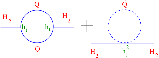
Figure 1: One loop contributions to the Higgs mass in the MSSM.

While supersymmetry is a good symmetry the first graph in fig. 1 leads to a (negative) quadratically divergent contribution which is exactly cancelled by the second graph. Once susy is broken the sparticles get masses and the right-hand diagram is suppressed compared to the left-hand one leaving an overall uncanceled $negative$ contribution [3],[4],[5],[41]

$$\delta\mu_{2}^{2}\ \simeq\ -{\frac{3}{{16\pi^{2}}}}h_{t}^{2}m_{\tilde{Q}}^{2}\log(M_{X}^{2}/(\mu^{2}+m_{\tilde{Q}}^{2}))\ .$$ (19)

where the contribution is evaluated at a scale $\mu.$ If $h_{t}$ is large enough (i.e., if the top quark is heavy enough) this negative contribution may, at a scale below M${}_{X},$ overwhelm the original positive contribution and trigger electroweak symmetry breaking. Similar diagrams exist for the other Higgs field $H_{1}$ but those are expected to give small contributions since they will be proportional to the bottom Yukawa coupling.

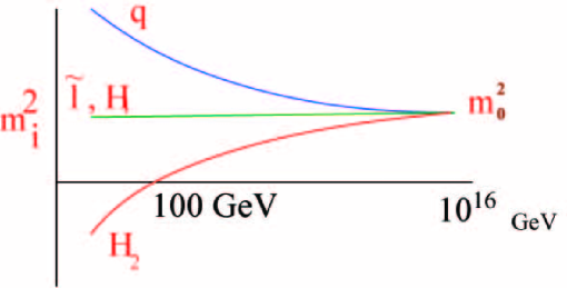
Figure 2: Loop effects trigger the electroweak symmetry breaking in a natural way. The mass² of the Higgs scalars gets negative as the energy decreases, meanwhile squark/slepton mass² remain positive.

One may worry that one can find similar graphs involving squarks such as ${\tilde{t}},{\tilde{b}}$ that could drive their $mass^{2}$ negative leading to minima with broken charge and colour. Indeed these graphs exist but coloured scalars also get large ( positive) contributions to their $mass^{2}$ from loops involving gluinos which are proportional to the large strong coupling constant, preventing $SU(3)\otimes U(1)_{em}$ breaking. The resulting pattern of running masses for the Higgs scalar and the various sparticles of the MSSM is shown in Figure 2. From this one sees that the structure of the minimal supersymmetric standard model is such that quantum corrections select the desired pattern of $SU(3)\otimes SU(2)\otimes U(1)$ symmetry breaking in a natural and elegant way. Note that the proposal for radiative electroweak breaking relied on a heavy top quark anticipating the subsequent measurement of the top quark mass, $m_{t}=$ $O(170GeV)!$

With $\mu_{2}^{2}\not=\mu_{1}^{2}$ the potential in eq.(17) is perfectly well behaved and one can see it is minimized for [4, 42]

$$\nu^{2}\ \equiv\ \nu_{1}^{2}+\nu_{2}^{2}\ =\ {\frac{{2(\mu_{1}^{2}-\mu_{2}^{2}-(\mu_{1}^{2}+\mu_{2}^{2})cos2{\beta})}}{{(g_{2}^{2}+g_{1}^{2})cos2\beta}}}$$ (20)

where $\nu_{1,2}=<H_{1,2}^{0}>$ and $sin2\beta\equiv 2\mu_{3}^{2}/(\mu_{1}^{2}+\mu_{2}^{2})$. The existence of a non-vanishing $\mu_{3}^{2}$ forces the two vevs to be aligned in such a way that electric charge remains unbroken. The W mass is related to $\nu$ via $\nu^{2}=2M_{W}^{2}/g^{2}$. This condition may be equivalently written [43]

$${\frac{{\nu_{2}^{2}}}{{\nu_{1}^{2}}}}\ =\ {\frac{{\mu_{1}^{2}+{\frac{1}{2}}M_{Z}^{2}}}{{\mu_{2}^{2}+{\frac{1}{2}}M_{Z}^{2}}}}\$$ (21)

where $\mu_{1,2}^{2}$ should be evaluated at the weak scale. Thus in a model with the correct $SU(2)\times U(1)$ breaking the parameters are constrained in such a way that $\mu_{1,2}^{2}(M_{W})$ and $\mu_{3}^{2}(M_{W})$ satisfy the above conditions. As we discussed in Section 2 the free parameters in the minimal supergravity model are just

$$m_{0}\ ,\ m_{1/2}\ ,\ A_{0}\ ,\ \mu_{03}^{2}\equiv B_{0}\mu_{0}\ ,\ \mu_{0}$$ (22)

plus the Yukawa couplings, of which $h_{t}$ is likely to be the only one playing an important role in the running of the soft terms. In order to see how all these parameters are constrained we need to use the renormalisation group equations which relate the values of couplings and masses at the unification scale with their values at the weak scale. The renormalisation group equations generalise the analysis of radiative corrections given in eq.19 allowing for the summation of all powers of the logarithmic corrections.

3.1 Renormalisation Group analysis

The renormalisation group equations for the Yukawa couplings [42] can be integrated analytically in the case in which one only keeps the top-quark Yukawa coupling. For the third generation one finds [43]

$$h_{t}^{2}(t)\ =\ h_{t}^{2}(0)\ {\frac{{E_{1}(t)}}{{1+6Y_{t}(0)F_{1}(t)}}}$$ (23)

$$h_{b}^{2}(t)\ =\ h_{b}^{2}(0)\ {\frac{{E_{2}(t)}}{{(1+6Y_{t}(0)F_{1}(t))^{1/6}}}}$$ (24)

$$h_{\tau}^{2}(t)\ =\ h_{\tau}^{2}(0)\ E_{3}(t)\ ,$$ (25)

where $t\equiv 2\log(M_{X}/Q)$ and $E_{1,2,3}$ and $F_{1}$ are known functions of $\alpha_{i}(t)$ and $Q$ is the scale at which the couplings are evaluated. The $E_{i}$ functions give just the usual gauge anomalous dimension enhancement whereas the effect of the top Yukawa coupling in the running gives the extra factor. Let us first discuss the case of the top quark. Notice that for small $h_{t}(0)$ one recovers the well-known gauge anomalous dimension result. However, for $Y_{t}(0)\rightarrow\infty$ one gets

$$h_{t}^{2}(t)\ =\ {\frac{{(4\pi)^{2}E_{1}(t)}}{{6F_{1}(t)}}}$$ (26)

independently of the original value of $Y_{t}(0)$, i.e., there is an infrared fixed point. At the weak scale ($t\simeq 67$) one obtains $E_{1}\simeq 13$ and $F_{1}\simeq 290$ which gives an upper bound for the top-quark mass

$$m_{t}\ =\ h_{t}\nu_{2}\ \leq\ h_{t}\nu\ \leq\ 190\ GeV\ .$$ (27)

Let us now consider the running of the mass parameters which are the ones of direct relevance to the $SU(2)\times U(1)$-breaking process. In particular, consider the running of the squarks, sleptons and Higgs masses. The renormalisation group equations describing the mass² evolution have a gauge contribution proportional to gaugino masses and a second contribution proportional to the top-Yukawa coupling². The gauge piece makes the mass² increase as the energy decreases. In particular, squarks get more and more massive as we go to low energies since their equation is proportional to $\alpha_{3}$. The piece in the equations proportional to the top Yukawa coupling has the opposite effect and decreases the mass² as the scale decreases. This effect is normally not big enough to overwhelm the large positive contribution to the mass² of squarks involving the QCD coupling but may be sufficiently large to overwhelm the positive contribution of weakly interacting scalars which only involve the electroweak couplings. The only such scalar in which this can happen is $H_{2}$ since it is the only one (unlike sleptons) which couples directly to the top Yukawa. This is nothing but the renormalisation group improved version of the mechanism in eq.19 . We thus see that the quantum structure of the MSSM leads automatically to the desired pattern of symmetry breaking in a natural way. The qualitative behaviour of the running of scalars is shown in fig. 2.

Apart of obtaining the desired pattern of symmetry breaking one is interested in finding out the spectrum of sparticles in this scheme. Since there are only a few free parameters one has strong predictive power. In the case of the squarks and sleptons, integration of the renormalisation group equations (neglecting Yukawa couplings) leads to the following result [43],[12]

$$m_{{\tilde{U}}_{L}}^{2}\ =\ m_{0}^{2}+2m_{1/2}^{2}({\frac{4}{3}}{\tilde{\alpha}}_{3}f_{3}+{\frac{3}{4}}{\tilde{\alpha}}_{2}f_{2}+{\frac{1}{{36}}}{\tilde{\alpha}}_{1}f_{1})+cos(2\beta)M_{Z}^{2}({\frac{{-1}}{2}}+{\frac{2}{3}}sin^{2}\theta_{W})$$ (28)

$$m_{{\tilde{D}}_{L}}^{2}\ =\ m_{0}^{2}+2m_{1/2}^{2}({\frac{4}{3}}{\tilde{\alpha}}_{3}f_{3}+{\frac{3}{4}}{\tilde{\alpha}}_{2}f_{2}+{\frac{1}{{36}}}{\tilde{\alpha}}_{1}f_{1})+cos(2\beta)M_{Z}^{2}({\frac{1}{2}}-{\frac{1}{3}}sin^{2}\theta_{W})$$

$$m_{{\tilde{U}}_{R}}^{2}\ =\ m_{0}^{2}+2m_{1/2}^{2}({\frac{4}{3}}{\tilde{\alpha}}_{3}f_{3}+{\frac{4}{9}}{\tilde{\alpha}}_{1}f_{1})-cos(2\beta)M_{Z}^{2}({\frac{2}{3}}sin^{2}\theta_{W})$$

$$m_{{\tilde{D}}_{R}}^{2}\ =\ m_{0}^{2}+2m_{1/2}^{2}({\frac{4}{3}}{\tilde{\alpha}}_{3}f_{3}+{\frac{1}{9}}{\tilde{\alpha}}_{1})+cos(2\beta)M_{Z}^{2}({\frac{1}{3}}sin^{2}\theta_{W})$$

$$m_{{\tilde{E}}_{L}}^{2}\ =\ m_{0}^{2}+2m_{1/2}^{2}({\frac{3}{4}}{\tilde{\alpha}}_{2}f_{2}+{\frac{1}{4}}{\tilde{\alpha}}_{1}f_{1})+cos(2\beta)M_{Z}^{2}({\frac{1}{2}}-sin^{2}\theta_{W})$$

$$m_{{\tilde{\nu}}_{L}}^{2}\ =\ m_{0}^{2}+2m_{1/2}^{2}({\frac{3}{4}}{\tilde{\alpha}}_{2}f_{2}+{\frac{1}{4}}{\tilde{\alpha}}_{1}f_{1})-cos(2\beta){\frac{1}{2}}M_{Z}^{2}$$

$$m_{{\tilde{E}}_{R}}^{2}\ =\ m_{0}^{2}+2m_{1/2}^{2}({\tilde{\alpha}}_{1}f_{1})+cos(2\beta)M_{Z}^{2}sin^{2}\theta_{W}$$

where $\theta_{W}$ is the weak angle, $M_{Z}$ is the $Z^{0}$ mass and $m_{0},m_{1/2}$ and $tg\beta=\nu_{2}/\nu_{1}$ are related to the free parameters in eq.22. In this equation

$${\tilde{\alpha}}_{i}\ \equiv\ {\frac{{\alpha_{i}(M_{X})}}{{(4\pi)}}}\ ;\ f_{i}\ \equiv\ {\frac{{(2+b_{i}{\tilde{\alpha}}_{i}t)}}{{(1+b_{i}{\tilde{\alpha}}_{i}t)^{2}}}}t$$ (29)

where $b_{i}=(-3,1,11)$ are the one-loop coefficients of the $\beta$-function of the $SU(3)\otimes SU(2)\otimes U(1)$ interactions. The above equations assume universal soft masses $m_{0}$ for all the scalars in the theory at the unification scale as well as universal gaugino masses $m_{1/2}$. The right-most term in eqs.3.1 does not in fact come from the integration of the r.g.e.’s but from the contribution of the D²-term in the scalar potential of sfermions once $SU(2)\times U(1)$ is broken. As noted above the squarks will be heavier than the sleptons since $\alpha_{3}\gg\alpha_{2}$.

4 The Little Hierarchy Problem

Low energy supersymmetry was introduced to solve the hierarchy problem. To quantify how well it has achieved this we need to modify eq(2) to include the contributions of the new SUSY states as in eq(19). Solving for the minimum of the Higgs scalar potential one finds a bound on the Higgs mass of the form [44]

$$m_{h}^{2}\leq M_{Z}^{2}\cos^{2}2\beta+{\frac{3m_{t}^{4}}{2\pi^{2}v^{2}}}\log{\frac{M_{\widetilde{\mathrm{t}}}^{2}}{m_{t}^{2}}}+...$$ (30)

where $M_{\widetilde{\mathrm{t}}}^{2}$ is an average of stop masses squared. The first term is the tree level contribution to the Higgs mass, small because in SUSY the quartic Higgs coupling, c.f. eq(1) is given by $\lambda=(1/8)(g^{2}+g^{\prime 2})\cos^{2}2\beta$ . The radiative corrections are necessary to increase $m_{h}$ beyond the experimental bound, $m_{h}\geq 115$ GeV. In order to satisfy this mass bound one is forced to live in a region of relatively large soft masses, $M_{\widetilde{\mathrm{t}}}\geq 300$ GeV.

This leads to a conflict with the hierarchy problem because the mass is so large that it requires some fine tuning to keep the electroweak breaking scale low. To see this note that the electroweak breaking scale, which is characterised by $M_{Z},$ depends on the input parameters of the theory. The input parameters are defined at the SUSY breaking messenger scale, $M_{mess},$ and the RG running can introduce large logs if the scale is large which in turn drive the electroweak breaking scale large. The $Z$ mass immediately follows from eq(20) and the main contribution to the negative Higgs mass squared parameter triggering electroweak breaking coming from loops of tops and stops is approximately given by

$$-\frac{3h_{t}^{2}}{4\pi^{2}}(M_{\widetilde{\mathrm{t}}}^{2}+|A_{t}|^{2})\ln\left(\frac{M_{mess}}{M_{\widetilde{\mathrm{t}}}}\right).$$

Putting all this together in the case of the MSSM with gravity mediation, $M_{mess}=M_{Planck},$ one finds for $\tan\beta=2.5$[45]

$$\frac{M_{Z}^{2}}{2} =-.87\,\mu^{2}(0)+3.6\,{M_{3}^{2}(0)}-.12\,{M_{2}^{2}(0)}+.007\,{M_{1}^{2}(0)}$$

$$-.71\,{m_{H_{U}}^{2}(0)}+.19\,{m_{H_{D}}^{2}(0)}+.48\,({m_{Q}^{2}(0)}+\,{m_{U}^{2}(0)})$$

$$-.34\,{A_{t}(0)}\,{M_{3}(0)}-.07\,{A_{t}(0)}\,{M_{2}(0)}-.01\,{A_{t}(0)}\,{M_{1}(0)}+.09\,{A_{t}^{2}(0)}$$

$$+.25\,{M_{2}(0)}\,{M_{3}(0)}+.03\,{M_{1}(0)}\,{M_{3}(0)}+.007\,{M_{1}(0)}\,{M_{2}(0)}$$ (31)

where the coefficients reflect the effect of the large logs in the running. For the soft mass parameters of $O(300GeV)$ one sees from this formula that the measured value of $M_{Z\text{ }}$ can only be achieved through a cancellation of terms much larger than $M_{Z}.$ To quantify this Barbieri and Giudice [46] defined a measure of fine tuning, $\Delta_{a},$ as the fractional change in the Z mass squared per unit fractional change in the input parameter,

$$\Delta_{a}=Abs\left(\frac{a}{M_{Z}^{2}}\frac{\partial M_{Z}^{2}}{\partial a}\right)$$ (32)

for each input parameter $a$.

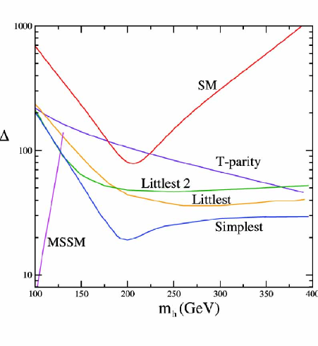
Figure 3: The finetuning measure for a variety of models [47].

Due to the quadratic divergence noted in eq(2) in the Standard Model, with a cutoff at the GUT scale, the fine tuning measure is $\Delta=O(10^{30})!$ This suggests that new physics is needed at a low scale but the nature of the new physics is limited by the need not to conflict with the successful precision tests of the Standard Model . Treating the Standard Model as an effective field theory below the cut-off scale there will be higher dimension operators involving the Standard Model fields suppressed by powers of the cut-off scale, $\Lambda.$ Assuming these operators appear unsuppressed, the minimum scale consistent with the precision tests is $\Lambda=10TeV.$ Using this cut-off one may calculate the residual fine tuning measure $\Delta=\left(\sum_{a}\Delta_{a}^{2}\right)^{1/2}$ in the Standard Model as a function of the Higgs mass. This is shown in Figure 3[47] by the curve labeled $SM,$ the dominant effect coming from the contribution to the Higgs mass from the top quark loop, and has $\Delta\geqslant 80.$ This residual need for fine tuning even if physics beyond the Standard Model is allowed is the “little hierarchy problem”.

To do better some of the new operators must be suppressed and this requires some symmetry to organise the corrections to the electroweak breaking scale so that they largely cancel. In the $MSSM$ supersymmetry plays this role and its fine tuning measure is also shown in Figure 3. One may see that $\Delta\geqslant 20$, the lowest tuning only applying for a Higgs close to its current mass limit. This is a significant improvement over the naive estimate using the low cut-off Standard Model and certainly a huge improvement over the GUT scale cut-off. Nonetheless the fact that $\Delta$ is still much larger than $1$ is worrying and much work has been done exploring ways of reducing the residual fine tuning. As we have seen the origin of the little hierarchy problem is the tension between the need to have the Higgs heavy, eq(30) and the need to keep the $Z$ light, eq(31). The latter equation follows from the radiative electroweak breaking c.f. eq(20) and so the little hierarchy problem raises doubts on the validity of this mechanism. For this reason we think it appropriate here to discuss briefly the attempts to eliminate this residual fine tuning.

In a supersymmetric context the residual fine tuning may be due to the choice of soft supersymmetry breaking parameters rather than the underlying supersymmetric theory itself. One may see from eq(31) that the gluino contribution proportional to $\,{M_{3}^{2}(0)}$ is particularly large. Reducing it reduces the fine tuning and this can be done in several ways. One can take a non-GUT symmetric form of the gaugino masses, reducing ${M_{3}^{2}(0)}$ relative to ${M_{1,2}^{2}(0).}$ Alternatively one can lower the scale at which the soft mass terms are defined (the messenger scale) thus reducing the magnitude of the logarithmic radiative terms responsible for the large coefficient of ${M_{3}^{2}(0)}$ and also adding new contributions to the quartic Higgs coupling. These changes can reduce the fine tuning needed, $\Delta\geqslant 10$ $\cite[cite]{[\@@bibref{}{Casas:2004uu}{}{}]},\cite[cite]{[\@@bibref{}{Chacko:2005ra}{}{}]}$ and even eliminate it in regions   of parameter space with $M_{\widetilde{\mathrm{t}}}$ small and $A_{t}$ large[50]. In schemes with anomaly mediation, although the initial spectrum is different, the fine tuning remains. An example of this called ”mirage unification” in which new SUSY breaking contributions from moduli solve the tachyonic slepton problem, has been studied in detail. Although it does reduce the gluino mass in simple versions of the model there is still significant fine tuning needed, $\Delta\geqslant 10^{3}$ $\cite[cite]{[\@@bibref{}{Lebedev:2005ge}{}{}]}.$ Another possibility, still in the context of supersymmetry, is to consider a more complicated scalar sector. This can affect the fine tuning needed, either by making the lightest Higgs invisible thus reducing the constraint on $M_{\mathrm{SUSY}}$ from the Higgs mass bounds, c.f. eq(30), or by adding new contributions to the quartic Higgs coupling which increase the tree level contribution to eq(30) and again reduce the constraint on $M_{\mathrm{SUSY}}.$ Again this only marginally improves the situation, $\Delta\geqslant 10\cite[cite]{[\@@bibref{}{Schuster:2005py}{}{}]}.$

What about the non-supersymmetric attempts to eliminate the little hierarchy problem? To do this it is necessary to have new contributions beyond the Standard Model ordered by a symmetry that prevent the radiative corrections to the Higgs mass becoming large, thus cancelling in part the top quark loop contribution. The only symmetry, apart from supersymmetry, capable of doing this is a (pseudo)Goldstone symmetry in which the components of the Standard Model Higgs doublet are Goldstone bosons associated with an underlying symmetry. It is known that the Standard Model gauge couplings do not respect such a symmetry and must give mass to the physical Higgs. However if the Goldstone symmetry is still unbroken at the level of the quadratically divergent radiative corrections there will be no Higgs mass corrections of the form of eq(2). In the little Higgs model [54] this is arranged to happen at one loop order, the leading radiative corrections to the Higgs mass occurring at logarithmic and finite order. To keep these latter contributions under control it is necessary that there are new physics contributions coming from states much lighter than the $10TeV$ cutoff assumed when calculating the fine tuning measure and beyond which some unspecified ultra-violet completion is assumed. The new physics contributions are needed to cancel the (irreducible) contribution of the top quark loop. In Figure 3 we show the resultant fine tuning for four representative little Higgs models (see reference [47] for details). In the littlest Higgs model the top contribution is largely cancelled by the contribution of a new ”top” quark, vector-like with respect to the Standard Model gauge group with a mass around $1TeV.$ One may see that there is still significant fine tuning needed, $\Delta\geqslant 40,$ with the lower values occurring only for a heavy Higgs which is difficult to reconcile with the precision tests of the Standard Model. The second little Higgs model and the $T-$parity little Higgs models are quite similar to the littlest Higgs model with small changes to the heavy spectrum and to the allowed couplings. As may be seen from the figure they do not change the fine tuning very much. The littlest Higgs model starts with a different symmetry group structure but still has a heavy top. For a heavy Higgs it improves on the fine tuning needed, $\Delta\geqslant 20,$ but does not eliminate the need for fine tuning. It is possible to build models protected by both a (pseudo)Goldstone symmetry and supersymmetry. Such models have double protection against large radiative corrections and can eliminate the fine tuning completely[53]. However the models are very complicated and it is hard to believe nature would go to such lengths to hide supersymmetry from us!

Given all this what conclusions can we draw from the little hierarchy problem? The first is that the non-supersymmetric attempts so far examined do not improve on the fine tuning needed even when comparing to the simplest MSSM scheme with a low Higgs mass. Moreover they do not attempt to provide an ultraviolet completion and thus do not address the question of a possible underlying unification of forces. On the other hand models with supersymmetry do provide an ultraviolet completion which allows for a stage of gauge or string unification at a high scale while separating the electroweak scale from the unification scale. For a low value of the Higgs mass the residual fine tuning needed is relatively modest, even in the simplest supersymmetric extensions of the Standard Model. There could also be relationships among the fundamental soft parameters in such a way that they should not be varied independently and hence the computed fine-tuning could be an overestimation (see e.g. the case with $\mu=-2M$ in ref.[31]). Given that these SM extensions lead to a very attractive picture of the theory at high scales in which the gauge couplings and soft masses unify and radiative electroweak breaking naturally explains the pattern of symmetry breaking in the Standard Model, we consider them to be very good candidates for extensions of the Standard Model. As we have discussed the residual fine tuning is sensitive to the soft supersymmetry breaking parameters and some reduction of fine tuning, even at higher Higgs mass, is possible without losing all the benefits of an underlying unification. As such they do provide an answer to the questions posed by the hierarchy problem and we think avoid the need to turn to more drastic ideas involving anthropic arguments[55], at least in what concerns the electroweak scale.

5 Summary and Prospects for SUSY and Higgs searches.

The need to solve the hierarchy problem is a strong motivation for low energy supersymmetry. Indeed the need to control radiative corrections means that supersymmetry is an essential ingredient of any viable string or GUT unification which unifies the gauge couplings at a very high scale. The fact that in the minimal supersymmetric extension of the Standard Model the prediction for gauge coupling unification is good to better than $1\%$ accuracy lends strong support to such supersymmetric unification. To complete the theory it is necessary to add soft supersymmetry breaking terms which must originate from a hidden sector. The radiative corrections that communicate the supersymmetry breaking lead naturally to a subsequent stage of gauge symmetry breaking at a low scale. Remarkably, for a heavy top quark, they naturally explain the pattern of symmetry breaking observed in the Standard Model, breaking the electroweak symmetry while leaving the symmetries associated with the strong and electromagnetic interactions unbroken.

The scale for the new SUSY particles is limited by our wish to solve the hierarchy problem to be in a range accessible to the LHC. The details of the spectrum depend on the detailed mechanism responsible for supersymmetry breaking. This in turn is limited by constraints from flavour changing neutral currents, electroweak symmetry breaking, dark matter abundance etc. What is interesting is that all these constraints can be satisfied in very simple supersymmetry breaking schemes and these schemes provide our ”best bet” for the physics Beyond the Standard Model. The archetypical model starts with the MSSM which has a stable LSP candidate for dark matter. Provided there are no additional gauge non singlet fields precision gauge unification is preserved suggesting mSUGRA mediated SUSY breaking as described below eq(9). The scheme has degenerate scalar masses, $m_{0},$ at a high scale so the flavour changing neutral currents are under control. A scan of parameter space shows that quite naturally the breaking of electroweak symmetry proceeds radiatively. Furthermore the dark matter abundance of the LSP can, for a limited parameter range, explain the dark matter abundance of the universe.

We find it remarkable that this simple favoured scheme is consistent with all know data. Moreover it is encouraging that it will be testable in the near future. Recent fits [14, 15, 16, 17, 18] to the parameters favours a solution in which the lightest Higgs is very light, with a distribution peaked around $M_{H}=115GeV$ and bounded by $M_{H}<127GeV,$ as is favoured by the need to minimise the little hierarchy problem, and close to the lower bound established by LEP and consistent with the precision tests of the Standard Model. In addition the SUSY breaking scale could be low corresponding to gluinos and other sparticles being readily produced at the LHC. The prospects are good that the LHC will not only be able to discover the Higgs, thus establishing the origin of mass, but also find supersymmetric states and open the way to establishing what lies  Beyond the Standard Model.

This work has been partially supported by CICYT (Spain), the Comunidad de Madrid (project HEPHACOS) and the European Commission under the RTN program MRTN-CT-2004-503369.

References

- [1] M. J. G. Veltman, Acta Phys. Polon. B 12 (1981) 437.
- [2] S. Ferrara, L. Girardello and F. Palumbo, Phys. Rev. D 20 (1979) 403.
- [3] L. E. Ibáñez and G. G. Ross, Phys. Lett. B 110 (1982) 215.
- [4] K. Inoue, A. Kakuto, H. Komatsu and S. Takeshita, Prog. Theor. Phys. 68, 927 (1982) [Erratum-ibid. 70, 330 (1983)].
- [5] L. Alvarez-Gaume, J. Polchinski and M. B. Wise, Nucl. Phys. B 221, 495 (1983).
- [6] J. R. Ellis, L. E. Ibáñez and G. G. Ross, Phys. Lett. B 113 (1982) 283.
-
[7]
A. H. Chamseddine, R. Arnowitt and P. Nath,
Phys. Rev. Lett. 49, 970 (1982);
L. E. Ibáñez, Phys. Lett. B 118, 73 (1982);
R. Barbieri, S. Ferrara and C. A. Savoy, Phys. Lett. B 119, 343 (1982);
L. J. Hall, J. Lykken and S. Weinberg, Phys. Rev. D 27, 2359 (1983). - [8] L. Alvarez-Gaume, M. Claudson and M. B. Wise, Nucl. Phys. B 207 (1982) 96; S. Dimopoulos and S. Raby, Nucl. Phys. B 219 (1983) 479; M. Dine and W. Fischler, Phys. Lett. B 110 (1982) 227.
- [9] L. E. Ibáñez and G. G. Ross, Phys. Lett. B 105 (1981) 439.
- [10] S. Dimopoulos, S. Raby and F. Wilczek, Phys. Rev. D 24 (1981) 1681; S. Dimopoulos and H. Georgi, Nucl. Phys. B 193, 150 (1981).
- [11] D. M. Ghilencea and G. G. Ross, Nucl. Phys. B 606 (2001) 101 [arXiv:hep-ph/0102306].
- [12] H. P. Nilles, Phys. Rept. 110, 1 (1984); J. A. Bagger, arXiv:hep-ph/9604232; S. P. Martin, arXiv:hep-ph/9709356. ; D. Bailin and A. Love, “Supersymmetric gauge field theory and string theory,” Institute of Physics publishing 1994; M. Drees, R. Godbole and P. Roy, “Theory and phenomenology of sparticles: An account of four-dimensional N=1 supersymmetry in high energy physics,”Cambridge University Press 2007; H. Baer and X. Tata, “Weak scale supersymmetry: From superfields to scattering events,” Cambridge University Press 2006; P.Binetruy, “Supersymmetry, Theory, Experiment and Cosmology”, Oxford University Press 2006.
- [13] F. Gabbiani, E. Gabrielli, A. Masiero and L. Silvestrini, Nucl. Phys. B 477, 321 (1996) [arXiv:hep-ph/9604387]; J. S. Hagelin, S. Kelley and T. Tanaka, Nucl. Phys. B 415, 293 (1994); T. Falk, K. A. Olive, M. Pospelov and R. Roiban, Nucl. Phys. B 560, 3 (1999) [arXiv:hep-ph/9904393]; S. Abel, S. Khalil and O. Lebedev, Nucl. Phys. B 606, 151 (2001) [arXiv:hep-ph/0103320].
- [14] J. R. Ellis, D. Nanopoulos, K. A. Olive and Y. Santoso, Phys. Lett. B 633 (2006) 583 [arXiv:hep-ph/0509331].
- [15] B. C. Allanach, Phys. Lett. B 635 (2006) 123 [arXiv:hep-ph/0601089].
- [16] J. R. Ellis, S. Heinemeyer, K. A. Olive and G. Weiglein, JHEP 0605 (2006) 005 [arXiv:hep-ph/0602220].
- [17] R. R. de Austri, R. Trotta and L. Roszkowski, JHEP 0605 (2006) 002 [arXiv:hep-ph/0602028].
- [18] J. Ellis, S. Heinemeyer, K. A. Olive and G. Weiglein, arXiv:hep-ph/0604180.
- [19] G. F. Giudice and R. Rattazzi, Phys. Rept. 322 (1999) 419 [arXiv:hep-ph/9801271].
- [20] L. Randall and R. Sundrum, Nucl. Phys. B 557 (1999) 79 [arXiv:hep-th/9810155]; G. F. Giudice, M. A. Luty, H. Murayama and R. Rattazzi, JHEP 9812 (1998) 027.
- [21] D. R. T. Jones and G. G. Ross, arXiv:hep-ph/0609210; R. Hodgson, I. Jack, D. R. T. Jones and G. G. Ross, Nucl. Phys. B 728, 192 (2005) [arXiv:hep-ph/0507193]; I. Jack and D. R. T. Jones, Phys. Lett. B 482, 167 (2000) [arXiv:hep-ph/0003081].
- [22] K. Choi, A. Falkowski, H. P. Nilles and M. Olechowski, Nucl. Phys. B 718, 113 (2005) [arXiv:hep-th/0503216]; O. Loaiza-Brito, J. Martin, H. P. Nilles and M. Ratz, AIP Conf. Proc. 805, 198 (2006) [arXiv:hep-th/0509158]; K. Choi, K. S. Jeong, T. Kobayashi and K. i. Okumura, Phys. Lett. B 633, 355 (2006) [arXiv:hep-ph/0508029]; R. Kitano and Y. Nomura, Phys. Lett. B 631, 58 (2005) [arXiv:hep-ph/0509039]; K. Choi, K. S. Jeong and K. i. Okumura, JHEP 0509, 039 (2005) [arXiv:hep-ph/0504037]; M. Endo, M. Yamaguchi and K. Yoshioka, Phys. Rev. D 72, 015004 (2005) [arXiv:hep-ph/0504036].
- [23] J. P. Derendinger, L. E. Ibanez and H. P. Nilles, Phys. Lett. B 155, 65 (1985); M. Dine, R. Rohm, N. Seiberg and E. Witten, Phys. Lett. B 156, 55 (1985).
- [24] V. S. Kaplunovsky and J. Louis, Phys. Lett. B 306, 269 (1993), arXiv:hep-th/9303040.
- [25] A. Brignole, L. E. Ibáñez and C. Muñoz, Nucl. Phys. B 422 (1994) 125, [Erratum-ibid. B 436 (1995) 747], arXiv:hep-ph/9308271.
- [26] P. G. Camara, L. E. Ibanez and A. M. Uranga, Nucl. Phys. B 689 (2004) 195, arXiv:hep-th/0311241; Nucl. Phys. B 708 (2005) 268; arXiv:hep-th/0408036.
- [27] J. A. Casas, A. Lleyda and C. Munoz, Phys. Lett. B 380 (1996) 59, arXiv:hep-ph/9601357.
- [28] S. A. Abel, B. C. Allanach, F. Quevedo, L. Ibanez and M. Klein, JHEP 0012 (2000) 026 [arXiv:hep-ph/0005260].
-
[29]
E. Cremmer, S. Ferrara, C. Kounnas and D. V. Nanopoulos,
Phys. Lett. B 133, 61 (1983) ;
J. R. Ellis, C. Kounnas and D. V. Nanopoulos, Nucl. Phys. B 247, 373 (1984). - [30] L. E. Ibáñez, Phys. Rev. D 71 (2005) 055005, arXiv:hep-ph/0408064.
- [31] B. C. Allanach, A. Brignole and L. E. Ibáñez, JHEP 0505 (2005) 030, arXiv:hep-ph/0502151.
-
[32]
D. Cremades, L. E. Ibáñez and F. Marchesano, JHEP
0307 (2003) 038, arXiv:hep-th/0302105];
F. Marchesano and G. Shiu, Phys. Rev. D 71 (2005) 011701, hep-th/0408059; JHEP 0411 (2004) 041, hep-th/0409132. - [33] D. Lüst, S. Reffert and S. Stieberger, hep-th/0410074.
- [34] L. E. Ibáñez, C. Muñoz and S. Rigolin, , Nucl. Phys. B553 (1999) 43, hep-ph/9812397; D. Lust, P. Mayr, R. Richter and S. Stieberger, arXiv:hep-th/0404134; B. Kors and P. Nath, Nucl. Phys. B 681 (2004) 77 arXiv:hep-th/0309167.
- [35] A. Font and L.E. Ibáñez, hep-th/0412150.
- [36] G. L. Kane, P. Kumar, J. D. Lykken and T. T. Wang, Phys. Rev. D 71 (2005) 115017, arXiv:hep-ph/0411125.
- [37] S. Kachru, R. Kallosh, A. Linde and S.P. Trivedi, Phys.Rev.D68(2003)046005, hep-th/0301240. For a recent review see M. R. Douglas and S. Kachru, arXiv:hep-th/0610102.
- [38] B. C. Allanach, F. Quevedo and K. Suruliz, JHEP 0604 (2006) 040, arXiv:hep-ph/0512081; J. P. Conlon, D. Cremades and F. Quevedo, arXiv:hep-th/0609180; S. Abdussalam, J.P. Conlon, F. Quevedo and K. Suruliz, arXiv:hep-th/06101XX
- [39] K. Choi, A. Falkowski, H. P. Nilles and M. Olechowski, Nucl. Phys. B 718 (2005) 113, arXiv:hep-th/0503216.
-
[40]
D. E. Diaconescu, B. Florea, S. Kachru and P. Svrcek, JHEP
0602 (2006) 020, arXiv:hep-th/0512170;
I. Garcia-Etxebarria, F. Saad and A. M. Uranga, JHEP 0608 (2006) 069, arXiv:hep-th/0605166. - [41] L. E. Ibanez and G. G. Ross, arXiv:hep-ph/9204201.
- [42] K. Inoue et al., Prog.Theor.Phys. 67 (1982) 1859.
- [43] L. E. Ibáñez and C. López, Phys. Lett. 126B, 54 (1984); Nucl. Phys. B 233, 511 (1984). L. E. Ibáñez, C. López and C. Muñoz, Nucl. Phys. B 256, 218 (1985).
- [44] H. E. Haber and R. Hempfling, Phys. Rev. Lett. 66, 1815 (1991); J. R. Ellis, G. Ridolfi and F. Zwirner, Phys. Lett. B 262, 477 (1991); Y. Okada, M. Yamaguchi and T. Yanagida, Phys. Lett. B 262, 54 (1991).
- [45] G. L. Kane and S. F. King, Phys. Lett. B 451, 113 (1999) [arXiv:hep-ph/9810374]; M. Bastero-Gil, G. L. Kane and S. F. King, Phys. Lett. B 474 (2000) 103 [arXiv:hep-ph/9910506].
- [46] R. Barbieri and G. F. Giudice, Nucl. Phys. B 306, 63 (1988).
- [47] J. A. Casas, J. R. Espinosa and I. Hidalgo, JHEP 0503 (2005) 038 [arXiv:hep-ph/0502066].
- [48] J. A. Casas, J. R. Espinosa and I. Hidalgo, arXiv:hep-ph/0402017.
- [49] Z. Chacko, Y. Nomura and D. Tucker-Smith, Nucl. Phys. B 725 (2005) 207 [arXiv:hep-ph/0504095].
- [50] R. Kitano and Y. Nomura, Phys. Lett. B 631 (2005) 58 [arXiv:hep-ph/0509039].
- [51] O. Lebedev, H. P. Nilles and M. Ratz, arXiv:hep-ph/0511320.
- [52] P. C. Schuster and N. Toro, arXiv:hep-ph/0512189.
- [53] A. Falkowski, S. Pokorski and M. Schmaltz, Phys. Rev. D 74 (2006) 035003 [arXiv:hep-ph/0604066]; A. Birkedal, Z. Chacko and M. K. Gaillard, JHEP 0410, 036 (2004) [arXiv:hep-ph/0404197]; P. H. Chankowski, A. Falkowski, S. Pokorski and J. Wagner, Phys. Lett. B 598, 252 (2004) [arXiv:hep-ph/0407242]; Z. Berezhiani, P. H. Chankowski, A. Falkowski and S. Pokorski, Phys. Rev. Lett. 96, 031801 (2006) [arXiv:hep-ph/0509311]; T. Roy and M. Schmaltz, JHEP 0601, 149 (2006) [arXiv:hep-ph/0509357]; C. Csaki, G. Marandella, Y. Shirman and A. Strumia, Phys. Rev. D 73, 035006 (2006) [arXiv:hep-ph/0510294].
- [54] N. Arkani-Hamed, A. Cohen and H. Georgi, Phys.lett.B513, 232, hep-th/0104005; N. Arkani-Hamed et al., 2002 JHEP 0208 021, hep-ph/0105239.
- [55] N. Arkani-Hamed and S. Dimopoulos, JHEP 0506, 073 (2005) [arXiv:hep-th/0405159]; G. F. Giudice and R. Rattazzi, Nucl. Phys. B 757, 19 (2006) [arXiv:hep-ph/0606105].