hep-ph/yymmnnn

A Collider Signature of the

Supersymmetric Golden Region

Maxim Perelstein and Christian Spethmann

Cornell Institute for High-Energy Phenomenology, Cornell University, Ithaca, NY 14853

Null results of experimental searches for the Higgs boson and the superpartners imply a certain amount of fine-tuning in the electroweak sector of the Minimal Supersymmetric Standard Model (MSSM). The “golden region” in the MSSM parameter space is the region where the experimental constraints are satisfied and the amount of fine-tuning is minimized. In this region, the stop trilinear soft term $A_{t}$ is large, leading to a significant mass splitting between the two stop mass eigenstates. As a result, the decay $\tilde{t}_{2}\to\tilde{t}_{1}Z$ is kinematically allowed throughout the golden region. We propose that the experiments at the Large Hadron Collider (LHC) can search for this decay through an inclusive signature, $Z+2j_{b}+\mbox{$E{\!\!\!\!}/_{T}$}+X$. We evaluate the Standard Model backgrounds for this channel, and identify a set of cuts that would allow detection of the supersymmetric contribution at the LHC for the MSSM parameters typical of the golden region. We also discuss other possible interpretations of a signal for new physics in the $Z+2j_{b}+\mbox{$E{\!\!\!\!}/_{T}$}+X$ channel, and suggest further measurements that could be used to distinguish among these interpretations.

1 Introduction

It is widely believed that physics at the TeV scale is supersymmetric. The simplest realistic implementation of this idea, the minimal supersymmetric standard model (MSSM) [1, 2], is the most popular extension of the standard model (SM). However, null results of experimental searches for the superpartners and, especially, the Higgs boson, place non-trivial constraints on the parameters of the model. Furthermore, the requirement that the observed electroweak symmetry breaking (EWSB) occur without significant fine-tuning places an additional constraint. It is well known that there is a certain amount of tension between these two constraints [3]. Several authors have interpreted this tension as a motivation to extend the minimal model [4], or to question the conventional ideas about naturalness [5]. An alternative interpretation, which we will explore in this paper, is that data and naturalness point to a particular ”golden” region within the parameter space of the minimal model, where the experimental bounds are satisfied and fine-tuning is close to the minimum value possible in the MSSM. This minimal value itself depends on the messenger scale of supersymmetry breaking $\Lambda_{\rm mess}$, determined by dynamics outside of the MSSM, in addition to the MSSM parameters. However, for any $\Lambda_{\rm mess}$, the points in the golden region require less fine-tuning compared to the rest of the MSSM parameter space. Thus, independently of the model of SUSY breaking, nature seems to provide us with a hint about what the MSSM parameters might be. In this paper, we will discuss experiments at the Large Hadron Collider (LHC) which will be able to determine whether this hint is correct.

Both the Higgs mass bound and naturalness considerations probe the effective Higgs potential, which is primarily determined by the parameters of the Higgs and top sectors of the MSSM. (The quantum part of the potential is dominated by the top/stop loops due to a large value of the top Yukawa coupling.) It is therefore these sectors that are most directly constrained by data. We will focus on collider measurements probing these sectors.

The golden region is characterized by relatively small values of the $\mu$ parameter and the stop soft masses $m_{Q^{3}}$, $m_{u^{3}}$ (both are required to minimize fine-tuning of the $Z$ mass), and a large stop trilinear soft term $A_{t}$ (required to raise the Higgs mass above the LEP2 lower bound). The spectrum is then expected to contain light neutralinos and charginos with a substantial higgsino content, as well as two light (sub-TeV) stop mass eigenstates, $\tilde{t}_{1}$ and $\tilde{t}_{2}$, with a large (typically a few hundered GeV) mass splitting. A striking consequence of such a “split stop” spectrum is that the decay

$$\tilde{t}_{2}\to\tilde{t}_{1}+Z$$ (1)

is kinematically allowed. Observing this decay at the LHC would provide clear evidence that the stop mass difference is larger than the $Z$ mass, and studying the $Z$ distributions would provide an approximate measurement of this quantity. In this paper, we will argue that the decay (1) should be observable at the LHC, with realistic integrated luminosity, for the MSSM parameters in the golden region.

The experimental signature of the decay (1) depends on the decay pattern of the $\tilde{t}_{1}$. Since stops are almost always pair-produced at the LHC, it also depends on how the second $\tilde{t}_{2}$ decays. The details of both decay patterns depend on the superpartner spectrum. However, both $\tilde{t}_{1}$ and $\tilde{t}_{2}$ decay products always contain a $b$ quark, produced either directly or through a top decay, as well as (under the usual assumptions of conserved R parity and weakly interacting lightest supersymmetric particle) large missing transverse energy. We therefore propose an inclusive final state

$$Z+2j_{b}+\mbox{$E{\!\!\!\!}/_{T}$}+X,$$ (2)

where $Z$ is assumed to be reconstructed from leptonic decays and $j_{b}$ denotes a $b$ jet, as a signature of the $\tilde{t}_{2}\tilde{t}_{2}^{*}$ production followed by the decay (1).

Throughout the golden region of the MSSM, both the $\tilde{t}_{2}$ pair-production cross section and the branching fraction of the decay (1) are sizeable. Therefore, a null result of a search for a non-SM contribution in the channel (2) would provide a strong argument against this scenario. Unfortunately, a positive identification of non-SM physics in this channel would not necessarily imply that the stops are split. Indeed, in the MSSM, events in this channel may appear even if the decay (1) is kinematically forbidden, since $Z$ bosons may also be produced in decays of neutralinos and charginos [12]. For example, a cascade

$$\tilde{b}\to b\chi_{2}^{0},~{}~{}~{}\chi_{2}^{0}\to Z\chi_{1}^{0},$$ (3)

or a similar cascade with charginos replacing the neutralinos, gives the signature (2). Distinguishing these interpretations is difficult, and there is no single “silver bullet” observable that would remove this ambiguity. However, a variety of measurements can be used to shed light on this question (see Section 5), and combining all available evidence may allow one to build a convincing case for (or against) the interpretation of the signature (2) in terms of the decay (1).

The paper is organized as follows. In Section 2, we review the fine-tuning and Higgs mass constraints in the MSSM, as well as other experimental results that determine the shape of the golden region. In Section 3, we define a benchmark point which is characteristic of the golden region and suitable for studying its collider phenomenology. Section 4 is dedicated to a detailed analysis of the observability of the $Z+2j_{b}+\mbox{$E{\!\!\!\!}/_{T}$}$ signature, including a study of the SM backgrounds. In Section 5, we discuss the alternative interpretations of this signature within the MSSM, and outline the measurements that would need to be performed to discriminate between these interpretations. Section 6 contains our conclusions, and outlines some possible directions for future work.

2 The Golden Region

In this section, we will discuss the constraints on the MSSM parameters imposed by current experimental data and naturalness, focusing on the Higgs and top sectors. Our goal is to understand the qualitative features of the MSSM golden region, rather than to determine the precise location of its boundaries which are in any case fuzzy due to an inherent lack of precision surrounding the concept of fine-tuning. With this motivation, we will make several approximations which greatly clarify the picture.

Phenomenological studies of the MSSM are complicated by the large number of free parameters. Typically, studies are performed within simplified frameworks, which assume certain correlations among the parameters motivated by high-scale unification and/or by specific models of SUSY breaking. However, the shape of the golden region is to a great extent independent of such assumptions. The Higgs sector of the MSSM is strongly coupled to the top sector, but couplings to the rest of the MSSM are weaker. One may therefore begin by considering the Higgs and top sectors in isolation; that is, the gauge and non-top Yukawa couplings are set to zero. In this approximation, physics is described in terms of the holomorphic Higgs mass $\mu$ and the six parameters appearing in the soft Lagrangian for the Higgs and top sectors:

$${\cal L}\,=\,-m_{u}^{2}|H_{u}|^{2}-m_{d}^{2}|H_{d}|^{2}-\left(bH_{u}^{T}H_{d}+{\rm c.c.}\right)-m_{Q^{3}}^{2}Q^{3\dagger}Q^{3}-m_{u^{3}}^{2}|u^{3}|^{2}-\left(y_{t}A_{t}Q^{3\dagger}H_{u}u^{3}+{\rm c.c.}\right),$$ (4)

where $y_{t}$ is the MSSM top Yukawa coupling, $y_{t}=y_{t}^{\rm SM}/\sin\beta$. Since the model has to reproduce the known EWSB scale, $v=174$ GeV, only six parameters are independent. We choose the physical basis:

$$\tan\beta,\mu,m_{A},\tilde{m}_{1},\tilde{m}_{2},\theta_{t},$$ (5)

where $m_{A}$ is the CP-odd Higgs mass, $\tilde{m}_{1}$ and $\tilde{m}_{2}$ are stop eigenmasses (by convention, $\tilde{m}_{2}>\tilde{m}_{1}$) and $\theta_{t}$ is the stop mixing angle. We will analyze the fine-tuning and Higgs mass constraints in this approximation and map out the golden region in the six-parameter space (5).

Before proceeding, let us discuss the sizes of contributions to the relevant observables that are omitted in this approximation scheme. The leading contributions to the Higgs effective potential due to the $SU(3)$, $SU(2)$ and $U(1)_{Y}$ gauge interactions and the bottom Yukawa coupling are expected to be of the order

$$\frac{g_{3}^{2}M_{3}^{2}}{16\pi^{2}\lambda_{t}^{2}M_{\tilde{t}}^{2}},~{}~{}~{}\frac{g_{2}^{2}M_{2}^{2}}{\lambda_{t}^{2}M_{\tilde{t}}^{2}},~{}~{}~{}\frac{g_{1}^{2}M_{1}^{2}}{\lambda_{t}^{2}M_{\tilde{t}}^{2}},~{}~{}~{}\frac{m_{b}^{2}M_{\tilde{b}}^{2}\tan^{2}\beta}{m_{t}^{2}M_{\tilde{t}}^{2}},$$ (6)

respectively, compared to the one-loop top sector contribution. Here $g_{i}$ and $M_{i}$ are the gauge couplings and (weak-scale) gaugino masses for each group, and $M_{\tilde{t}}$ is the stop mass scale, which can be conveniently taken as the average between the two stop eigenmasses. (The same definition can be made for $M_{\tilde{b}}$ if sbottoms are non-degenerate.) For a wide range of sensible superpartner spectra, these corrections are subdominant: this is the case if

$$M_{1}/M_{\tilde{t}}\mathrel{\mathchoice{\lower 2.5pt\vbox{\halign{$\mathsurround 0pt\displaystyle\hfil#\hfil$\cr<\crcr\sim\crcr}}}{\lower 2.5pt\vbox{\halign{$\mathsurround 0pt\textstyle\hfil#\hfil$\cr<\crcr\sim\crcr}}}{\lower 2.5pt\vbox{\halign{$\mathsurround 0pt\scriptstyle\hfil#\hfil$\cr<\crcr\sim\crcr}}}{\lower 2.5pt\vbox{\halign{$\mathsurround 0pt\scriptscriptstyle\hfil#\hfil$\cr<\crcr\sim\crcr}}}}4,~{}~{}M_{2}/M_{\tilde{t}}\mathrel{\mathchoice{\lower 2.5pt\vbox{\halign{$\mathsurround 0pt\displaystyle\hfil#\hfil$\cr<\crcr\sim\crcr}}}{\lower 2.5pt\vbox{\halign{$\mathsurround 0pt\textstyle\hfil#\hfil$\cr<\crcr\sim\crcr}}}{\lower 2.5pt\vbox{\halign{$\mathsurround 0pt\scriptstyle\hfil#\hfil$\cr<\crcr\sim\crcr}}}{\lower 2.5pt\vbox{\halign{$\mathsurround 0pt\scriptscriptstyle\hfil#\hfil$\cr<\crcr\sim\crcr}}}}2,~{}~{}M_{3}/M_{\tilde{t}}\mathrel{\mathchoice{\lower 2.5pt\vbox{\halign{$\mathsurround 0pt\displaystyle\hfil#\hfil$\cr<\crcr\sim\crcr}}}{\lower 2.5pt\vbox{\halign{$\mathsurround 0pt\textstyle\hfil#\hfil$\cr<\crcr\sim\crcr}}}{\lower 2.5pt\vbox{\halign{$\mathsurround 0pt\scriptstyle\hfil#\hfil$\cr<\crcr\sim\crcr}}}{\lower 2.5pt\vbox{\halign{$\mathsurround 0pt\scriptscriptstyle\hfil#\hfil$\cr<\crcr\sim\crcr}}}}10,~{}~{}M_{\tilde{b}}\mathrel{\mathchoice{\lower 2.5pt\vbox{\halign{$\mathsurround 0pt\displaystyle\hfil#\hfil$\cr<\crcr\sim\crcr}}}{\lower 2.5pt\vbox{\halign{$\mathsurround 0pt\textstyle\hfil#\hfil$\cr<\crcr\sim\crcr}}}{\lower 2.5pt\vbox{\halign{$\mathsurround 0pt\scriptstyle\hfil#\hfil$\cr<\crcr\sim\crcr}}}{\lower 2.5pt\vbox{\halign{$\mathsurround 0pt\scriptscriptstyle\hfil#\hfil$\cr<\crcr\sim\crcr}}}}\frac{35M_{\tilde{t}}}{\tan\beta}.$$ (7)

The following discussion is valid for spectra obeying these constraints. If some of the above inequalities are violated, the analysis could be easily extended to include the corresponding effects; however, little additional insight would be gained.

2.1 Constraints on the Higgs Sector

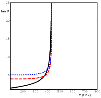
Figure 1: Contours of 1% fine-tuning in the ($\mu,\tan\beta$) plane. The black (solid) contour corresponds to $m_{A}=100$ GeV, but remains essentially unchanged for any value of $m_{A}$ in the range between 100 and 1000 GeV. The red (dashed) and blue (dotted) contours correspond to $m_{A}=1.5$ and 2 TeV, respectively.

At tree level, the $Z$ mass in the MSSM is given by

$$m_{Z}^{2}\,=\,-m_{u}^{2}\left(1-\frac{1}{\cos 2\beta}\right)-m_{d}^{2}\left(1+\frac{1}{\cos 2\beta}\right)-2|\mu|^{2}\,,$$ (8)

where

$$\sin 2\beta=\frac{2b}{m_{u}^{2}+m_{d}^{2}+2|\mu|^{2}}\,.$$ (9)

Following Barbieri and Guidice [13], we quantify fine-tuning by computing

$$A(\xi)\,=\,\left|\frac{\partial\log m_{Z}^{2}}{\partial\log\xi}\right|,$$ (10)

where $\xi=m_{u}^{2},m_{d}^{2},b,\mu$ are the relevant Lagrangian parameters. In terms of the physical parameters (5), we obtain

$$A(\mu) = \frac{4\mu^{2}}{m_{Z}^{2}}\,\left(1+\frac{m_{A}^{2}+m_{Z}^{2}}{m_{A}^{2}}\tan^{2}2\beta\right),$$

$$A(b) = \left(1+\frac{m_{A}^{2}}{m_{Z}^{2}}\right)\tan^{2}2\beta,$$

$$A(m_{u}^{2}) = \left|\frac{1}{2}\cos 2\beta+\frac{m_{A}^{2}}{m_{Z}^{2}}\cos^{2}\beta-\frac{\mu^{2}}{m_{Z}^{2}}\right|\times\left(1-\frac{1}{\cos 2\beta}+\frac{m_{A}^{2}+m_{Z}^{2}}{m_{A}^{2}}\tan^{2}2\beta\right),$$

$$A(m_{d}^{2}) = \left|-\frac{1}{2}\cos 2\beta+\frac{m_{A}^{2}}{m_{Z}^{2}}\sin^{2}\beta-\frac{\mu^{2}}{m_{Z}^{2}}\right|\times\left|1+\frac{1}{\cos 2\beta}+\frac{m_{A}^{2}+m_{Z}^{2}}{m_{A}^{2}}\tan^{2}2\beta\right|,$$

where we assumed $\tan\beta>1$. The overall fine-tuning $\Delta$ is defined by adding the four $A$’s in quadruture; values of $\Delta$ far above one indicate fine-tuning. For concreteness, we will require $\Delta\leq 100$, corresponding to fine tuning of 1% or better. This requirement maps out the golden region in the space of $(\tan\beta,\mu,M_{A})$, as illustrated in figure 1. (We do not plot $\mu<100$ GeV, since this region is ruled out by LEP2 chargino searches.) The shape of this region is easily understood. In the limit of large $\tan\beta$, the parameters $A(m_{u}^{2})$ and $A(m_{d}^{2})$ are small, and $A(\mu)$ and $A(b)$ (considered separately) lead to constraints

$$\frac{\mu}{m_{Z}}<\frac{\Delta_{\rm max}^{1/2}}{2},~{}~{}~{}\frac{m_{A}}{m_{Z}}<\frac{\Delta_{\rm max}^{1/2}}{2}\,\tan\beta\,,$$ (12)

which are clearly reflected in Fig. 1. As $\beta$ approaches $\pi/4$, the factors of $1/\cos 2\beta$ and $\tan 2\beta$, present in all four $A$ parameters, become large, and as a result the model is always fine-tuned for $\tan\beta\mathrel{\mathchoice{\lower 2.5pt\vbox{\halign{$\mathsurround 0pt\displaystyle\hfil#\hfil$\cr<\crcr\sim\crcr}}}{\lower 2.5pt\vbox{\halign{$\mathsurround 0pt\textstyle\hfil#\hfil$\cr<\crcr\sim\crcr}}}{\lower 2.5pt\vbox{\halign{$\mathsurround 0pt\scriptstyle\hfil#\hfil$\cr<\crcr\sim\crcr}}}{\lower 2.5pt\vbox{\halign{$\mathsurround 0pt\scriptscriptstyle\hfil#\hfil$\cr<\crcr\sim\crcr}}}}2$.

2.2 Constraints on the Top Sector

Naturalness also constrains the size of the quantum corrections to the parameters in Eq. (8). The largest correction in the MSSM is the one-loop contribution to the $m_{u}^{2}$ parameter from top and stop loops:

$$\delta m_{H_{u}}^{2} \approx \frac{3y_{t}^{2}}{16\pi^{2}}\left(\tilde{m}^{2}_{Q_{3}}+\tilde{m}^{2}_{t^{c}}+A_{t}^{2}\right)\,\log\frac{2\Lambda^{2}}{\tilde{m}^{2}_{Q_{3}}+\tilde{m}^{2}_{t^{c}}}$$ (13)

$$\approx \frac{3}{16\pi^{2}}\left(y_{t}^{2}\left(\tilde{m}_{1}^{2}+\tilde{m}_{2}^{2}-2m_{t}^{2}\right)+\frac{(\tilde{m}_{2}^{2}-\tilde{m}_{1}^{2})^{2}}{4v^{2}\sin^{2}\beta}\sin^{2}2\theta_{t}\right)\,\log\frac{2\Lambda^{2}}{\tilde{m}_{1}^{2}+\tilde{m}_{2}^{2}}\,,$$

where $m_{t}$ is the top mass, $\Lambda$ is the scale at which the logarithmic divergence is cut off, and finite (matching) corrections have been ignored. In the second line, we re-expressed the correction in terms of the physical (tree-level) stop masses, assuming $A_{t}\gg\mu/\tan\beta$ (as will always be the case in this study). The correction induced by this effect in the $Z$ mass is

$$\delta_{t}m_{Z}^{2}\approx-\delta m_{H_{u}}^{2}\left(1-\frac{1}{\cos 2\beta}\right),$$ (14)

where we ignored the renormalization of the angle $\beta$ by top/stop loops: the contribution of this effect scales as $1/\tan^{2}\beta$ and is subdominant for $\tan\beta\mathrel{\mathchoice{\lower 2.5pt\vbox{\halign{$\mathsurround 0pt\displaystyle\hfil#\hfil$\cr>\crcr\sim\crcr}}}{\lower 2.5pt\vbox{\halign{$\mathsurround 0pt\textstyle\hfil#\hfil$\cr>\crcr\sim\crcr}}}{\lower 2.5pt\vbox{\halign{$\mathsurround 0pt\scriptstyle\hfil#\hfil$\cr>\crcr\sim\crcr}}}{\lower 2.5pt\vbox{\halign{$\mathsurround 0pt\scriptscriptstyle\hfil#\hfil$\cr>\crcr\sim\crcr}}}}2$. To measure the fine-tuning between the bare (tree-level) and one-loop contributions, we introduce

$$\Delta_{t}\,=\,\left|\frac{\delta_{t}m_{Z}^{2}}{m_{Z}^{2}}\right|.$$ (15)

Choosing the maximum allowed value of $\Delta_{t}$ selects a region in the stop sector parameter space, $(\tilde{m}_{1},\tilde{m}_{2},\theta_{t})$, whose shape is approximately independent of the other parameters. This constraint is shown by the black (dashed) lines in Figs. 2, where we plot 5%, 3%, 1% and 0.5% tuning contours (corresponding to $\Delta_{t}=20,33.3,100$, and 200, respectively) in the stop mass plane for several values of $\theta_{t}$ and $\tan\beta=10$. Note that the particular values of $\Delta_{t}$ depend on the scale $\Lambda$; we choose it to be 100 TeV in this figure. However, the shape of the contours and the obvious trend for tuning to increase with the two stop masses is independent of $\Lambda$.

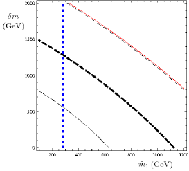
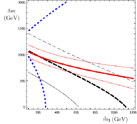
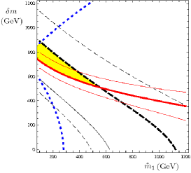
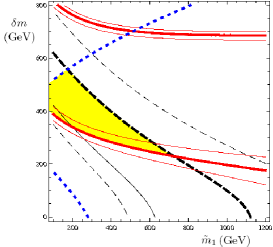
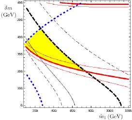
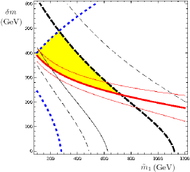
Figure 2: Fine-tuning (black/dashed contours), Higgs mass bound (red/colid contours), and $\rho$-parameter (blue/dotted contours) constraints in the ($\tilde{m}_{1}$, $\delta m$) plane. The six panels correspond to (starting from the upper-left corner, clockwise): $\theta_{t}=0,\pi/25,\pi/15,\pi/6,\pi/4,\pi/3$. In all panels $\tan\beta=10$. The yellow/shaded intersection of the regions allowed by the three constraints is the MSSM “golden” region.

The second constraint that determines the shape of the golden region is the LEP2 lower bound on the Higgs mass [14]. For generic MSSM parameter values, the limit on the lightest CP-even Higgs is very close to that for the SM Higgs:

$$m(h^{0})\mathrel{\mathchoice{\lower 2.5pt\vbox{\halign{$\mathsurround 0pt\displaystyle\hfil#\hfil$\cr>\crcr\sim\crcr}}}{\lower 2.5pt\vbox{\halign{$\mathsurround 0pt\textstyle\hfil#\hfil$\cr>\crcr\sim\crcr}}}{\lower 2.5pt\vbox{\halign{$\mathsurround 0pt\scriptstyle\hfil#\hfil$\cr>\crcr\sim\crcr}}}{\lower 2.5pt\vbox{\halign{$\mathsurround 0pt\scriptscriptstyle\hfil#\hfil$\cr>\crcr\sim\crcr}}}}114~{}{\rm GeV}.$$ (16)

It is possible for a lighter Higgs (down to about 90 GeV) to be consistent with the negative results of the LEP2 searches; however, this requires precise coincidence between $m(h^{0})$ and $m_{A}$, which should be regarded as additional source of fine-tuning. Thus, we will use the LEP2 bound for the SM Higgs [15], 114.4 GeV, as the lower bound on $m(h^{0})$ in this analysis. At tree level, the MSSM predicts $m(h^{0})\leq m_{Z}|\cos 2\beta|$, and large loop corrections are required to satisfy this bound. Extensive calculations of these corrections have been performed in the literature (for a recent summary of the status of these calculations, see Ref. [16]). Complete one-loop corrections within the MSSM are known. The dominant one-loop contribution is from top and stop loops; for $\tan\beta\mathrel{\mathchoice{\lower 2.5pt\vbox{\halign{$\mathsurround 0pt\displaystyle\hfil#\hfil$\cr>\crcr\sim\crcr}}}{\lower 2.5pt\vbox{\halign{$\mathsurround 0pt\textstyle\hfil#\hfil$\cr>\crcr\sim\crcr}}}{\lower 2.5pt\vbox{\halign{$\mathsurround 0pt\scriptstyle\hfil#\hfil$\cr>\crcr\sim\crcr}}}{\lower 2.5pt\vbox{\halign{$\mathsurround 0pt\scriptscriptstyle\hfil#\hfil$\cr>\crcr\sim\crcr}}}}35$, the sbottom loop contribution is also important. The two-loop corrections to these contributions from strong and Yukawa interactions are also known. Numerical packages incorporating these results are available [17, 18]. For our purposes here, however, it is convenient to use a simple analytic approximation, due to Carena et. al. [19], which includes the one-loop and leading-log two-loop contributions from top and stop loops:

$$m^{2}(h^{0}) = m_{Z}^{2}\cos^{2}2\beta\,\left(1-\frac{3}{8\pi^{2}}\frac{m_{t}^{2}}{v^{2}}\,t\right)$$ (17)

$$+ \frac{3}{4\pi^{2}}\frac{m_{t}^{4}}{v^{2}}\left[\frac{1}{2}X_{t}+t+\frac{1}{16\pi^{2}}\left(\frac{3}{2}\frac{m_{t}^{2}}{v^{2}}-32\pi\alpha_{3}\right)\left(X_{t}t+t^{2}\right)\right]\,,$$

where $\alpha_{3}$ is the strong coupling constant evaluated at the pole top quark mass $M_{t}$; $m_{t}=M_{t}/(1+\frac{4}{3\pi}\alpha_{3})$ is the on-shell top mass; and

$$X_{t} = \frac{2(A_{t}-\mu\cot\beta)^{2}}{M_{\rm susy}^{2}}\,\left(1-\frac{(A_{t}-\mu\cot\beta)^{2}}{12M_{\rm susy}^{2}}\right)\,,$$

$$t = \log\frac{M_{\rm susy}^{2}}{M_{t}^{2}}.$$ (18)

The scale $M_{\rm susy}^{2}$ is defined as the arithmetical average of the diagonal elements of the stop mass matrix. The expression (17) is valid when the masses of all superparticles, as well as the CP-odd Higgs mass $m_{A}$, are of order $M_{\rm susy}$. Additional threshold corrections may be required, for example, if $m_{A}<M_{\rm susy}$; for simplicity, we will ignore such corrections here. Eq. (17) agrees with the state-of-the-art calculations to within a few GeV for typical MSSM parameters [16]; while such accuracy is clearly inadequate for precision studies, it is sufficient for the present analysis.

The contours in the stop mass plane corresponding to the LEP2 Higgs mass bound are superimposed on the fine-tuning contours in Figs. 2. The positions of these contours depend strongly on the top quark mass. We used $M_{t}=171.4\pm 2.1$ GeV [20], and plotted the constraint corresponding to the central value (thick red/solid lines), as well as the boundaries of the 95% c.l. band (thinner red/solid lines). The contours are approximately independent of $\tan\beta$ for $3\mathrel{\mathchoice{\lower 2.5pt\vbox{\halign{$\mathsurround 0pt\displaystyle\hfil#\hfil$\cr<\crcr\sim\crcr}}}{\lower 2.5pt\vbox{\halign{$\mathsurround 0pt\textstyle\hfil#\hfil$\cr<\crcr\sim\crcr}}}{\lower 2.5pt\vbox{\halign{$\mathsurround 0pt\scriptstyle\hfil#\hfil$\cr<\crcr\sim\crcr}}}{\lower 2.5pt\vbox{\halign{$\mathsurround 0pt\scriptscriptstyle\hfil#\hfil$\cr<\crcr\sim\crcr}}}}\tan\beta\mathrel{\mathchoice{\lower 2.5pt\vbox{\halign{$\mathsurround 0pt\displaystyle\hfil#\hfil$\cr<\crcr\sim\crcr}}}{\lower 2.5pt\vbox{\halign{$\mathsurround 0pt\textstyle\hfil#\hfil$\cr<\crcr\sim\crcr}}}{\lower 2.5pt\vbox{\halign{$\mathsurround 0pt\scriptstyle\hfil#\hfil$\cr<\crcr\sim\crcr}}}{\lower 2.5pt\vbox{\halign{$\mathsurround 0pt\scriptscriptstyle\hfil#\hfil$\cr<\crcr\sim\crcr}}}}35$; the golden region shrinks rapidly outside of this range of $\tan\beta$. We use $\tan\beta=10$ in the plots. The overlap between the regions of acceptably low fine-tuning (for definiteness, we choose $\Delta_{t}=100$) and experimentally allowed Higgs mass defines the golden region, shaded in yellow in Figs. 2.

2.3 Collider Bounds, Precision Electroweak Constraints and Rare Decays

Apart from the Higgs mass bound, several other observables constrain the shape of the golden region.

First, direct collider bounds play a role in determining the boundary at low $\mu$ and $\tilde{m}_{1}$: LEP2 searches for direct production of charginos and stops constrain both $\mu$ and $\tilde{m}_{1}$ to be above $\approx 100$ GeV, and are to a large extent independent of the rest of the MSSM parameters. (At large $\tan\beta$, it can be easily shown that $m(\chi^{\pm}_{1})<|\mu|$ for any $M_{2}$.) The Tevatron stop searches yield a similar (though more model-dependent) bound on $\tilde{m}_{1}$. A sbottom search in the $b\chi_{1}^{0}$ channel (which is relevant because the $\tilde{b}_{L}$ mass is given by $m_{Q^{3}}$, and can be expressed in terms of $\tilde{m}_{1}$ and $\tilde{m}_{2}$) places a lower bound $m(\tilde{b}_{L})\geq 200$ GeV. However, this bound will not be used in our analysis since it is highly sensitive to the neutralino mass and can be easily evaded if $m(\chi_{1}^{0})>80$ GeV.

Second, in the presence of a large $A_{t}$ term, stop and sbottom loops may induce a significant correction to the $\rho$ parameter. This correction is known at the two-loop level [21]; for our purposes, it suffices to use the one-loop result:

$$\Delta\rho\,=\,\frac{3G_{F}}{8\sqrt{2}\pi^{2}}\left(-\sin\theta_{t}^{2}\cos\theta_{t}^{2}F_{0}(\tilde{m}_{1}^{2},\tilde{m}_{2}^{2})+\cos^{2}\theta_{t}F_{0}(\tilde{m}_{1}^{2},m_{\tilde{b}_{L}}^{2})+\sin^{2}\theta_{t}F_{0}(\tilde{m}_{2}^{2},m_{\tilde{b}_{L}}^{2})\right)\,,$$ (19)

where

$$F_{0}(a,b)\,=\,a+b-\frac{2ab}{a-b}\log\frac{a}{b}.$$ (20)

Expressing $m_{\tilde{b}_{L}}$ in terms of $\tilde{m}_{1}$, $\tilde{m}_{2}$ and $\theta_{t}$, and using the PDG value $\rho=1.0002\begin{array}[]{l}\scriptstyle+0.0004\\[-6.45831pt] \scriptstyle-0.0007\end{array}$ [15], we obtain the 95% c.l. contours in the stop mass plane shown by the blue/dotted lines in Figs. 2. This constraint eliminates a part of the parameter space with very low $\tilde{m}_{1}$ and large $\delta m$.

Finally, several low-energy measurements play a role in constraining the MSSM parameter space; among these, the $b\to s\gamma$ decay rate [22] and the anomalous magnetic moment of the muon, $g_{\mu}-2$ [23], provide the most stringent constraints. The supersymmetric contribution to $g_{\mu}-2$ depends sensitively on the slepton and weak gaugino mass scales, and only weakly on the parameters defining the golden region. On the other hand, since the golden spectrum contains light stops and higgsinos, we can expect a large contribution to the $b\to s\gamma$ rate from the $\tilde{t}-\tilde{H}$ loop. It is well known, however, that this can be cancelled by the contribution of the top-charged Higgs loop. A simplified analysis of this constraint based on the one-loop analytic formulas presented in Ref. [24] shows that for any values of the stop masses inside the golden region in Figs. 2, and for any value of $\mu$ between 100 and 500 GeV, one can find values of $m_{A}$ in the 100-1000 GeV range for which this cancellation ensures consistency with experiment. (Recall that $m^{2}(H^{\pm})=m_{A}^{2}+m_{W}^{2}$.) For low $\tilde{m}_{1}$ and $\mu$, however, the cancellation only occurs in a narrow band of $m_{A}$, which can be thought of as an additional source of fine tuning. A detailed analysis of this issue is outside the scope of this paper.

3 A Benchmark Point for Collider Studies

The analysis of Section 2 defined the golden region in the six-dimensional parameter space (5); its shape is approximately independent of the other MSSM parameters. This region has the following interesting qualitative features:

• Both stops typically have masses below $1$ TeV;

• A substantial mass splitting between the two stop quarks is required: typically,
  $\delta m\mathrel{\mathchoice{\lower 2.5pt\vbox{\halign{$\mathsurround 0pt\displaystyle\hfil#\hfil$\cr>\crcr\sim\crcr}}}{\lower 2.5pt\vbox{\halign{$\mathsurround 0pt\textstyle\hfil#\hfil$\cr>\crcr\sim\crcr}}}{\lower 2.5pt\vbox{\halign{$\mathsurround 0pt\scriptstyle\hfil#\hfil$\cr>\crcr\sim\crcr}}}{\lower 2.5pt\vbox{\halign{$\mathsurround 0pt\scriptscriptstyle\hfil#\hfil$\cr>\crcr\sim\crcr}}}}200$ GeV;

• The stop mixing angle must be non-zero: there is no intersection between the naturalness and Higgs mass constraints for $\theta_{t}=0,\pi/2$.

$m_{Q^{3}}$	$m_{u^{3}}$	$m_{d^{3}}$	$A_{t}$	$\mu$	$m_{A}$	$\tan\beta$	$M_{1}$	$M_{2}$	$M_{3}$	$m_{\tilde{q}}$	$m_{\tilde{\ell}}$
548.7	547.3	1000	1019	250	200	10	1000	1000	1000	1000	1000

Table 1: The benchmark point: MSSM input parameters, defined at the weak scale. (All dimensionful parameters are in GeV.)

The first feature implies that both $\tilde{t}_{1}$ and $\tilde{t}_{2}$ will be produced with sizeable cross sections at the LHC, so that the stop sector can be studied directly experimentally. The second feature implies that the decay mode $\tilde{t}_{2}\to\tilde{t}_{1}Z$ is kinematically allowed. The vertex responsible for this decay is given by

$$\frac{1}{2}\sin 2\theta_{t}\,\frac{g}{c_{w}}\,\left(\frac{1}{2}-\frac{4}{3}s_{w}^{2}\right),$$ (21)

where $c_{w}$ and $s_{w}$ are the cosine and sine of the SM Weinberg angle. The last of the three points above then guarantees that the vertex is non-zero, and the decay $\tilde{t}_{2}\to\tilde{t}_{1}Z$ indeed occurs.

$\tilde{m}_{1}$	$\tilde{m}_{2}$	$m_{\tilde{b}_{L}}$	$m(\chi_{1}^{0})$	$m(\chi_{2}^{0})$	$m(\chi_{1}^{\pm})$	$m_{h^{0}}$	$m_{H^{0}}$	$m_{A}$	$m_{H^{\pm}}$
400	700	552	243	253	247	128.6	201	200	250

Table 2: The benchmark point: physical spectrum. All masses are in GeV. The masses of the superparticles not listed here are close to 1 TeV.

The branching ratio of the $\tilde{t}_{2}\to\tilde{t}_{1}Z$ mode depends on which competing $\tilde{t}_{2}$ decay channels are available. The possible two-body channels are

$$t\tilde{g},~{}~{}~{}t\tilde{\chi^{0}},~{}~{}~{}b\tilde{\chi^{+}}\,,~{}~{}~{}\tilde{b}W^{+},~{}~{}~{}\tilde{b}H^{+},~{}~{}~{}\tilde{t}_{1}h^{0},~{}~{}~{}\tilde{t}_{1}H^{0},~{}~{}~{}\tilde{t}_{1}A^{0}\,,$$ (22)

where $\tilde{\chi^{0}}$ and $\tilde{\chi^{+}}$ denote all the neutralinos and charginos that are kinematically accessible, and flavor-changing couplings are assumed to be negligible.

We would like to evaluate the prospects for observing the $\tilde{t}_{2}\to\tilde{t}_{1}Z$ decay mode at the LHC. For concreteness, we choose a benchmark point (BP) within the golden region, and perform a detailed analysis of the signal at this point (see Section 4). The BP is defined in terms of the weak-scale MSSM parameters. We assume that all soft parameters are flavor-diagonal. Further, we assume a common soft mass for the first and second generation squarks, $m_{\tilde{q}}=m_{Q^{1,2}}=m_{u^{1,2}}=m_{d^{1,2}}$, and for all sleptons, $m_{\tilde{\ell}}=m_{L^{1,2,3}}=m_{e^{1,2,3}}=m_{\nu^{1,2,3}}$. All $A$ terms have been set to zero, with the exception of $A_{t}$. The parameters defining the BP are listed in Table 1. The top and Higgs sector parameters are chosen so that the BP is comfortably inside the golden region, well away from the boundaries, and is representative of this region. In particular, the lightest Higgs mass at the BP is well above the LEP bound. (The physical spectrum of the model at the BP was computed using the SuSpect software package [18] and is listed in Table 2.) Gaugino, slepton, and first and second generation squark masses are set at 1 TeV. Varying these parameters does not have a significant effect on the stop production rate and decay patterns, and thus the conclusions of the analysis in Section 4 are largely independent of these choices. Using SuSpect, we checked that the $b\to s\gamma$ branching ratio, the $\rho$ parameter and the supersymmetric contribution to the muon anomalous magnetic moment at the BP are consistent with the current experimental constraints.

$\tilde{t}_{1}Z$	$\chi_{1}^{0}t$	$\chi_{2}^{0}t$	$\chi_{1}^{+}b$	$\tilde{b}W^{+}$	$\tilde{t}_{1}A$	$\tilde{t}_{1}h^{0}$	$\tilde{t}_{1}H^{0}$
31	19	13	18	15	3	3$\times 10^{-3}$	3$\times 10^{-4}$

Table 3: The benchmark point: branching ratios of $\tilde{t}_{2}$ decay modes, in %.

The $\tilde{t}_{2}$ decay branching ratios at the BP were evaluated using the SDECAY package [25], and are listed in Table 3. The $\tilde{t}_{2}\to\tilde{t}_{1}Z$ mode has a substantial branching ratio, about 31%. Note that of the possible $\tilde{t}_{2}$ decay modes listed in Eq. (22), only the $t\tilde{g}$ channel is kinematically forbidden at the BP. If the gluino mass were lowered to allow this decay, the branching ratio of the $\tilde{t}_{2}\to\tilde{t}_{1}Z$ mode would be suppressed. However, this effect is not dramatic: we checked that if $M_{3}$ is varied between 300 and 1000 GeV, keeping all other MSSM parameters fixed at their values listed in Table 1, we still obtain Br$(\tilde{t}_{2}\to\tilde{t}_{1}Z)\mathrel{\mathchoice{\lower 2.5pt\vbox{\halign{$\mathsurround 0pt\displaystyle\hfil#\hfil$\cr>\crcr\sim\crcr}}}{\lower 2.5pt\vbox{\halign{$\mathsurround 0pt\textstyle\hfil#\hfil$\cr>\crcr\sim\crcr}}}{\lower 2.5pt\vbox{\halign{$\mathsurround 0pt\scriptstyle\hfil#\hfil$\cr>\crcr\sim\crcr}}}{\lower 2.5pt\vbox{\halign{$\mathsurround 0pt\scriptscriptstyle\hfil#\hfil$\cr>\crcr\sim\crcr}}}}17$%. This is an example of the robustness of the stop decay pattern with respect to the variations of the non-stop sector MSSM parameters, mentioned above.

4 Observability of the $Z+2j_{b}+\mbox{$E{\!\!\!\!}/_{T}$}+X$ Signature at the LHC

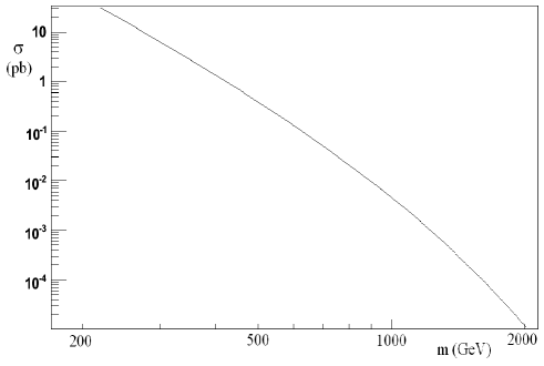
Figure 3: Cross section of the process $pp\to\tilde{t}\tilde{t}^{*}$ at the LHC, $\sqrt{s}=14$ TeV, at tree level. Factorization and renormalization scales were set to $\mu=M_{\tilde{t}}$, and the CTEQ6L1 parton distribution function set [27] was used.

Stop pair production cross section at the LHC, computed using the MadGraph/MadEvent v4 software package [26], is shown in Fig. 3. At the benchmark point, we find $\sigma(pp\to\tilde{t}_{2}\tilde{t}_{2}^{*})=0.05$ pb, corresponding to about 500 $\tilde{t}_{2}$ pairs per year at the initial design luminosity of 10 fb^-1/year. The produced $\tilde{t}_{2}$ decays promptly, with branching ratios listed in Table 3; in about 52% of the events, either one or both of the produced stops decays in the $\tilde{t}_{1}Z$ mode. This decay is followed by a cascade

$$\tilde{t}_{1}\to\chi_{1}^{+}b,~{}~{}~{}\chi_{1}^{+} \to u\bar{d}\chi_{1}^{0}~{}/~{}c\bar{s}\chi_{1}^{0},$$ (23)

$$\to \ell^{+}\nu\chi_{1}^{0},$$

where the jets and leptons produced in the $\chi_{1}^{+}$ decays are very soft due to a small chargino-neutralino mass splitting. The details of this cascade are particular to the chosen BP, and are quite model-dependent. There are, however, two model-independent features true for all $\tilde{t}_{2}$ and $\tilde{t}_{1}$ decays: the cascade always contains a $b$ jet (produced either directly or via top decay), and it always ends with the lightest supersymmetric particle (LSP), the neutralino $\chi_{1}^{0}$, giving a missing transverse energy signature. In order to make the analysis as model-independent as possible, we focus on an inclusive signature,

$$Z(\ell^{+},\ell^{-})+2j_{b}+\mbox{$E{\!\!\!\!}/_{T}$}+X,$$ (24)

where $Z(\ell^{+},\ell^{-})$ denotes a lepton pair ($\ell=e$ or $\mu$) with the invariant mass at the $Z$ peak. The presence of energetic leptons ensures that essentially all such events will be triggered on; we will assume a triggering probability of 1 for this analysis. Note that events with hadronic $Z$ decays may in principle be triggered on due to large $E{\!\!\!\!}/_{T}$; however, this sample would suffer from a severe background of purely QCD events with apparent $E{\!\!\!\!}/_{T}$ due to jet energy mismeasurement, and it will not be used in our study. Note also that the requirement that both jets be $b$-tagged can be relaxed, as will be discussed below. While a cleaner sample is obtained if two $b$-tags are required, this sample is smaller due to the less-than-perfect tagging efficiency, which may be relevant since the signal rates are not large.

To assess the observability of the signature (24), we have simulated a statistically significant event sample for the signal and several SM background channels using the MadGraph/ MadEvent v4 software package [26]. This tool package allows us to generate both SM and MSSM processes, so that the signal and backgrounds can be treated uniformly. The parton level events generated by MadEvent were recorded in the format consistent with the Les Houches accord [28, 29]. These events were then passed on to the Pythia package [30], which was used to simulate showering and hadronization, as well as the decays of unstable particles. Finally, the Pythia output was processed by the PGS 3.9 package [31], which provides a simple and realistic simulation of the response of a “typical” particle detector. (A more detailed analysis of the detector effects using complete ATLAS and CMS detector simulation packages would clearly be interesting, but is outside the scope of this study.) The final output was analyzed with ROOT, using only detector level information for event reconstruction.

The following SM backgrounds have been considered in detail:

• $jjZZ$, which can produce the signature (24) if one $Z$ decays invisibly and the other one is reconstructed in $\ell^{+}\ell^{-}$;

• $t\bar{t}Z$, with $Z\to\ell^{+}\ell^{-}$ and one or both tops decaying leptonically (with $E{\!\!\!\!}/_{T}$ due to neutrinos), or both tops decaying hadronically (with $E{\!\!\!\!}/_{T}$ due to jet energy mismeasurement).

• $t\bar{t}$, with both tops decaying leptonically and the invariant mass of the two leptons accidentally close to $m_{Z}$.

The total production cross sections (with $p_{T,{\rm jet}}^{\rm min}=50$ GeV for the $jjZZ$ channel) and the size of the event sample used in our analysis for each channel are listed in the first two rows of Table 4. To identify the events matching the signature (24), we impose the following set of requirements on the event sample:

1. Two opposite-charge same-flavor leptons must be present with $\sqrt{s(\ell^{+}\ell^{-})}=M_{Z}\pm 2$ GeV.

2. Two hard jets must be present, with $p_{T}>125$ GeV for the first jet and $p_{T}>50$ GeV for the second jet;

3. At least one of the two highest-$p_{T}$ jets must be $b$-tagged;

4. The boost factor of the $Z$ boson, $\gamma(Z)=1/\sqrt{1-v_{Z}^{2}}$, reconstructed from the lepton pair, must be larger than 2.0;

5. A missing $E_{T}$ cut, $\mbox{$E{\!\!\!\!}/_{T}$}>225$ GeV.

	signal: $\tilde{t}_{2}\tilde{t}_{2}^{*}$	$jjZZ$	$t\bar{t}Z$	$t\bar{t}$	$jjZ$
$\sigma_{\rm prod}$(pb)	0.051	0.888	0.616	552	824
total simulated	9964	159672	119395	3745930	1397940
1. leptonic $Z$(s)	1.4	4.5	2.6	0.04	2.1
2(a). $p_{t}(j_{1})>125$ GeV	89	67	55	21	41
2(b). $p_{t}(j_{2})>50$ GeV	94	93	92	76	84
3. $b$-tag	64	8	44	57	5
4. $\gamma(Z)>2.0$	89	66	69	26	68
5. $\mbox{$E{\!\!\!\!}/_{T}$}>225$ GeV	48	2.2	4.4	1.7	$<0.9$ (95% c.l.)
					0 (ext.)
$N_{\rm exp}$(100 $fb^{-1}$)	16.4	2.8	10.8	8.8	$<177$ (95% c.l.)
					0 (ext.)

Table 4: Summary of the analysis of observability of the supersymmetric golden region signature (24). First row: Production cross section for the signal and background processes at the LHC. Second row: Number of Monte Carlo events used in the analysis. Rows 3–8: Cut efficiencies, in%. Last row: The expected number of events for an integrated luminosity of 100 fb^-1.

The efficiencies of these cuts are given in Table 4, and the $E{\!\!\!\!}/_{T}$ distribution of the events passing cuts 1–4 is shown in Figure 4. While the overall rate of the SM background processes is much higher than the signal rate, the cuts 1-5 are quite effective in discriminating signal from background. Assuming that the search is statistics-limited, we estimate that a 3-sigma observation would require 75 fb^-1 of data, while a definitive 5-sigma discovery is possible with 210 fb^-1. Note that one important contribution to the background, from the $t\bar{t}$ channel, can be effectively measured from data by measuring the event rates with dilepton invariant masses away from the $Z$ peak and performing shoulder subtraction. This procedure is likely to be statistics-limited. However, systematic uncertainties in other background contributions could play a role in limiting the reach, and should be studied carefully with a more detailed detector simulation.

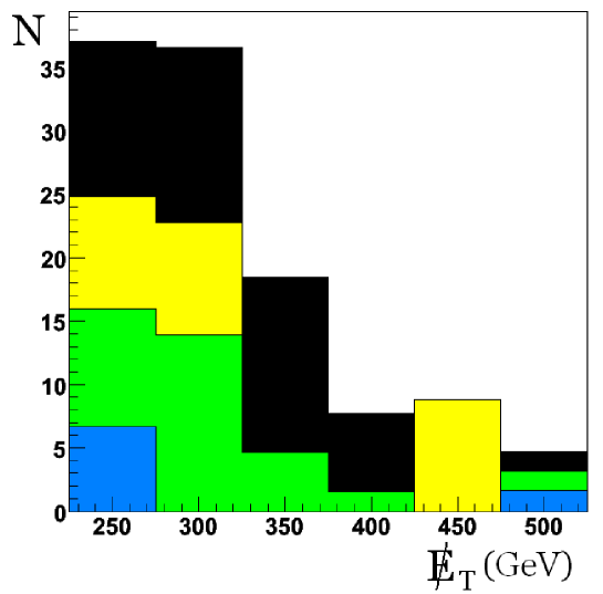
Figure 4: Missing $E_{T}$ distribution of the events passing cuts 1–4. Signal is shown in black; $jjZZ$, $t\bar{t}Z$ and $t\bar{t}$ backgrounds are shown in blue/dark-gray, green/gray, and yellow/light-gray, respectively. The normalization corresponds to an integrated luminosity of 300 fb^-1 at the LHC.

We also briefly considered several other irreducible SM backgrounds which are expected to be less significant than the ones listed in Table 4, but might nevertheless be relevant. The most important one of these is $t\bar{t}j$, where $j$ is a hard jet. The cross section for this channel is suppressed compared to $t\bar{t}$, but the presence of the additional hard jet increases the probability that the events will pass the jet $p_{T}$ cut (cut 2). We find a parton-level cross section $\sigma(t\bar{t}j,p_{T}^{j}>125~{}{\rm GeV})=65$ pb. Assuming conservatively that all these events pass the cut 2, and that the efficiencies of all other cuts are the same as for the $t\bar{t}$ sample, we expect that this background would add at most about 50% to the $t\bar{t}$ rate. As in the $t\bar{t}$ case, this contribution can be subtracted using data away from the $Z$ peak in the lepton invariant mass distribution. Assuming that the statistical error dominates this subtraction, the net effect would be an increase in the integrated luminosity required to achieve the same level of significance by at most about 10%. Other backgrounds we considered are three vector boson channels $ZZZ$, $ZZW$, and $ZWW$; as well as channels with single top production, $tZj$ and $\bar{t}Zj$. Combining the parton-level cross sections for these channels with the branching ratios of decays producing the signature (24) results in event rates that are too small to affect the search.

While the SM processes considered above genuinely produce the signature (24), other SM processes may contribute to the background due to detector imperfections. We expect that the dominant among these is the process $jjZ$, with $Z\to\ell^{+}\ell^{-}$ and apparent $E{\!\!\!\!}/_{T}$ due to jet energy mismeasurement or other instrumental issues. We conducted a preliminary investigation of this background by generating and analyzing a sample of $1.4\times 10^{6}$ $jjZ$ events with $p_{T,{\rm jet}}^{\rm min}=50$ GeV (see the last column of Table 4). None of the events in this sample pass the cuts 1-5. This allows us to put a 95% c.l. bound on the combined efficiency of this set of cuts for the $jjZ$ sample of about $2\times 10^{-6}$, corresponding to a background rate about 10 times larger than the signal rate. However, we expect that the actual $jjZ$ background rate is well below this bound, since all 349 events in our sample that pass the cuts 1–4 in fact have $E{\!\!\!\!}/_{T}$ below 50 GeV. We find that the $E{\!\!\!\!}/_{T}$ distribution of these 349 events can be fit with an exponential, $N\propto e^{-0.10\mbox{$E{\!\!\!\!}/_{T}$}}$, where $E{\!\!\!\!}/_{T}$ is in units of GeV. Assuming that this scaling adequately describes the tail of the distribution at large $E{\!\!\!\!}/_{T}$, we estimate that the rate of $jjZ$ events passing all 5 cuts is completely negligible and that this background should not present a problem. This conclusion is of course rather preliminary, and this issue should be revisited once the performance of the LHC detectors is understood using real data. Note that the necessity to understand the shape and normalization of the large apparent $E{\!\!\!\!}/_{T}$ tail from SM processes with large cross sections is not unique to the signature discussed here, but is in fact crucial for most SUSY searches at the LHC.

	signal: $\tilde{t}_{2}\tilde{t}_{2}^{*}$	$jjZZ$	$t\bar{t}Z$	$t\bar{t}$	$jjZ$
$\sigma_{\rm prod}$(pb)	0.051	0.888	0.616	552	824
total simulated	9964	159672	119395	3745930	1397940
1. leptonic $Z$(s)	1.4	4.5	2.6	0.04	2.1
2(a). $p_{t}(j_{1})>125$ GeV	89	67	55	21	41
2(b). $p_{t}(j_{2})>50$ GeV	94	93	92	76	84
3. 2 $b$-tags	22	0.4	6	9	0.3
4. $\mbox{$E{\!\!\!\!}/_{T}$}>225$ GeV	56	$<2$	$<5$	$<3$	$<10$ (95% c.l.)
$N_{\rm exp}$(100 $fb^{-1}$)	7	$<2.4$	$<2.7$	$<8.8$	$<177$ (95% c.l.)

Table 5: Same as Table 4, with an alternative set of requirements including 2 $b$-tagged jets.

As an alternative, we considered a variation of the analysis where the cuts 1, 2, and 5 are unchanged, cut 4 is eliminated, and two $b$-tagged jets are required. The cut efficiencies for this analysis are summarized in Table 5. Unfortunately, the Monte Carlo samples used in our analysis are not large enough to reliably estimate the efficiencies of this set of cuts applied to the backgrounds, since only one event out of all background samples passes the cuts. Therefore we list the 95% c.l. upper bounds on the efficiencies, and on the number of background events expected for a 100 fb^-1 event sample, in the table. It is clear that while the second $b$-tag is quite efficient in improving the S/B ratio, this search suffers from low statistics, with only 7 signal events expected in a 100 fb^-1 data sample.

To summarize, our analysis indicates that, for the MSSM parameters at the benchmark point, the signature (24) of the split-stop spectrum can be discovered at the LHC. The chosen BP is typical of the golden region, and this conclusion should generally hold as the MSSM parameters are varied away from the BP, scanning this region. There are, however, several exceptional parts of the parameter space where the observability of this signature could be substantially degraded. These include:

• Large $\tilde{m}_{2}$ region: The $\tilde{t}_{2}$ production cross section drops rapidly with its mass, see Fig. 3, suppressing the signal rates;

• Small $\theta_{t}$ region: While non-zero $\theta_{t}$ is required in the golden region, values as small as $\theta_{t}=\pi/15$ are allowed (see Fig. 2). The branching ratio Br($\tilde{t}_{2}\to Z\tilde{t}_{1}$) is proportional to $\sin^{2}2\theta_{t}$, see Eq. (21), and the event rate is suppressed at small $\theta_{t}$;

• Small $\tilde{t}_{1}$-LSP mass difference: The absence of hard jets in this case would make the signal/background discrimination more difficult.

In these special regions, observing the signature (24) may not be feasible at the LHC. These limitations should be kept in mind when theoretical interpretation of a search for the signature (24) is given.

5 Alternative Interpretations of the $Z+2j_{b}+\mbox{$E{\!\!\!\!}/_{T}$}+X$ Signature

Unfortunately, observing an excess of events in the channel (24) at the LHC does not prove that the decay $\tilde{t}_{2}\to\tilde{t}_{1}Z$ is occuring. Even within the MSSM, this is not the only possible interpretation of such an excess. The simplest alternative interpretation is stop or sbottom production, followed by a cascade decay containing a $b$ quark and a $Z$ boson from a neutralino or chargino decay: $\chi^{0}_{j}\to\chi_{i}^{0}Z$ (due to the higgsino components of the neutralinos) or $\chi^{\pm}_{2}\to\chi^{\pm}_{1}Z$. Can this alternative interpretation be ruled out based on data?

One useful input for discriminating between these two interpretations is whether a signal is observed in a search identical to the one presented in Section 4, but requiring that the jets not be $b$-tagged. If the signal is due to $\tilde{t}_{2}\to\tilde{t}_{1}Z$, all signal events contain energetic $b$ quarks, and the number of events in this search would be zero if $b$ tagging were perfect. The actual number of expected events under realistic conditions can be deduced from the error rate in $b$ tagging, which can be measured elsewhere. If the signal is due to $\chi^{0}_{j}\to\chi_{i}^{0}Z$ or $\chi^{\pm}_{2}\to\chi^{\pm}_{1}Z$, it does not have to be associated preferentially with third-generation squark production, and the number of events without $b$ tags could be substantially larger than this expectation. This argument could be used to rule out the $\tilde{t}_{2}\to\tilde{t}_{1}Z$ interpretation. Unfortunately, however, it cannot be used to confirm it: the pattern consistent with the $\tilde{t}_{2}\to\tilde{t}_{1}Z$ interpretation may also appear if the events are actually due to chargino or neutralino decays, provided that the first two generations of squarks are substantially heavier than their counterparts of the third generation and their production cross section is suppressed. A direct measurement of the squark masses could break this degeneracy. If the first two generations of squarks were found to be light, but no signal is seen in $Z+2j+\mbox{$E{\!\!\!\!}/_{T}$}$ with non-$b$ jets, the “split stop” interpretation of the signal (24) would be preferred.

Figure 5: Cascade decays in the MSSM leading to the $Z+2j+\mbox{$E{\!\!\!\!}/_{T}$}$ signature: (a) the chain characteristic of the golden region; (b) an alternative chain.

A more direct way to discriminate between the two interpretations would be to study the distribution of the events as a function of the $Z$-jet invariant mass $s_{jZ}\equiv(p_{j}+p_{Z})^{2}$. This strategy is the same as the recently proposed method of discriminating between SUSY and alternative theories with same-spin “superpartners” [32, 33], but in this case it is applied to distinguishing two processes within the MSSM. Consider the Feynman diagrams corresponding to the two interpretations of the signal, shown in Figure 5. In the case of $\tilde{t}_{2}\to\tilde{t}_{1}Z$ decays, the $Z$ and the jet are separated by a scalar (stop) line, and their directions are uncorrelated. In the case of chargino or neutralino decays, the $Z$ and the jet are separated by a fermion line, and spin correlations between their directions are possible. Unfortunately, in the neutralino case, no such correlations occur, because of the non-chiral nature of the $\chi^{0}_{i}\chi^{0}_{j}Z$ coupling [33]. In the chargino case, however, the coupling has the form [1]

$$-\frac{g}{2c_{w}}\,\bar{\tilde{\chi}}_{i}\gamma^{\mu}\,\left[C^{L}_{ij}(1-\gamma_{5})\,+\,C^{R}_{ij}(1+\gamma_{5})\right]\tilde{\chi}_{j}\,,$$ (25)

where

$$C^{L}_{ij} = V_{i1}V_{j1}^{*}+\frac{1}{2}V_{i2}V^{*}_{j2}\,,$$

$$C^{R}_{ij} = U_{i1}^{*}U_{j1}+\frac{1}{2}U_{i2}^{*}U_{j2}\,.$$ (26)

Here, $U$ and $V$ are the rotations of the negatively-charged and positively-charged charginos, respectively, required to diagonalize the chargino mass matrix. Since in general $U\not=V$, the couplings (25) are generically chiral. The stop-bottom-chargino coupling is also generically chiral: it has the form

$$\bar{b}(A^{L}_{ij}P_{R}+A^{R}_{ij}P_{L})\tilde{\chi}^{c}_{i}\tilde{t}_{j},$$ (27)

which can be equivalently rewritten as

$$\bar{\tilde{\chi}}_{i}(A^{L}_{ij}P_{R}+A^{R}_{ij}P_{L})b^{c}\tilde{t}_{j}.$$ (28)

Here

$$A^{L}_{ij} = gV_{i1}R^{t}_{j1}+\frac{y_{t}}{s_{\beta}}V_{i2}R^{t}_{j2}\,,$$

$$A^{R}_{ij} = \frac{y_{b}}{c_{\beta}}U_{i2}R^{t}_{j1}\,,$$ (29)

where $R^{t}$ is the matrix diagonalizing the stop masses: $(\tilde{t}_{1},\tilde{t}_{2})^{T}=R^{t}(\tilde{t}_{L},\tilde{t}_{R})^{T}$. Squaring the matrix element ${\cal M}$ for the decay $\tilde{t}_{j}\to b+Z+\chi^{+}_{1}$, see Fig. 5 (b), and summing over the final-state polarizations yields

$$\sum_{{\rm pol}}|{\cal M}|^{2}\,\propto(|A^{L}_{j2}|^{2}-|A^{R}_{j2}|^{2})\,(|C^{L}_{12}|^{2}-|C^{R}_{12}|^{2})\,s_{bZ}+{\rm const},$$ (30)

where the constant terms do not depend on $s_{bZ}$, narrow-width approximation for $\chi^{\pm}_{2}$ has been used, and the $b$ quark mass was neglected. The charge-conjugate decay $\tilde{t}^{*}_{j}\to\bar{b}+Z+\chi^{-}_{1}$ has the same asymmetry. Observing a linear dependence of the event rate on $s_{bZ}$ would provide clear evidence against the interpretation of the signal in terms of the process in Fig. 5 (a). Of course, in a real experiment, the asymmetry would be partially washed out by combinatoric backgrounds, as well as possible non-chiral decay chains containing the same final state. A detailed analysis of the observability of the correlation in Eq. (30) is beyond the scope of this paper.

While our analysis so far focused on the decay $\tilde{t}_{2}\to\tilde{t}_{1}Z$ as a signature of the MSSM golden region, there are two other, closely related decays that are also characteristic of this region:

$$\tilde{t}_{2}\to\tilde{b}_{L}W^{+},~{}~{}~{}\tilde{b}_{L}\to\tilde{t}_{1}W^{-}.$$ (31)

For example, at the benchmark point used for the analysis in Section 4, these two decays have branching ratios of 15% and 43%, respectively. Stop or sbottom pair-production followed by these decays leads to a signature

$$W+2j_{b}+\mbox{$E{\!\!\!\!}/_{T}$}+X.$$ (32)

This signature is complementary to the $Z+2j_{b}+\mbox{$E{\!\!\!\!}/_{T}$}+X$ signature studied above. On the one hand, it suffers from higher backgrounds, since the $W$ cannot be fully reconstructed in purely leptonic channels. On the other hand, its interpretation within the MSSM is somewhat cleaner. The leading alternative interpretation of the signature (32) is that the $W$’s are produced in chargino $\to$ neutralino decays. But the chargino-neutralino coupling is chiral, and the directions of the $W$ and the associated jet are correlated. If the $W$ is sufficiently boosted, this will result in an observable linear dependence of the cross section on $s_{\ell j}\equiv(p_{\ell}+p_{j})^{2}$, where $\ell$ is the lepton daughter of the $W$ [33]. If, on the other hand, the $W$ is produced in decays of scalars, such as the processes (31), the distribution of events in $s_{\ell j}$ should be flat.

To summarize, even if the MSSM is assumed to be the underlying model, the interpretation of events with vector bosons associated with jets and missing $E_{T}$ is not unambiguous. Careful comparisons of the rates with and without $b$ jets, as well as the distribution of events in vector boson-jet invariant masses, would be required to remove the ambiguity. This may take considerably more data than the discovery of an excess over the SM backgrounds in these channels.

If the MSSM is not assumed from the beginning, the question of interpretation becomes even more confusing. For example, in the Littlest Higgs model with T-parity [34], $Z$ bosons can be produced in the decay $W^{3}_{H}\to ZB_{H}$, due to the mixing between the $SU(2)$ and $U(1)$ heavy gauge bosons. A similar decay involving the Kaluza-Klein states of the $SU(2)\times U(1)$ gauge bosons can occur in models with universal extra dimensions (UED) [35]. Again, a careful study of spin correlations would be necessary to disentangle these possibilities. Understanding the nature of such correlations in various models is an interesting direction for future work.

6 Conclusions

In this paper, we discussed an LHC signature of the MSSM characteristic of the “golden region” in the model parameter space. The advantage of this signature is that it directly probes the features of the stop spectrum that are dictated by naturalness and the Higgs mass bound. Experimentally, the signature is not straightforward, but the results of our simulations indicate that it should be within reach at the LHC.

Given the strong theoretical motivation for the signature discussed here, we encourage experimental collaborations to perform a more detailed study of its observability. The analysis of this paper relied on a set of simple rectangular cuts, and no systematic procedure to optimize the cuts was employed. It is very likely that a better algorithm for signal/background discrimination, perhaps using modern data analysis tools such as neural networks or decision trees, would significantly enhance the reach. On the other hand, it should be noted that we ignored systematic uncertainties on the background rates in our reach estimates, and that no fully realistic detector simulation was attempted.

If the first round of the LHC results points towards an MSSM-like theory, obtaining experimental information about the stop spectrum, and in particular testing whether the “golden region MSSM” hypothesis is correct, will become an important priority for the LHC experiments. An indirect way to shed some light on this issue by identifying the stop loop contributions to the Higgs production cross section and mass has been recently proposed by Dermisek and Low [36]. This is complementary to the direct probe explored in this paper. It would be interesting to explore other experimental consequences of the golden region hypothesis.

Acknowledgments

Giacomo Cacciapaglia has collaborated with us at the early stages of this project. We gratefully acknowledge his contributions to our understanding of the implications of naturalness and experimental data on the MSSM parameters. We are grateful to Patrick Meade and Michael Peskin for useful discussions. This research is supported by the NSF grant PHY-0355005.

References

- [1] H. E. Haber and G. L. Kane, Phys. Rept. 117 (1985) 75.
- [2] S. P. Martin, arXiv:hep-ph/9709356.
- [3] R. Barbieri and A. Strumia, arXiv:hep-ph/0007265.
- [4] See, for example, P. Batra, A. Delgado, D. E. Kaplan and T. M. P. Tait, JHEP 0402, 043 (2004) [arXiv:hep-ph/0309149]; R. Harnik, G. D. Kribs, D. T. Larson and H. Murayama, Phys. Rev. D 70, 015002 (2004) [arXiv:hep-ph/0311349]; R. Dermisek and J. F. Gunion, Phys. Rev. Lett. 95, 041801 (2005) [arXiv:hep-ph/0502105]; T. Roy and M. Schmaltz, JHEP 0601, 149 (2006) [arXiv:hep-ph/0509357]; C. Csaki, G. Marandella, Y. Shirman and A. Strumia, Phys. Rev. D 73, 035006 (2006) [arXiv:hep-ph/0510294]; G. Burdman, Z. Chacko, H. S. Goh and R. Harnik, arXiv:hep-ph/0609152.
- [5] G. F. Giudice and R. Rattazzi, arXiv:hep-ph/0606105.
- [6] K. Choi, K. S. Jeong, T. Kobayashi and K. i. Okumura, Phys. Lett. B 633, 355 (2006) [arXiv:hep-ph/0508029]; R. Kitano and Y. Nomura, Phys. Lett. B 631, 58 (2005) [arXiv:hep-ph/0509039].
- [7] K. Choi, K. S. Jeong and K. i. Okumura, JHEP 0509, 039 (2005) [arXiv:hep-ph/0504037].
- [8] A. Pierce and J. Thaler, JHEP 0609, 017 (2006) [arXiv:hep-ph/0604192].
- [9] K. Choi, K. S. Jeong, T. Kobayashi and K. i. Okumura, arXiv:hep-ph/0612258.
- [10] R. Dermisek and H. D. Kim, Phys. Rev. Lett. 96, 211803 (2006) [arXiv:hep-ph/0601036]; R. Dermisek, H. D. Kim and I. W. Kim, JHEP 0610, 001 (2006) [arXiv:hep-ph/0607169].
- [11] R. Kitano and Y. Nomura, Phys. Rev. D 73, 095004 (2006) [arXiv:hep-ph/0602096].
- [12] H. Baer, X. Tata and J. Woodside, Phys. Rev. D 42, 1450 (1990); H. Baer, C. Balazs, A. Belyaev, T. Krupovnickas and X. Tata, JHEP 0306, 054 (2003) [arXiv:hep-ph/0304303].
- [13] R. Barbieri and G. F. Giudice, Nucl. Phys. B 306, 63 (1988).
- [14] S. Schael et al. [ALEPH Collaboration], Eur. Phys. J. C 47, 547 (2006) [arXiv:hep-ex/0602042].
- [15] W. M. Yao et al. [Particle Data Group], J. Phys. G 33, 1 (2006).
- [16] G. Degrassi, S. Heinemeyer, W. Hollik, P. Slavich and G. Weiglein, Eur. Phys. J. C 28, 133 (2003) [arXiv:hep-ph/0212020].
-
[17]
The FeynHiggs package can be downloaded from
http://wwwth.mppmu.mpg.de/members/heinemey/feynhiggs/index.html
For a recent discussion, see M. Frank et. al., arXiv:hep-ph/0611326. See also Ref. [16]; S. Heinemeyer, W. Hollik and G. Weiglein, Eur. Phys. J. C 9, 343 (1999) [arXiv:hep-ph/9812472]; Comput. Phys. Commun. 124, 76 (2000) [arXiv:hep-ph/9812320]. -
[18]
The SuSpect package can be downloaded from
http://www.lpta.univ-montp2.fr/users/kneur/Suspect/
and is discussed in A. Djouadi, J. L. Kneur and G. Moultaka, arXiv:hep-ph/0211331. - [19] M. Carena, J. R. Espinosa, M. Quiros and C. E. M. Wagner, Phys. Lett. B 355, 209 (1995) [arXiv:hep-ph/9504316].
- [20] E. Brubaker et al. [Tevatron Electroweak Working Group], arXiv:hep-ex/0608032.
- [21] A. Djouadi, P. Gambino, S. Heinemeyer, W. Hollik, C. Junger and G. Weiglein, Phys. Rev. D 57, 4179 (1998) [arXiv:hep-ph/9710438].
- [22] S. Chen et al. [CLEO Collaboration], Phys. Rev. Lett. 87, 251807 (2001) [arXiv:hep-ex/0108032]; B. Aubert et al. [BaBar Collaboration], arXiv:hep-ex/0507001; P. Koppenburg et al. [Belle Collaboration], Phys. Rev. Lett. 93, 061803 (2004) [arXiv:hep-ex/0403004]; E. Barberio et al. [Heavy Flavor Averaging Group (HFAG)], arXiv:hep-ex/0603003.
- [23] G. W. Bennett et al. [Muon g-2 Collaboration], Phys. Rev. Lett. 92, 161802 (2004) [arXiv:hep-ex/0401008].
- [24] R. Barbieri and G. F. Giudice, Phys. Lett. B 309, 86 (1993) [arXiv:hep-ph/9303270].
-
[25]
The SDECAY package can be downloaded from
http://lappweb.in2p3.fr/~muehlleitner/SDECAY/
and is discussed in M. Muhlleitner, A. Djouadi and Y. Mambrini, Comput. Phys. Commun. 168, 46 (2005) [arXiv:hep-ph/0311167]. -
[26]
MadGraph/MadEvent v4 can be downloaded from
http://madgraph.phys.ucl.ac.be/
For a discussion of the Madgraph project, see F. Maltoni and T. Stelzer, JHEP 0302, 027 (2003). [arXiv:hep-ph/0208156]. - [27] J. Pumplin et. al. JHEP 0207, 012 (2002) [arXiv:hep-ph/0201195].
- [28] E. Boos et al., arXiv:hep-ph/0109068.
- [29] P. Skands et al., JHEP 0407, 036 (2004) [arXiv:hep-ph/0311123].
- [30] T. Sjöstrand et al., Comput. Phys. Commun. 135, 238 (2001). [arXiv:hep-ph/0010017]; T. Sjostrand, S. Mrenna and P. Skands, JHEP 0605, 026 (2006) [arXiv:hep-ph/0603175].
-
[31]
The PGS detector simulation package can be downloaded from
http://www.physics.ucdavis.edu/~conway/research/software/pgs/pgs.html
or, as a part of the LHC Olympics black box generation software package, from http://www.jthaler.net/olympics/blackbox.tgz - [32] A. J. Barr, Phys. Lett. B 596, 205 (2004) [arXiv:hep-ph/0405052]; J. M. Smillie and B. R. Webber, JHEP 0510, 069 (2005) [arXiv:hep-ph/0507170].
- [33] L. T. Wang and I. Yavin, arXiv:hep-ph/0605296.
- [34] I. Low, JHEP 0410, 067 (2004) [arXiv:hep-ph/0409025]; J. Hubisz and P. Meade, Phys. Rev. D 71, 035016 (2005) [arXiv:hep-ph/0411264]; J. Hubisz, P. Meade, A. Noble and M. Perelstein, JHEP 0601, 135 (2006) [arXiv:hep-ph/0506042]. For a pedagogical introduction, see M. Perelstein, Prog. Part. Nucl. Phys. 58, 247 (2007) [arXiv:hep-ph/0512128].
- [35] T. Appelquist, H. C. Cheng and B. A. Dobrescu, Phys. Rev. D 64, 035002 (2001) [arXiv:hep-ph/0012100]; H. C. Cheng, K. T. Matchev and M. Schmaltz, Phys. Rev. D 66, 056006 (2002) [arXiv:hep-ph/0205314].
- [36] R. Dermisek and I. Low, arXiv:hep-ph/0701235.