Anomalous diffusion of pions at RHIC

Abstract

After pointing out the difference between normal and anomalous diffusion, we consider a hadron resonance cascade (HRC) model simulation for particle emission at RHIC and point out that rescattering in an expanding hadron resonance gas leads to a heavy tail in the source distribution. The results are compared to recent PHENIX measurements of the tail of the particle emitting source in Au+Au collisions at RHIC. In this context, we show how can one distinguish experimentally the anomalous diffusion of hadrons from a second order QCD phase transition.

“ It does not make any difference
how beautiful your guess is.
It does not make any difference
how smart you are,
who made the guess, or what his name is -
if it disagrees with experiment, it is wrong.”
                 
                                    /R.P. Feynman/

I INTRODUCTION

Various new techniques are being developed in a vibrant and inspiring, sometimes challenging and puzzling sub-field, named recently by Lednicky Lednicky:2005af as correlation femtoscopy. A series of inspiring and stimulating recent reviews Padula:2004ba ; Csorgo:2005gd ; Lisa:2005dd ; Lisa:2005js ; Hwa:2007rp re-connected femtoscopy to the search of new phases of QCD as well as other new, sometimes unexpected, sometimes puzzling expectations and observations. One of these new experimental results has been a recent PHENIX measurement of source images in Au+Au collisions at $\sqrt{s_{NN}}=200$ GeV that found evidence for a non-Gaussian structure and a heavy (larger than Gaussian) tail in the source distribution for pions  PHENIX-imaging . This points to an interesting new direction, going beyond investigating only the means and the variances of the source distributions on the scales of femtometers.

Resonance decays are known to be able to produce long, non-Gaussian tails, because some of the resonances have large decay times as compared to the characteristic 4-5 fm/c source sizes extracted from interferometric measurements in Au+Au collisions at RHIC. In fact, a smaller and smaller fraction of resonances have larger and larger life-times, and this effect was considered first by Białas Bialas:1992ca who argued that even a cut power-law correlation functions may appear, due to the fact that the decay times of pion producing resonances have a broad probability distribution. Another possible conventional source for such a heavy tail of the source of pions might be the elastic rescattering of the produced hadrons: as the hadron gas expands, the system becomes cooler and more and more diluted, hence the mean free path becomes larger and larger. In many hydrodynamical calculations, an idealized freeze-out process is assumed, when the mean free path suddenly jumps from 0 (the hydrodynamic limit) to infinity (the freeze-out limit). More realistically, the mean free path diverges to infinity in a finite time interval, and rescattering in a time dependent mean free path system is known to lead to new phenomena, which has been studied in great detail under the name of anomalous diffusion in other branches of physics. One of the experimentally observed characteristics of such an anomalous diffusion pattern was the appearance of approximately power-law shaped tails in the coordinate space distributions, which is to be contrasted to the Gaussian, strongly decaying tails observed in normal diffusion or in Brownian motion. We shall explore the phenomena of anomalous diffusion in the context of heavy ion physics, first pointing out its general mathematical properties and its relations to Lévy source distributions, following the review of Klafter and Metzler on anomalous diffusion MK-rep . Then we shall explore anomalous diffusion of pions, kaons and protons in Au+Au collisions at $\sqrt{s_{NN}}=200$ GeV colliding energies using the simplest possible tool, namely the conventional Hadronic Resonance Cascade (HRC) model of Tom Humanic Humanic:2005ye . First we compare the results of this HRC simulation with PHENIX data. Then we investigate the sensitivity of the characteristics of the simulation for various experimentally available controls, like the selection of the centrality class of the events or the selection of a transverse momentum region of the pair. Finally we summarize and conclude. As a starting point, let us consider a simplified version of the presentation in ref. MK-rep , to review the equations of normal and anomalous diffusions in the same framework, based on a master equation approach.

II Normal Diffusion

Normal diffusion corresponds to a physical process when one investigates the motion of a test particle in a medium, which has some grid like structure with fixed (say, $\Delta x$) lattice constant, (equidistant cells) and jumps (of a fixed frequency) are allowed to nearest neighboring cells. Let us for simplicity consider a one dimensional, normal diffusion process in the framework of master equation approach. The time is denoted by $t$. A test particle is initially located at a given cell, denoted by $j=0$. Different cells are indexed by the integer $j\in\mathbb{Z}$. The probability distribution of finding the particle in cell $j$ at time $t$ is denoted by $W_{j}(t)$. (Note that $W_{j}(t)$ can be considered as analogous to the particle emission function $S(x,t)$, that we frequently encounter in particle interferometry and femtoscopy.) Suppose that particles may jump from the given cell to its nearest neighbors, randomly up and down, at certain regular but small time intervals $\Delta t$. The continuum limit means $\Delta t\rightarrow 0$, $\Delta x\rightarrow 0$ in such a way that the mean free path (and also the mean collision time) remains constant.

In this situation, the following master equation drives the time evolution in this material:

$$W_{j}(t+\Delta t)=\frac{1}{2}W_{j-1}(t)+\frac{1}{2}W_{j+1}(t).$$ (1)

We rewrite this discretized form to a continuous form by introducing the continuous coordinate variable $x$. We assume that the $\Delta x$ step size is infinitesimally small compared to the overall length-scale of the medium, and that the time interval between the subsequent jumps is small as compared to the time duration corresponding to the observation of the diffusion process. These assumptions yield the following leading order Taylor expansions:

$$W_{j}(t+\Delta t)=W_{j}(t)+\Delta t\frac{\partial W_{j}}{\partial t}+{\cal O}(\Delta t^{2}),$$ (2)

$$W_{j\pm 1}(t)=W(x,t)\pm\Delta x\frac{\partial W}{\partial x}+\frac{(\Delta x)^{2}}{2}\frac{\partial^{2}W}{\partial x^{2}}+{\cal O}(\Delta x^{3}),$$ (3)

and these expressions can be combined to derive the continuum form of the diffusion equation

$$\frac{\partial W}{\partial t}=K_{1}\frac{\partial^{2}}{\partial x^{2}}W(x,t).$$ (4)

All properties of this matter are characterized by the diffusion constant $K_{1}=\lim_{\Delta x\rightarrow 0,\Delta t\rightarrow 0}\frac{\Delta x^{2}}{2\Delta t}$, which corresponds to the mean squared displacement per unit time.

The above (normal) diffusion equation can be solved easily by introducing the Fourier-transform

$$W(k,t)=\int\,dx\exp(ikx)W(x,t),$$ (5)

that leads to the momentum-space diffusion equation

$$\frac{\partial W}{\partial t}=-K_{1}k^{2}W(k,t).$$ (6)

The solution of this equation is a Gaussian function of $k$ that can be converted back to the coordinate-space distribution to yield the solution of the normal diffusion equation:

$$W(x,t)=\frac{1}{\sqrt{4\pi K_{1}t}}\exp\left(-\frac{x^{2}}{4K_{1}t}\right),$$ (7)

corresponding to normal or Gaussian diffusion of test particles. The initial condition corresponding to this solution is indeed

$$W_{0}(x)\equiv\lim_{t\rightarrow 0}W(x,t)=\delta(x)\,,$$ (8)

corresponding to a localized package inserted in a material with homogeneous, time independent properties. Hence in a homogeneous and time independent medium, the diffusion of point-like initial source yields a Gaussian source density distribution, and the mean square of this Gaussian, $R^{2}=2K_{1}t$ increases linearly with increasing time. This behavior will be contrasted to the more general case, when both the jump lengths and the jump frequencies have a continuous probability distribution.

III Anomalous Diffusion

We again follow Metzler and Klafter in deriving anomalous diffusion from the so-called continuous time random walk models. Suppose that the jump length and jump time have the probability distribution $\psi(x,t)$. Then the jump length distribution $\lambda(x)$ and the waiting time or jump time distribution $w(t)$ reads as

$$\lambda(x) = \int_{0}^{\infty}\psi(x,t)\,\mathrm{d}t,$$ (9)

$$w(t) = \int_{-\infty}^{\infty}\psi(x,t)\,\mathrm{d}x.$$ (10)

Suppose that an external force $F(x)$ also influences the motion of the test particles. These considerations lead to the generalized or anomalous diffusion equation, which is a kind of a generalized Fokker-Planck equation for the phase-space distribution, $W(x,v,t)$:

$$\frac{\partial W}{\partial t}+v\frac{\partial W}{\partial x}+\frac{F(x)}{m}\frac{\partial W}{\partial v}=\eta_{\alpha^{\prime}}{}_{0}D_{t}^{1-\alpha^{\prime}}L_{FP}W,$$ (11)

which contains fractional derivatives and other subtleties that go well beyond the scope of this presentation. For the detailed definition and explanation of this fractional Fokker-Planck equation we refer to  MK-rep . What is important, however, that if the waiting time distribution has a Poissonian shape, the exact solution of this fractional Fokker-Planck equation has a simple form in the momentum space representation:

$$W(k,t)=\exp(-tK^{\alpha}|k|^{\alpha}).$$ (12)

This form is the well known characteristic function (Fourier-transform) of Lévy stable source distributions zol2 ; zol1 ; nolan-chap1 ; nolan-book . Here the parameter $\alpha$ stands for the Lévy index of stability, in general $0<\alpha\leq 2$ for Lévy stable source distributions, and parameter $K$ is an anomalous diffusion constant, $K=\lim_{\Delta x\rightarrow 0,\Delta t\rightarrow 0}\frac{\Delta x^{2}}{2\Delta t^{2/\alpha}}$.

Note that Lévy stable distributions were introduced to particle interferometry studies recently in ref. csorgo-hegyi-zajc , based on general, mathematical arguments like generalized central limit theorems. Anomalous diffusion is a specific example of a physical process that under certain conditions detailed in MK-rep satisfies such generalized central limit theorems: one more rescattering in the diffusion process does not change the limiting behavior of the source distribution.

IV Lévy stable laws and anomalous diffusion

The edification from the previous section is that rescattering in a system with a time dependent mean free path under certain conditions (e.g. Poissonian waiting time distributions) leads to a random Lévy walk (or anomalous diffusion), instead of Brownian motion (or normal, Gaussian diffusion). In case of anomalous diffusion or Lévy walks, the scale parameter grows with time as $R^{\alpha}\propto t$, in contrast to normal diffusion, that corresponds to the $\alpha=2$, $R^{2}\propto t$ special case.

The difference between normal and anomalous diffusion is illustrated in Fig. 1, reproduced from ref. MK-rep .

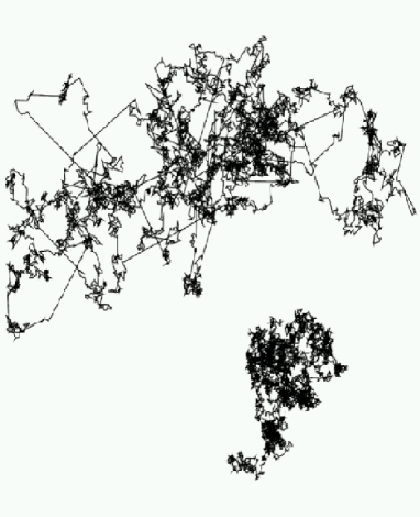
Figure 1: Simple illustration of the qualitative properties of normal diffusion (bottom) and anomalous diffusion (top). In the latter case, large jumps separate various more local parts of the trajectory. The size of the covered region is larger in case of the anomalous diffusion than in case of the Gaussian, normal diffusion. From ref. MK-rep .

Although the mean displacement or the variance of these distributions might diverge, one additional step in the anomalous diffusion does not change the limiting behavior of the process.

It is also interesting to note that the tail of anomalous diffusions has a power-law structure in coordinate space, $S(r)\propto r^{-(d+\alpha)}$ for $r\gg R$, where $d$ is the number of spatial dimensions ($d=3$ in our world), and $\alpha$ is the same Lévy index of stability as before. This asymptotics is yet another important property of the Lévy stable source distributions.

Nature often violates Gaussian universality, mirrored in experimental results which do not follow Gaussian predictions MK-rep . The evidence for a non-Gaussian behavior in multivariate and univariate source distributions has been observed recently also in high energy heavy ion collisions. In fact, the first observation of a non-Gaussian correlation function in Au+Au collisions at RHIC has been made by the STAR collaboration that utilized an Edgeworth expansion STAR-edge and quantified the deviation from the Gaussian structure of the particle emitting source in terms of non-vanishing fourth order cumulant moments of the squared Fourier-transformed source distribution. More recently, the PHENIX Collaboration has applied the imaging method of Brown and Danielewicz imaging to reconstruct the two-particle relative coordinate distribution PHENIX-imaging . In this paper, PHENIX observed a clear deviation from a Gaussian structure, and pointed to the appearance of a heavy tail in the two-particle relative coordinate distribution. In the subsequent part of this manuscript, we investigate if these PHENIX source function data can be reproduced with the help of Monte-Carlo models that incorporate the concept of anomalous diffusion and that are able to describe the more standard observable like single particle spectra and the three dimensional Gaussian fit parameters, $R_{\mathrm{side}}$, $R_{\mathrm{out}}$ and $R_{\mathrm{long}}$ of the measured two-pion correlation functions in high energy heavy ion collisions.

V MONTE-CARLO SIMULATIONS OF ANOMALOUS DIFFUSION OF PIONS

Heavy ion collisions produce thousands of particles in a single high energy nucleus-nucleus collision. The bulk of the particle production, i.e. the momentum distribution and the correlation patterns of 99 % of the particles are best described by hydrodynamical, or hydrodynamically inspired models, see ref. Csorgo:2005gd for a recent review. Now we are interested in the tails of particle production, which might indicate a deviation from the hydrodynamical behavior. Hence our attention is turned to Monte-Carlo (MC) simulations. Two Monte-Carlo models, the Hadronic (or Humanic) Resonance Cascade Model Humanic:2003gs , (HRC) and the AMPT model of Zhang, Ko, Li and Lin  Zhang:1999bd have also demonstrated Humanic:2002a ; Humanic:2005ye ; Ko:2002iz their ability to describe single particle spectra, elliptic flow, and HBT correlation measurements in Au+Au collisions with $\sqrt{s_{NN}}=130$ and 200 GeV at RHIC.

V.1 Selection criteria - comparison with data

The selection of the MC model was based on the following criteria. We looked for a conventional hadronic cascade model that describes single particle spectra, elliptic flow data, and HBT data (without any puzzles), hence yields a good description of the hadronic final state, i.e. it yields an acceptable model of S(r).

It also has to be well documented and easy to use, has to work at CERN SPS as well as at RHIC energies, contain the most important short and long lived resonances e.g. $\omega$, $\eta$ and $\eta^{\prime}$ (hence can be used as a realistic model for halo that appears from the decay products of these long-lived resonances). It is important to require that the simulation takes into account the rescattering among the hadrons due to possible development of a power-law tail from the anomalous diffusion, discussed in the earlier sections.

Finally we utilized the Hadronic Rescattering Model Humanic:2003gs , as it satisfied all the criteria listed above. We expect that similar results are obtained with the AMPT model, but we did not yet investigated the predictions of this code in detail. The AMPT model is a multi-phase transport model, while the HRC is a simpler hadronic resonance cascade. When looking for new effects related to the anomalous diffusion in a time dependent mean free path environment, we have opted for the simplest possible choice - so that the results then can be uniquely related to the hadronic final state effects.

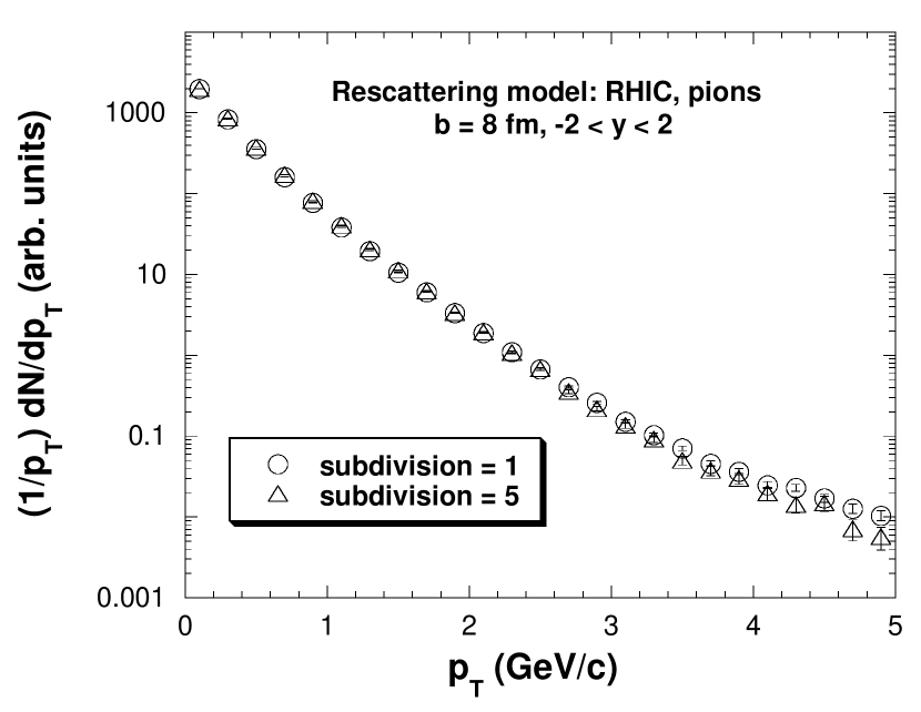
Figure 2: Pion $p_{t}$ distributions for $l=1$ and $l=5$, from ref. Humanic:2005ye . The insensitivity of the transverse momentum distribution to the number of subdivisions indicates that the scaling properties of the transport equations are satisfied by the HRC code. Similar subdivision tests are satisfied by the HRC code for the elliptic flow as a function of the transverse momentum $v2(p_{t})$, the elliptic flow as a function of the longitudinal angular variable $\eta$ as $v_{2}(\eta)$, see ref. Humanic:2005ye for further details.

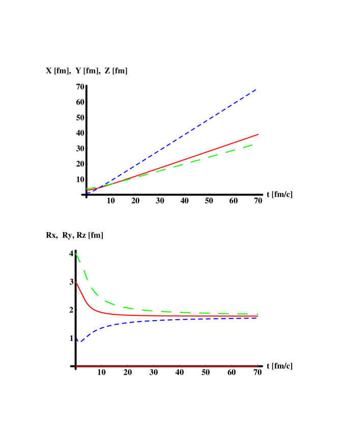
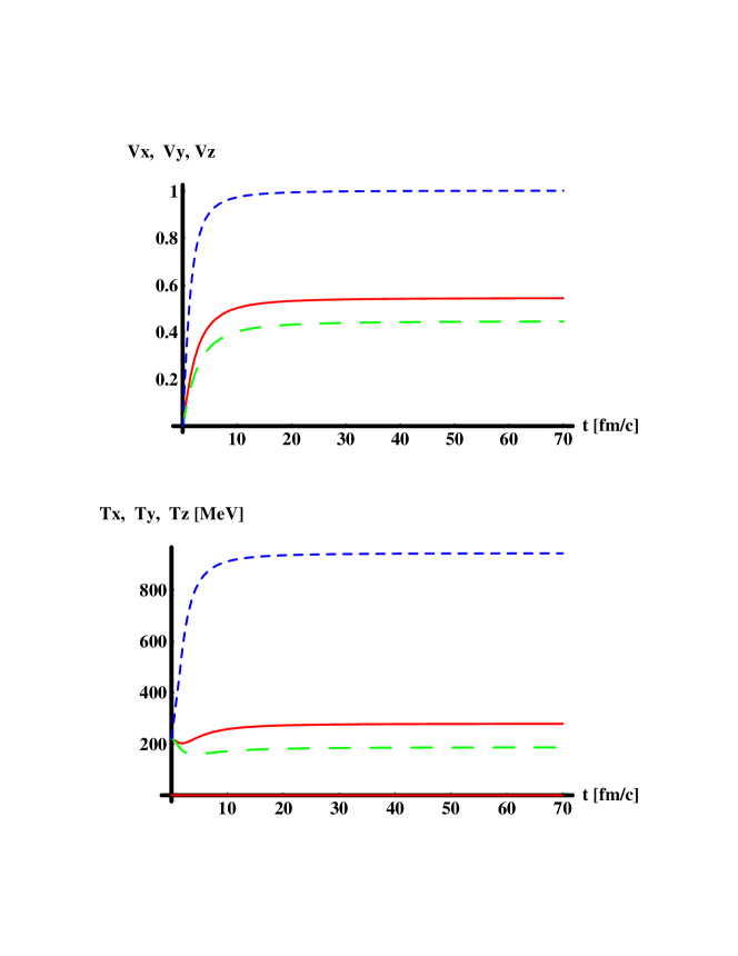
Figure 3: Time evolution of an expanding ellipsoid with Gaussian density profile and homogeneous temperature profile in Buda-Lund type of exact solutions of non-relativistic hydrodynamics. $(X,Y,Z)$ stand for the principal axis of this expanding ellipsoid, after an initial acceleration, these scales evolve linearly with time (top). The corresponding HBT radii, $(R_{x},R_{y},R_{z})$ approach a direction independent constant (below top). The expansion velocities of the principal axis of the exploding ellipsoid, $(V_{x},V_{y},V_{z})$ tend to direction dependent constants (above bottom panel) and similarly, the slope parameters of the single particle spectra in the principal directions, $(T_{x},T_{y},T_{z})$ also tend to direction independent constants (bottom panel). Based on ref. Csorgo:2002kt .

Figure 4: Time evolution of $v_{2}$, HBT, and $m_{T}$ slope parameters from HRC for RHIC Au+Au, from ref Humanic:2005ye . The HRC code shows the same self-quenching properties as the Buda-Lund type of exact solutions of non-relativistic hydrodynamics.

V.2 Self-consistency criteria - subdivision test

The self-consistency check of subdivision invariance is based on the invariance of the Boltzmann equation, the basis of the Monte Carlo particle-scattering calculations, for a simultaneous decrease of the scattering cross sections by some factor  $l$, and an increase of the particle density by the same factor of $l$Zhang:1998a . As $l$ becomes sufficiently large, non-causal artifacts become insignificant. The HRC rescattering calculations have been tested by comparing pion observables for no-subdivision, i.e. $l=1$, with subdivision of $l=5$. Descriptions of how the observables are extracted from the rescattering calculation are given elsewhere Humanic:2002a .

All calculations were carried out for an impact parameter of 8 fm, to simulate semi-central collisions, that result in significant elliptic flow. Such HRC results Humanic:2005ye reproduced reasonably well the RHIC data on the corresponding observables in Au+Au collisions at $\sqrt{s_{NN}}=200$ GeV. Thus this HRC code passed not only the test of reproducing the important global observables, but also the subdivision test, which suggests that there are no significant programming artifacts, or causality violating terms in this Monte Carlo simulation code. Fig. 2 (taken from ref. Humanic:2005ye ) shows a comparisons of the $l=1$ and the $l=5$ cases utilizing the HRC model to describe the charge averaged pion spectra. Similar plots were published for the HBT radius parameters and the transverse momentum and pseudorapidity $\eta$ dependence of the elliptic flow. See ref. Humanic:2005ye for further details and for the comparison plots with RHIC Au+Au data.

V.3 Self-consistency criteria - comparison with exact hydrodynamical results

Motivated by the success of the Buda-Lund parameterization  Csorgo:1995bi ; Csanad:2003qa of the hadronic final state, a search started to find parametric, but time dependent, exact solutions of hydrodynamics, that lead to Buda-Lund type of nearly Gaussian freeze-out distributions. Surprisingly large classes of exact, parametric solutions of hydrodynamics have been recently found this way, both in the non-relativistic  Csorgo:2001ru ; Csorgo:2001xm ; Csorgo:2002kt as well as in the relativistic  Biro:1999eh ; Csorgo:2003ry ; Csorgo:2003rt ; Sinyukov:2004am ; Csorgo:2006ax ; Pratt:2006jj kinematic domain.

These generalized, Buda-Lund type parametric, hydrodynamical calculations have a built-in self-quenching effect, as analyzed in detail in ref. Csorgo:2002kt . For example, all the HBT radii stop to evolve in time, they approach a direction independent constant, and expansion velocities tend to direction dependent constants, although the system keeps on expanding (via rescattering process or hydrodynamical evolution). Elliptic flow also freezes out at the same time when the spectra (slopes) stop to evolve in time. These general, qualitative properties of exact parametric hydrodynamic solutions are illustrated in Fig. 3. In ref. Csorgo:2002kt we have shown that this self-quenching is a general property of a large class of exact analytic hydrodynamic solutions, which is independent of the particular initial conditions - a beautiful exact result. This property of the exact non-relativistic ellipsoidal hydrodynamic solutions is beautifully reproduced in the Hadronic Resonance Model, as shown on Fig. 4.

V.4 More than hydro - tails of particle production

As summarized above the HRC resonance cascade model describes well the observables in heavy ion collisions at both CERN SPS and at RHIC energies, and it passes the subdivision test, and yields such a time evolution of the observables, which is similar to the analytically obtained, exact hydrodynamical asymptotic behavior of these observables. So HRC looks to be a reliable model for the production of the bulk of the particles. In the subsequent part, we investigate if the HRC model is able to describe also the tails of the particle production in $\sqrt{s_{NN}}=200$ GeV Au+Au collisions.

It turns out that this conventional hadronic cascade model HRC has a built-in adaptive bin size in the time direction, hence there is no built-in cutoff time scale in the code. HRC also contains the cascading of the most abundant hadrons: $\rho$, $\Delta$, K^∗, $\omega$, $\eta$, $\eta^{\prime}$, $\phi$ and $\Lambda$, but it neglects electrical charge. Therefore we see that this HRC model implements rescattering in a time dependent mean free path system, and in the previous section we have shown that under certain conditions this corresponds to a random Lévy walk and is signaled by power-law tails in the source distribution. Let’s see whether the HRC simulation results confirm such an expectation or not.

VI DETAILED HRC SIMULATION RESULTS

We generated 48 events with b=4.45 fm and 5730 events with 12.5 fm corresponding to the 0-20% and 50-90% centrality classes of PHENIX events. The generated events have average multiplicities of 3400 and 38 particles, respectively. The mean impact parameter values suiting the two centralities were determined from a Glauber calculation as in ref. Adler:2003au .

We made cuts on the data sample similar to the ones in the PHENIX imaging paper PHENIX-imaging :

• 0-20% and 0.2 GeV$/c\;<p_{t}<\;$0.36 GeV$/c$,

• 0-20% and 0.48 GeV$/c\;<p_{t}<\;$0.6 GeV$/c$,

• 40-90% and 0.2 GeV$/c\;<p_{t}<\;$0.4 GeV$/c$,

in addition to the PHENIX geometry cut of $-0.5<y<0.5$.

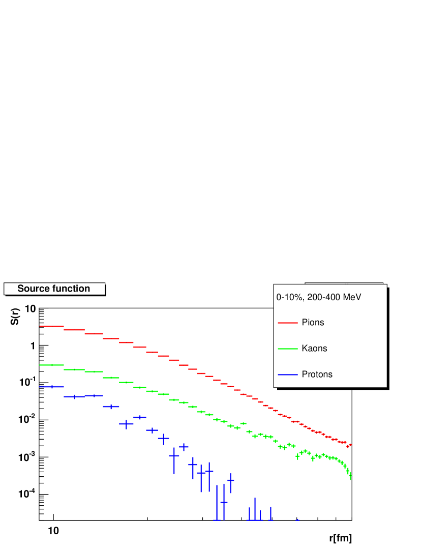
Figure 20: Source distribution of pion, kaon and proton pairs with 0.2 GeV$/c$ $<p_{t}<$ 0.4 GeV$/c$ and 0-10% centrality.

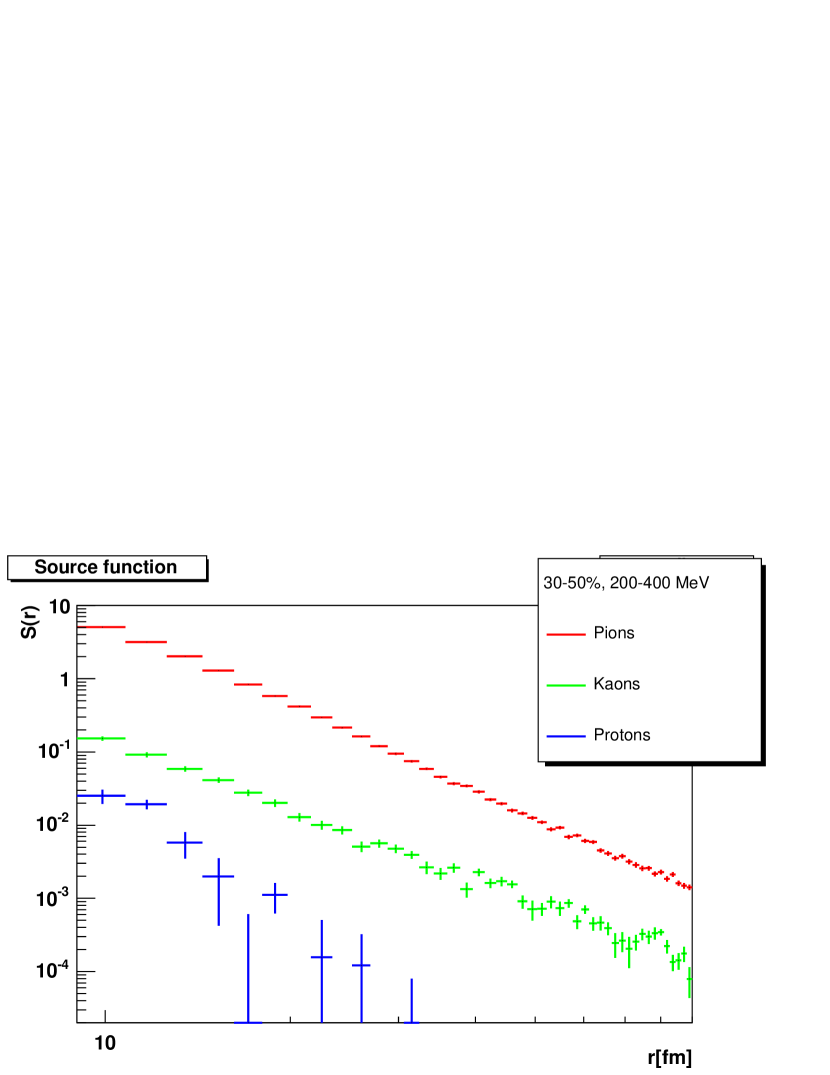
Figure 21: Source distribution of pion, kaon and proton pairs with 0.2 GeV$/c$ $<p_{t}<$ 0.4 GeV$/c$ and 30-50% centrality.

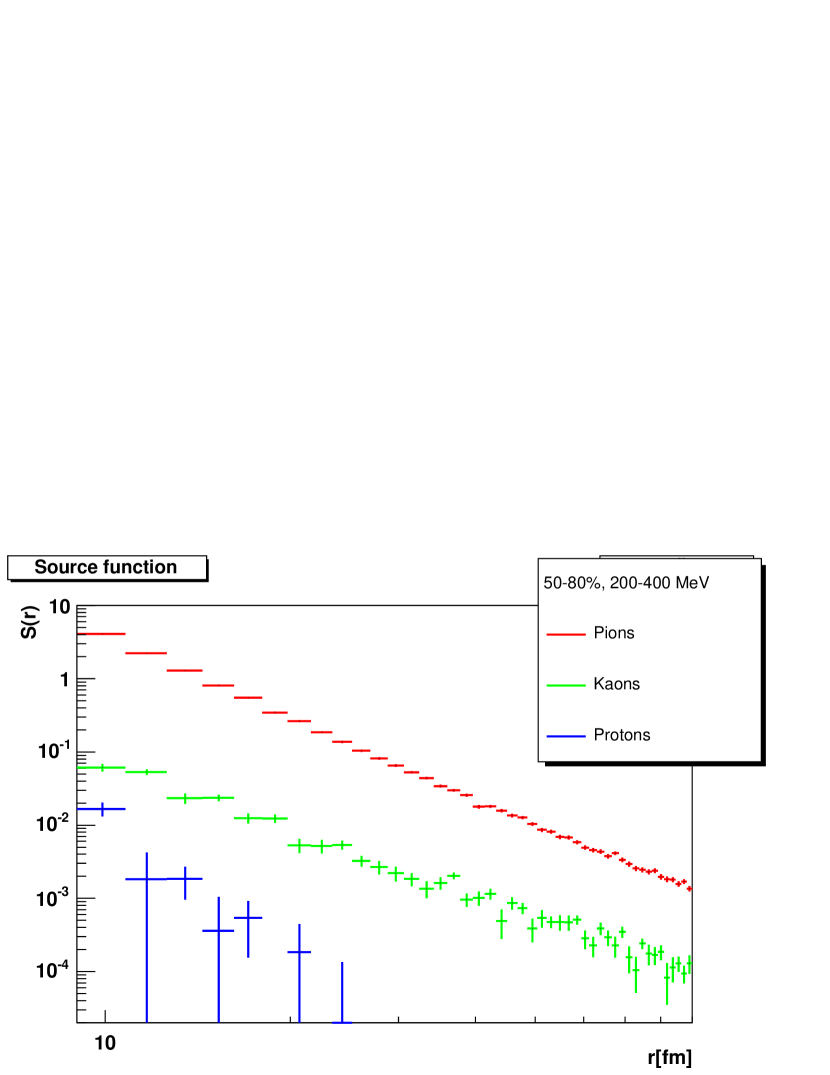
Figure 22: Source distribution of pion, kaon and proton pairs with 0.2 GeV$/c$ $<p_{t}<$ 0.4 GeV$/c$ and 50-80% centrality

The resulting plots are shown in Figs. 5-22. The complete source function is decomposed to different components, i.e. the $S(r)$ distributions created from pairs with both pions being

• primordial or decay products of resonances that have a lifetime less than 20 fm$/c$; this means here direct pions $\rho$, $\Delta$, K^∗ decay products, referred to as core, or c pions;

• decay products of an $\omega$

• decay products of resonances that have a lifetime greater than 25 fm$/c$; in HRC: $\Lambda$, $\Phi$, $\eta$, $\eta^{\prime}$, referred to as halo or h pions.

One of the pions in a pair is from one above category, and the other may be from another one: so in this study we distinguish $(c,c)$, $(c,\omega)$, $(c,h)$, $(\omega,\omega)$, $(\omega,h)$ and $(h,h)$ type of possible combinations.

VI.1 HRC simulations and PHENIX data

In this subsection we compare the HRC model calculations with experimental data from PHENIX-imaging . The kinematic cuts correspond to Figs. 1a,b and Fig.2 of ref. PHENIX-imaging .

The PHENIX imaged $S(r)$ source distribution coincides with the HRC simulation result, and both are describable with a power-law tail, in the kinematic region of 0-20% centrality and 0.2 GeV$/c<p_{t}<$ 0.36 GeV$/c$, for pion pairs, as indicated in Fig. 5. On this log-log plot, the tail of $S(r)$ is approximately linear, so it can well be called a heavy tail. Clearly a further refinement of the experimental resolution could reveal more details on the structure of this tail behavior, but a power-law approximation is not inconsistent with the currently available data.

In HRC, this power-law tail is due to rescattering because of the adaptive time-scale, corresponding to anomalous diffusion. This results in Levy distributions, in contrast to Gaussian distributions, which clearly fail to reproduce the tails of the particle production. The Lévy index of stability, $\alpha$, can be determined approximately from fits to the tails of these $S(r)$ source functions: as for Lévy sources $S(r)\propto r^{-(d+\alpha)}$ in $d$ spatial dimensions. In the HRC simulations, as well as in case of $S(r)$ reconstructed by PHENIX, $d=3$. From Fig. 5, the HRC simulations and PHENIX data both indicate a Lévy index of stability of $\alpha\approx 1.15\pm 0.1$, which is consistent with the direct Lévy fits to PHENIX preliminary Coulomb corrected correlation functions in a similar kinematic region, as presented in ref. Csanad:2005nr .

This is a great success of the HRC model, as it seems that it has implemented the key effect, the anomalous diffusion, reasonably well to the simulation.

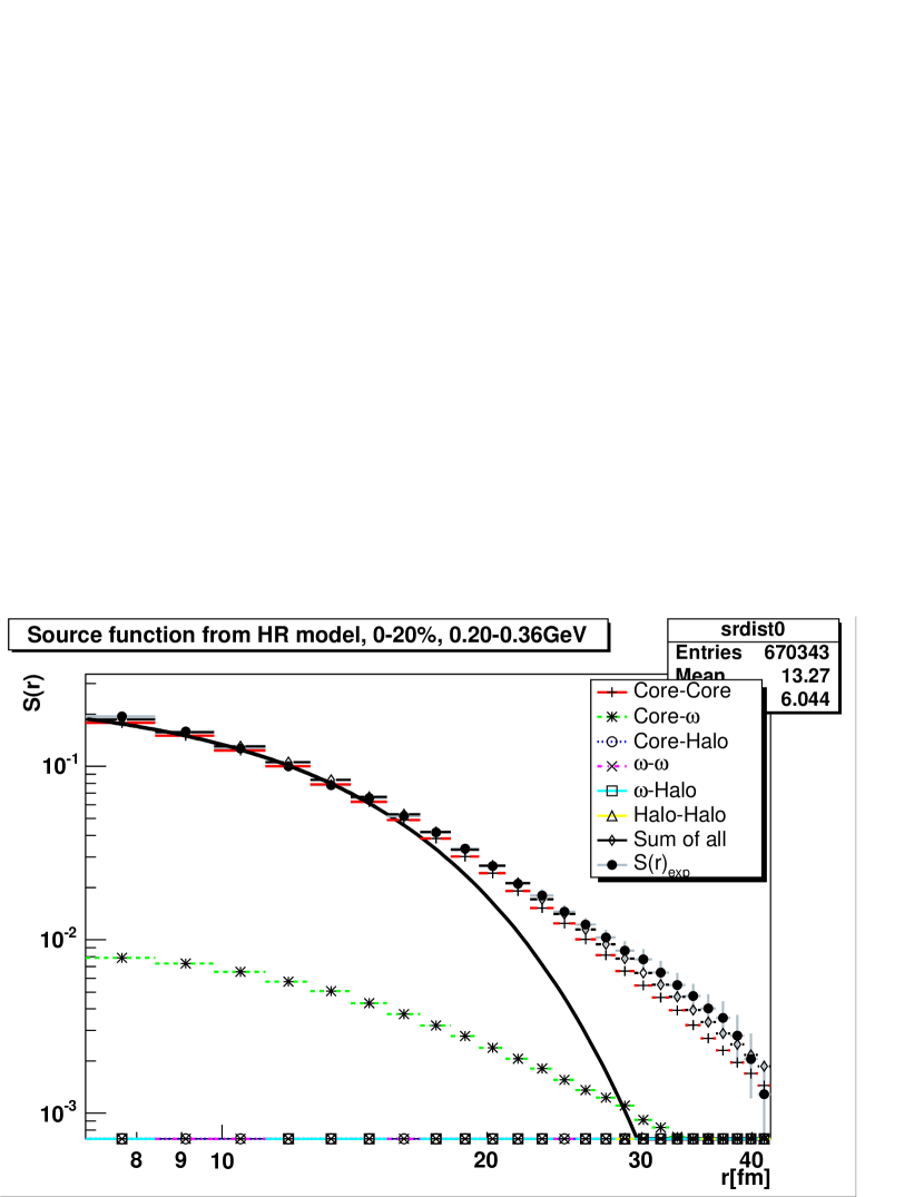
Figure 5: Pions for 0-20% centrality and 0.2 GeV$/c<p_{t}<$ 0.36 GeV$/c$, with the various components of the source. On the length scales less than 50 fm, core-core pairs are the most abundant ones in the present situation. The next to largest contribution is from the $(c,\omega)$ pairs, however, their contribution of is very small as compared to the core-core pairs in the experimentally resolvable region, all the other contributions are negligible. A comparison of the full HRC simulation result (open diamonds) with PHENIX data PHENIX-imaging (filled circles, $S(r)_{exp}$) indicates that HRC model simulations are in a good agreement with data in this kinematic range. Solid black line shows the best Gaussian fit to $S(r)$ in the 0 fm $<r<$ 15 fm region, which misses the tail region clearly.

Let us investigate in greater detail if HRC can describe more subtle features of the PHENIX data. In Fig. 6, we show a comparison with data in a similarly soft domain but in the more peripheral centrality class.

Within errors, the HRC simulations again reproduce the PHENIX measured $S(r)$ source functions, even if the experimental statistics does not allow for a comparison in the interesting region of $r>20$ fm. The HRC simulations, which have better statistics than the experimental data, indicate a power-law tail with similar exponent as in the case of more central collisions. From the comparison with the previous figure it follows that the HRC model describes the centrality dependence of the heavy tail in this soft $k_{t}$ region in an acceptable manner. This is yet another feature of the HRC model which deserves appreciation.

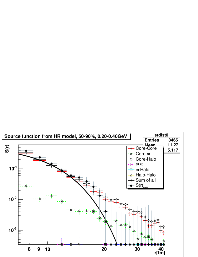
Figure 6: Same as the previous figure, but for a 50-90% centrality and 0.2 GeV$/c<p_{t}<$ 0.40 GeV$/c$ kinematic selection. HRC simulations are shown with the various components of the HRC source resolved. A comparison with PHENIX data PHENIX-imaging (filled circles, $S(r)_{exp}$) indicates that HRC model simulations are in an agreement with facts in this kinematic range, too, although within errors, systematic deviations between the simulation results and PHENIX data can be observed in the $r>20$ fm region.

Let us now investigate how well can a HRC simulation describe the transverse momentum dependence of the relative coordinate distributions of pion pairs. Such a comparison is shown in Fig. 7. In the 0-20% centrality and 0.48 GeV$/c<p_{t}<$ 0.60 GeV$/c$ kinematic selection, the HRC model simulations are in a disagreement with PHENIX data. So the HRC model does not describe the observed transverse momentum dependence of the PHENIX imaged source distribution in case of nearly central collisions. Although the achievements of this model are really impressive, in this kinematic region the model could be improved or fine-tuned. In fact it seems that rescattering effects are too large as compared to data with increasing transverse momentum.

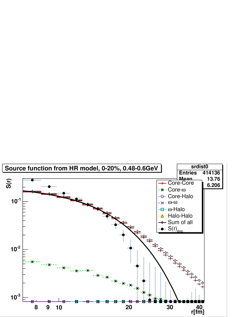
Figure 7: Same as the previous figures, but for a 0-20% centrality and 0.48 GeV$/c<p_{t}<$ 0.60 GeV$/c$ kinematic selection. HRC simulations are shown with the various components of the HRC source resolved. The HRC model simulations are in a disagreement with PHENIX data in this kinematic range.

In the subsequent parts, we explore the HRC model predictions in greater detail. We focus our attention to the tails of particle production, and try to identify within the limitations of this model calculation what kind of experimental control is available for changing the exponent (or, on a log-log plot, the slope parameter) of the tails of particle emission in the HRC simulations. This is motivated by the recent predictions in ref. 2ndQCD that suggested the existence of a power-law tail in the coordinate space distribution at the critical end point of the line of first order phase transitions in QCD. At this critical point the phase transition is of second order, and the Bose-Einstein correlation function has a Lévy form, with the Lévy index of stability coinciding with the correlation exponent $\eta$ that is one of the critical exponents, and its value is universal, depending only on the universality class of the second order phase transition. Hence in a second order QCD phase transition the Lévy index of stability or the power-law exponent of the tails of the particle production becomes independent of the momentum range, centrality selection, and the particle type. However, in case of anomalous diffusion of hadrons the rescattering might well be sensitive to the centrality that drives multiplicity and particle densities, the momentum range that also influences how many particles take part in the rescattering process and also the particle type, as the number of rescatterings is expected to depend on the particle cross sections.

VI.2 Centrality dependence of the HRC source

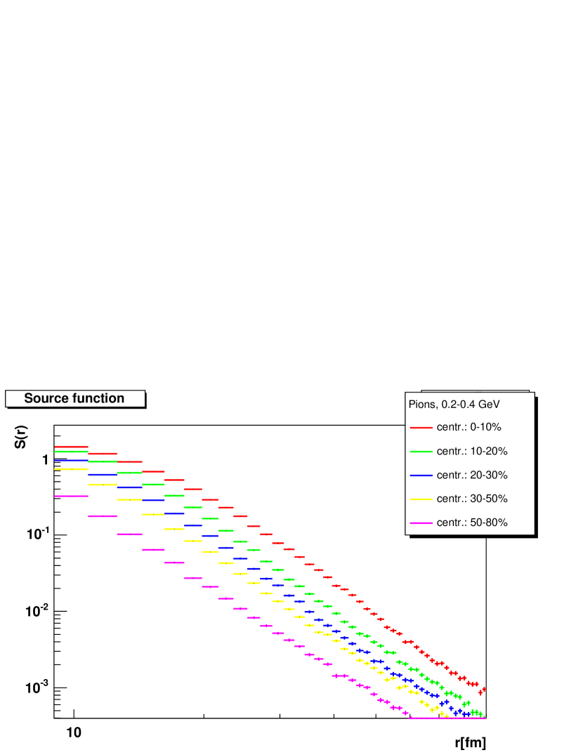
Figure 8: Source distribution of HRC simulated pion pairs with 0.2 GeV$/c$ $<p_{t}<$ 0.4 GeV$/c$ for various centrality classes.

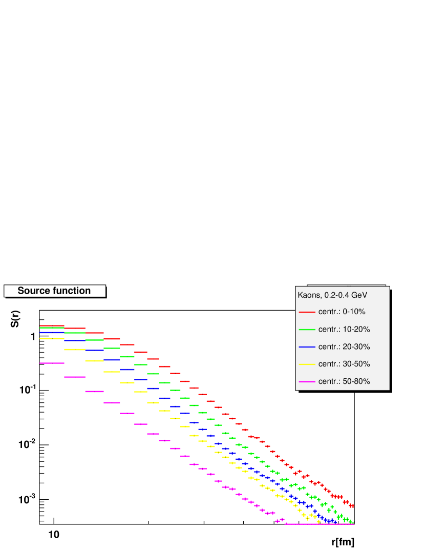
Figure 9: Source distribution of HRC simulated pion pairs with 0.5 GeV$/c$ $<p_{t}<$ 1.0 GeV$/c$ for various centrality classes.

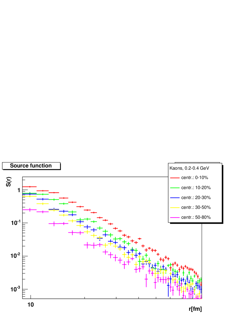
Figure 10: Source distribution of kaon pairs with 0.2 GeV$/c$ $<p_{t}<$ 0.4 GeV$/c$ for various centrality classes.

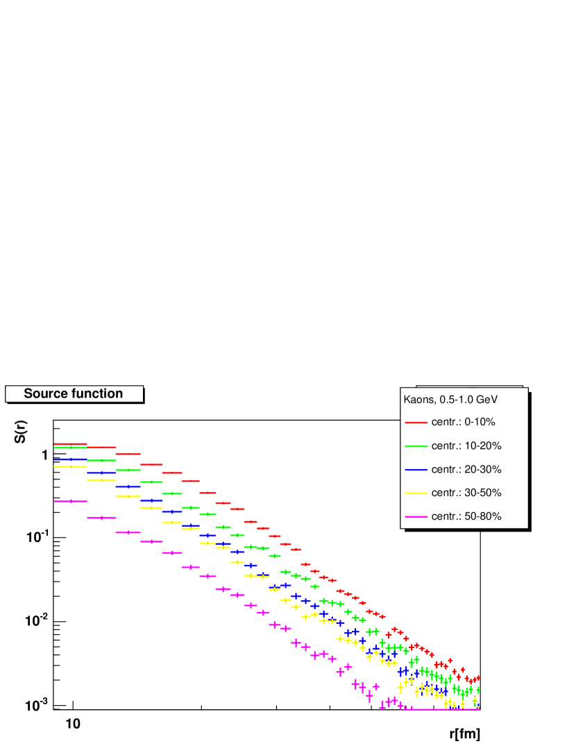
Figure 11: Source distribution of kaon pairs with 0.5 GeV$/c$ $<p_{t}<$ 1.0 GeV$/c$ for various centrality classes.

The centrality dependence of the HRC simulated source distributions of pions with various pair transverse momenta is shown in Figs. 8-13. The centrality dependence of the tails of particle emissions is found to be surprisingly small, as on the log-log plots the tails corresponding to various centrality selections in Figs. 8-13 are found to be parallel. The centrality selection, however, sensitively influences the region of bulk particle production, corresponding to the change of the scale parameters or the effective source sizes in the small $r$ region. The slope of the tails in this simulation, however, is independent of centrality for pions at low or higher transverse momentum, Figs. 8-9, as well as for low or higher momentum kaons, Figs. 10-11, and for protons, Figs. 12-13. Although in case of the proton sources statistical limitations prevent us from firm conclusion, it seems that the power-law exponent of the tails of particle emission is rather insensitive to the centrality selection, regardless of particle type and pair momentum selection, so centrality is not a sensitive control tool to separate heavy tails that arise due to anomalous diffusion from heavy tails that appear due to the vicinity of a second order QCD phase transition.

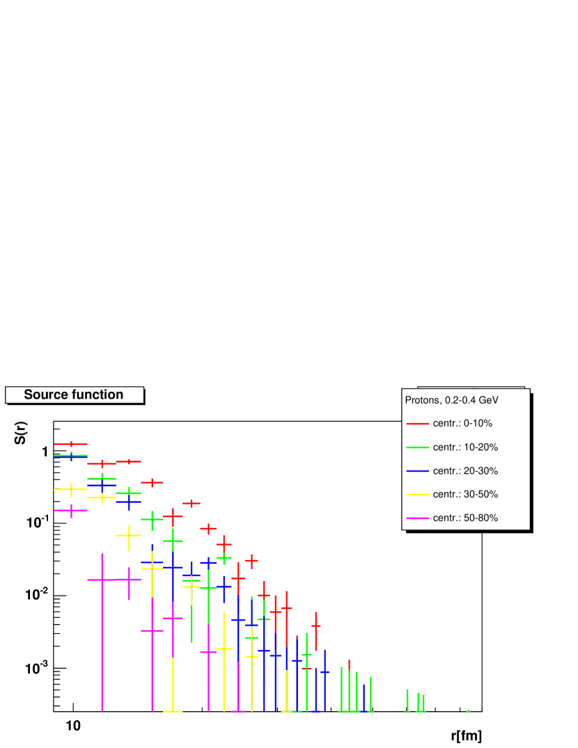
Figure 12: Source distribution of proton pairs with 0.2 GeV$/c$ $<p_{t}<$ 0.4 GeV$/c$ for various centrality classes.

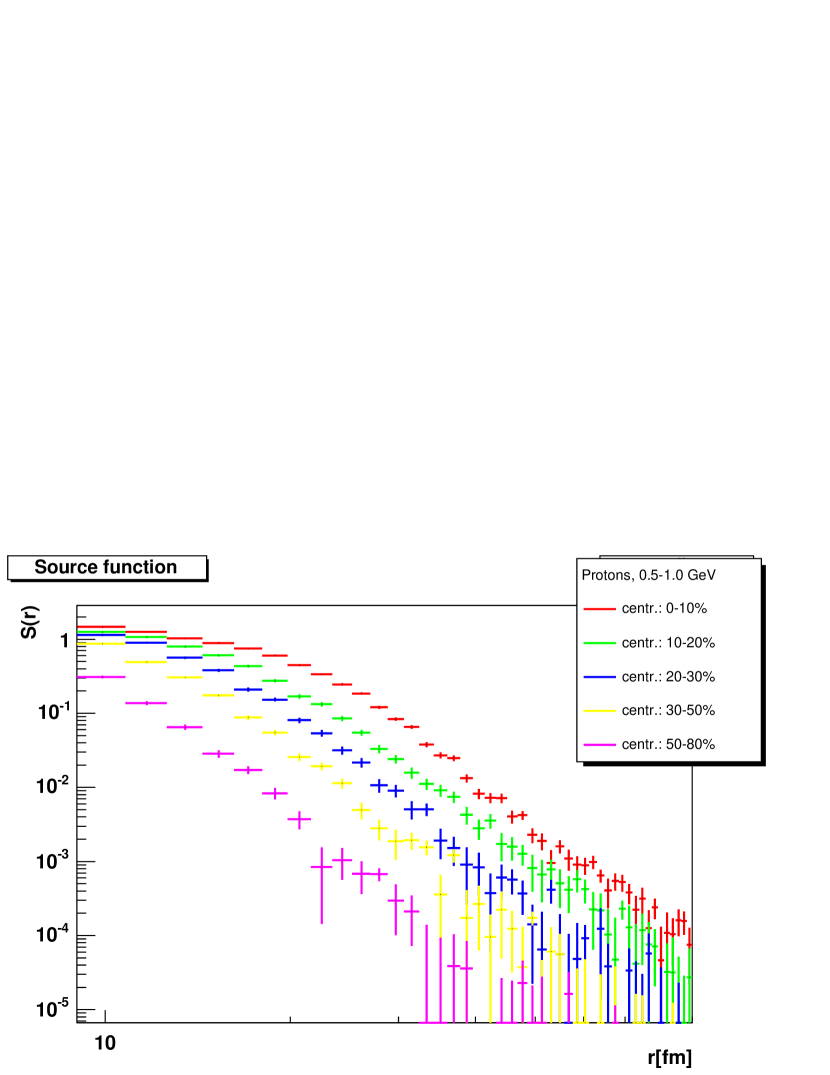
Figure 13: Source distribution of proton pairs with 0.5 GeV$/c$ $<p_{t}<$ 1.0 GeV$/c$ for various centrality classes.

VI.3 Transverse momentum dependence

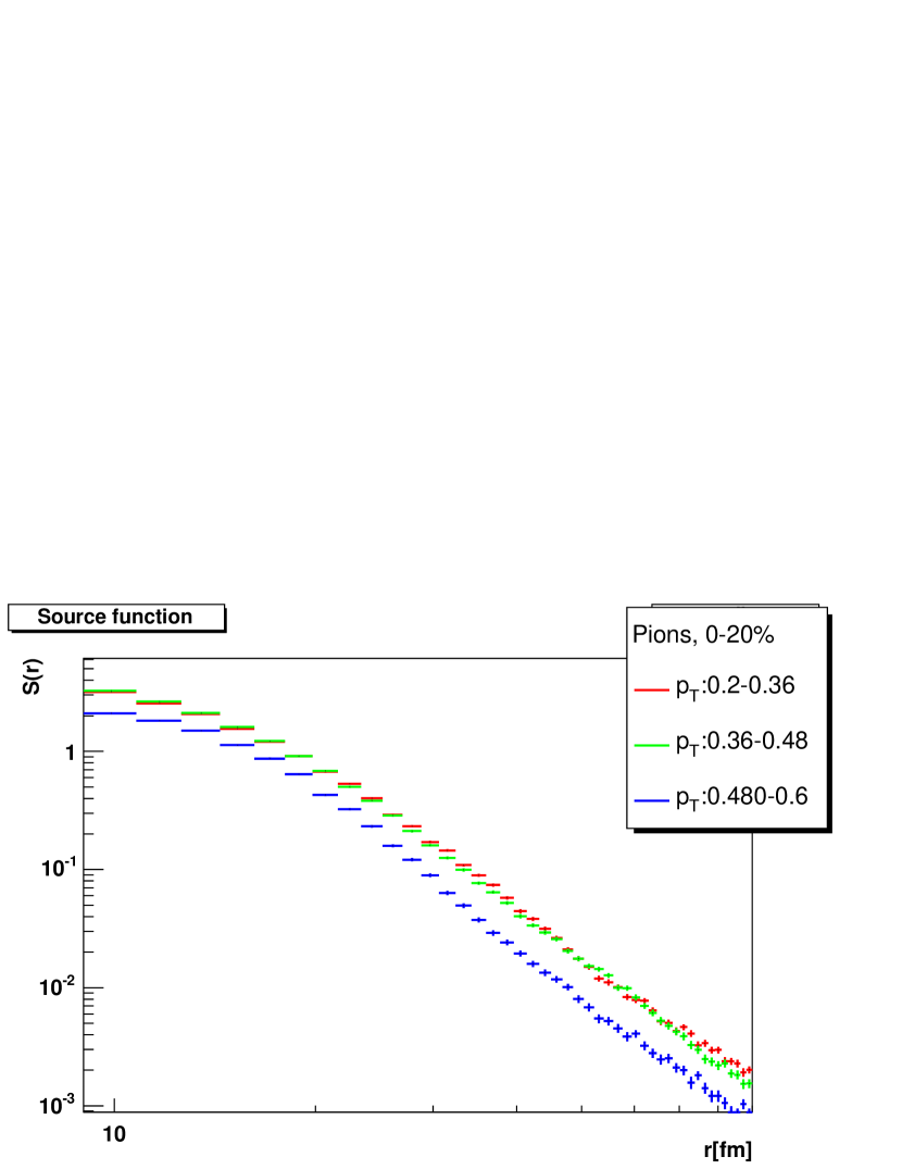
Figure 14: Source distribution of pion pairs with 0-20% centrality, for various $p_{t}$ ranges

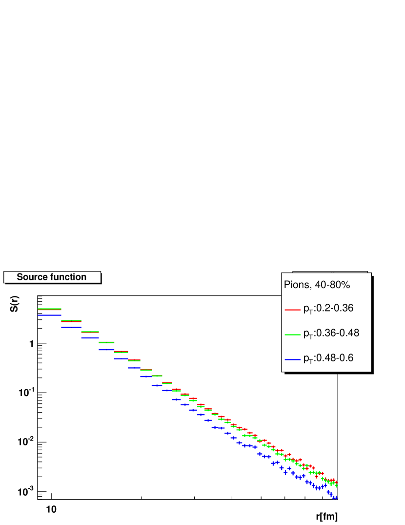
Figure 15: Source distribution of pion pairs with 40-80% centrality, for various $p_{t}$ ranges

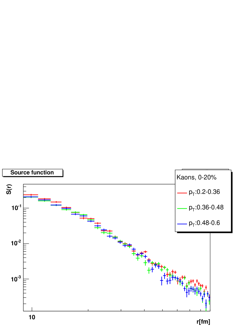
Figure 16: Source distribution of kaon pairs with 0-20% centrality, for various $p_{t}$ ranges

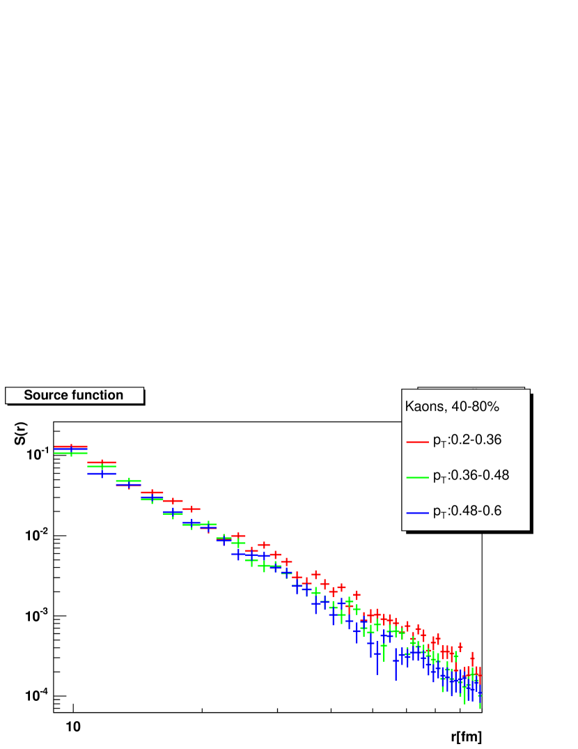
Figure 17: Source distribution of kaon pairs with 40-80% centrality, for various $p_{t}$ ranges

Transverse momentum dependence of simulated source distributions in various centrality classes is shown in Figs. 14-19. For nearly central collisions and pions, the increase of the transverse momentum of the pair reduces the size of the bulk production region, as was well known from earlier Bose-Einstein correlation measurements and theoretical explanations, see e.g. refs. Csorgo:1995bi ; Csanad:2003qa . Being aware of the strong transverse momentum dependences of the scale parameter $R$, which is well shown by the HRC simulation, it is rather surprising, that the shape parameter of the tail, the Lévy index of stability $\alpha$ is remarkably insensitive to the selected transverse momentum regions, which follows from the fact that on the log-log plot the simulated $S(r)$ tails are parallel to one another, see Fig. 14. The same effect is shown in Fig. 15, in case of peripheral collisions. For kaons, the evolution of the source function is less apparent in the same transverse momentum regions, this is due to the fact that the effective radius parameters, the scales in analytic calculations like of refs. Csorgo:1995bi ; Csanad:2003qa , are found to be predominantly depending on the transverse mass, $m_{t}=\sqrt{m^{2}+p_{t}^{2}}$ of the particles. The same variation in the transverse momentum $p_{t}$ leads to a larger variation in $m_{t}$ for pions, as compared to that of kaons, due to the larger value of the kaon mass: $m_{\pi}\approx 140$ MeV, while $m_{K}\approx 494$ MeV. This explains why Figs. 16 and  17 show remarkably small variations of the kaon emitting source with increasing values of the transverse momenta of kaons. In case of protons, one would expect even smaller variations with increasing momentum, however, in this case the Monte Carlo simulations indicate an increase of the effective source size with increasing momentum. Even in case of protons the dependence of the power-law exponent on the transverse momentum is negligible. Thus the transverse momentum dependence of the power-law exponent $\alpha$ is negligible in each considered case.

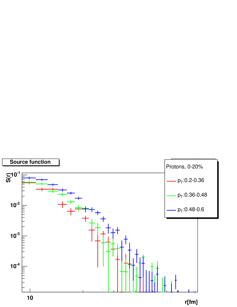
Figure 18: Source distribution of proton pairs with 0-20% centrality, for various $p_{t}$ ranges

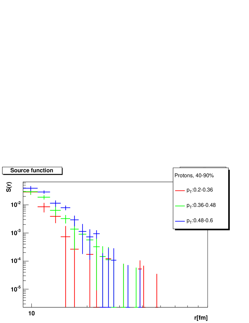
Figure 19: Source distribution of proton pairs with 40-80% centrality, for various $p_{t}$ ranges

VI.4 Particle type dependence

Particle type dependence of simulated source distributions in various centrality classes and with a pair transverse momentum of 0.2 GeV$/c$ $<p_{t}<$ 0.4 GeV$/c$ is shown in Figs. 14-19. These source distributions all have an approximate power-law tail, as expected in case of an anomalous diffusion effect. However, the power-law exponents have rather different values for different particle types. This is well understandable as the total inelastic cross sections of these particles are rather different. Protons have the largest cross sections, pions the second largest, and kaons the smallest. Hence the protons have the shortest mean free path, the pions the second shortest, and the kaons have the largest mean free path at any given densities. This implies that the heaviest tail develops for kaons, the second heaviest tail for pions, and the proton source distribution is closest to the Gaussian distribution. However, it is rather difficult to make such a simple picture given that the HRC simulation includes a parameterized form of the strongly momentum dependent cross sections, when available, it uses Particle Data Group tables PDG92 , although not the most recent version of these tables PDG06 . Whenever PDG data were not available, the HRC model utilized theoretical results on the total cross sections from Prakash, Prakash, Venugopalan and Welke Prakash:1993bt .

VII CONCLUSIONS AND SUMMARY

A power-law tail of the relative coordinate distribution $S(r)$ appears in HRC model simulations for Au+Au collisions at RHIC energies. The simulation reproduces an important feature of recent PHENIX experimental data on heavy tails, i.e. it yields a power-law tail with an exponent, or Lévy index of stability of $\alpha\approx 1.3\pm 0.1$. Detailed simulation results indicate that this exponent (as well as the tails of the $S(r)$ relative coordinate distribution) depends strongly on the particle cross sections or particle type, while for a given particle type it is remarkably insensitive to centrality and momentum selections, which implies insensitivity to the actual number of collisions. The exponent value is rather different from $\alpha\approx 0.5$ predicted for the second order QCD phase transition in ref. 2ndQCD . Also, at a second order QCD phase transition, the exponents are determined from universality class arguments, so in case of a second order phase transition, no particle type dependence is expected. Hence measuring the tails of particle production for protons and kaons seems to be a promising method to distinguish between a second order QCD phase transition and anomalous diffusion.

The Lévy distribution is called stable because the convolution of two such distribution is also a Lévy distribution. In addition, the generalized central limit theorem says that the convolution of many (in the limiting case infinitely many) elementary processes with the same (but arbitrary) probability distribution is a Lévy stable distribution. So it is natural, although still surprising that Lévy stable, power-law tailed source distributions appear in the HRC model simulations. (The rescattering can be considered as such elementary process.)

The extraction of the precise values of the power-law exponents, or the Lévy index of stability, with reliable experimental statistical and systematic errors is an important future task that allows experimental characterization of anomalous diffusion or second order QCD phase transitions with a simple number. Measuring the transverse momentum, centrality, and particle type dependence of this exponent tells a lot about the production mechanism of particles in high energy heavy ion collisions. In particular, measuring the Lévy index of stability for pions, kaons, and protons can serve as a promising experimental control possibility on the origin of the heavy tailed distribution.

Acknowledgments: We are grateful to professor Tom Humanic for forwarding his HRC simulation code to us. T. Cs. would like to express his deep gratitude to professors S.S. Padula, Y. Hama and M. Hussein for the kind invitation and hospitality and for their organizing a series of outstanding conferences in Brazil.

References

- (1) R. Lednicky, Nucl. Phys. A 774 (2006) 189 [arXiv:nucl-th/0510020].
- (2) S. S. Padula, Braz. J. Phys. 35, 70 (2005) [arXiv:nucl-th/0412103].
- (3) T. Csörgő, J. Phys. Conf. Ser. 50, 259 (2006) [arXiv:nucl-th/0505019].
- (4) M. A. Lisa, S. Pratt, R. Soltz and U. Wiedemann, Ann. Rev. Nucl. Part. Sci. 55, 357 (2005) [arXiv:nucl-ex/0505014].
- (5) M. Lisa, AIP Conf. Proc. 828, 226 (2006) [arXiv:nucl-ex/0512008].
- (6) R. C. Hwa, arXiv:nucl-th/0701053.
- (7) S. S. Adler et al. [PHENIX Collaboration], arXiv:nucl-ex/0605032.
- (8) A. Białas, Acta Phys. Polon. B 23, 561 (1992).
- (9) R. Metzler, J. Klafter, Physics Reports 339 (2000) 1-77
- (10) T. J. Humanic, Int. J. Mod. Phys. E 15, 197 (2006) [arXiv:nucl-th/0510049].
- (11) V. V. Uchaikin and V. M. Zolotarev, “Chance and Stability, Stable Distributions and Their Applications”, VSP Science,1999, ISBN: 90-6764-301-7, 596 pp.
- (12) V. M. Zolotarev, “One-dimensional Stable Distributions”, Am. Math. Soc. Transl. of Math. Monographs, vol. 65, Providence, R.I. (Transl. of the original 1983 Russian)
-
(13)
J. P. Nolan, Stable Distributions: Models for Heavy Tailed Data
http://academic2.american.edu/jpnolan/stable/CHAP1.PDF - (14) Nolan, J. P. Stable Distributions: Models for Heavy Tailed Data. Boston, MA: Birkh user, 2005
- (15) T. Csörgő, S. Hegyi and W. A. Zajc, Eur. Phys. J. C 36, 67 (2004) [arXiv:nucl-th/0310042].
- (16) J. Adams et al. [STAR Collaboration], Phys. Rev. C 71, 044906 (2005) [arXiv:nucl-ex/0411036].
- (17) D. A. Brown and P. Danielewicz, Phys. Lett. B 398, 252 (1997) [arXiv:nucl-th/9701010].
- (18) T. J. Humanic, arXiv:nucl-th/0301055.
- (19) B. Zhang, C. M. Ko, B. A. Li and Z. w. Lin, Phys. Rev. C 61, 067901 (2000) [arXiv:nucl-th/9907017].
- (20) T. J. Humanic, arXiv:nucl-th/0205053.
- (21) C. M. Ko, Z. W. Lin and S. Pal, Heavy Ion Phys. 17, 219 (2003) [arXiv:nucl-th/0205056].
- (22) B. Zhang, M. Gyulassy and Y. Pang, Phys. Rev. C 58, 1175 (1998)
- (23) T. Csörgő and B. Lörstad, Phys. Rev. C 54, 1390 (1996) [arXiv:hep-ph/9509213].
- (24) M. Csanád, T. Csörgő and B. Lörstad, Nucl. Phys. A 742, 80 (2004) [arXiv:nucl-th/0310040].
- (25) T. Csörgő, Acta Phys. Polon. B 37, 483 (2006) [arXiv:hep-ph/0111139].
- (26) T. Csörgő, S. V. Akkelin, Y. Hama, B. Lukács and Yu. M. Sinyukov, Phys. Rev. C 67, 034904 (2003) [arXiv:hep-ph/0108067].
- (27) T. Csörgő and J. Zimányi, Heavy Ion Phys. 17, 281 (2003) [arXiv:nucl-th/0206051].
- (28) T. S. Biró, Phys. Lett. B 474, 21 (2000) [arXiv:nucl-th/9911004].
- (29) T. Csörgő, L. P. Csernai, Y. Hama and T. Kodama, Heavy Ion Phys. A 21, 73 (2004) [arXiv:nucl-th/0306004].
- (30) T. Csörgő, F. Grassi, Y. Hama and T. Kodama, Phys. Lett. B 565, 107 (2003) [arXiv:nucl-th/0305059].
- (31) Yu. M. Sinyukov and I. A. Karpenko, Acta Phys.Hung. A25, 141-147 (2006) [arXiv:nucl-th/0506002].
- (32) T. Csörgő, M. I. Nagy and M. Csanád, arXiv:nucl-th/0605070.
- (33) S. Pratt, arXiv:nucl-th/0612010.
- (34) S. S. Adler et al. [PHENIX Collaboration], Phys. Rev. C 69, 034910 (2004) [arXiv:nucl-ex/0308006].
- (35) M. Csanad [PHENIX Collaboration], Nucl. Phys. A 774, 611 (2006) [arXiv:nucl-ex/0509042].
-
(36)
T. Csörgő, S. Hegyi, T. Novák and W. A. Zajc,
AIP Conf. Proc. 828, 525 (2006)
[arXiv:nucl-th/0512060];
T. Csörgő, S. Hegyi, T. Novák and W. A. Zajc, Acta Phys. Polon. B 36, 329 (2005) [arXiv:hep-ph/0412243]. - (37) K. Hikasa et al., Particle Data Group, Phys. Rev. D 45 (1992) 83
- (38) W-M Yao et al., Particle Data Group, J. Phys. G: Nucl. Part. Phys. 33 (2006) 1-1232
- (39) M. Prakash, M. Prakash, R. Venugopalan and G. Welke, Phys. Rept. 227, 321 (1993).