Peristaltic modes of single vortex in the Abelian Higgs model

Abstract

Using the Abelian Higgs model, we study the radial excitations of single vortex and their propagation modes along the vortex line. We call such beyond-stringy modes peristaltic modes of single vortex. With the profile of the static vortex, we derive the vortex-induced potential, i.e., single-particle potential for the Higgs and the photon field fluctuations around the static vortex, and investigate the coherently propagating fluctuations which corresponds to the vibration of the vortex. We derive, analyze and numerically solve the field equations of the Higgs and the photon field fluctuations around the static vortex with various Ginzburg-Landau parameter $\kappa$ and topological charge $n$. Around the BPS value or critical coupling $\kappa^{2}$=1/2, there appears a significant correlation between the Higgs and the photon field fluctuations mediated by the static vortex. As a result, for $\kappa^{2}$=1/2, we find the characteristic new-type discrete pole of the peristaltic mode corresponding to the quasi-bound-state of coherently fluctuating fields and the static vortex. We investigate its excitation energy, correlation energy of coherent fluctuations, spatial distributions, and the resulting magnetic flux behavior in detail. Our investigation covers not only usual Type-II vortices with $n$=1 but also Type-I and Type-II vortices with $n\in Z$ for the application to various general systems where the vortex-like objects behave as the essential degrees of freedom.

I Introduction

There have been wide interests in the study of the topological objects such as the vortices abrikosov , monopoles monopole ; monopole2 , and instantons polyakov because of their importance for understanding some crucial aspects of the nonlinear field theories Raja ; man . They are not included in the original action manifestly, but appear as the localized finite energy solutions of the nonlinear field equations. These solutions can be classified with the topological number which comes from the topological property of the system. Since the topological objects have spatially localized, finite energy configurations and some topologically conserved charge, it is fascinating to regard them as dynamical degrees of freedom in the system.

One of such objects is the Abrikosov vortex abrikosov in Ginzburg-Landau (GL) theory, which appears as the magnetic flux squeezed by the Cooper-pair condensate. When the external magnetic field applied to the superconductor exceeds some critical strength, the Cooper-pair is dissociated and the node of the Cooper-pair forms a vortex line. The single-valued property of the Cooper-pair around vortex lines leads the quantization of the total magnetic flux, as $e\Phi=2\pi n\ (n\in{\bf Z})$, where $e,\Phi,n$ represent the effective gauge coupling of the Cooper-pair, the total magnetic flux and the topological number, respectively. The topological number $n$ characterizes the topology of the system and we can classify vortices in terms of $n$.

There exist many applications employing the concept of the Abrikosov vortex and its relativistic version, the Nielsen-Olesen vortex Nielsen . One example is the squeezed color-electric flux between the quark and anti-quark in QCD. Nambu Nambu , ’t Hooft 't Hooft and Mandelstam Mandel discussed that there exist the vortices which appear as the color-electric flux tubes squeezed by the condensation of magnetic monopoles. As a result of the color-electric flux squeezing, we can only observe colorless mesons and baryons, which are color singlet bound states of the colored quarks with the bond of the color-electric flux. This scenario is a possible explanation for “color confinement”, which is the experimental fact in hadron physics confinement . The lattice QCD Monte Carlo calculations rothe for ${\rm Q\bar{Q}}$ creutz and 3${\rm Q}$ takahashi ; ichie potentials strongly support the flux tube picture, and show the universality of the string tension of the flux-tube, $\sigma\simeq$ 0.89 GeV, in both ${\rm Q\bar{Q}}$ and 3${\rm Q}$ cases.

An another example is the cosmic string in astrophysics as a seed of the galaxy formation and baryogensis vile . Kibble kibble and Zurek zurek discussed the distribution of the topological defects and their cosmological evolution after the quench of the early Universe and the resulting phase transition. They argued that the cosmic strings as topological defects would produce a characteristic signature in the cosmic microwave background. Following their scenarios, the phase transition dynamics are closely investigated in the numerical simulations using the phenomenological time-dependent GL (TDGL) theory tink in both cases with global symmetry and local gauge symmetry. In particular, in the case of the gauge symmetry, it is discussed that the initial thermal magnetic fluctuations just after the quench play important roles on the later distribution of the vortices such as the clusters of vortices hind ; step . These investigations are closely correlated with the condensed matter physics in a viewpoint to understand the phase transition dynamics, and provide the interesting subjects to link different fields of research.

Now we turn to the dynamical aspects of single vortex as a “pseudo-particle”. For the treatment of the vortex motion, the vortex is usually regarded as one dimensional (1-D) thin object like a string, neglecting the extension perpendicular to the vortex line. Such a treatment is expected to be sufficient when the length of the string is much larger than the length scale in the radial direction. This condition comes from the fact that the excitation energy of string as a 1-D object is typically $\sim\pi/l_{s}$ ($l_{s}$ is the string length). Then, for the vortex with large length, the stringy excitation is more important than radial one with changing its thickness. Even if the above condition is not well-satisfied, we have only to consider extensive modes of the magnetic flux when the Type-II nature is very strong, i.e., the Ginzburg-Landau parameter $\kappa=\delta/\xi$ is very large (Here $\delta$ is the penetration depth of the magnetic field and $\xi$ is the coherence length of the Higgs field). This is because when Type-II nature is very strong, the topological defect of the Higgs field along the vortex line is strongly squeezed and its extension modes perpendicular to the vortex line cost a large energy. Then, in the Type-II limit of the vortex, the main excitation is given by the stringy modes, and the subject is linking to one of the most fundamental problems in the quantum string theoryP98 , which gives not only a candidate of the grand-unification including gravity but also a new method to analyze nonperturbative QCD NSK07 . So far, there are so many interesting studies done on the quantum string. For instance, the quantum fluctuations of the string lead to a “roughening”, i.e., a widening of the string LMW81 , and several studies of quantum Nielsen-Olesen strings O94 ; ACPZ96 showed that quantum vibrational modes make the vortex world-sheets crumpled and dominated by “branched-polymers” as a disease of quantum stringsO94 .

However, we sometimes encounter the cases where the vortex cannot be regarded as a stringy object. We are interested in such cases. One example is the Type-II superconductors in condensed matter physics near $\kappa^{2}$=1/2, i.e., Bogomol’nyi-Prasad-Sommerfeld (BPS) bogo ; PS value or critical coupling. In such cases, the squeezing of the magnetic flux due to Cooper-pair condensation is not very strong and both the Cooper-pair and photon fluctuations can play important roles. Moreover, their interplay may provide interesting phenomena.

An another interesting example is the quark systems such as the meson and baryon which have the color-electric flux tube with the total length about 1 fm, which is not very large in comparison with the flux tube extension of about 0.4 fm. In addition, according to the analysis using the dual-Ginzburg-Landau model Suganuma ; Suganuma2 , Type-II nature also seems to be not so strong, and then the radial motion of the vortex can play an important role. Studies on such excitation modes are important to understand the structure of hadrons. For the gluonic excitations, the lattice QCD studies for heavy ${\rm Q\bar{Q}}$ juge and 3${\rm Q}$ taka2 system both provide the 1st gluonic excitation energy as ${\rm\triangle}E\sim$ 1 GeV in the the total length of the flux, $L_{\rm min}$=0.5-1.0 fm, as the typical hadronic scale. Small dependence on $L_{\rm min}$ provides the possibility to understand the 1st gluonic excitation as not simple stringy vibration but the radial excitation with the fixed boundary effects on the flux-tube, because the simple stringy mode is likely to behave proportionally to 1/$L_{\rm min}$. The studies on the energy of the radial excitation with comparing it to that of lattice results will give a qualitative explanation for the gluonic excitations in the case of relatively small but not too short $L_{\rm min}$. There seem to exist several other cases where the radial excitations play important roles.

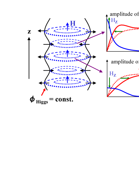
Figure 1: The illustration for the peristaltic mode of the vortex. The axial-symmetric oscillation perpendicular to the vortex line propagates with the excitation of the Higgs and photon fields. The waving solid line in the left side represents the surface where the amplitude of the Higgs field equals some constant value. The right hand side represents the amplitude of the Higgs and the magnetic fields in the cross section perpendicular to the vortex line. Through this process, the conserved total magnetic flux repeatedly contracts and relaxes.

Putting applications to the above examples in perspective, we will discuss the axial-symmetric radial excitation modes and their propagation along the vortex line. Hereafter, we will call this excitation mode peristaltic mode. The schematic picture of the peristaltic mode is shown in Fig.1. To discuss the peristaltic modes, we utilize the Abelian Higgs action which includes the Higgs and the photon fields. In terms of this action, the peristaltic modes are characterized by the Higgs and photon field fluctuations. In particular, the time-dependent photon fluctuations, which are sometimes neglected, play important roles on the corporative behavior with the Higgs field fluctuations. These fluctuations are regarded as the vibration of the vortex from the viewpoint that the vortex is the dynamical degrees of freedom in the system.

In this work, since we concentrate on the radial excitation modes, we simply neglect the effects of the boundary of the vortex edge, considering the vortex with the infinite length. The bending of the vortex is also neglected. We investigate both Type-I and Type-II vortices with not only usual $n$=1 but also $|n|\geq 2$ for the future applications to the non-equilibrium or multi-vortices systems where the giant vortices can appear as excited states. In the Type-I case, if the system contains only finite magnetic flux in contrast to the equilibrium case usually realized in the laboratory, these flux gather and become a $|n|\geq$ 2 giant vortex because Type-I vortices attract each other. On the other hand, in the Type-II case, the giant vortex is unstable and splits into the small vortices. In spite of this, when $\kappa^{2}$ is not too large, it is worth considering the vibration of the giant vortex because the gradient of the vortex-vortex interaction is small for the small separation of vortices jacob and we can expect that the fission process develops slowly.

The organization of this paper is as follows. In Sec.II we briefly review the treatments of the static profile of single vortex. In Sec.III we derive the effective action and the resulting equation of motion for the fluctuations around the vortex. The effects of the static vortex background on the fluctuations are emphasized. In Sec.IV we show the numerical results for the excitation modes of the $n$=1 vortex with 0.1$\leq$$\kappa^{2}$$\leq$1.0. Based on the classification with $\kappa^{2}$, we closely discuss their excitation energy, correlation energy between the Higgs and photon fields, spatial distribution of fluctuations, and the resulting magnetic flux behavior. It will be shown that, in the case of $\kappa^{2}\simeq$ 1/2, the interplay of the Higgs and the photon fields plays an essential role for the existence of the new-type discrete pole. We also discuss the excitation modes around $|n|\geq$ 2 vortices. In Sec.V we summarize this paper with the perspective for the future direction.

II Abelian Higgs model and the static Vortex

In this section, we briefly review the treatments of the static vortex in terms of Abelian Higgs model Nielsen . This type of action is very popular and has been used to describe cosmic string in the astrophysics vile , the color flux tube in QCD Suganuma2 , and so on. We use this Lorentz invariant action to investigate the properties of the vortex as a “pseudo-particle”.

For the finite temperature cases, one usually uses the phenomenological model with replacing the 2nd time-derivative in Abelian Higgs model with the 1st derivative although the microscopic foundation of this treatment is still not conclusive. The noise term is sometimes further added. These replacements change the equation of motion from the wave equation to the diffusive equation which respects the dissipation effects due to the thermal fluctuations. We will discuss the finite temperature case elsewhere.

II.1 The action and the field equation

Let us consider the ideal system which contains only one vortex with infinite length along the $z$-axis. Our purpose is to investigate the excitation mode of the vortex in such a system. We start with the following action with natural units ($c=\hbar=1$)

$$\bar{S}=\int d^{4}\bar{x}\bigg{\{}\mid(\bar{\partial}^{\mu}-ie\bar{A}^{\mu})\bar{\psi}\mid^{2}-\frac{1}{4}(\bar{\partial}^{\mu}\bar{A}^{\nu}-\bar{\partial}^{\nu}\bar{A}^{\mu})^{2}$$

$$-\lambda(\mid\bar{\psi}\mid^{2}-v^{2})^{2}\bigg{\}},$$ (1)

where $\bar{\psi}$ and $\bar{A}_{\mu}$ represent the Higgs field and photon field respectively. Here $e,\lambda,v$ are the effective gauge coupling constant, the strength of self-coupling, and the vacuum expectation value of the Higgs field, respectively. $\bar{x}^{\mu}$ denote space-time coordinates and $\bar{\partial}^{\mu}\equiv\frac{\partial}{\partial\bar{x}_{\mu}}$. Through this paper, we describe the variables in physical unit with bar. For later convenience, we rescale the fields and the coordinates to make them dimensionless quantities,

$$\psi=\bar{\psi}/v,\ A^{\mu}=\bar{A}^{\mu}/v,\ x^{\mu}=ev\bar{x}^{\mu}.$$ (2)

We also rewrite the action

$$S=e^{2}\bar{S}.$$ (3)

The energy relation between the physical and our rescaled unit can be obtained with noting the following relation,

$$\bar{S}=\int d\bar{t}\ \bar{L}\equiv\frac{1}{e^{2}}\int dt\ L=\int d\bar{t}\ \frac{v}{e}L.$$ (4)

Here $\bar{L}$ and $L$ are Lagrangian in physical and rescaled unit, respectively, and they are related as $\bar{L}=\frac{v}{e}L$. Similarly, we can obtain the energy and momentum in the physical unit with multiplying $v/e$ to our rescaled energy and momenta.

After these rewriting, the action reads

$$S=\int d^{4}x\bigg{\{}\mid(\partial^{\mu}-iA^{\mu})\psi\mid^{2}-\frac{1}{4}(\partial^{\mu}A^{\nu}-\partial^{\nu}A^{\mu})^{2}$$

$$-\kappa^{2}(\mid\psi\mid^{2}-1)^{2}\bigg{\}}.$$ (5)

Here we have introduced the GL parameter $\kappa^{2}=\lambda/e^{2}=\delta/\xi$, which is used to distinguish the Type-I ($\kappa<1/\sqrt{2}$ ) and Type-II ($\kappa>1/\sqrt{2}$ ) superconductors. The critical case of $\kappa=1/\sqrt{2}$ is called as the BPS case, which lies between Type-I and Type-II. As a remarkable fact in the BPS case, the photon mass $m_{A}$ and the Higgs mass $m_{\phi}$ coincide as $m_{A}=m_{\phi}$, because of $m_{A}=\sqrt{2}ev$ and $m_{\phi}=2\sqrt{\lambda}v$, i.e., $2\kappa^{2}=2\lambda/e^{2}=m_{\phi}^{2}/m_{A}^{2}$, which can be derived from the original action (II.1).

In this work, we will consider the system which is translation invariant in the $z$-direction and contains single vortex with infinite length along the $z$-axis. We also impose the axial-symmetry around the $z$-axis on the static solution. With cylindrical coordinates ($r,\theta,z$), we denote the complex field $\psi(x)$ in the polar-decomposed form

$$\psi(x)=\phi(t,r,\theta,z)e^{in\theta+i\chi(t,r,\theta,z)}\ \ (-\pi\leq\chi<\pi),$$ (6)

where $n$ is the topological number ($n$=0, $\pm$1, …) related to the phase of the Higgs field wave function around the $z$-axis. For single vortex with the topological number $n\in{\bf Z}$, the sign of $n$ is not relevant because of charge conjugation symmetry of the Abelian Higgs model, and therefore we have only to consider $n$=0, 1, …cases without loss of generality. Since the Abelian Higgs model has the U(1) local gauge symmetry, we have the degrees of freedom to choose the gauge. For the treatment of the vortex solution, the familiar gauge is the $A_{0}=0$ gauge. Instead, we adopt the gauge which eliminates the small amplitude of the phase,

$$\chi=0,$$ (7)

to simplify the equations of fluctuations in the later analysis. For $n$=0, this gauge fixing corresponds to the unitary gauge.

From the rotational symmetry and translational invariance along the $z$-direction, we adopt the following Ansatz for the static solutions

$$\psi(x) = \phi(r)e^{in\theta},$$

$$A^{\mu}(x) = (0,\ -A_{\theta}(r)\ {\rm sin}\theta,\ A_{\theta}(r)\ {\rm cos}\theta,\ 0\ ),$$ (8)

and the static electric and magnetic fields are obtained as

$${\bf E}(r)={\bf 0},\ \ {\bf H}(r)=(0,\ 0,\ \frac{1}{r}\frac{d}{dr}(rA_{\theta})\ ).$$ (9)

As seen soon later in Eq.(13) and (14), our gauge fixing and Ansatz for the static fields reproduce the same results for the static field solutions as those in usual $A_{0}=0$ gauge.

The total static energy of the system (in the rescaled unit) is obtained as $E=-S$ with putting the time derivative terms zero,

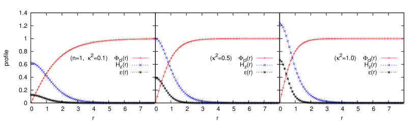
Figure 2: The profile for the Higgs field $\phi_{{\rm cl}}(r)$, the magnetic field $H_{z}(r)$ and static field energy ${\cal E}(r)$ for $\kappa^{2}$=0.1 (Type-I), $\kappa^{2}$=0.5 (BPS), $\kappa^{2}$=1.0 (Type-II) in the case of $n$=1 vortex.

$$E_{{\rm static}}=\int\!\!dzdr\ 2\pi r{\cal E}[\phi,A_{\theta}],$$ (10)

where

$${\cal E}[\phi,A_{\theta}]= \!\!\!(\partial_{z}\phi)^{2}+(\partial_{r}\phi)^{2}$$ (11)

$$\!\!\!+\frac{1}{2}(\partial_{z}A_{\theta})^{2}+\frac{1}{2}(\partial_{r}A_{\theta}+\frac{A_{\theta}}{r})^{2}$$

$$\!\!\!+\frac{(n-rA_{\theta})^{2}}{r^{2}}\phi^{2}+\kappa^{2}(\phi^{2}-1)^{2}.$$

(The full action and the energy functional are given in Appendix A.) Under the above circumstances, we consider the static vortex solutions $\phi(r)$ and $A_{\theta}(r)$ which minimize the static energy. From the variational principle

$$\frac{\delta E_{{\rm static}}}{\delta\phi(r)}=\frac{\delta E_{{\rm static}}}{\delta A_{\theta}(r)}=0,$$ (12)

and then the static field equations read

$$-\frac{1}{r}\frac{d}{dr}\big{(}r\frac{d\phi}{dr}\big{)}+\frac{(n-rA_{\theta})^{2}}{r^{2}}\phi+2\kappa^{2}\phi(\phi^{2}-1)=0,$$ (13)

$$\frac{d}{dr}\big{(}r\frac{dA_{\theta}}{dr}\big{)}-\frac{A_{\theta}}{r}+2(n-rA_{\theta})\phi^{2}=0.$$ (14)

Since we are interested in the vortex solution, we consider the boundary condition (B.C.) which is appropriate to describe the vortex at the center. For $r\rightarrow 0$,

$$\phi(r)\rightarrow{\rm const.}\times r^{n},\ A_{\theta}(r)\rightarrow{\rm const.}\times r,$$ (15)

and for $r\rightarrow\infty$,

$$\phi(r)\rightarrow 1+{\rm const.}\times r^{-\frac{1}{2}}e^{-2\kappa r},$$

$$A_{\theta}(r)\rightarrow\frac{n}{r}+{\rm const.}\times r^{-\frac{1}{2}}e^{-\sqrt{2}r}.$$ (16)

These boundary conditions are obtained by the asymptotic analysis of the static field equations which satisfy the following physical requirements to describe the vortex at the center: (I) at $r=0$ the vacuum expectation value of Higgs field takes zero. (II) the static field energy $U$ asymptotically approaches to the vacuum energy when $r\rightarrow\infty$. Note that the first condition represents the existence of the vortex at $r=0$ and the second one represents the magnetic fields are completely screened in the region far from the center of the vortex. The boundary conditions (15) and (II.1) also lead the quantization of the total magnetic flux $\Phi_{0}$,

$$\Phi_{0}\equiv\int_{0}^{\infty}\!\!\!dr\ 2\pi rH_{z}(r) = \int_{0}^{\infty}\!\!\!dr\ 2\pi\frac{d}{dr}(rA_{\theta}(r))$$ (17)

$$= 2\pi n.$$

($\Phi_{0}$ corresponds to $e\Phi$ in the physical unit.)

We can numerically solve the static field equations (13) and (14) with the boundary conditions (15) and (II.1) and obtain the static solutions $\phi^{{\rm cl}}(r)$ and $A^{{\rm cl}}_{\theta}(r)$ for the Higgs field $\phi(r)$ and the photon field $A_{\theta}(r)$. Fig.2 shows the static profiles of the Higgs field $\phi^{{\rm cl}}(r)$, the magnetic field $H^{{\rm cl}}(r)=\frac{1}{r}\frac{d}{dr}{(rA^{{\rm cl}}_{\theta})}$, and the resulting static energy distribution ${\cal E}(r)$ in the vortex with various $\kappa$.

II.2 The vortex mass and the classification of Type-I and Type-II superconductors

Using the distribution of the static field energy, we can calculate the vortex mass (with quantum number $n$) per unit length in the $z$-direction, i.e.,

$$M_{n}\equiv 2\pi\times\int_{0}^{\infty}\!\!\!dr\ r{\cal E}[\phi=\phi^{{\rm cl}},A_{\theta}=A^{{\rm cl}}].$$ (18)

Note that by definition of the action, the origin of energy is zero when the system has no vortex. The vortex mass is classified in the following way,

$$M_{n} < 2\pi n\ \ \ \ (\kappa^{2}<1/2\ ;{\rm Type-I}),$$ (19)

$$M_{n} = 2\pi n\ \ \ \ (\kappa^{2}=1/2\ ;{\rm BPS}),$$ (20)

$$M_{n} > 2\pi n\ \ \ \ (\kappa^{2}>1/2\ ;{\rm Type-II}).$$ (21)

These relations are analytically de vega ; bogo and numerically paul investigated. Fig.3 and 4 showed the numerically solved $\kappa^{2}$-dependence of $M_{n}/n$, the vortex mass divided by the topological number $n$, and we can see

$$M_{n}<nM_{1}\ \ \ (\kappa^{2}<1/2),$$

$$M_{n}>nM_{1}\ \ \ (\kappa^{2}>1/2).$$ (22)

These relations indicate that the interaction between vortices is attractive for $\kappa^{2}<$1/2, and repulsive for $\kappa^{2}>$1/2. These are confirmed by the studies of the vortex-vortex interaction analytically in large separation case kramer and numerically in arbitrary distance case jacob .

The qualitative understanding for the potential property is as follows. The attractive part of the potential comes from the reduction of the topological defect of the Higgs field condensate. This is because the total energy of the system decreases when the domain of the normal conducting state decreases. On the other hand, the repulsive part comes from the magnetic field interaction of the vortices. Then, in the case of $\kappa^{2}<$1/2 where the coherence length of the Higgs field exceeds the penetration depth of the magnetic field, the attractive part becomes larger than the repulsive part in the whole region, and the vortex-vortex potential becomes attractive. On the other hand, in the case of $\kappa^{2}>$1/2, the relation is reversed and the vortex-vortex potential becomes repulsive.

In the case of the vortex-anti-vortex case, the potential becomes attractive independently from $\kappa^{2}$ since the magnetic field interaction between the vortex and the anti-vortex becomes attractive in contrast to the vortex-vortex case, and there is no repulsive part in the potential.

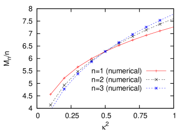
Figure 3: The plot for $\kappa^{2}$ dependence of the vortex mass divided by topological number $n$, $M_{n}/n$ for $n$=1, 2, 3 in the rescaled Abelian Higgs model in units of Eq.(2).

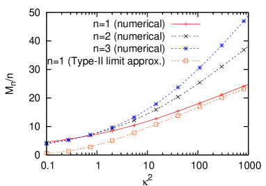
Figure 4: The plot for $\kappa^{2}$ dependence of the vortex mass divided by topological number $n$, $M_{n}/n$ for $n$=1, 2, 3 in the rescaled Abelian Higgs model in units of Eq.(2). The line with circle represents the mass of the $n$=1 vortex calculated with Type-II limit (large $\kappa^{2}$) approximation in abrikosov . The horizontal axis represents the log plot of $\kappa^{2}$ value in the much wider range than that in Fig. 3.

Although we consider the isolated vortex under the idealized situation from the beginning, it is worth mentioning under which situations single vortex appears referring to the potential properties explained above. In Type-I superconductor, the multi-vortices with total topological number $N$ transfer to the single, giant vortex with topological number $N$ due to their attractive interaction. After the successive fusion processes, the multi-vortices system transfers to the normal conducting state. For the finite size superconducting materials under the homogeneous magnetic fields and thermal equilibrium, such fusion processes lead the difficulty to observe the Type-I vortices because the magnetic fluxes successively invade from the interface between the normal and superconducting phase. Nevertheless, under the non-equilibrium situations or inhomogeneous magnetic fields concentrated on the small area, it is expected that the Type-I vortex or, more generally, the domain of the normal state in the superconductor can appear as a transient state in the process such as the dynamical evolution of the thermodynamic unstable state into the equilibrium state, i.e., the nucleation or spinodal decomposition processes frahm ; liu . From the viewpoint of the particle physics, an another interesting situation where Type-I vortex appears is the case where magnetic monopoles are immersed in superconductors and the isolated vortex emerges between the monopole and anti-monopole Nambu . In this case, no collapse with the other vortices occurs and Type-I vortex behaves as the stable object due to the topological charge conservation.

On the other hand, in Type-II superconductor, the giant vortex with topological charge $N$ fissions to the $N$ vortices with charge $n$=1 due to their repulsive nature jacob . This repulsive interaction prevents the vortices to coalescence and, under the thermal equilibrium, the $n$=1 vortices form some stable structure like the Abrikosov triangle lattice abrikosov . Then, in Type-II superconductor, the $n$=1 case is realistic in the thermodynamic equilibrium in contrast to Type-I case. However, when the system experience a certain quenching liu such as the rapid change of the temperature or density, the $n\geq 2$ vortex may be generated as the excited states. This is the reason why we also consider the Type-II giant vortex in the following. Although they are unstable against the fission into small vortices, when $\kappa^{2}$ is not too large, it may be interesting to consider the vibrations of the giant vortex because such vibrations can occur during the slow development of the fission process due to the small gradient of the vortex-vortex potential for the small separation of vortices jacob . Moreover, the study of the fluctuation modes of the $n\geq 2$ vortex may give some insight for the early stage of the evolution of the giant vortex into the multi-vortices.

III Axial-symmetric fluctuations

In this section, using the results of the previous section, we analyze axial-symmetric fluctuations in the system which has only one vortex in the background. In subsection A, using the static vortex profile, we derive the vortex-induced potential for the Higgs and photon field fluctuations, and the equation of motion. In subsection B, we closely discuss the potential feature to classify the type of the excitation modes.

III.1 Field equation for the fluctuations

We investigate the axial-symmetric fluctuations of the Higgs field and the related photon fields around the static vortex. We expand the fields with small amplitude fluctuations around the static field,

$$\phi(t,z,r)=\phi^{{\rm cl}}(r)+\varphi(t,z,r),$$

$$A_{\theta}(t,z,r)=A^{{\rm cl}}(r)+a_{\theta}(t,z,r).$$ (23)

Here we only consider the axial-symmetric fluctuations and we include $t,z$-dependence at this stage. It is important to notice that, with the Ansatz (II.1) for the static solution, all the other type of fluctuations such as fluctuations of $A_{0},A_{z},A_{r}$ and the $\theta$-dependent fluctuations are decoupled from the axial-symmetric fluctuations which we consider. Hence we can analyze the axial-symmetric fluctuations (III.1) independently from the other type of fluctuations and we drop off such fluctuation terms from the following Lagrangian. The complete form of the Lagrangian is given in the Appendix A.

Substituting Eq.(III.1) into Eq.(II.1) and using the static solution, the following expression for the axial-fluctuation part of Lagrangian can be derived as

$${\cal L}_{{\rm axial}}^{\chi=0}[\phi,A_{\theta}]={\cal L}_{{\rm axial}}^{{\rm cl}}+{\cal L}_{{\rm axial}}^{(2)}+{\cal L}_{{\rm axial}}^{(3)}+{\cal L}_{{\rm axial}}^{(4)}.$$ (24)

The first term ${\cal L}_{{\rm axial}}^{{\rm cl}}$ represents ${\cal L}_{{\rm axial}}^{{\rm cl}}\equiv{\cal L}_{{\rm axial}}^{\chi=0}[\phi_{{\rm cl}},A_{{\rm cl}}]$. The 1st order terms of fluctuations $\varphi$ and $a_{\theta}$ do not appear because we expand around the static solution. The 2nd, 3rd, and 4th order fluctuation terms take the following forms;

$${\cal L}_{{\rm axial}}^{(2)}\!\!\! = \!\!\!(\partial_{t}\varphi)^{2}-(\partial_{z}\varphi)^{2}-(\partial_{r}\varphi)^{2}$$ (25)

$$+\frac{1}{2}(\partial_{t}a_{\theta})^{2}-\frac{1}{2}(\partial_{z}a_{\theta})^{2}-\frac{1}{2}(\partial_{r}a_{\theta}+\frac{a_{\theta}}{r})^{2}$$

$$-V_{\varphi\varphi}\varphi^{2}-V_{\varphi a}\varphi a_{\theta}-V_{aa}a_{\theta}^{2},$$

$${\cal L}_{{\rm axial}}^{(3)}\!\!\! = \!\!\!-4\kappa^{2}\phi_{{\rm cl}}\varphi^{3}+2\bigg{[}\frac{n}{r}-A_{{\rm cl}}\bigg{]}\varphi^{2}a_{\theta}-2\phi_{{\rm cl}}\varphi a_{\theta}^{2},$$ (26)

$${\cal L}_{{\rm axial}}^{(4)}\!\!\! = \!\!\!-\kappa^{2}\varphi^{4}-\varphi^{2}a_{\theta}^{2}.$$ (27)

Here $V_{\varphi\varphi}$, $V_{aa}$, $V_{\varphi a}$ denote the vortex-induced potential, i.e., these interactions are induced by the static vortex configuration which can be regarded as the large amplitude background external field. $V_{\varphi\varphi}$ and $V_{aa}$ play roles as the single particle potential for $\varphi$ and $a_{\theta}$ respectively, and $V_{\varphi a}$ is the interaction which mixes the $\varphi$ and $a_{\theta}$. Hereafter, we will simply call these interactions “potentials”. The concrete forms of the potentials are

$$V_{\varphi\varphi}(r)=\bigg{[}\frac{n}{r}-A_{{\rm cl}}\bigg{]}^{2}+2\kappa^{2}(3\phi_{{\rm cl}}^{2}-1),$$

$$V_{\varphi a}(r)=-4\bigg{[}\frac{n}{r}-A_{{\rm cl}}\bigg{]}\phi_{{\rm cl}},$$

$$V_{aa}(r)=\phi_{{\rm cl}}^{2}.$$ (28)

To investigate the fluctuation spectrum, we solve the Euler-Lagrange equation for ${\cal L}^{(2)}$ neglecting the higher order fluctuations. The quantum loop corrections can be calculated using the Green’s functions constructed of bases which diagonalize ${\cal L}^{(2)}$. However, because of the inhomogeneous vortex-background, the Green’s functions are not functions of the distance between arbitrary two points, i.e., $G(x,x^{\prime})\neq G(x-x^{\prime})$, and the calculations of the loop corrections are not straightforward. In addition, higher order terms of the axial-symmetric fluctuations couple with the terms of the non-axial symmetric ones. We reserve the calculation of the loop corrections for the future work and, in this work, we safely neglect the quantum corrections constraining ourselves to the case where the perturbative expansion parameters $e^{2}$ and $e^{2}\kappa^{2}=\lambda$ are sufficiently small. (Recall that the perturbative corrections are calculated with expansion of $e^{i\bar{S}}=e^{ie^{2}S}$. See also Eq.(3).) These constraints are not so strict because the Higgs-photon coupling $e$ is usually small and we mainly consider $\kappa^{2}\sim 1/2$ cases, where $e^{2}\kappa^{2}=\lambda$ is also sufficiently small.

For later convenience to discuss the effect of the potential, we change the variables

$$\left(\begin{array}[]{c}\tilde{\varphi}(t,r,z)\\ \tilde{a}_{\theta}(t,r,z)\end{array}\right)=r^{-1/2}\left(\begin{array}[]{c}\varphi\\ a_{\theta}/\sqrt{2}\end{array}\right).$$ (33)

These changes of variables enable us to considerably simplify the equation of motion as will be seen. The Euler-Lagrange equation for 2nd order Lagrangian is obtained through the variation,

$$\frac{\delta}{\delta\tilde{\varphi}}\int dtdzdr2\pi r{\cal L}^{(2)}=\frac{\delta}{\delta\tilde{a}_{\theta}}\int dtdzdr2\pi r{\cal L}^{(2)}=0.$$ (34)

Then we obtain the following coupled equation

$$-\ (\ \partial_{t}^{2}-\partial_{z}^{2}\ )\left[\begin{array}[]{c}\tilde{\varphi}(t,z,r)\\ \tilde{a}_{\theta}(t,z,r)\end{array}\right] = \left[\begin{array}[]{cc}-\partial_{r}^{2}+\frac{4(n-A_{{\rm cl}})^{2}-1}{4r^{2}}+2\kappa^{2}(3\phi_{{\rm cl}}^{2}-1)&-\frac{2\sqrt{2}\phi_{{\rm cl}}(n-A_{{\rm cl}})}{r}\\ -\frac{2\sqrt{2}\phi_{{\rm cl}}(n-A_{{\rm cl}})}{r}&-\partial_{r}^{2}+\frac{3}{4r^{2}}+2\phi_{{\rm cl}}^{2}\end{array}\right]\left[\begin{array}[]{c}\tilde{\varphi}(t,z,r)\\ \tilde{a}_{\theta}(t,z,r)\end{array}\right]$$ (41)

$$\equiv \left[\begin{array}[]{cc}-\partial_{r}^{2}+V_{\alpha\alpha}(r)&V_{\alpha\beta}(r)\\ V_{\beta\alpha}(r)&-\partial_{r}^{2}+V_{\beta\beta}(r)\end{array}\right]\left[\begin{array}[]{c}\tilde{\varphi}(t,z,r)\\ \tilde{a}_{\theta}(t,z,r)\end{array}\right].$$ (46)

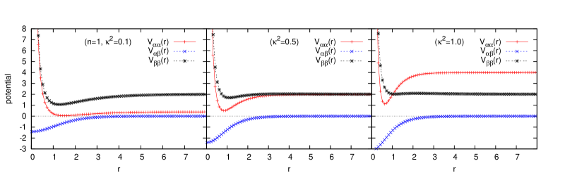
Figure 5: The plot of the vortex-induced potential $V_{\alpha\alpha}(r),V_{\alpha\beta}(r),V_{\beta\beta}(r)$ as the single particle potential for fluctuations $\alpha(r)$ and $\beta(r)$ around single vortex, defined in Eq.(51). The Ginzburg-Landau parameter takes $\kappa^{2}$=0.1, 0.5, 1.0, and the topological number takes $n$=1.

Here $V_{\alpha\beta}(r)=V_{\beta\alpha}(r)$ (This is the consequence of the change of the variables in Eq.(33)). Note that the $t,z$ dependence of $\tilde{\varphi}$ and $\tilde{a}_{\theta}$ is trivial because the background static vortex configuration is $t,z$-independent and $t,z$ dependence does not appear in the potential. Then the partial differential equation can be decoupled into the total differential equations for $t,z,r$, respectively.

The system has the translation invariance in both $z$-direction and time direction, and then the solution takes the following plane wave solution,

$$\left(\begin{array}[]{c}\tilde{\varphi}(t,r,z)\\ \tilde{a}_{\theta}(t,r,z)\end{array}\right)=e^{-i(\omega t-k_{z}z)}\left(\begin{array}[]{c}\alpha(r)\\ \beta(r)\end{array}\right).$$ (51)

Then the total differential equation in the radial direction for $\alpha(r)$ and $\beta(r)$ is obtained as

$$m_{j}^{2}\left[\begin{array}[]{c}\alpha_{j}\\ \beta_{j}\end{array}\right]=\left[\begin{array}[]{cc}-\frac{d^{2}}{dr^{2}}+V_{\alpha\alpha}(r)&V_{\alpha\beta}(r)\\ V_{\beta\alpha}(r)&-\frac{d^{2}}{dr^{2}}+V_{\beta\beta}(r)\end{array}\right]\left[\begin{array}[]{c}\alpha_{j}\\ \beta_{j}\end{array}\right],$$ (58)

(59)

where $m_{j}^{2}\equiv\omega_{j,k_{z}}^{2}-k_{z}^{2}$. Note that the Hermiticity of the matrix in the RHS in Eq.(59) ensures the real value of $m_{j}^{2}$ and our later analysis shows $m_{j}^{2}>0$, i.e., the stability of the static profile against the fluctuations. The root of the eigenvalue for the Eq.(59), $m_{j}$, plays a role of the mass for the propagating mode in the $z$-direction. The Hermiticity of Eq.(59) also enables us to take the functions $\alpha(r)$ and $\beta(r)$ real, and the orthonormal condition for the $\alpha(r)$ and $\beta(r)$ is expressed as

$$\int_{0}^{\infty}\!\!\!\!dr(\alpha_{j},\beta_{j})(\alpha_{k},\beta_{k})^{T} = \delta_{jk}\int_{0}^{\infty}\!\!\!\!dr\ [\alpha_{j}(r)^{2}+\beta_{j}(r)^{2}]$$ (60)

$$= \delta_{jk}.$$

Here we give a brief explanation for the qualitative picture for the excitation modes. The shape of the radial direction is given by $\alpha_{j}(r)$ and $\beta_{j}(r)$. This wave function propagates in the $z$-direction with the frequency $\omega_{j,k_{z}}$ and the wave vector $k_{z}$. Therefore the root of the eigenvalue $m_{j}^{2}$ of the radial wave functions $\alpha_{j}(r)$ and $\beta_{j}(r)$ play roles of the mass for the propagation in the $z$-direction. Then we call this type of new mode as the peristaltic mode of the vortex as illustrated in Fig.1.

III.2 The feature of the potential

We show in Fig.5 the single particle potentials $V_{\alpha\alpha}$, $V_{\alpha\beta}$ and $V_{\beta\beta}$ around the vortex for various values of $\kappa$. We can deduce the considerable information of the excitation modes from the examination of these potentials. To get the qualitative picture about the wave functions of fluctuations, it is convenient to divide the region of the coordinate space $r$ into three regions, central ($0\sim 0.5$), intermediate ($0.5\sim 4$), and asymptotic ($4\sim$) region in the rescaled Abelian Higgs model.

In the central region, when $r\rightarrow 0$, the asymptotic behavior of the potential is

$$V_{\alpha\alpha}\rightarrow\frac{4n^{2}-1}{4r^{2}},\ \ \ V_{\beta\beta}\rightarrow\frac{3}{4r^{2}},\$$

$$V_{\alpha\beta}=V_{\beta\alpha}\rightarrow({\rm negative\ const.})\times r^{n-1}\ .$$ (61)

From these asymptotic behavior, it is expected that the fluctuations $\alpha(r)$ and $\beta(r)$ around the vortex center are suppressed by the strong repulsive interaction proportional $1/r^{2}$ and their distributions are shifted to the outside.

On the other hand, in the intermediate region, the strong repulsive part of $V_{\alpha\alpha}$ and $V_{\beta\beta}$ becomes weak and the attractive pocket emerges. The mixing term $V_{\alpha\beta}$ also plays an important role to enhance the mixing between the Higgs and photon field fluctuations, or $\alpha$ and $\beta$. Since the $V_{\alpha\beta}$ always takes the negative value, the excitation energy is reduced when the relative sign of the $\alpha$ and $\beta$ fluctuations is positive. To avoid the confusion, we stress that the minus sign of $V_{\alpha\beta}$ does not mean attractive interaction. Even if $V_{\alpha\beta}$ takes the positive value, the energy is reduced when the relative sign of $\alpha$ and $\beta$ fluctuations is negative. This is also recognized from the fact that the replacement $(\alpha,\beta)\rightarrow(\alpha,-\beta)$ changes only the sign of the off-diagonal part of Eq.(59). In treatment up to the second order of the fluctuations, only the absolute value of $V_{\alpha\beta}$ is relevant to the mixing of $\alpha$ and $\beta$. All these features of the potentials $V_{\alpha\alpha},V_{\beta\beta},V_{\alpha\beta}$ make low energy modes of the fluctuations localized in the intermediate region.

Finally we discuss the asymptotic region. When $r\rightarrow\infty$, these potentials asymptotically behave as

$$V_{\alpha\alpha}\rightarrow 4\kappa^{2},\ \ \ V_{\beta\beta}\rightarrow 2,\ \ V_{\alpha\beta}=V_{\beta\alpha}\rightarrow 0.$$ (62)

Note that the asymptotic behaviors do not depend on the topological charge $n$. Since $V_{\alpha\beta}$ goes to zero, the correlation between $\alpha$ and $\beta$ vanishes and these fluctuations behave as independent modes. Then we have only to consider the one-particle problem in this region, i.e., we treat the asymptotic forms of Eq.(59) as

$$(-\frac{d^{2}}{dr^{2}}+4\kappa^{2})\alpha_{j}(r)\simeq m_{j}^{2}\alpha_{j}(r),$$ (63)

$$(-\frac{d^{2}}{dr^{2}}+2)\beta_{j}(r)\simeq m_{j}^{2}\beta_{j}(r).$$ (64)

The values $4\kappa^{2}$ and $2$ in the LHS play roles of the (square of) continuum thresholds of the $\alpha$ and $\beta$ respectively. These thresholds are equivalent to the masses of the fluctuations in the system with no vortex, i.e., $2\kappa$ corresponds to the mass of the Higgs field and $\sqrt{2}$ is the photon mass generated through the Anderson-Higgs mechanism ander ; higgs . Then, the threshold energy for the continuum states is expressed as

$$m_{{\rm th}}\equiv{\rm min}({2\kappa,\sqrt{2}}).$$ (65)

When $m_{j}^{2}$ is smaller (larger) than the thresholds, the fluctuations behave like bound (continuum) states.

It is also worth mentioning that $V_{\alpha\alpha}$ and $V_{\beta\beta}$ take the same value in the asymptotic region and the continuum thresholds are the same both for $\alpha$ and $\beta$ for the case of $\kappa^{2}$=1/2, where BPS saturation occurs. This note is sometimes useful to roughly classify the type of the fluctuation spectrum in the low-energy region in terms of the type of superconductor, as is explained below. It is expected that, for Type-I case ($\kappa^{2}<$1/2), the threshold for the Higgs field is lower than that for the photon field, and the Higgs field fluctuation dominates over the low energy physics. For Type-II case ($\kappa^{2}>$1/2), the relation is reversed, the photon field fluctuation dominates. We also expect that the collective properties induced by the mixing of the Higgs and photon field fluctuations are most pronounced when the BPS saturation occurs. This is because the strength of both fluctuations are the same order and they affect each other. In the next section, we will see the above mechanism is crucial to emerge the characteristic discrete pole around $\kappa^{2}=1/2$.

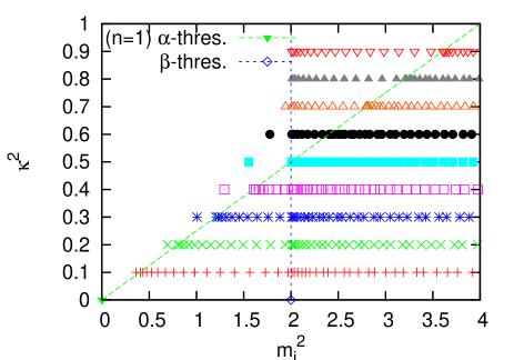
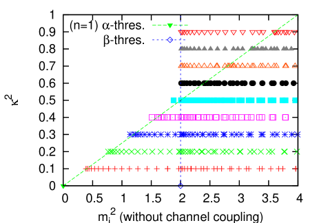
Figure 6: $\kappa^{2}$-dependence of $m_{j}^{2}$ for $n$=1 case and the square of thresholds for $\alpha$ and $\beta$ fields, 4$\kappa^{2}$ and 2, respectively. Around $\kappa^{2}$=$1/2$ (BPS value), as a collective mode of the Higgs and photon field fluctuations, there appear discrete poles in lower-energy region below (square of) the continuum threshold $m^{2}_{{\rm th}}={\rm min}(4\kappa^{2},2)$.

Figure 7: The same plot as Fig.7 except the replacement of $m_{j}^{2}$ with $m^{\prime 2}_{j}$, i.e., $m_{j}^{2}$ calculated in the case that the channel coupling between Higgs and photon field fluctuations is artificially dropped off. Without channel coupling, the bound-state with $\kappa^{2}\simeq 1/2$ becomes the shallow bound state due to the lack of the interplay between the Higgs and photon field fluctuations.

IV Appearance of the discrete pole as the peristaltic mode of the vortex

In this section, we summarize the numerical results in both Type-I and Type-II superconductors. The following results are obtained by solving the coupled channel equations (59) numerically with the lattice spacing 0.02 and the lattice size 40.0 in our rescaled unit. We impose the boundary condition on the wave function $\alpha(r)$ and $\beta(r)$ to be zero value at the box boundary. In the following, we consider $k_{z}=0$ case. The energy and radial wave functions shown in this section are translated into those in the general $k_{z}\neq 0$ case with the replacements $E=m_{j}\rightarrow(m_{j}^{2}+k_{z}^{2})^{1/2}$ and multiplying $e^{ik_{z}z}$ to the radial wave functions, respectively.

IV.1 Analysis for the excitation spectrum

In this subsection, we show the numerical results for $n$=1 case in both Type-I and Type-II superconductors. In Fig.7, the $\kappa^{2}$-dependence of $m_{j}^{2}$ for $n$=1 case and the thresholds for $\alpha$ and $\beta$ fields are plotted. Shown in Fig.7 are the same quantities as Fig.7, but without channel coupling, which is artificially dropped off.

With smaller $\kappa^{2}(<1/2)$, the threshold for $\alpha$ is shifted lower than threshold for $\beta$, and $\alpha$ can excite with smaller energy and the amplitude of $\alpha$ is enhanced compared to that of $\beta$ field. Then the lower excitation modes are mainly characterized by the $\alpha$ field fluctuation. Under the normalization condition (60), there appears a large excess of the amplitude of $\alpha$ field compared to that of $\beta$ field, and this mismatch between $\alpha$ and $\beta$ leads the suppression of the mixing effect. Then the properties of the lower excitations asymptotically approach to those calculated without channel coupling. The property of the discrete pole can be interpreted as the bound state of the static vortex and the fluctuating Higgs field.

On the other hand, with larger $\kappa^{2}(>1/2)$, the enhancement of the threshold energy for $\alpha$ leads the suppression of the $\alpha$ field excitation, and simultaneously enhances the $\beta$ field ratio in the lower excitation modes. Then the increasing of $\kappa^{2}$ value leads the reduction of the mixing correlation energy which is indispensable for the appearance of the discrete pole. Eventually, at $\kappa^{2}\simeq 0.8$, the discrete pole is buried in the continuum state spectrum of the fluctuating photon field and no discrete pole appears for $\kappa^{2}>0.8$. This indicates that such a pole is difficult to be identified in most Type-II superconductors.

Finally we consider the most interesting case, $\kappa^{2}\simeq 1/2$ case, i.e., near BPS saturation. In this case, the mixing effect becomes larger, and, as a result, the correlation between $\alpha$ and $\beta$ considerably lowers the excitation energy. This is clearly seen from the comparison of Fig.7 with Fig.7. In Table 1, we summarize the results for the lowest excitation energy $m_{j=0}$ and their relations to the threshold energy $m_{{\rm th}}={\rm min}\{2\kappa,\sqrt{2}\}$, the lowest excitation energy without channel coupling, $m^{\prime}_{0}$, and the energy differences among them. The quantity $m_{{\rm th}}-m_{0}$ represents the binding energy and specifies the spatial extension of the wave functions. The quantity $m^{\prime}_{0}-m_{0}$ is, roughly speaking, the correlation energy induced by the mixing effect between Higgs and photon field fluctuations. As expected, the maximum mixing correlation is realized in the BPS case ($\kappa^{2}$=1/2).

Table 1: $\kappa^{2}$ dependence of the various energy in the rescaled unit. The physical value can be obtained by multiplying $v/e$. $m_{{\rm th}}$, $m_{0}$, $m^{\prime}_{0}$ represent the threshold energy, the lowest excitation energy and the lowest excitation energy without the channel coupling, respectively. The negative sign of $m_{0}-m_{\rm th}$ indicates the bound state. The quantity $m_{0}-m^{\prime}_{0}$ roughly characterizes the correlation energy of the Higgs-photon field mixing.

$\kappa^{2}$	$m_{{\rm th}}$	$m_{0}$	$m_{0}-m_{{\rm th}}$	$m^{\prime}_{0}$	$m_{0}-m^{\prime}_{0}$
0.3	1.095	1.003	$-$0.092	1.068	$-$0.065
0.4	1.265	1.138	$-$0.127	1.229	$-$0.091
0.5	1.414	1.247	$-$0.167	1.371	$-$0.124
0.6	1.414	1.333	$-$0.081	1.414	$-$0.081
0.7	1.414	1.394	$-$0.020	1.414	$-$0.020

IV.2 The spatial behavior of the fluctuations and the character change of the excitation modes with $\kappa$

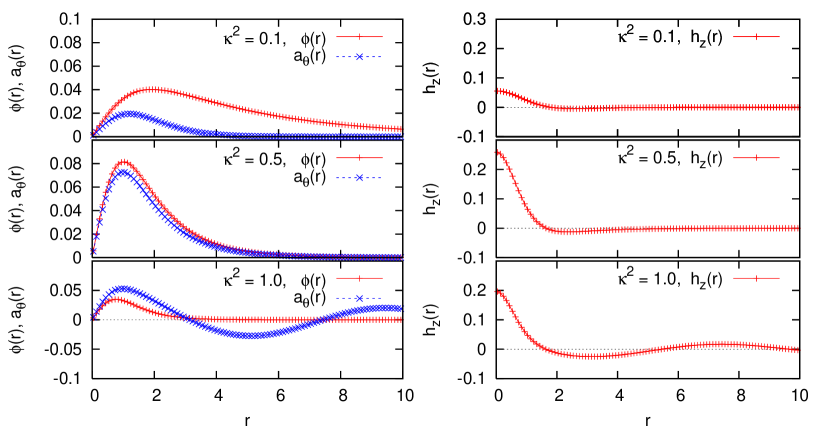
Figure 8: The behavior of the low-lying mode of Higgs field fluctuation $\varphi(r)\equiv r^{1/2}\alpha(r)$, the photon fluctuation $a_{\theta}(r)\equiv\sqrt{2}r^{1/2}\beta(r)$ and the magnetic field fluctuation $h_{z}(r)\equiv\frac{1}{r}\frac{d}{dr}(ra_{\theta})$ for $n$=1 vortex. For $\kappa^{2}=0.1,\ 0.5$ cases, we plot the lowest excitation mode with the radial mass $m_{0}$ smaller than the threshold $m_{{\rm th}}$. For $\kappa^{2}=1.0$ case, where the discrete pole does not appear, we plot the typical low-lying excitation mode with the radial mass $m_{j}$, satisfying $2<m_{j}^{2}<4\kappa^{2}$.

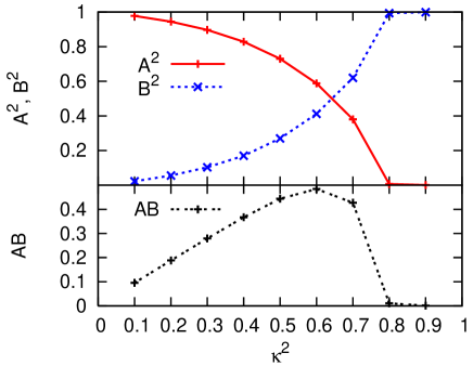
Figure 9: The $\kappa^{2}$-dependence of $A^{2}\equiv\int_{0}^{\infty}dr\ \alpha(r)^{2}$, $B^{2}\equiv\int_{0}^{\infty}dr\ \beta(r)^{2}$ and $A\cdot B\equiv\int_{0}^{\infty}dr\ \alpha(r)\beta(r)$ for the lowest excitation mode in the case of $n=1$.

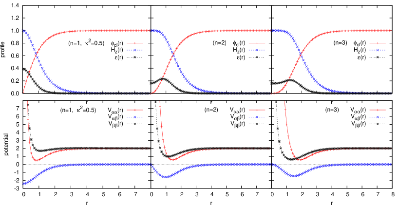
Figure 10: Shown in the upper panel are the profiles for $\phi_{{\rm cl}}(r)$, the magnetic field $H_{z}(r)$ and static field energy ${\cal E}(r)$ for $n$=1, 2, 3 vortices. The plots in the lower panel show the corresponding potential $V_{\alpha\alpha}(r),V_{\alpha\beta}(r)$ $V_{\beta\beta}(r)$ for the fluctuations $\alpha$ and $\beta$. $\kappa^{2}$ is fixed to the BPS value, i.e., $\kappa^{2}$=1/2.

The features explained above can be explicitly seen from the behavior of the radial wave function of the Higgs and the photon fields, i.e.,

$$\varphi(r)=r^{1/2}\alpha(r),\ a_{\theta}(r)=\sqrt{2}r^{1/2}\beta(r).$$ (66)

For the argument of the radial part, we hereafter drop off the trivial factor $e^{-i\omega t+k_{z}z}$ appearing in the relations (33) and (51). In fact, $\varphi(r)$ and $a_{\theta}(r)$ denote the radial part of the Higgs and the photon fluctuations in Eq.(III.1).

In Fig.8 we show the wave functions $\varphi(r)$ and $a_{\theta}(r)$ of the low-lying modes and the corresponding magnetic fluctuations

$$h_{z}(r)\equiv\frac{1}{r}\frac{d}{dr}(ra_{\theta}(r)),$$ (67)

for $\kappa^{2}$= 0.1, 0.5, 1.0. For $\kappa^{2}$ =0.1 and 0.5, we plot the lowest eigenfunction with radial mass smaller than the threshold $m_{{\rm th}}$. On the other hand, for $\kappa^{2}$ = 1.0, there is no discrete pole because the radial mass $m_{j}$ is larger than the threshold $m_{{\rm th}}=\sqrt{2}$, i.e., $m_{j}^{2}>2$. Then we plot the typical wave function of the low lying mode whose radial mass satisfying $2<m_{j}^{2}<4\kappa^{2}$.

The behavior of the fluctuation fields coincides to our previous expectations. For $\kappa^{2}$=0.1, the Higgs field fluctuation considerably exceeds to the photon fluctuation. Although both of fluctuation fields have the smaller excitation energy than the threshold $m_{{\rm th}}$ and this leads localization of them around the vortex core, the distribution of the Higgs field fluctuation spreads broader than that of the photon field fluctuation. This is because the lowest excitation energy $m_{0}$ is close to the threshold for the Higgs field fluctuations, $2\kappa$, and the lowest mode is characterized as the shallow bound-state between the static vortex and the Higgs field fluctuation.

When we change to the $\kappa^{2}$=0.5, the mixing correlation induces the corporative behavior of the Higgs and photon field fluctuations and enlarges the binding energy $m_{{\rm th}}-m_{0}$. As a result, the lowest excitation mode becomes the deeper bound-state, and then, the Higgs field localizes closer to the core, which affects the magnetic field vibration more strongly.

For $\kappa^{2}$=1.0, because of $2<m_{j}^{2}<4\kappa^{2}$ for low-lying modes, only Higgs field fluctuation is localized and the photon field $a_{\theta}(r)$ oscillates asymptotically ($r\rightarrow\infty$) as

$$a_{\theta}(r)\sim e^{ik_{r}r}/r^{1/2},$$ (68)

leading to the asymptotic behavior of the magnetic field $h_{z}(r)$ like

$$h_{z}(r)=\frac{1}{r}\frac{d}{dr}(ra_{\theta}(r))\sim e^{ik_{r}r}/r^{1/2}$$ (69)

with $k_{r}^{2}\equiv m_{j}^{2}-2$. (More precisely, $a_{\theta}(r)$ and $h_{z}(r)$ are expressed as the linear combinations of the ${\rm cos}(k_{r}r)/r^{1/2}$ and ${\rm sin}(k_{r}r)/r^{1/2}$ because $\varphi(r)$ and $a_{\theta}(r)$ are real functions.)

Here we comment on the total magnetic flux. In the static case, the total magnetic flux takes the quantized value $2\pi n$, as seen in Eq.(17). On the other hand, the photon fluctuation generally induces a time-dependent magnetic flux, whose proper time-average vanishes due to the factor $e^{-i\omega t}$. The contribution from the radial part of the magnetic field fluctuation is

$$\delta\Phi\equiv\int_{0}^{\infty}\!\!\!dr\ 2\pi rh_{z}(r) = \int_{0}^{\infty}\!\!\!dr\ 2\pi\frac{d}{dr}(ra_{\theta}(r))$$ (70)

$$= 2\pi\big{[}ra_{\theta}(r)\big{]}^{r=\infty}_{r=0}.$$

For $r\rightarrow 0$, $a_{\theta}(r)$ asymptotically approaches to zero. On the other hand, for $r\rightarrow\infty$,

$$ra_{\theta}(r)\rightarrow\left\{\begin{array}[]{l}Cr^{1/2}e^{-\sqrt{m_{{\rm th}}^{2}-m_{j}^{2}}r}\hskip 5.69046pt({\rm discrete\ pole}),\\ Dr^{1/2}e^{ik_{r}r}\hskip 36.98866pt({\rm continuum\ states}),\end{array}\right.$$ (73)

where $C$, $D$ represent some constants. Then, for the discrete pole, $\delta\Phi$ becomes zero and thus the total magnetic flux is conserved in the arbitrarily cross section perpendicular to the vortex line. In contrast, for the continuum states, the total magnetic flux becomes sensitive to the situation far from the vortex core because of the long tail behavior of $h_{z}(r)$. For the continuum state, the radial photon fluctuation $a_{\theta}(r)$ asymptotically behaves as a two-dimensional spherical wave in the homogeneous no-vortex vacuum, and hence its asymptotic part can be regarded as a non-vortex-origin fluctuation. In other words, the continuum states can be regarded as the vortex plus a “scattering wave”.

To discuss the character change of the excitation modes in wider range of $\kappa^{2}$, we define the functions

$$A^{2}\equiv\int_{0}^{\infty}dr\ \alpha(r)^{2},\ \ \ B^{2}\equiv\int_{0}^{\infty}dr\ \beta(r)^{2}.$$ (74)

Notice that $\int_{0}^{\infty}dr\ \big{[}\alpha(r)^{2}+\beta(r)^{2}\big{]}=1$ in the normalization condition. (See Eq.(60).) We also define the function to estimate the $\kappa^{2}$-dependence of the collective properties and their mixing ratio for the lowest eigenmode. One of the good indicators to estimate the degree of the collective nature is the function

$$A\cdot B\equiv\int_{0}^{\infty}dr\ \alpha(r)\beta(r).$$ (75)

When the oscillation is sympathetic, this integral takes the large value. In Fig.9 we plot the behavior of the functions $A^{2}$, $B^{2}$ and $A\cdot B$ for various $\kappa^{2}$. As expected, the ration of $\alpha(r)$, or Higgs field decreases compared to that of $\beta(r)$, or photon fluctuation with increasing $\kappa^{2}$ because the threshold for the Higgs field fluctuation increases. Eventually, around $\kappa^{2}\simeq 0.8$, the discrete pole buries in the continuum, and the lowest mode becomes the continuum state of the photon field. At the same time, the correlation between the Higgs and photon field fluctuations becomes very small, as seen in the lower panel in Fig.9.

IV.3 The peristaltic modes for $n\geq 2$ cases

In this subsection, we show the results for the peristaltic modes of the $n\geq 2$ vortex, which is realistic in the case of $\kappa^{2}\leq 1/2$. We emphasize the difference of the static vortex between $n$=1 vortex and $n$=2, 3 vortex, and then discuss their effects on the potential behavior and the resulting excitation spectrum. In this subsection, when we argue $n$-dependence of the classical profile and the potential, $\kappa^{2}$ value is fixed to BPS value, i.e., $\kappa^{2}$=1/2.

Shown in Fig.10 are the $n$=1, 2, 3 static vortex profiles and the corresponding vortex-induced potentials $V_{\alpha\alpha}$, $V_{\beta\beta}$, $V_{\alpha\beta}$ for the fluctuations $\alpha(r)$ and $\beta(r)$, respectively. Here we qualitatively explain the changes of the static vortex profiles in terms of $n$. Since the total penetrating flux of the magnetic field is proportional to the topological number $n$, the magnetic field around the vortex core increases with increasing $n$. Then the enlarged magnetic flux pushes the Higgs field outward or reduce the expectation value of the Higgs field. Roughly, this process spreads the normal phase region near the vortex core and leads the outward shift of the interface between normal and superconducting phase. According to the outward shift of the surface region, where the kinetic energy of the Higgs field is enhanced, the maximum of the local energy density also shifts outward, as seen in the upper panel of Fig.10.

Next we present the qualitative explanation for the single particle potential for the fluctuation fields. First we give the explanation for the change of $V_{\alpha\alpha}$ for the Higgs field fluctuation. Since the area of the magnetic flux is spread with increasing $n$, the intersection surface of the static magnetic and the Higgs fields moves outward. This leads the outward shift of the potential $V_{\alpha\alpha}$.

The changes of $V_{\beta\beta}$ can be interpreted in somewhat indirect way as follows. The fact read off from Fig. 10 is the depth enhancement of the attractive pocket in $V_{\beta\beta}$ with increasing $n$. This enables the photon field fluctuations to enhance and localize around the surface region more easily for larger $n$ cases. The localization of the photon field fluctuation means somewhat rapid spatial change of the wave function $a_{\theta}(r)$, and leads a large fluctuation of the magnetic field $h_{z}(r)=\frac{1}{r}\frac{d}{dr}(ra_{\theta})$. Then we can say that the depth enhancement of the attractive pocket in $V_{\beta\beta}$ for large $n$ leads the large fluctuation of the magnetic field. The large magnetic fluctuation reflects the reduction of the Higgs field condensate or the weakened Meissner effect. In fact, the depth enhancement of the attractive pocket is closely related to the outward shift of the static Higgs field distribution.

Finally we comment on the potential $V_{\alpha\beta}$, which induces the mixing correlation between the Higgs and the photon field fluctuations. As seen in Fig. 10, with increasing $n$, the maximum of $|V_{\alpha\beta}|$ shifts outward. The physical meaning of the change in this potential is naturally explained as the outward shift of the interface between the static Higgs field and magnetic field because, at the interface, the fluctuations of the Higgs and photon field can frequently interplay.

With increasing $n$, the resulting changes in the static configurations and the vortex-induced potential lead the change of the excitation energy of the peristaltic modes. Now we see the excitation spectra of the giant vortex ($n=2,3$) and their dependence on the $\kappa^{2}$ value. The numerical results for $n=2,3$ cases are shown in Figs. 12, 12, respectively. For larger $n$, the excitation energy for the lowest mode becomes much smaller as expected from the arguments in the previous paragraphs. As a consequence of the depth enhancement of the attractive pocket in $V_{\beta\beta}$, the discrete pole appears up to considerably large $\kappa^{2}$ value in the Type-II region.

In such large $\kappa^{2}(>1/2)$ cases, of course, the fission processes of the giant vortex to many $n$=1 vortices become important. According to the analysis for the instability of the static vortex bogo ; gustafson and the interaction between two vortices jacob , there exists no potential barrier for the fission from single Type-II giant vortex to many $n$=1 vortices and the giant vortex can fission through the non-axial symmetric modes. However, in spite of this observation, we have a possibility that axial-symmetric discrete poles play important roles if the lifetime (decay width) of the giant vortex is very large compared to the typical time scale (excitation energy) of the axial-symmetric fluctuations. The decay rate can be calculated through the analysis for the non-axial-symmetric modes and the fluctuations of $A_{0},A_{r}$, which are not considered in this work. We expect that, for $\kappa^{2}$ not so far beyond the BPS value, $\kappa^{2}=1/2$, the lifetime is large because the force to break up the giant vortex is small. Then, if the lifetime is confirmed to be large enough, we can immediately apply our results without further consideration about the correlation between the axial-symmetric and the other modes because these modes behave independently as far as the distortion is sufficiently small, as noticed in Sec.IIIA.

On the other hand, for $\kappa^{2}\leq 1/2$ cases, since the giant vortex is stable and the axial-symmetric modes are independent from the other modes not considered in this work, the strong bound-state-like modes more easily appear than the case for $\kappa^{2}>1/2$ because of non-existence of the fission processes. In addition, according to the negative surface tension, vortex with $\kappa^{2}\leq 1/2$ tends to reduce the surface area and then the axial-symmetric fluctuation becomes increasingly prominent with smaller $\kappa^{2}$. Therefore, we expect that the discrete pole shown in this section shares the considerable relevance to the low-energy behavior of the giant vortex with $\kappa^{2}\leq 1/2$.

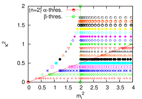
Figure 11: $\kappa^{2}$-dependence of $m_{j}^{2}$ for $n$=2 case and the square of thresholds for $\alpha$ and $\beta$ fields, $4\kappa^{2}$ and $2$, respectively. The excitation energy is considerably lowered than that in $n$=1 case and the discrete pole appears up to considerably large $\kappa^{2}$.

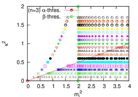
Figure 12: The same plot as Fig.12 except the replacement of the topological number $n$ from $n$=2 to $n$=3. The thresholds for $\alpha$ and $\beta$ are unchanged.

V Summary and Concluding Remarks

In this paper, as a new-type mode beyond the stringy one, we have studied the axial-symmetric peristaltic modes of the vortex, peculiar to the extension of the flux-tube. We have investigated the peristaltic modes both in Type-I and Type-II superconductors for $n=$1, 2, 3 and $\kappa^{2}=0.1\sim 1.0$. We have treated single vortex in the situation where Type-I vortex can be realized without collapses with the other vortices and behaves as the stable object.

Here we summarize our main results about the fluctuation modes. With $\kappa^{2}<1/2$, the lowest excitation modes are characterized by the Higgs field fluctuation binding with the static vortex. On the other hand, with $\kappa^{2}>1/2$, the mass of the Higgs field fluctuation becomes heavier and the photon fluctuation modes are relevant. For $\kappa^{2}=1/2$ (BPS cases), there appears the characteristic discrete pole. In this case, the Higgs and the photon field fluctuations have the same masses, and then both fluctuations play important roles and their corporative behavior makes the lowest excitation softer one. This mechanism is the main origin of the characteristic discrete pole. Since the energy separation between this discrete pole and the continuum threshold is large around $\kappa^{2}\simeq 1/2$, the peristaltic mode may appear most clearly in the superconductor with $\kappa^{2}\simeq 1/2$.

We have also investigated the fluctuation modes of the giant vortex with the topological number $n\geq 2$. It is found that, with larger $n$, the photon field fluctuation becomes more important for the lowest eigenmode because the distribution of the static Higgs field is shifted outward and the photon fluctuation can excite easily around the core. We expect that, in $\kappa^{2}\leq 1/2$ cases, the axial-symmetric excitation mode with the bound-state-like pole plays an important role in the low-energy dynamics of the vortex. On the other hand, for $\kappa^{2}>1/2$ cases, although the equations for axial-symmetric excitation modes are decoupled from those of the other modes, it is necessarily not only to investigate axial-symmetric modes but also to consider whether these excitation modes can be realized or not during the lifetime of the giant vortex. To estimate the lifetime, we have to treat the non-axial-symmetric modes and the fluctuations of $A_{0},A_{r}$, which drive the fission of the single giant vortex to many $n$=1 vortices. We expect that, for $\kappa^{2}$ value not so far from the BPS value, $\kappa^{2}$=1/2, the life time is long enough and we can explore the possibility of the appearance of the discrete pole.

Finally, we end with a future perspective toward the further investigation for the dynamics of the vortices (or color-electric flux tubes) regarding them as dynamical degrees of freedom.

Although we restrict ourselves to the axial-symmetric static vortex profile and fluctuations of $\phi$ and $A_{\theta}$, we will investigate the more general cases without using the axial-symmetric Ansatz for the static profile and classify the large class of the fluctuation modes, i.e., ($\phi$, $A_{0}$, $A_{\theta}$, $A_{r}$) in $\chi=0$ gauge, or equivalently, ($\phi$, $\chi$, $A_{\theta}$, $A_{r}$) in $A_{0}=0$ gauge, which are not fully considered in this work. For this purposes, we will calculate the static vortex profile and excitation spectrum of the fluctuations in two-dimensional analysis in near future.

For Type-I case, we expect that, in low energy, the relevant excitation mode around single vortex is axial-symmetric since the Type-I vortex tends to reduce the surface area owing to the positive surface tension. Also from the point of view on the kinetic energy, the axial-symmetric excitation is favorable. On the other hand, the arguments for the Type-II case are more subtle. Because Type-II vortex tends to increase the surface area according to the negative surface tension, it may be important to compare the surface energy to the kinetic energy of the distortion.

For $n\geq 2$ giant vortices, interesting subjects are remained. One of them is the calculation of the lifetime of single giant vortex for $\kappa^{2}>1/2$ and the comparison to the excitation modes considered in this work. The lifetime of the giant vortex is closely related to the dynamics of the multi-vortices in non-equilibrium systems. As well as the information for the vortex-vortex potential, the information for the lifetime of single giant vortex may provide the good building block to understand the interesting but complicated phenomena such as the transition of the system from the thermodynamically unstable state to the stable one. In connection with them, we are also interested in the fluctuations between multi-vortices and their evolution through the vortex-vortex scattering myers . As a successive study, we would like to investigate the results of the full two-dimensional analysis for excitation modes of the vortex in both single vortex and the multi-vortices system kst .

In application to QCD, the dynamics of the color-electric flux-tubes, or gluonic excitations as nonperturbative modes are also important to discuss the hadrons, which are composed of quarks and color vortex between quarks. In particular, the analysis for the multi-color-flux-tube system can give an good insight to understand the color confinement-deconfinement transition in QCD, and properties of the hot and dense matter of hadrons or quarks. It is also interesting to consider heavy ion collisions and the successive occuring expansion of the hot quark matter in close analogy with the evolution of the early Universe. The distribution of the topological defects may affect collective properties of quark gluon plasma and the resulting particle productions.

In this work, we have studied the dynamics of single vortex as one example of the dynamics of the topological objects. The treatments of topological objects as essential degrees of freedom are quite general and important to understand the crucial aspects of the nonlinear field theory, which sometimes can not be reached with the perturbative treatments for the nonlinear terms. We would like to extend our analysis to the other topological objects such as color flux-tubes, instantons, magnetic monopoles in gauge theories, or branes in the string theory nitta , and their many-body dynamics.

Note added: After this work is completed, we notice a similar study using a different gauge where ghosts appear GH95 . Their numerical result on the physical modes is consistent with ours.

Appendix A The decoupling of the axial-symmetric fluctuation modes

We give the complete form of the action in the cylindrical coordinates ($r,\theta,z$). We use the polar-decomposition of Eq.(6) for the Higgs field

$$\psi(x)=\phi(t,r,\theta,z)e^{in\theta+i\chi(t,r,\theta,z)}\ \ (-\pi\leq\chi<\pi),$$ (76)

and fix the gauge to $\chi=0$. Then we obtain the action as

$$S^{\chi=0}=\int\!\!dtdrd\theta dz\ r{\cal L}^{\chi=0},$$ (77)

where

$${\cal L}^{\chi=0} = (\partial_{t}\phi)^{2}-(\partial_{r}\phi)^{2}-\frac{1}{r^{2}}(\partial_{\theta}\phi)^{2}-(\partial_{z}\phi)^{2}-\kappa^{2}(\phi^{2}-1)^{2}-\frac{(n-rA_{\theta})^{2}}{r^{2}}\phi^{2}+(A_{0}^{2}-A_{r}^{2}-A_{z}^{2})\phi^{2}$$ (78)

$$+\frac{1}{2}[E_{r}^{2}+E_{\theta}^{2}+E_{z}^{2}-B_{r}^{2}-B_{\theta}^{2}-B_{z}^{2}].$$

Here the electric and magnetic fields are described as

$$E_{r}=\partial_{t}A_{r}-\partial_{r}A_{0},\ \ E_{\theta}=\partial_{t}A_{\theta}-\frac{1}{r}\partial_{\theta}A_{0},\ \ E_{z}=\partial_{t}A_{z}-\partial_{z}A_{0},$$ (79)

$$B_{r}=\frac{1}{r}\partial_{\theta}A_{z}-\partial_{z}A_{\theta},\ \ B_{\theta}=\partial_{z}A_{r}-\partial_{r}A_{z},\ \ B_{z}=\frac{1}{r}\partial_{\theta}(rA_{r})-\frac{1}{r}\partial_{\theta}A_{r}.$$ (80)

We decompose the field into the static part and fluctuation part,

$$\phi(t,r,\theta,z)=\phi^{{\rm cl}}(r,\theta,z)+\varphi(t,r,\theta,z),$$

$$A_{j}(t,r,\theta,z)=A^{{\rm cl}}_{j}(r,\theta,z)+a_{j}(t,r,\theta,z),$$ (81)

where $j=(0,r,\theta,z)$. For the static part, we impose the Ansatz (II.1), or equivalently,

$$\phi^{{\rm cl}}(r,\theta,z)=\phi^{{\rm cl}}(r),\ \ A^{{\rm cl}}_{\theta}(r,\theta,z)=A^{{\rm cl}}_{\theta}(r),\ \ A^{{\rm cl}}_{0}=A^{{\rm cl}}_{r}=A^{{\rm cl}}_{z}=0.$$ (82)

Putting these forms into the Lagrangian (78), we obtain

$${\cal L}^{\chi=0}[\phi,A_{\theta}]={\cal L}^{{\rm cl}}+{\cal L}^{(2)}+{\cal L}^{(3)}+{\cal L}^{(4)},$$ (83)

where

$${\cal L}^{{\rm cl}}=-(\partial_{r}\phi^{{\rm cl}})^{2}-\frac{1}{2}(\partial_{r}A^{{\rm cl}}_{\theta}+\frac{A^{{\rm cl}}_{\theta}}{r})^{2}-\frac{(n-rA^{{\rm cl}}_{\theta})^{2}}{r^{2}}\phi_{{\rm cl}}^{2}-\kappa^{2}(\phi_{{\rm cl}}^{2}-1)^{2},$$ (84)

$${\cal L}^{(2)}=(\partial_{t}\varphi)^{2}-(\partial_{r}\varphi)^{2}-\frac{1}{r^{2}}(\partial_{\theta}\varphi)^{2}-(\partial_{z}\varphi)^{2}-2\kappa^{2}(3\phi_{{\rm cl}}^{2}-1)^{2}\varphi^{2}-\frac{(n-rA^{{\rm cl}}_{\theta})^{2}}{r^{2}}\varphi^{2}$$

$$\ \ \ \ \ \ \ \ +\frac{1}{2}[e_{r}^{2}+e_{\theta}^{2}+e_{z}^{2}-b_{r}^{2}-b_{\theta}^{2}-b_{z}^{2}]+\phi_{{\rm cl}}^{2}(a_{0}^{2}-a_{r}^{2}-a_{\theta}^{2}-a_{z}^{2})+\frac{4\phi_{\rm cl}(n-rA^{{\rm cl}}_{\theta})}{r}\varphi a_{\theta},$$ (85)

$${\cal L}^{(3)}=-4\kappa^{2}\phi^{{\rm cl}}\varphi^{3}+\frac{2(n-rA^{{\rm cl}}_{\theta})}{r}\varphi^{2}a_{\theta}+2\phi^{{\rm cl}}\varphi(a_{0}^{2}-a_{r}^{2}-a_{\theta}^{2}-a_{z}^{2}),$$ (86)

$${\cal L}^{(4)}=\varphi^{2}(a_{0}^{2}-a_{r}^{2}-a_{\theta}^{2}-a_{z}^{2})-\kappa^{2}\varphi^{4}.$$ (87)

The Lagrangian for the static part, i.e., ${\cal L^{{\rm cl}}}$ is related to static energy (11) as ${\cal E}=-{\cal L}^{{\rm cl}}$. The fluctuations of the electric and magnetic fields, i.e., $(e_{r},e_{\theta},e_{z})$ and $(b_{r},b_{\theta},b_{z})$ are expressed as the Eq.(79) with the substitution $A_{j}\rightarrow a_{j}$. The linearized Euler-Lagrange equations for the fluctuations $\varphi,a_{\theta},a_{0},a_{r},a_{z}$ are obtained as

$$\!\!\!\!\!\!\!\!\!\!\!\!\!\!\!\!\!\bigg{[}\frac{\partial^{2}}{\partial t^{2}}-\frac{1}{r}\frac{\partial}{\partial r}\big{(}r\frac{\partial}{\partial r}\big{)}-\frac{1}{r^{2}}\frac{\partial^{2}}{\partial\theta^{2}}-\frac{\partial^{2}}{\partial z^{2}}\bigg{]}\varphi\!\!\!\! =-\bigg{[}\frac{(n-rA^{{\rm cl}}_{\theta})^{2}}{r^{2}}+2\kappa^{2}(3\phi^{{\rm cl}}-1)^{2}\bigg{]}\varphi+\frac{2\phi^{{\rm cl}}(n-rA_{\theta}^{{\rm cl}})}{r}a_{\theta},$$ (88)

$$\!\!\!\!\!\!\!\!\!\!\!\!\!\!\!\!\!\bigg{[}\frac{\partial^{2}}{\partial t^{2}}-\frac{1}{r}\frac{\partial}{\partial r}\big{(}r\frac{\partial}{\partial r}\big{)}-\frac{\partial^{2}}{\partial z^{2}}\bigg{]}a_{\theta}\!\!\!\!\!\! =-\bigg{[}\frac{1}{r^{2}}+2\phi_{{\rm cl}}^{2}\bigg{]}a_{\theta}-\frac{4\phi^{{\rm cl}}(n-rA^{{\rm cl}}_{\theta})^{2}}{r^{2}}\varphi+\frac{1}{r}\frac{\partial}{\partial\theta}\bigg{[}\frac{\partial a_{0}}{\partial t}-\frac{1}{r}\frac{\partial(ra_{r})}{\partial r}-\frac{\partial a_{z}}{\partial z}\bigg{]},$$ (89)

$$\!\!\!\!\!\!\!\!\!\!\!\!\!\!\!\!\!\bigg{[}-\frac{1}{r}\frac{\partial}{\partial r}\big{(}r\frac{\partial}{\partial r}\big{)}-\frac{1}{r^{2}}\frac{\partial^{2}}{\partial\theta^{2}}-\frac{\partial^{2}}{\partial z^{2}}\bigg{]}a_{0}\!\!\!\!\!\! =-2\phi_{\rm cl}^{2}a_{0}-\frac{\partial}{\partial t}\bigg{[}\frac{1}{r^{2}}\frac{\partial a_{\theta}}{\partial\theta}+\frac{1}{r}\frac{\partial(ra_{r})}{\partial r}+\frac{\partial a_{z}}{\partial z}\bigg{]},$$ (90)

$$\!\!\!\!\!\!\!\!\!\!\!\!\!\!\!\!\bigg{[}\frac{\partial^{2}}{\partial t^{2}}-\frac{1}{r^{2}}\frac{\partial^{2}}{\partial\theta^{2}}-\frac{\partial^{2}}{\partial z^{2}}\bigg{]}a_{r}\!\!\!\!\!\! =-2\phi_{{\rm cl}}^{2}a_{r}-\frac{2}{r^{2}}\frac{\partial a_{\theta}}{\partial\theta}+\frac{\partial}{\partial r}\bigg{[}\frac{\partial a_{0}}{\partial t}-\frac{1}{r}\frac{\partial a_{\theta}}{\partial\theta}-\frac{\partial a_{z}}{\partial z}\bigg{]},$$ (91)

$$\!\!\!\!\!\!\!\!\!\!\!\!\!\!\!\!\bigg{[}\frac{\partial^{2}}{\partial t^{2}}-\frac{1}{r}\frac{\partial}{\partial r}\big{(}r\frac{\partial}{\partial r}\big{)}-\frac{1}{r^{2}}\frac{\partial^{2}}{\partial\theta^{2}}\bigg{]}a_{z}\!\!\!\!\!\! =-2\phi_{{\rm cl}}^{2}a_{z}-\frac{\partial}{\partial z}\bigg{[}\frac{\partial a_{0}}{\partial t}-\frac{1}{r}\frac{\partial a_{\theta}}{\partial\theta}-\frac{1}{r}\frac{\partial(ra_{r})}{\partial r}\bigg{]}.$$ (92)

It is important to notice that we can decouple the equations for the axial-symmetric fluctuations of $\varphi$ and $a_{\theta}$ expanding the fluctuation modes with the Legendre polynomial. If we restrict ourselves to the $l=0$ modes analysis, we can neglect angular-derivative terms in Eq.(88)-(92). Therefore, we can treat the fluctuations $\varphi$ and $a_{\theta}$ independently from fluctuations $a_{0},a_{r},a_{z}$, because $\varphi$ and $a_{\theta}$ are related to $a_{0},a_{r},a_{z}$ only through the angular-derivative terms. As a result, to investigate the axial-symmetric fluctuations of $\varphi$ and $a_{\theta}$, we have only to treat the Lagrangian (25) as mentioned in Sec.IIIA.

References

- (1) A. A. Abrikosov, Soviet Phys. JETP 5, 1174 (1957).
- (2) P. A. M. Dirac, Proc. Roy. Soc. A133, 60 (1934),
- (3) G. ’t Hooft, Nucl. Phys. B79, 276 (1974), A. M. Polyakov, JETP Lett 20, 194 (1974).
- (4) A. A. Belavin, A. M. Polyakov, A. S. Schwartz, and Y. S. Tyupkin, Phys. Lett. 59B, 85 (1975).
- (5) R. Rajaraman, Solitons and Instantons, (North-Holland, 1987).
- (6) N. Manton and P. Sutcliffe, Topological Solitons, (Cambridge University Press, Cambridge, 2004) and references therein.
- (7) H. B. Nielsen and P. Olesen, Nucl. Phys. B61, 45 (1973).
- (8) Y. Nambu, Phys. Rev. D10, 4262 (1974).
- (9) G. ’t Hooft, Nucl. Phys. B190, 455 (1981).
- (10) S. Mandelstam, Phys. Rept. C23, 245 (1976).
- (11) Color Confinement and Hadrons in Quantum Chromodynamics edited by H. Suganuma, N. Ishii, M. Oka, H. Enyo, T. Hatsuda, T. Kunihiro, and K. Yazaki (World Scientific, Singapore, 2004)
- (12) H. J. Rothe, Lattice Gauge Theories: An Introduction, 3rd edition (World Scientific, Singapore, 2005)
- (13) M. Creutz, Phys. Rev. Lett. 43, 553 (1979); 43, 890 (1979); Phys. Rev. D 21, 2308 (1980).
- (14) T.T. Takahashi, H. Matsufuru, Y. Nemoto, and H. Suganuma, Phys. Rev. Lett. 86, 18 (2001); T.T. Takahashi, H. Suganuma, Y. Nemoto, and H. Matsufuru, Phys. Rev. D 65, 114509 (2002).
- (15) H. Ichie, V. Bornyakov, T. Streuer, and G. Schierholz, Nucl. Phys. A721, C899 (2003).
- (16) A. Vilenkin and E. P. S. Shellard, Cosmic Strings and Other Topological Defects, (Cambiridge University Press, Cambridge, 1994) and references therein.
- (17) T. W. B. Kibble, J. Phys. A 9, 1387 (1976).
- (18) W. H. Zurek, Nature (London) 317, 505 (1985); Phys. Rep. 276, 177 (1996).
- (19) See, for example, M. Tinkham, Introduction to Superconductivity (Krieger, Malabar, 1985).
- (20) M. Hindmarsh and A. Rajantie, Phys. Rev. Lett. 85, 4660 (2000).
- (21) G. J. Stephens, L. M. A. Bettencourt, and W. H. Zurek, Phys. Rev. Lett. 88, 137004 (2002).
- (22) For instance, J. Polchinski, String Theory, (Cambridge University Press, Cambridge, 1998).
- (23) K. Nawa, H. Suganuma and T. Kojo, Phys. Rev. D85, 086003 (2007), and its references.
- (24) M. Luscher, G. Munster and P. Weisz, Nucl. Phys. B180, 1 (1981).
- (25) P. Orland, Nucl. Phys. B428, 221 (1994) and its references.
- (26) E.T. Akhmedov, M.N. Chernodub, M.I. Polikarpov and M.A. Zubkov, Phys. Rev. D53, 2087 (1996) and its references.
- (27) E. B. Bogomol’nyi, Sov. J. Nucl. Phys. 24, 449 (1976).
- (28) M. K. Prasad and C. M. Sommerfield, Phys. Rev. Lett. 35, 760 (1975).
- (29) H. Suganuma, S. Sasaki, and H. Toki, Nucl. Phys. B435, 207 (1995).
- (30) H. Suganuma, S. Sasaki, H. Toki, and H. Ichie, Prog. Theor. Phys. Suppl. 120, 57 (1995).
- (31) K. J. Juge, J. Kuti, and C. J. Morningstar, Nucl. Phys. (Proc. Suppl.) B63, 326 (1998); Phys. Rev. Lett. 90, 161601 (2003).
- (32) T.T. Takahashi and H. Suganuma, Phys. Rev. Lett. 90, 182001 (2003); Phys. Rev. D 70, 074506 (2004).
- (33) L. Jacobs and C. Rebbi, Phys. Rev. B19, 4486 (1979).
- (34) H. J. de Vega and F. A. Schaposnik, Phys. Rev. D14, 1100 (1976).
- (35) P. Tholfsen and H. Meissner, Phys. Rev. 169, 413 (1968).
- (36) L. Kramer, Phys. Rev. B 3, 3821 (1971).
- (37) H. Frahm, S. Ullah and A. T. Dorsey, Phys. Rev. Lett. 66, 3067 (1991).
- (38) F. Liu, M. Mondello and N. Goldenfeld, Phys. Rev. Lett. 66, 3071 (1991).
- (39) P. W. Anderson, Phys. Rev. 130, 439 (1963).
- (40) P. W. Higgs, Phys. Rev. Lett. 13, 508 (1964).
- (41) S. Gustafson and I. M. Sigal, Commun. Math. Phys. 212, 257 (2000).
- (42) E. Myers, C. R. Rebbi, and R. Strilka, Phys. Rev. D45, 1355 (1992)
- (43) T. Kojo, H. Suganuma, and K. Tsumura, in preparation.
- (44) For recent review, M. Eto, Y. Isozumi, M. Nitta, K. Ohashi, and N. Sakai, J. Phys. A39, R315 (2006).
- (45) M. Goodband and M. Hindmarsh, Phys. Rev. D52, 4621 (1995).