Liouville field theory for gluon saturation
in QCD at high energy

Abstract

We argue that quantum Liouville field theory supplemented with a suitable source term is the effective theory which describes the short–range correlations of the gluon saturation momentum in the two–dimensional impact–parameter space, at sufficiently high energy and for a large number of colors. This is motivated by recent developments concerning the stochastic aspects of the high–energy evolution in QCD, together with the manifest scale invariance of the respective evolution equations and general considerations on the uncertainty principle. The source term explicitly breaks down the conformal symmetry of the (pure) Liouville action, thus introducing a physical mass scale in the problem which is identified with the average saturation momentum. We construct this source term for the case of a homogeneous distribution and show that this leads to an interesting theory: the relevant correlation functions are ultraviolet finite (and not just renormalizable) when computed in perturbation theory, due to mutual cancellations of the tadpole divergences. Possible generalizations to inhomogeneous source terms are briefly discussed.

SACLAY–T07/013
BNL–NT–07/10

1 Introduction

Recently, there has been significant progress in our understanding of the dynamics in perturbative QCD at high energy/high gluon density, leading to a consistent picture of the high–energy evolution as a classical stochastic process of a special type [1, 2]: a non–local generalization of the reaction–diffusion process of statistical physics, with the ‘non–locality’ referring both to the transverse momenta and to the position in the two–dimensional ‘impact–parameter space’ — the plane transverse to the collision axis. However, the consequences of this new picture for the dynamics in impact–parameter space are still to be explored: although the impact–parameter dependence is in principle encoded in the underlying evolution equations — the Pomeron loop equations of Refs. [2, 3, 4] —, this dependence turns out to be too complicated to deal with in practice, and so far it has been neglected in the applications of these equations. Some important aspects of this dynamics — like the peripheral dynamics responsible for the Froissart growth of the total cross–section (see, e.g., [5, 6]) — are clearly non–perturbative. Still, with increasing energy, there is an increasingly large region around the center of the hadron where the gluon density is high and perturbation should apply, including for a calculation of the correlations in $\bm{b}$ (the two–dimensional vector denoting the impact parameter).

For long time, this high–density central region has been assumed to be quasi–homogeneous — a disk which appears uniformly black to any external probe whose resolving power $Q^{2}$ in the transverse space is smaller than some critical value fixed by the gluon density in the target. Such a uniform disk would be characterized by just two quantities: (i) the (local) saturation momentum $Q_{s}^{2}(\bm{b})$, which fixes the critical scale for ‘blackness’ (i.e., for the onset of unitarity corrections) and is roughly independent of $\bm{b}$ (it typically has a smooth profile decreasing from the center towards the periphery on a radial distance set by the ‘soft’ QCD scale $\Lambda_{\rm QCD}$), and (ii) the radius $R$ of this central region where the density is high. Both quantities are expected to grow with the energy, but whereas the respective growth is rapid (power–like) for the saturation momentum and can be computed in perturbation theory — since determined by quasi–local gluon splitting processes within the high–density region —, that of the ‘black disk’ radius is much slower (logarithmic in $s$) and also non–perturbative, since it is related to the expansion of the black disk into the outer corona at relatively low density.

Very recently, however, this traditional picture has been challenged [2, 7, 8] by the newly developed picture of the stochastic evolution, which suggests that, for sufficiently high energies at least, the central region at high density should be the site of wild fluctuations, leading to the coexistence of regions where the gluon density is anomalously high — i.e., the local saturation momentum $Q_{s}^{2}(\bm{b})$ is considerably larger than the respective average value $\bar{Q}_{s}^{2}$ — with regions which are anomalously dilute, such that $Q_{s}^{2}(\bm{b})\ll\bar{Q}_{s}^{2}$. The high–density regions appear as black spots to an external probe with a resolution $Q^{2}\sim\bar{Q}_{s}^{2}$, whereas the low–density ones rather look ‘grey’ on the same resolution scale, with the precise nuance of ‘grey’ depending upon the ratio between the local saturation scale $Q_{s}^{2}(\bm{b})$ and its average value $\bar{Q}_{s}^{2}$ (see Fig. 1). Remarkably, it turns out that, at least for a simple projectile like a dipole, the ‘black spots’ completely dominate the average scattering amplitude $\langle T(Q^{2})\rangle$ up to very high resolution scales $Q^{2}$, well above $\bar{Q}_{s}^{2}$ [2]. That is, even for values $Q^{2}$ which are so high that the scattering is weak on the average, i.e., such that $\langle T(Q^{2})\rangle\ll 1$, the average amplitude is still controlled by the dense fluctuations for which $T(Q^{2})\sim 1$, i.e., by the rare events in which the projectile has hit a black spot.

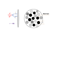
Figure 1: A transverse view of a high–energy hadron, as ‘seen’ in deep inelastic scattering at very high energy. The dipole projectile probes a target area of the order of its own transverse area, at various impact parameters.

This new picture has rich and interesting consequences: it leads to a total breakdown of the ‘twist expansion’ up to very high values for $Q^{2}$ and it predicts a new scaling law for $\langle T(Q^{2})\rangle$ at high energies [1, 2, 9] — known as diffusive scaling [7] —, which should replace the geometric scaling expected [10, 11, 12] from mean field approximations like the Balitsky–Kovchegov equation [13, 14] or the more general (functional) JIMWLK equation [15, 16, 17].

The strong fluctuations in the gluon distribution at high energy find their origin in gluon–number fluctuations in the early stages of the evolution, i.e., BFKL–like [18, 19] splitting processes, which induce correlations between the gluons having a common ancestor, and thus between the ‘spots’ generated via the subsequent evolution of these gluons. So far, the effects of these correlations have been studied only at fixed impact parameter, via a coarse–graining of the Pomeron loop equations in impact–parameter space [1, 2]. This approximation is perhaps sufficient for a study of the scattering of a small projectile which is quasi–localized in $\bm{b}$ (e.g., the case of the dipole scattering, as relevant for $\gamma^{*}p$ deep inelastic scattering [7], and also for $pp$ or $pA$ collisions under specific circumstances [8]), but on the other hand it prevents one from studying the correlations in $\bm{b}$, which could be experimentally accessed via multiple–particle production in hadron–hadron collisions (say, at LHC). Moreover, as we shall later argue, this approximation has some shortcomings even for the description of the short–range correlations, for which it was a priori intended: by ignoring any information about the size of the fluctuations in impact–parameter space, it artificially suppresses the fluctuations with very small sizes, i.e., the tiny spots where the local saturation momentum is much larger than the average one. Or, as alluded to before, a proper description of such tiny spots is essential in order to study the scattering of small projectiles with resolution $Q^{2}\gg Q_{s}^{2}$.

In this paper, we shall make a first attempt to go beyond the coarse–graining approximation introduced in Refs. [1, 2]. Namely, we shall propose an effective field theory describing the distribution of the saturation momentum in impact–parameter space at a fixed (high) energy and for a large number of colors $N_{c}$. (The large–$N_{c}$ approximation is needed in order to be able to neglect long–range color exchanges between saturated spots; see Sect. 2 for details.) Note that the saturation momentum $Q_{s}(\bm{b})$ is also the typical transverse momentum of the gluon configuration located around $\bm{b}$. Hence, the effective theory that we shall propose encodes information about the gluon distributions in both momentum space and impact–parameter space.

Let us start by emphasizing that the very existence of an effective field theory for $Q_{s}(\bm{b})$ is not at all obvious. For instance, it is not a priori clear whether one can effectively replace (even if only approximately) the information about the gluon distribution or the dipole scattering amplitudes by a theory for the distribution of the saturation momentum alone. Furthermore, even assuming that such a theory exists, it is not at all clear whether it can be made local. The Pomeron loop equations are non–local in the transverse momenta and coordinates, and this may translate into non-localities in $\bm{b}$ in the effective theory that we are looking for. Moreover, the correlations induced by the evolution are generally non–local in rapidity, since associated with gluon splittings in the intermediate steps of the evolution. Still, as we shall argue in Sect. 2, the short–range correlations, at least, are quasi–local in rapidity, since predominantly produced via gluon splittings in the late stages of the evolution, close to the final rapidity $Y$. By ‘short–range’ we mean distances of the order of, or smaller than, the average saturation length $1/Q_{0}(Y)$ at rapidity $Y$ (with the notation $Q_{0}^{2}\equiv\langle Q_{s}^{2}\rangle$). Hence, we expect a local field theory to be meaningful, at least, for the dynamics over such short distances.

To proceed, we shall simply assume that a local field theory for $Q_{s}(\bm{b})$ exists and then we shall constrain its structure from general physical considerations. More precisely, we shall construct this theory as the natural generalization of the $\bm{b}$–independent distribution proposed in Refs. [1, 2] which is consistent the uncertainty principle and the conformal symmetry of the high–energy evolution equations. Together, these constrains almost uniquely fix the structure of the effective theory, as we explain now:

As already mentioned, the saturation momentum $Q_{s}(\bm{b})$ is also the typical transverse momentum of the gluon configuration centered at $\bm{b}$. By virtue of the uncertainty principle, the area occupied by that configuration cannot be smaller than $1/Q_{s}^{2}(\bm{b})$. This area cannot be much larger either, since a gluon configuration which has reached saturation on some scale $Q_{s}(\bm{b})$ can hardly emit gluons with soft momenta $k_{\perp}\ll Q_{s}(\bm{b})$ [22, 23, 24, 25]. That is, its subsequent evolution predominantly proceeds via the emission of harder gluons with $k_{\perp}\gg Q_{s}(\bm{b})$, which cannot increase the size of the configuration (except very slowly, via peripheral emissions). In turn, such hard gluons become spots which evolve towards saturation on their own sizes and at the same time act as sources for even smaller spots, which spread over the surface of the original configuration and where the local saturation momenta are much harder. We see that the high–energy evolution is strongly biased towards smaller sizes, thus leading — in a three–dimensional picture where the impact–parameter space occupies the $(x,y)$–plane and the saturation momentum $Q_{s}(\bm{b})$ is represented along the $z$–axis — to a ‘landscape’ picture, with spikes of various heights, randomly distributed and surrounded by valleys.

Furthermore, the equations describing the evolution in QCD at high energy and in the leading logarithmic approximation have the important property of conformal symmetry, that is, they are invariant under conformal (Möbius) transformations in the transverse plane. This has since long been appreciated in the context of the linear, BFKL, evolution [18], with important consequences [26, 27, 28] (in particular, for the calculability of the theory; see Ref. [29] for a review and more references), but this remains true for the non–linear BK [13, 14], JIMWLK [15, 16, 17], or Pomeron loop [2, 3, 4], equations, since all these equations involve the BFKL splitting kernel (for gluons or dipoles) together with gluon–number changing vertices, which indeed respect conformal symmetry. One may think that this symmetry is inconsistent with the emergence of a special scale — the (average) saturation momentum — in the solutions to these equations, but this is actually not true: the saturation scale is not spontaneously generated by the evolution, rather it comes out as the evolution of the scale introduced by the initial conditions at low energy [21, 23, 10, 11]. On the other hand, the gluon correlations are generated by the conformally–invariant evolution, so we expect this symmetry to constrain the effective theory describing these correlations.

The effective theory that we shall arrive at by exploiting such considerations is a two–dimensional, interacting, scalar field theory, in which the field $\phi$ is proportional to the logarithm of the local saturation momentum, and which involves two ‘free’ parameters: the expectation value $Q_{0}^{2}\equiv\langle Q_{s}^{2}\rangle$ of the saturation momentum and a dimensionless coupling constant $\sigma$, which characterizes the degree of disorder introduced by gluon–number fluctuations in the course of the evolution. Both parameters are expected to rise with the energy, in a way which is in principle determined by the underlying QCD evolution equations, but which needs not be specified for our present purposes. It suffices to say that the weak coupling regime $\sigma\ll 1$ in the effective theory corresponds to low, or intermediate, energies, where the dynamics is quasi–deterministic, whereas the strong coupling regime $\sigma\gg 1$ corresponds to the more interesting situation at high energy, where the stochastic aspects are fully developed and essential.

The effective theory involves three basic ingredients: (i) the standard kinetic term, which couples fluctuations at neighboring points, (ii) a potential term, which ensures that the typical gradients at $\bm{b}$ are of order $Q_{s}^{2}(\bm{b})$, in fulfillment of the uncertainty principle, and (iii) a source term, which enforces the value $Q_{0}^{2}\equiv\langle Q_{s}^{2}(\bm{b})\rangle$ of the average saturation momentum. Since proportional to $Q_{s}^{2}\propto{\rm e}^{\sigma\phi}$, the potential is exponential in $\phi$, which is precisely as it should for consistency with conformal symmetry: together, the kinetic plus the potential terms are recognized as the Liouville action, which is conformally–invariant, and thus integrable. The quantum Liouville field theory (LFT) has been extensively studied over the last decades — especially, in connection with studies of quantum gravity in two dimensions — and many exact results are known by now about its properties [30, 31, 32, 33, 34, 35]. However, precisely by virtue of its symmetry, LFT involves no mass scale (it gives rise to power–law correlations on all distance scales), and thus cannot accommodate a non–zero value for the average saturation momentum. This is taken care off by the source term, linear in $\phi$, at the expense of explicitly breaking the conformal symmetry. This breaking has dramatic consequences on the properties of the theory and it also complicates its analysis very much (since it is not possible to directly exploit the large amount of information known about LFT).

Yet, some general properties of the effective theory can be inferred by semi–classical and perturbative techniques, or simply by inspection of the action. The presence of the source term endows this theory with a stable ground state (in contrast to LFT), which appears as a saddle point of the action and allows for a perturbative treatment of the weak coupling ($\sigma\ll 1$) regime. The perturbative calculations, that we shall push up to two–loop order, reveal a very interesting property, which is furthermore confirmed, at non–perturbative level, by inspection of the corresponding Dyson equations: the correlations of the saturation momentum (an exponential operator in this theory) are ultraviolet finite, and not just renormalizable, as generally expected for a two–dimensional field theory. This means that the operator $Q_{s}^{2}$ has no anomalous dimension, which in turn implies that its short–range correlations, over distances $R\mathrel{\hbox to0.0pt{\raise 2.20013pt\hbox{$<$}\hss}{\lower 2.20013pt\hbox{$\sim$}}}1/Q_{0}$, have a power–like decay, with exactly the same powers as in pure Liouville theory — since these powers are fixed by the natural dimension of the operator. On the other hand, the theory predicts that these correlations decay exponentially on larger distances $R\gg 1/Q_{0}$, with the (average) saturation momentum $Q_{0}$ playing the role of a screening mass. The emergence of an exponential fall–off in the context of perturbative QCD may look surprising, but it is presumably an artifact of our insistence on a field theory which is local in rapidity: the physical correlations on large distances $R\gg 1/Q_{0}$ are typically generated via gluon splittings in the early stages of the evolution (the earlier, the larger $R$ is; see Sect. 2)), which are not encoded in our present theory.

The paper is organized as follows: Sect. 2 presents a brief and critical discussion of the $\bm{b}$–independent distribution proposed in Refs. [1, 2], with the purpose of clarifying its limitations and, more generally, the limitations of any effective theory which is local in rapidity. In Sect. 3 we construct the low–energy/weak coupling ($\sigma\ll 1$) version of the effective field theory, as the straightforward extension of the $\bm{b}$–independent distribution alluded to above. Sect. 4 is our main section: after a quick introduction to the Liouville field theory and its conformal symmetry, we explain the relevance of this theory for the QCD problem at hand, then present the complete action for our effective theory (including the symmetry–breaking source term) and discuss some of its properties. Sect. 5 is slightly more technical, since devoted to perturbative calculations to two–loop order, with the purpose of demonstrating the ultraviolet–finiteness of the correlation functions when computed in the effective theory. Finally, Sect. 6 summarizes our results and conclusions. In the Appendix, we show how to couple the effective theory to the CGC formalism (within the simple context of McLerran–Venugopalan model [36]), which is useful in view of computing observables.

2 The coarse–graining approximation and its limitations

Our starting point is the Gaussian probability distribution for the saturation momentum introduced in Refs. [1, 2] (see also Refs. [37, 38, 39]), which can be viewed as a coarse–grained version of the effective theory that we intend to construct, in which the impact–parameter dependence has been averaged out. The applicability of such a coarse–graining will be shortly discussed.

The random variable in this distribution is the logarithm $\rho_{s}\equiv\ln(Q_{s}^{2}/\Lambda^{2})$ of the saturation momentum (with $\Lambda$ some arbitrary scale of reference), which is the scale which separates, in an event–by–event description, between a high–density, or ‘Color Glass Condensate’ [40], phase at low transverse momenta ($k_{\perp}<Q_{s}$ or $\rho\equiv\ln(k_{\perp}^{2}/\Lambda^{2})<\rho_{s}$), where the gluon occupation factor saturates at a large value of $\mathcal{O}(1/\alpha_{s})$, and a low density phase at high momenta ($\rho>\rho_{s}$), where the gluon occupancy is still low but it rises rapidly with the energy (as a power of $s$), via BFKL gluon splitting. It is customary to work with the ‘rapidity’ variable $Y\equiv\ln s$, which plays the role of an ‘evolution time’ for the high–energy evolution. When increasing $Y$, modes with higher and higher values of $k_{\perp}$ enter at saturation, so the borderline $\rho_{s}$ propagates towards higher transverse momenta. However, due to gluon–number fluctuations in the splitting process — which can be associated with the fact that the particle number is discrete [1] —, this progression of $\rho_{s}$ is not uniform but stochastic, like a one–dimensional Brownian motion.

Based on the analogy with the reaction–diffusion problem [37, 41, 38, 39], it has been argued in Refs. [1, 2] that $\rho_{s}$ should be a Gaussian random variable with probability distribution

$$P_{Y}(\rho_{s})=\frac{1}{\sqrt{2\pi}\sigma}\,\exp\left[-\frac{\left(\rho_{s}-\langle\rho_{s}\rangle\right)^{2}}{2\sigma^{2}}\right]\,,$$ (2.1)

where both the central value $\langle\rho_{s}\rangle$ and the dispersion $\sigma^{2}=\left\langle\rho_{s}^{2}\right\rangle-\langle\rho_{s}\rangle^{2}$ are expected to rise linearly with $Y$ (for $Y$ large enough): $\langle\rho_{s}\rangle=\lambda\bar{\alpha}_{s}Y$ and $\sigma^{2}\simeq D\bar{\alpha}_{s}Y$, with $\bar{\alpha}_{s}\!=\!\alpha_{s}N_{c}/\pi$. The coefficients $\lambda$ and $D$ are known [37, 38] only in the formal limit $\alpha_{s}\to 0$, and the corresponding expressions cannot be extrapolated to realistic values of $\alpha_{s}$ since they depend upon $\ln(1/\alpha_{s}^{2})$. For what follows, their actual values are unimportant, and so are the precise $Y$–dependencies of $\langle\rho_{s}\rangle$ and $\sigma$; all that matters is that these quantities rise quite fast with $Y$. So long as $\sigma\ll 1$ — the case for relatively low energies — the theory remains quasi–deterministic. But the most interesting regime for us here is the high–energy regime at $\sigma\geq 1$, where the fluctuations are fully developed and have a strong influence on the theory.

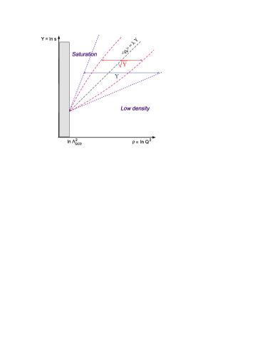
Figure 2: A picture of the diffusive saturation boundary in the presence of fluctuations; shown are the average saturation line $\langle\rho_{s}\rangle=\lambda\bar{\alpha}_{s}Y$, the diffusive radius $\sigma\propto\sqrt{Y}$ for the Gaussian distribution (2.1), and the diffusive scaling window with a width $\sigma^{2}\propto Y$.

Since the saturation momentum is fluctuating, a physical discussion will naturally involve a range of values for $Q_{s}$, rather than just a single value (see Fig. 2). The range which is a priori privileged by the Gaussian probability (2.1) is the ‘diffusive disk’ at $|\rho_{s}-\langle\rho_{s}\rangle|\leq\sigma$, where the probability is reasonably large: $P(\rho_{s})\mathrel{\hbox to0.0pt{\raise 2.20013pt\hbox{$>$}\hss}{\lower 2.20013pt\hbox{$\sim$}}}1/\sigma$. But the relevant range also depends upon the physical quantity of interest, which can favor some values of $Q_{s}$ over the others. The simplest example in that sense refers to the very definition of the ‘average saturation momentum’, which is not unique (because the relation between $Q_{s}$ and $\rho_{s}$ is non–linear: $Q_{s}^{2}=\Lambda^{2}{\rm e}^{\rho_{s}}$) and thus needs to be properly specified — different definitions can be relevant for different problems. The form of the Gaussian distribution (2.1) makes it natural to define

$$\bar{Q}_{s}^{2}\,\equiv\,\Lambda^{2}\,{\rm e}^{\langle\rho_{s}\rangle}\,.$$ (2.2)

But the expectation value of the ‘operator’ ${\rm e}^{\rho_{s}}$ can be also computed, with the following result:

$$\langle Q_{s}^{2}\rangle\,\equiv\,\Lambda^{2}\,\langle{\rm e}^{\rho_{s}}\rangle\,=\,\Lambda^{2}\,{\rm e}^{\langle\rho_{s}\rangle}\,{\rm e}^{\frac{1}{2}\sigma^{2}}\,=\,\bar{Q}_{s}^{2}\,\,{\rm e}^{\frac{1}{2}\sigma^{2}}\,.$$ (2.3)

This is always harder than the scale in Eq. (2.2), and for sufficiently high energies, where $\sigma\gg 1$, it is even much harder. This considerable difference between the two definitions can be easily traced back: in computing $\langle Q_{s}^{2}\rangle$, the exponential operator ${\rm e}^{\rho_{s}}$ biases the integration towards very large values of $\rho_{s}$, of order $\rho_{s}\sim\langle\rho_{s}\rangle+\sigma^{2}$, as opposed to the typical value $\rho_{s}\sim\langle\rho_{s}\rangle$ contributing to $\bar{Q}_{s}^{2}$. Note that the large deviation $\rho_{s}-\langle\rho_{s}\rangle\sim\sigma^{2}$ corresponds to fluctuations which are very rare: $P(\rho_{s})\sim\exp(-\sigma^{2}/2)\ll 1$, and which occupy a very small area $\sim 1/\langle Q_{s}^{2}\rangle$ in impact–parameter space (by the uncertainty principle). Yet, such rare and tiny fluctuations are physically important, as they define the upper bound of the diffusive scaling window [2, 7, 8]:

$$-\frac{\sigma^{2}}{2}\,\ll\,\rho-\langle\rho_{s}\rangle\,\ll\,\frac{\sigma^{2}}{2}\,,$$ (2.4)

(see also Fig. 2) where $\rho\equiv\ln(Q^{2}/\Lambda^{2})$, with $Q^{2}$ the transverse resolution of a small projectile, like a ‘color dipole’ (a $q\bar{q}$–pair fluctuation of the virtual photon in deep inelastic electron–hadron scattering), which scatters off the hadron. The interval in Eq. (2.4) represents the kinematical window at high energy ($\sigma\gg 1$) within which the (average) dipole scattering amplitude $\langle T(\rho,Y)\rangle$ ‘scales’ as a function of the dimensionless variable $Z\equiv(\rho-\langle\rho_{s}\rangle)/\sigma$ rather than separately depending upon $\rho$ and $Y$ : $\langle T(\rho,Y)\rangle\approx\langle T(Z)\rangle$ (see Refs. [2, 7, 8] for details). The diffusive scaling window in Eq. (2.4) can be alternatively described as

$$\bar{Q}_{s}^{2}\,{\rm e}^{-\frac{1}{2}\sigma^{2}}\,\ll\,\,Q^{2}\,\ll\,\,\bar{Q}_{s}^{2}\,{\rm e}^{\frac{1}{2}\sigma^{2}}\equiv\,\langle Q_{s}^{2}\rangle\,,$$ (2.5)

which explicitly shows that both definitions for the ‘average saturation momentum’ introduced in Eqs. (2.2) and, respectively, (2.3) play a role in characterizing the physical effects of the fluctuations in $Q_{s}$.

At this point one should remember that the previous discussion was based on the local approximation (2.1) for the distribution of $Q_{s}$, so it is important to understand what are the assumptions beyond this approximation. In Refs. [1, 2] (see, especially, the discussion in Sect. 6 of Ref. [2]), the distribution (2.1) has been obtained via a coarse–graining in impact–parameter space: the $\bm{b}$–dependence of the dipole scattering amplitudes, as encoded in the Pomeron loop equations [4, 3], has been averaged out over a region in the impact–parameter space which in Refs. [1, 2] has been loosely characterized as the ‘dipole size’, but which should be more properly interpreted as an intrinsic scale in the hadron, so like $1/\bar{Q}_{s}$. In this averaging, one has potentially neglected two types of correlations: (i) short–range correlations between the fluctuations (‘spots’) with small sizes $R\ll 1/\bar{Q}_{s}$ (i.e., with large saturation momenta $Q_{s}\gg\bar{Q}_{s}$) which lie inside the coarse–graining cell — such smaller spots were treated as being uniformly distributed over the cell area $1/\bar{Q}_{s}^{2}$, and (ii) the long–range ($R\gg 1/\bar{Q}_{s}$) correlations between different cells. Besides, one has assumed homogeneity in $\bm{b}$ — the average saturation momentum $\bar{Q}_{s}^{2}$ and the dispersion $\sigma^{2}$ were taken to be independent of $\bm{b}$ —, which is not really an approximation, but merely a choice for the initial conditions at low energy (the homogeneity being preserved by the evolution according to the Pomeron loop equations). Under these assumptions, the $\bm{b}$–dependence has disappeared from the evolution equations, which were then shown [2] to be equivalent to a stochastic equation of the sFKPP type — the Langevin equation for the reaction–diffusion process [41]. The Gaussian probability distribution in Eq. (2.1) then follows from known properties of the sFKPP equation, as recently clarified in the respective literature [37, 38, 39].

Thus, the fact that here is no explicit $\bm{b}$–dependence in Eq. (2.1) must be understood as follows: this formula is meant to apply to points $\bm{b}$ within a given coarse–graining cell, with an area $\sim 1/\bar{Q}_{s}^{2}\,$; at all such points, the event–by–even local saturation scale is assumed to be the same, and equal to $\rho_{s}$ (in logarithmic units); that is, all the points within a cell fluctuate coherently with each other, so like a rigid body. On the other, nothing is said about the correlations between different cells: Eq. (2.1) apply only to local fluctuations within a given cell, as averaged over the size of that cell.

How does this approximate picture compare with the physical reality ? There are a priori two mechanisms for building spot–spot correlations: (a) Long–range interactions between saturated spots: A gluon configuration with saturation momentum $Q_{s}$ has a low but non–zero probability to emit low–momentum gluons with $k_{\perp}\ll Q_{s}$, thus creating long–range color fields over distances $R\gg 1/Q_{s}$. These are dipolar fields, and not Coulomb ones, because the total color charge gets screened at saturation [24, 42, 25]. These fields mediate dipole–dipole interactions between saturated spots which are far away from each other. However, these interactions are suppressed by a factor $1/N_{c}^{2}$, as they imply color exchanges, and thus can be safely neglected in the large–$N_{c}$ approximation underlying the present discussion. (b) Gluon–number fluctuations in the high–energy evolution: As mentioned in the Introduction, different spots can be correlated with each other because they have a common ancestor at some earlier rapidity. Such correlations survive at large $N_{c}$, since associated with fluctuations in a colorless quantity: the number of gluons in the light cone gauge. Eq. (2.1) is meant to capture these fluctuations in the coarse–graining approximation, and our purpose here is to relax this approximation by restoring the $\bm{b}$–dependence of the induced correlations.

However, as also mentioned in the Introduction, the relevant correlations are generally non–local in rapidity, since induced through branching processes which can occur at all the intermediate rapidities. As we shall explain now, the short–range correlations generated in this way can nevertheless be encoded in a local (in $Y$) field theory, of the type we would like to construct. To that aim, we shall consider two spots which are separated by a distance $R$ at the final rapidity $Y$. These spots are correlated with each other provided they had a common ancestor at some earlier rapidity $0<y<Y$. It turns out that $y$ is correlated with $R$. Indeed, the typical spots at rapidity $y$ have a saturation momentum $\bar{Q}_{s}(y)$ and a size $\sim 1/\bar{Q}_{s}(y)$. If that size is much smaller than $R$, then such a typical spot has only little probability to emit a gluon at a distance $R$ away from its center and thus initiate the evolutions leading to the two final spots that we measure at $Y$. (This probability decreases as a large power of $(R\bar{Q}_{s}(y))^{-1}$ because of the screening of the color charge at saturation.) If, on the other hand, $1/\bar{Q}_{s}(y)\gg R$, then there is a geometrical penalty factor $\sim(R\bar{Q}_{s}(y))^{2}$ for the gluon to be emitted inside the (relatively small) domain with area $R^{2}$. Hence, the most important intermediate rapidity $y$ for creating correlations over a distance $R$ is the one for which $\bar{Q}_{s}(y)\sim 1/R$. Therefore, the larger is $R$, the more we have to go backwards in the evolution, and the more non–local are the respective correlations in $Y$. Vice–versa, the short–range correlations with $R\mathrel{\hbox to0.0pt{\raise 2.20013pt\hbox{$<$}\hss}{\lower 2.20013pt\hbox{$\sim$}}}1/\bar{Q}_{s}(Y)$ are typically produced in the late stages of the evolution, at $y\sim Y$, and hence are quasi–local in rapidity. It should be therefore possible to encode such short–range correlations in a local, effective, field theory.

As we shall later see, these considerations are indeed consistent with the effective field theory that we shall arrive at, except for the fact that the actual scale for correlations which will emerge from that theory is not the scale $\bar{Q}_{s}^{2}$ that we have focused on in the above discussion, but rather the harder scale $\langle Q_{s}^{2}\rangle$, cf. Eq. (2.3).

3 The effective field theory: weak coupling

With this section, we start our program aiming at extending the coarse–grained distribution in Eq. (2.1) to an effective field theory which describes the distribution of the saturation momentum in impact–parameter space. For more clarity, we shall first develop our arguments for the low energy/weak coupling regime $\sigma\ll 1$, where we shall argue that the corresponding extension is a free field theory for a massive scalar field in two (Euclidean) dimensions. Then, in Sect. 4, we shall present the generalization of this theory to arbitrary values of the coupling $\sigma$.

For more clarity, we shall assume ‘mean-field–like’ initial conditions at low energy ($Y=0$): the initial gluon density is large and homogeneous, and the saturation momentum $Q_{s}(Y=0)$ takes the same value $\Lambda$ (with $\Lambda^{2}\gg\Lambda^{2}_{\rm QCD}$) at all the points. By boosting this system to high energy, the gluon distribution evolves via (generally, non–linear) gluon splitting, and inhomogeneities (‘spots’) appear in the event–by–event description, due to gluon–number fluctuations.

In the early stages of this evolution — namely, so long as $\sigma\ll 1$ —, the fluctuations have no time to significantly develop, so all the spots have more or less the same size, $\sim 1/\bar{Q}_{s}$, and the same value for the saturation momentum, $\sim\bar{Q}_{s}$; furthermore, they are only weakly correlated with each other. It is then straightforward to extend the coarse–grained approximation (2.1) to a distribution which covers the whole transverse profile of the hadron: this is simply the product of independent Gaussian distributions like that in Eq. (2.1), one for each spot :

$$P_{Y}[\rho_{s}]=\prod_{j}\frac{1}{\sqrt{2\pi}\sigma}\,\exp\left[-\frac{\left(\rho_{s}(j)-\langle\rho_{s}\rangle\right)^{2}}{2\sigma^{2}}\right]\quad\mbox{for}\quad\sigma\ll 1\,,$$ (3.1)

where the discrete variable $j$ labels the spots, and each spot has roughly an area $1/\bar{Q}_{s}^{2}$. Introducing the fluctuation field $\eta(j)\equiv\rho_{s}(j)-\langle\rho_{s}\rangle$, Eq. (3.1) implies: $\langle\eta(j)\eta(l)\rangle=\sigma^{2}\delta_{lj}$. So far, the quantities $\rho_{s}(j)$ or $\eta(j)$ refer globally to a spot. In order to promote them to field variables $\rho_{s}(\bm{x})$ or $\eta(\bm{x})$, with $\bm{x}$ denoting the impact parameter, but keep the same correlations as above, one needs to introduce a kinetic term to smear out correlations over the spot size $\sim 1/\bar{Q}_{s}$. The simplest kinetic term, and also the only one to be renormalizable in two dimensions, is the standard, quadratic, kinetic term, that we shall adopt in what follows. We are thus led to the following field–theoretical extension of Eq. (3.1)

$$P_{Y}[\eta]\,=\,\exp\left\{-S_{0}[\eta]\right\},\quad\mbox{with}\quad S_{0}[\eta]\equiv\,\frac{1}{2\sigma^{2}}\int{\rm d}^{2}\bm{x}\left\{(\nabla^{i}\eta)^{2}+\bar{Q}_{s}^{2}\eta^{2}\right\}\,,$$ (3.2)

which provides the weight function for the functional integral over $\eta(\bm{x})$ which defines expectation values in the framework of this effective field theory. The measure in the functional integral is assumed to carry the proper normalization: $\int D[\eta]\,\exp\left\{-S_{0}[\eta]\right\}=1$.

Eq. (3.2) implies $\langle\eta(\bm{x})\eta(\bm{y})\rangle=\sigma^{2}\,D(\bm{x}-\bm{y})$, with $D$ the propagator of a free, massive, scalar field in a two–dimensional Euclidean space:

$$D(\bm{x-y})=\int\frac{{\rm d}^{2}\bm{k}}{(2\pi)^{2}}\,\frac{{\rm e}^{i\bm{k}\cdot\bm{(x-y)}}}{k^{2}+\bar{Q}_{s}^{2}}\,=\,\frac{1}{2\pi}\,{\rm K}_{0}(r\bar{Q}_{s})$$ (3.3)

where $r=|\bm{x-y}|$ and ${\rm K}_{0}$ is the respective Bessel function, with the following limiting behaviours at short and, respective, large distances:

$${\rm K}_{0}(z)\approx\,\begin{cases}\displaystyle{\ln\frac{1}{z}\,,}&\text{ for\, $z\ll 1$}\\[14.22636pt] \displaystyle{\sqrt{\frac{\pi}{2z}}{\rm e}^{-z}\,,}&\text{ for\, $z\gg 1$}.\end{cases}$$ (3.4)

We see that the correlations generated by the field theory in Eq. (3.2) have indeed the sought for structure: they are quasi–uniform on relatively short distances, $r\mathrel{\hbox to0.0pt{\raise 2.20013pt\hbox{$<$}\hss}{\lower 2.20013pt\hbox{$\sim$}}}1/\bar{Q}_{s}$, (i.e., among points located within a same spot), but they decay very fast (exponentially) over distances much larger than the typical size of a spot.

The emergence of exponentially decaying correlations at large distances should be taken with a grain of salt (cf. the discussion in the Introduction): It corresponds to the fact that the correlations over larger distances $r\gg 1/\bar{Q}_{s}$ are predominantly produced via splittings occuring in the early stages of the evolutions, i.e., at rapidities $y<Y$, whose effects are not included in the present formalism, local in $Y$. As for the late splittings (those taking place at $y\sim Y$), they produce correlations which fall off according to power laws at large separations $r\gg 1/\bar{Q}_{s}$, because the emissions of soft gluons with $k_{\perp}\ll\bar{Q}_{s}(Y)$ is strongly suppressed by saturation. The fact that, in our formalism, this fall–off appears to be exponential, rather than power–like, is because we have not provided a faithful description of the gluon spectrum, including its softening at momenta below $Q_{s}$, but rather we have replaced this whole spectrum by a unique scale — the saturation momentum —, which represents the average transverse momentum of the saturated gluons. To summarize this argument, the theory with action (3.2) provides the correct, logarithmic, behaviour at short distances, and it mimics the rapid fall–off at larger distances by an exponential tail, rather than the correct, power–law, one. This will be a generic feature of the effective theory, including at strong coupling.

We now return to the functional distribution in Eq. (3.2) and consider its predictions for the correlation functions of the operator saturation momentum, $Q_{s}^{2}(\bm{x})\equiv\Lambda^{2}{\rm e}^{\rho_{s}}=\bar{Q}_{s}^{2}{\rm e}^{\eta}$. One finds

$$\langle Q_{s}^{2}(\bm{x})\rangle \,=\, \bar{Q}_{s}^{2}\,\,{\rm e}^{\frac{1}{2}\sigma^{2}D(0)}\,,$$

$$\langle Q_{s}^{2}(\bm{x})Q_{s}^{2}(\bm{y})\rangle \,=\, \bar{Q}_{s}^{4}\,\,{\rm e}^{\sigma^{2}[D(0)+D(\bm{x}-\bm{y})]}\,,$$ (3.5)

etc. Strictly speaking, these expressions should be trusted only up to terms of $\mathcal{O}(\sigma^{2})$, since we are working under the assumption that $\sigma\ll 1$; notwithstanding, we here display the full exponentials, for comparison with subsequent results at strong coupling.

The above formulæ involve the equal–point limit $D(0)$ of the propagator, which is divergent: $D(0)=({1}/{2\pi})\ln({1}/{a\bar{Q}_{s}})$, with $a$ a short–distance cutoff (‘lattice spacing’) introduced to regularize the divergence. We see that, even within this free field theory, the exponential (or ‘vertex’) operator $V(\bm{x})\equiv{\exp}\{\eta(\bm{x})\}$ develops ultraviolet divergences, which arise from contractions internal to this operator. As is well known [43], and also manifest on Eq. (3), such divergences can be eliminated via multiplicative renormalization of the vertex operator (which here is tantamount to normal–ordering the polynomial operators which appear in its expansion). Namely, we shall define the renormalized vertex operator as

$$V_{R}(\bm{x})\equiv V(\bm{x})\,{\exp}\left\{\frac{\sigma^{2}}{4\pi}\ln\left(a{\rm e}^{2\pi}\bar{Q}_{s}\right)\right\}\,=\,{\exp}\left\{\frac{\sigma^{2}}{2}[1-D(0)]\right\}\,{\rm e}^{\eta(\bm{x})}\,,$$ (3.6)

where the particular subtraction point $1/a={\rm e}^{2\pi}\bar{Q}_{s}$ has been chosen for reasons to shortly become clear. One then obtains the following, finite, vertex correlation functions:

$$\langle V_{R}(\bm{x})\rangle\,=\,{\rm e}^{\frac{1}{2}\sigma^{2}},\ \dots\ ,\ \langle V_{R}(\bm{x}_{1})\cdots V_{R}(\bm{x}_{n})\rangle\,=\,{\exp}\Big{\{}\frac{n}{2}\sigma^{2}+\sigma^{2}\sum_{i<j}D(\bm{x}_{i}-\bm{x}_{j})\Big{\}}\,,$$ (3.7)

which in turn imply, for the renormalized operator $Q_{s}^{2}(\bm{x})\equiv\bar{Q}_{s}^{2}\,V_{R}(\bm{x})$,

$$\langle Q_{s}^{2}(\bm{x})\rangle \,=\, \bar{Q}_{s}^{2}\,\,{\rm e}^{\frac{1}{2}\sigma^{2}}\,,$$

$$\langle Q_{s}^{2}(\bm{x})Q_{s}^{2}(\bm{y})\rangle \,=\, \bar{Q}_{s}^{4}\,\,{\rm e}^{\sigma^{2}+\sigma^{2}D(\bm{x}-\bm{y})}\,=\,\langle Q_{s}^{2}\rangle^{2}\,{\rm exp}\{\sigma^{2}D(\bm{x}-\bm{y})\}\,.$$ (3.8)

One can now appreciate the particular choice for the subtraction point in Eq. (3.6): this is such that the expectation value $\langle Q_{s}^{2}\rangle$ computed in the present field theory precisely matches the corresponding prediction of the coarse–grained approximation, cf. Eq. (2.3).

Interestingly, Eq. (3) reveals the emergence of power–like correlations over (relatively) short distances, that is, in between the points lying inside a same spot:

$$\langle Q_{s}^{2}(\bm{x})Q_{s}^{2}(\bm{y})\rangle\,\approx\,\frac{\langle Q_{s}^{2}\rangle^{2}}{\big{[}|\bm{x-y}|\bar{Q}_{s}\big{]}^{{\sigma^{2}}/{2\pi}}}\qquad\mbox{for}\qquad|\bm{x-y}|\ll 1/\bar{Q}_{s}\,.$$ (3.9)

This exhibits a singularity in the equal–point limit, which is however physical, in the sense that one cannot localize fluctuations in a quantum field theory down to a point without generating singularities. On the other hand, at large distances, the connected piece of the 2–point function in Eq. (3) dies away exponentially:

$$\langle Q_{s}^{2}(\bm{x})Q_{s}^{2}(\bm{y})\rangle-\langle Q_{s}^{2}\rangle^{2}\,\propto\,\,\sigma^{2}\langle Q_{s}^{2}\rangle^{2}\exp(-|\bm{x-y}|\bar{Q}_{s})\quad\ \mbox{for}\quad\ |\bm{x-y}|\gg 1/\bar{Q}_{s}\,.$$ (3.10)

Once again, this exponential decay should be taken with a grain of salt: the effective theory is not supposed to apply to such large separations.

4 The effective field theory: general case

Although this has not been explicitly spelled out in the previous discussion, the free field theory of Eq. (3.2) is indeed consistent with the uncertainty principle in the regime where this theory is meant to apply (i.e., for $\sigma\ll 1$): indeed, the kinetic term there smears out inhomogeneities over the very short distances $r\ll 1/\bar{Q}_{s}$, in agreement with the fact that the size of a spot cannot be smaller than the inverse of the typical momentum of the gluons composing that spot, namely $k_{\perp}\sim\bar{Q}_{s}$. However, for sufficiently high energy, such that $\sigma\mathrel{\hbox to0.0pt{\raise 2.20013pt\hbox{$>$}\hss}{\lower 2.20013pt\hbox{$\sim$}}}1$, the fluctuations become important and then the actual saturation momentum $Q_{s}^{2}(\bm{x})$ at a given point and in a given event can be very different from any of its expectation values ($\bar{Q}_{s}^{2}$ or $\langle Q_{s}^{2}\rangle$) previously introduced. In such a case, the uncertainty principle requires that the minimal size of a spot located at $\bm{x}$ be fixed by the actual value $Q_{s}^{2}(\bm{x})$ of the saturation momentum, and not by its expectation value. This means that, in the general action for $\eta$, the kinetic term should compete with the actual (event–by–event) saturation momentum, and not with its ‘expectation value’ (whatever the meaning of the latter is).

Accordingly, the effective ‘mass term’ in the action should be the field–dependent scale $Q_{s}^{2}(\bm{x})\equiv\bar{Q}_{s}^{2}\,{\exp}\{\eta(\bm{x})\}$. This argument suggests the following generalization of Eq. (3.2):

$$S_{1}[\eta]\equiv\,\frac{1}{2\sigma^{2}}\int{\rm d}^{2}\bm{x}\left\{(\nabla^{i}\eta)^{2}+\bar{Q}_{s}^{2}\eta^{2}{{\rm e}}^{\eta}\right\}\,,$$ (4.1)

which involves an exponential potential. Clearly, this is now an interacting field theory in which the parameter $\sigma$ — which, we recall, is a measure of the dispersion introduced by fluctuations — plays the role of a coupling constant, as it can be recognized after rescaling $\eta\equiv\sigma\phi$ :

$$S_{1}[\phi]=\int{\rm d}^{2}\bm{x}\left\{\frac{1}{2}(\nabla^{i}\phi)^{2}+\frac{1}{2}\,\bar{Q}_{s}^{2}\phi^{2}{{\rm e}}^{\sigma\phi}\right\}\,.$$ (4.2)

Strong interactions for the field $\phi$ correspond to strong correlations between spots with different sizes and at different locations, as physically expected at sufficiently high energy. However, it should be clear that the precise form of the potential for $\phi$, beyond the exponential factor, cannot be uniquely fixed by the uncertainty principle alone: a factor of $\phi$ counts like $\ln Q_{s}$ and hence it cannot modify the power–counting argument that $\nabla^{2}\sim Q_{s}^{2}$. Thus, the uncertainty principle alone would allow for any potential where ${{\rm e}}^{\sigma\phi}$ is multiplied by an arbitrary polynomial in $\phi$.

At this point we shall invoke conformal symmetry to further specify the form of the potential. As mentioned in the Introduction, the high–energy evolution equations in QCD in the leading logarithmic approximation are invariant under scale, and, more generally, (special) conformal transformations. It is likely that a similar symmetry should also hold for the correlations generated by this evolution, at least within limited ranges. This is a very strong constraint on the effective theory, which almost uniquely fixes its structure, as we shall explain in what follows.

4.1 Liouville field theory in a nutshell

Let us temporarily assume that the effective theory should have exact conformal symmetry (this assumption cannot right, as we shall later argue, but it allows us to provide a first iteration for the effective action). Then, the potential for $\phi$ is necessarily a pure exponential, and the corresponding effective action is the same as the classical Liouville action [31, 35] :

$$S_{L}[\phi]=\int{\rm d}^{2}\bm{x}\left\{\frac{1}{2}(\nabla^{i}\phi)^{2}+\frac{Q_{0}^{2}}{\sigma^{2}}\,{{\rm e}}^{\sigma\phi}\right\}\,.$$ (4.3)

A factor $1/\sigma^{2}$ has been introduced in the coefficient of the potential to ensure that, in the weak–coupling limit $\sigma\to 0$ with fixed $\eta\equiv\sigma\phi$, both terms in the action are of $\mathcal{O}(1/\sigma^{2})$. Also, for later convenience, we have replaced the mass scale $\bar{Q}_{s}^{2}$ in front of the potential by the generic scale $Q_{0}^{2}$. Correspondingly, we re-interpret the field $\phi$ as

$$\phi(\bm{x})\,\equiv\,\frac{1}{\sigma}\,\ln\frac{Q_{s}^{2}(\bm{x})}{Q_{0}^{2}}\,,$$ (4.4)

so that the quantity ${Q_{0}^{2}}\,{{\rm e}}^{\sigma\phi(\bm{x})}=Q_{s}^{2}(\bm{x})$ preserves its original meaning as the event–by–event saturation momentum (a composite, ‘vertex’, operator in the present field theory).

The exponential potential has the remarkable property to be invariant under conformal transformations provided one allows the field $\phi$ to change by a shift under such transformations. Consider indeed the scale transformation $\bm{x}\to\lambda\bm{x}$ with $\lambda>0$. Then the action (4.3) is invariant under the following transformations:

$$\bm{x} \,\to\, \bm{x}^{\prime}=\lambda\bm{x}$$

$$\phi(\bm{x}) \,\to\, \phi^{\prime}(\bm{x}^{\prime})\,=\,\phi(\bm{x})\,-\,\frac{2}{\sigma}\,\ln\lambda\,.$$ (4.5)

More generally, $S_{L}$ is invariant under local conformal transformations, that is, the general holomorphic transformations of the complex plane (which include the special, or global, conformal transformations). To formulate this symmetry, it is convenient to introduce complex notations: $\bm{x}=(x_{1},x_{2})\to z=x_{1}+{\rm i}x_{2}$. Then, the action (4.3) is invariant under

$$z \,\to\, w=f(z)$$

$$\phi(z) \,\to\, \phi^{\prime}(w)\,=\,\phi(z)\,-\,\frac{1}{\sigma}\,\ln\left|\frac{\partial f}{\partial z}\right|^{2}\,.$$ (4.6)

since, e.g., ${\rm e}^{\sigma\phi}{\rm d}z{\rm d}\bar{z}={\rm e}^{\sigma\phi^{\prime}}{\rm d}w{\rm d}\bar{w}$.

Via an appropriate quantization procedure, which turns out to be quite non–trivial [31, 35], the above symmetry properties can be carried over to the quantum version of the Liouville field theory (QLFT), with important consequences: First, being invariant under a continuum class of symmetry transformations, the quantum Liouville theory is integrable. Second, the point–dependence of the correlation functions of the vertex operator $V(\bm{x})\equiv{\exp}\{\sigma\phi(\bm{x})\}$ is, to a large extent, fixed by the Ward identities associated with conformal transformations (see, e.g., the textbook discussion in [44]). This yields, e.g.,

$$\langle V(\bm{x})V(\bm{y})\rangle \,=\, \frac{C_{2}(\sigma)}{|\bm{x-y}|^{4}Q_{0}^{4}}\,,$$

$$\langle V(\bm{x})V(\bm{y})V(\bm{z})\rangle \,=\, \frac{C_{3}(\sigma)}{|\bm{x-y}|^{2}|\bm{y-z}|^{2}|\bm{z-x}^{2}|Q_{0}^{6}}\,,$$ (4.7)

where the coefficients $C_{2}(\sigma)$, $C_{3}(\sigma)$, etc., are known exactly [33, 34]. These formulæ follow from the conformal symmetry of the (properly defined) path integral together with the fact that $V(\bm{x})$ is a primary field with scaling dimension $\Delta=1$ (cf. Eq. (4.1)) :

$$\bm{x}\,\to\,\bm{x}^{\prime}=\lambda\bm{x}\quad\Longrightarrow\quad V(\bm{x}) \,\to\, V^{\prime}(\bm{x}^{\prime})\,=\,\frac{1}{\lambda^{2}}\,V(\bm{x})\,\equiv\,\frac{1}{\lambda^{2\Delta}}\,V(\bm{x})\,.$$ (4.8)

This particular transformation law for the vertex operator is natural from the point of view of QCD: under a scale transformation, the saturation momentum $Q_{s}^{2}(\bm{x})\equiv{Q_{0}^{2}}V(\bm{x})$ transforms as an operator with mass dimension two, which is its physical dimension indeed.

A rather subtle aspect of LFT, which complicates its quantum implementation, refers to the interplay between ultraviolet renormalization and conformal symmetry: although superrenormalizable (since the exponential potential can be expanded out in a series in powers of $\phi$ and each term in this series is superrenormalizable in $d=2$), the quantum theory requires renormalization to remove ‘tadpole’ divergences — i.e., divergences associated with the equal–point limit of the propagator. Such divergences arise from contracting fields at the same point and thus can be eliminated by normal–ordering the operators. But this procedure introduces ‘anomalous dimensions’ for the vertex operators (their scaling dimensions acquire quantum corrections), which could spoil conformal symmetry. To maintain the symmetry, the theory is modified in such a way to ensure that the vertex operator $V={\rm e}^{\sigma\phi}$ which enters the action preserves at quantum level the classical dimension $\Delta=1$, cf. Eq. (4.8). Note however that for a generic vertex operator $V_{\alpha}\equiv{\rm e}^{\alpha\phi}$ with $\alpha\neq\sigma$, the ensuing quantum dimension is different from the respective prediction $\Delta_{\alpha}^{\rm(cl)}=\alpha/\sigma$ of the classical Liouville theory (cf. Eq. (4.1)) (see, e.g., [31, 34, 35]). Here, we do not need to discuss these complications in more detail because, as we shall see, they do not show up in the modified version of the Liouville theory that we shall propose as an effective theory for the QCD problem at hand. In fact, the only reason for us to mention these subtleties here, it is to emphasize, by contrast, the situation in our final theory (cf. Sect. 4.2), where all such UV complications disappear.

But before turning to that presentation, let us rapidly explain why the standard QLFT cannot be, by itself, the complete effective theory that we need in QCD. The problem comes precisely from that feature of this theory which is also its main virtue : the exact conformal symmetry. Because of this symmetry, QLFT involves no real mass scale — the scale $Q_{0}^{2}$ apparent in Eq. (4.3) has no intrinsic meaning since its magnitude can be changed at will (and thus made arbitrarily large or arbitrarily small) by shifting the field $\phi$ under the path integral —, and hence it cannot describe a non–trivial gluon distribution, as characterized by a non–zero expectation value for the saturation momentum. In fact, the Ward identities for conformal symmetry [44] imply $\langle V(\bm{x})\rangle=0$, showing that, from the perspective of QCD, the LFT would be a theory for fluctuations, but … without matter: $\langle Q_{s}^{2}(\bm{x})\rangle=0$ at any $\bm{x}$ in pure QLFT !

The same basic problem can be seen under different angles, revealing as many ‘paradoxes’ from the point of view of QCD: The exponential potential in Eq. (4.3) has no local minimum and becomes flat when $\phi$ is negative and large; hence, the classical field is rolling down to $-\infty$ and, correspondingly, the quantum theory has no stable ground state. Because of that, it makes no sense to compute the correlation functions of the field $\phi$ — only the correlations of the vertex operator $V_{\alpha}\equiv{\rm e}^{\alpha\phi}$ (with generic $\alpha$), or the mixed correlations involving both $\phi$ and $V_{\alpha}$, are a priori well defined. Still because of the lack of a stable ground state, there is no fundamental difference between ‘weak’ and ‘strong’ coupling in QLFT: the vertex correlation functions exhibit the same power–law behaviour, cf. Eq. (4.1), for any value of $\sigma$, small or large, since this behaviour is fixed by conformal symmetry alone. Besides, the coefficients in these correlations, so like $C_{2}(\sigma)$ and $C_{3}(\sigma)$ in Eq. (4.1), show interesting ‘self–duality’ properties under the exchange $\sigma\leftrightarrow 1/\sigma$ [34]. There is furthermore no distinction between ‘short’ and ‘long’ distances, precisely because there is no intrinsic mass scale in the theory: QLFT generates power–law correlations for the vertex operators on all scales.

Clearly, all these properties would be unacceptable in the framework of our original QCD problem, where, on the contrary, we expect pronounced differences between the weak and the strong coupling regimes, or between short and large distances. To understand the way out of such paradoxes, let us remind that, in the context of QCD, the conformal symmetry characteristic of the evolution equations is explicitly broken by the initial condition at $Y=0$, which introduces a physical scale in the problem. It is the subsequent evolution of this scale with increasing energy which fixes the average saturation momentum at some later $Y$. But the effective theory that we are looking for is not a theory for the evolution, but rather for the results in this evolution (in terms of correlations of $Q_{s}$) at the final rapidity $Y$. In this theory, the average saturation momentum at $Y$ is a parameter that must be introduced by hand, with the effect that conformal symmetry is explicitly broken. A particularly simple implementation of this idea will be described in the next section.

4.2 Liouville field theory with a homogeneous source term

From now on, we shall adopt the point of view that the Liouville action describes the fluctuations in the high–energy evolution (since it has the correct symmetry in that sense), but that in order to also describe the average gluon distribution, this action must be supplemented with a ‘source term’ which breaks down the scale symmetry and thus provides a non–zero expectation value for the saturation momentum. We shall consider here the simplest source term, namely, an operator linear in $\phi$ whose strength (the source density) is adjusted in such a way to produce a prescribed value for the average saturation momentum. For simplicity, we shall first consider a homogeneous gluon distribution, as produced by the high–energy evolution of an initial distribution which was itself homogeneous (say, a ‘large nucleus’ in the context of the McLerran–Venugopalan model [36]). This is not a very strong restriction, since the typical length scales that we shall be interested in at high energy are anyway much shorter than the scales characterizing the inhomogeneity in a physical hadron at low energy.

We thus introduce the following extension of the Liouville action: $S=S_{L}+j\int_{\bm{x}}\phi(\bm{x})$, where $S_{L}$ is given by Eq. (4.3) and $j$ is the source density, assumed to be homogeneous. There are several ways to fix $j$, all of them leading to the same result. For instance, by requiring $S$ to reduce to the Gaussian action (3.2) in the limit of small fluctuations/weak coupling $\sigma\phi\ll 1$, one immediately finds that the source term should remove the linear term from the expansion of the Liouville exponential. One thus finds:

$$S[\phi]=\int{\rm d}^{2}\bm{x}\left\{\frac{1}{2}(\nabla^{i}\phi)^{2}+\frac{Q_{0}^{2}}{\sigma^{2}}\,\Big{(}{{\rm e}}^{\sigma\phi}-\sigma\phi-1\Big{)}\right\}\,,$$ (4.9)

where we have also subtracted the constant, unit, term from the exponential, for convenience. By construction, the above action has the saddle point $\phi=0$, which controls the dynamics in the weak coupling (i.e., low energy) regime $\sigma\ll 1$. More generally, the above potential has a unique minimum at $\phi=0$, which implies that the quantum theory defined by $S$ has a stable ground state (at least, in perturbation theory). In particular, within this theory it makes sense to perturbatively compute the correlation functions of $\phi$ (unlike in LFT).

The comparison between Eq. (4.9) and the quadratic action in Eq. (3.2) seems to suggest $Q_{0}^{2}\equiv\bar{Q}_{s}^{2}$. However, this identification is wrong in general — it holds only as an approximate equality in the weak–coupling regime where the action (4.9) is supposed to reduce to Eq. (3.2). To make the proper identification in the general case, consider the first Dyson equation generated by Eq. (4.9), that is

$$\left\langle\frac{\delta S}{\delta\phi(\bm{x})}\right\rangle=\,0\quad\Longleftrightarrow\quad-\nabla^{2}\!\left\langle\phi(\bm{x})\right\rangle+\frac{Q_{0}^{2}}{\sigma}\,\left\langle{{\rm e}}^{\sigma\phi}\right\rangle=\,\frac{Q_{0}^{2}}{\sigma}\,.$$ (4.10)

By homogeneity, the mean field $\left\langle\phi(\bm{x})\right\rangle$ is independent of $\bm{x}$, hence $\nabla^{2}\!\left\langle\phi\right\rangle=0$, and then Eq. (4.10) implies:

$$\left\langle{{\rm e}}^{\sigma\phi}\right\rangle\,=\,1\,,\qquad\mbox{or}\qquad\langle Q_{s}^{2}\rangle\,\equiv\,Q_{0}^{2}\,\left\langle{\rm e}^{\sigma\phi}\right\rangle\,=\,Q_{0}^{2}\,.$$ (4.11)

Thus, the scale $Q_{0}^{2}$ in the action (4.9) must be understood as the average saturation momentum in the sense of Eq. (2.3) (and not of Eq. (2.2) !). In fact, one could have alternatively determined the value of the source density $j$ by directly requiring $\langle Q_{s}^{2}\rangle=Q_{0}^{2}$ (rather than going through a weak coupling argument); via the first Dyson equation, this condition would have again implied $j=-Q_{0}^{2}/\sigma$, as above.

Note the importance of the source term in the action for the previous argument: without that term, the r.h.s. of Eq. (4.10) would be zero, and then the only solution consistent with homogeneity would be $\langle{{\rm e}}^{\sigma\phi}\rangle=0$, as expected in QLFT. The source term explicitly breaks down conformal symmetry and thus introduces a mass scale in the problem, to be physically identified with the average value of the saturation momentum. To better appreciate the role of the source term in that sense, imagine starting with two different scales, say, $M^{2}$ (instead of $Q_{0}^{2}$) in front of the Liouville potential in Eq. (4.3) and $Q_{0}^{2}$ in front of the source term. After shifting the field as $\phi=\tilde{\phi}+\phi_{0}$, with $\sigma\phi_{0}\equiv\ln(Q_{0}^{2}/M^{2})$, the scale $M^{2}$ gets replaced by $Q_{0}^{2}$ in the action for $\tilde{\phi}$. This ‘scale transmutation’ is generic in relation with LFT: since the Liouville potential is by itself scale–invariant, the associated mass parameter ($M^{2}$ in the above discussion) adjusts itself to the scale introduced by the symmetry–violating term, if any.

Eq. (4.11) is remarkable also in a different respect: it shows that, in the present theory, the one–point function $\langle{{\rm e}}^{\sigma\phi}\rangle$ is finite (and equal to one) without any ultraviolet renormalization. This is remarkable since, a priori, one would expect this quantity to be dominated by the fluctuations with the highest momenta and thus be afflicted with ultraviolet divergences. This was already the case in the free field theory, cf. Eq. (3.6), and this is also the general situation in the known two–dimensional field theories, which are superrenormalizable, but not strictly finite. The finite result in Eq. (4.11) anticipates a more general property of the effective theory (4.9), that we shall verify in Sect. 5 via explicit perturbative calculations up to two–loop order : Namely, this theory is ultraviolet finite, in the following sense: all the $n$–point functions (with $n\geq 2$) of the Liouville field $\phi$, as well as all the $n$–point correlation functions (with $n\geq 1$) of the vertex operator $V={\rm e}^{\sigma\phi}$, come out truly finite when computed in perturbation theory and thus do not require ultraviolet renormalization. (More general operators, however, like ${\rm e}^{\alpha\phi}$ with $\alpha\neq\sigma$, can still meet with UV divergences, which then can be renormalized in the standard way.) As we shall discover in Sect. 5, this UV–finiteness comes out as a result of order–by–order cancellations between divergent, ‘tadpole’, diagrams, which are abundantly produced by the perturbative expansion, but which precisely cancel with each other, due to the special symmetry factors of the interaction vertices. An important consequence of such cancellations is that the vertex operator has no anomalous dimension.

But whereas the perturbation theory for the effective theory is meaningful and rather straightforward (see Sect. 5), it is on the other hand difficult to derive firm results about the non–perturbative behaviour of the theory in the interesting regime at high energy, or strong coupling, $\sigma\gg 1$ (with the noticeable exception of Eq. (4.11)). Unlike in the standard Liouville theory, here one cannot rely anymore on conformal symmetry to deduce, or at least constrain, the general form of the correlations. In what follows we shall attempt to deduce some general properties of the theory from a qualitative analysis of its action (4.9).

Since this action involves a physical mass scale $Q_{0}^{2}$, which is moreover the curvature of the potential at its minimum, it is quite clear that the correlation functions in this theory should die out exponentially over sufficiently large distances $R\gg 1/Q_{0}$. However, the potential in Eq. (4.9) is not a standard mass term for $\phi$, and this difference has interesting consequences:

First, the minimum of the potential, which roughly speaking indicates the most probable value for the saturation momentum, occurs at a harder scale in Eq. (4.9) than it was the case in the free field theory (3.2), or in the Gaussian approximation (2.1). Indeed, in Eq. (4.9) this minimum corresponds to $Q_{s}^{2}=Q_{0}^{2}\equiv Q_{0}^{2}\langle{\rm e}^{\sigma\phi}\rangle$, whereas in Eqs. (3.2) and (2.1) it rather corresponds to $Q_{s}^{2}=\bar{Q}_{s}^{2}\equiv{Q_{0}^{2}}\,{{\rm e}}^{\sigma\langle\phi\rangle}$ (recall Eqs. (2.2)–(2.3)). Since $\langle{\rm e}^{\sigma\phi}\rangle$ is always larger than ${{\rm e}}^{\sigma\langle\phi\rangle}$, it is clear that, in the theory with action (4.9), the fluctuations in $Q_{s}^{2}$ are pushed towards harder scales, as anticipated.

Second, unlike the quadratic potential in Eqs. (3.2) or (2.1), the one in Eq. (4.9) is asymmetric under $\phi\to-\phi$, and this asymmetry is very pronounced for the relatively strong fluctuations with $\sigma\phi\mathrel{\hbox to0.0pt{\raise 2.20013pt\hbox{$>$}\hss}{\lower 2.20013pt\hbox{$\sim$}}}1$: the potential favors large negative fluctuations as opposed to large positive ones. One may think that the exponential piece of this potential totally forbids the fluctuations with $\sigma\phi\mathrel{\hbox to0.0pt{\raise 2.20013pt\hbox{$>$}\hss}{\lower 2.20013pt\hbox{$\sim$}}}1$ (or $Q_{s}^{2}\gg Q_{0}^{2}$), but this is actually not so: arbitrarily hard fluctuations with $Q_{s}^{2}\gg Q_{0}^{2}$ are still allowed, because they have tiny sizes and thus give small contributions to the action. Such a propensity towards small–size fluctuations is of course natural in any field theory, but this is not properly taken into account by the coarse–graining approximation (2.1), which ignores any information about the sizes of the spots.

To be (slightly) more quantitative, let us estimate the contribution of a fluctuation with size $R$ to the action. The typical gradients for this configuration are $\nabla\sim 1/R$, hence the kinetic term contributes $\int_{R}(\nabla^{i}\phi)^{2}\sim R^{2}(\nabla^{i}\phi)^{2}\sim\phi^{2}$. After similarly estimating the potential term, one has

$$S(R)\,\sim\,\phi^{2}\,+R^{2}\,\frac{Q_{0}^{2}}{\sigma^{2}}\,\big{(}{{\rm e}}^{\sigma\phi}\,-\,{\sigma}{\phi}\big{)}\,.$$ (4.12)

Roughly speaking, the allowed fluctuations are those for which $S(R)\mathrel{\hbox to0.0pt{\raise 2.20013pt\hbox{$<$}\hss}{\lower 2.20013pt\hbox{$\sim$}}}1$.

Consider first the situation in pure Liouville theory, i.e., without the source term; then, whatever the value of $R$ is, the exponential potential allows for all the fluctuations with $\phi\mathrel{\hbox to0.0pt{\raise 2.20013pt\hbox{$<$}\hss}{\lower 2.20013pt\hbox{$\sim$}}}\phi_{\rm max}$, with $\sigma\phi_{\rm max}\equiv\ln(\sigma^{2}/R^{2}Q_{0}^{2})$. Note that $\sigma\phi_{\rm max}$ can be arbitrarily large, as anticipated, provided $R$ is correspondingly small. The correlation functions of the vertex operator are dominated by the fluctuations with maximal field strength, which implies, e.g.,

$$\langle{{\rm e}}^{\sigma\phi(\bm{x})}{{\rm e}}^{\sigma\phi(\bm{y})}\rangle\,\sim\,\frac{\sigma^{4}}{R^{4}Q_{0}^{4}}\qquad\mbox{where}\qquad|\bm{x-y}|=R,$$ (4.13)

in qualitative agreement (in so far as the $R$–dependence is concerned) with the correct result, Eq. (4.1). Note also that the saturation momentum for the relevant fluctuations is correlated to their size, ${Q_{0}^{2}}{{\rm e}}^{\sigma\phi_{\rm max}}\mathrel{\hbox to0.0pt{\raise 2.20013pt\hbox{$>$}\hss}{\lower 2.20013pt\hbox{$\sim$}}}1/R^{2}$, in agreement with the uncertainty principle.

We now turn to the full potential, including the linear source term. Then, we need to distinguish between two kinds of fluctuations — small–size and large–size —, according to the value of the ratio $R^{2}Q_{0}^{2}/\sigma^{2}$ :

(i) When $R^{2}Q_{0}^{2}\ll\sigma^{2}$, we expect the same situation as in pure Liouville theory. Indeed, in this case, the potential in Eq. (4.12) authorizes fluctuations within the relatively wide range $\phi_{\rm min}\mathrel{\hbox to0.0pt{\raise 2.20013pt\hbox{$<$}\hss}{\lower 2.20013pt\hbox{$\sim$}}}\phi\mathrel{\hbox to0.0pt{\raise 2.20013pt\hbox{$<$}\hss}{\lower 2.20013pt\hbox{$\sim$}}}\phi_{\rm max}$, with $\phi_{\rm max}$ as above and ${\sigma}\phi_{\rm min}\equiv-\sigma^{2}/R^{2}Q_{0}^{2}$. The correlations of ${{\rm e}}^{\sigma\phi}$ are controlled by the fields towards the upper limit, where the source term is negligible; that is, they are determined by the Liouville piece of the action, and thus are power–like, with the same powers as in LFT.

(ii) On the other hand, for $R^{2}Q_{0}^{2}\mathrel{\hbox to0.0pt{\raise 2.20013pt\hbox{$>$}\hss}{\lower 2.20013pt\hbox{$\sim$}}}\sigma^{2}$, the potential allows only weak–amplitude fluctuations, such that ${\sigma}|\phi|\mathrel{\hbox to0.0pt{\raise 2.20013pt\hbox{$<$}\hss}{\lower 2.20013pt\hbox{$\sim$}}}\sigma^{2}/R^{2}Q_{0}^{2}\mathrel{\hbox to0.0pt{\raise 2.20013pt\hbox{$<$}\hss}{\lower 2.20013pt\hbox{$\sim$}}}1$. (By itself, the exponential piece of the potential would also allow for larger negative values, but these are suppressed by the source term.) Within this range, the potential reduces to a quadratic mass term with mass $Q_{0}^{2}$. Hence, the large–size fluctuations die out exponentially over a typical distance $1/Q_{0}$.

To summarize, the (admittedly crude) estimates above suggest that, in the effective theory with action (4.9), the correlations of the vertex operator ${\rm e}^{\sigma\phi}$ have a power–law behaviour, with Liouville–like exponents, over short distances $R\mathrel{\hbox to0.0pt{\raise 2.20013pt\hbox{$<$}\hss}{\lower 2.20013pt\hbox{$\sim$}}}1/Q_{0}$, but they decay exponentially over larger distances $R\gg 1/Q_{0}$. Note that, in order to conclude in favor of Liouville–like exponents at short distances, it was essential that the vertex operator has no anomalous dimension, as we shall check via perturbative calculations in Sect. 5.

4.3 A more general source term

A physical hadron is never homogeneous, and the original inhomogeneity at low energy gets transmitted to, and it is modified by, the high energy evolution. Assume, e.g., that one starts with a large nucleus at $Y=0$, in which the gluon density is large and quasi–homogeneous inside a large disk of radius $R$, but it rapidly drops out to zero at impact parameters larger than $R$ (so like in the McLerran–Venugopalan model [36]). Whatever was the initial law for this fall–off at large distances, it will get replaced by a power law after evolving the system to sufficiently high energies according to the perturbative evolution equations in QCD. The BK equation (or, equivalently, the BFKL equation supplemented with a saturation boundary condition) predicts that, for the saturation momentum, this power must be 4: $Q_{s}^{2}(\bm{x})\sim 1/x^{4}$ for $x\gg R$ (see, e.g., [45, 46]). It is therefore interesting to consider generalizations of the effective theory introduced in the previous subsection which allow for a inhomogeneous source term. The action then becomes $S=S_{L}+\int_{\bm{x}}j(\bm{x})\phi(\bm{x})$, with $j(\bm{x})$ describing the strength and the impact parameter dependence of the average saturation momentum.

The functional form of $j(\bm{x})$ is in principle fixed by the underlying evolution equations (together with the initial conditions at low energy) and represents a ‘free parameter’ from the perspective of the effective theory. Here, we shall parameterize this in the form

$$j(\bm{x})\,=\,-\frac{Q_{0}^{2}}{\sigma}\,{{\rm e}}^{\sigma\phi_{0}(\bm{x})}\,,$$ (4.14)

where $Q_{0}^{2}(Y)$ determines the value of the average saturation momentum at the center of the hadron and at rapidity $Y$, whereas the function $\phi_{0}(\bm{x})$, with $\phi_{0}(0)=0$, describes the profile of $\langle Q_{s}^{2}(\bm{x})\rangle$ in impact–parameter space. As previously mentioned, a physically motivated choice is

$${{\rm e}}^{\sigma\phi_{0}(\bm{x})}\,=\,\frac{1}{[1+x^{2}/R^{2}]^{2}}\,,$$ (4.15)

with $x=|\bm{x}|$ and $R$ the hadron radius at $Y=0$. The current in Eq. (4.14)–(4.15) is clearly only an approximation, as it implicitly assumes that the evolutions in $Y$ and in $\bm{x}$ decouple from each other; yet, this approximation captures the salient features of this evolution, namely the fact that the (average) saturation momentum rises rapidly with $Y$ at any $x$ and it develops a $1/x^{4}$–tail at distances $x\gg R$. We shall furthermore assume that $Q_{0}^{2}(Y)R^{2}\gg 1$ at any $Y$, as appropriate for a sufficiently large nucleus which is relatively dense already at $Y=0$ and has a size $R$ fixed by the non–perturbative, soft, physics.

The first Dyson equation corresponding to this current, that is (cf. Eq. (4.10))

$$-\nabla^{2}\!\left\langle\phi(\bm{x})\right\rangle+\frac{Q_{0}^{2}}{\sigma}\,\left\langle{{\rm e}}^{\sigma\phi(\bm{x})}\right\rangle=\,\frac{Q_{0}^{2}}{\sigma}\,{{\rm e}}^{\sigma\phi_{0}(\bm{x})}\,,$$ (4.16)

cannot be exactly solved in general, but it clearly implies $\langle Q_{s}^{2}(\bm{x})\rangle\approx Q_{0}^{2}\,{{\rm e}}^{\sigma\phi_{0}(\bm{x})}$. (Indeed, the scale of the inhomogeneity being fixed by $R$, one has $|\nabla^{2}\!\left\langle\phi\right\rangle|\sim R^{2}$, which is much smaller than ${Q_{0}^{2}}/{\sigma}$ at any $Y$.)

It is furthermore quite clear that the short–distance behaviour of the theory (on distance scales $r\ll R$) cannot be changed by the soft inhomogeneity visible in Eq. (4.15). In particular, the relevant correlation functions (those of the Liouville field and of the vertex operator ${{\rm e}}^{\sigma\phi(\bm{x})}$) are still ultraviolet finite. Also, these correlations preserve the same behaviour on short ($r\mathrel{\hbox to0.0pt{\raise 2.20013pt\hbox{$<$}\hss}{\lower 2.20013pt\hbox{$\sim$}}}1/Q_{0}$) and intermediate ($1/Q_{0}\ll r\ll R$) distances as in the homogeneous case. On the other hand, on very large distances $r\gg R$, the correlation should show a slower decay, although still exponential, because the effective mass for this decay, namely $\langle Q_{s}^{2}(\bm{x})\rangle$, becomes smaller and smaller when increasing the distance from the origin.

The role of $\langle Q_{s}^{2}(\bm{x})\rangle$ as an effective mass becomes manifest on the expansion of the action $S$ around its saddle point at $\sigma\to 0$, as appropriate for the purposes of perturbation theory. Specifically, the saddle point condition is obtained by removing the brackets in Eq. (4.16) and determines the classical solution $\phi_{\rm cl}(\bm{x})$ :

$$-\nabla^{2}\,\phi_{\rm cl}(\bm{x})+\frac{Q_{0}^{2}}{\sigma}\,{{\rm e}}^{\sigma\phi_{\rm cl}(\bm{x})}=\,\frac{Q_{0}^{2}}{\sigma}\,{{\rm e}}^{\sigma\phi_{0}(\bm{x})}\,.$$ (4.17)

For instance, for the particular current (4.15), the above equation can be easily solved to give

$${{\rm e}}^{\sigma\phi_{\rm cl}(\bm{x})}\,=\,\frac{C}{[1+x^{2}/R^{2}]^{2}}\qquad\mbox{with}\qquad C=1-\frac{8}{Q_{0}^{2}R^{2}}\,\approx 1\,.$$ (4.18)

By separating $\phi=\phi_{\rm cl}+\delta\phi$ and expanding around $\phi_{\rm cl}$, one finds the action which governs the dynamics of the fluctuation field $\delta\phi$:

$$S[\phi] \,=\, S[\phi_{\rm cl}]+\int{\rm d}^{2}\bm{x}\left\{\frac{1}{2}(\nabla^{i}\delta\phi)^{2}+\frac{Q_{\rm cl}^{2}(\bm{x})}{\sigma^{2}}\,\Big{(}{{\rm e}}^{\sigma\delta\phi}-\sigma\delta\phi-1\Big{)}\right\}$$ (4.19)

$$\,=\, S[\phi_{\rm cl}]+\int{\rm d}^{2}\bm{x}\left\{\frac{1}{2}(\nabla^{i}\delta\phi)^{2}+\frac{1}{2}{Q_{\rm cl}^{2}(\bm{x})}\delta\phi^{2}+Q_{\rm cl}^{2}(\bm{x})\sum_{k\geq 3}\,\frac{\sigma^{k-2}\delta\phi^{k}}{k!}\right\}\,,$$

where $Q_{\rm cl}^{2}(\bm{x})\equiv Q_{0}^{2}{{\rm e}}^{\sigma\phi_{\rm cl}(\bm{x})}$ is the value of $\langle Q_{s}^{2}(\bm{x})\rangle$ in the saddle point approximation, and plays the role of a point–dependent mass for $\delta\phi$, as anticipated. The expansion in the second line of Eq. (4.19) will be used in the perturbative calculations to be presented in the next section (for the homogeneous case $\phi_{0}=0$, for simplicity).

5 Ultraviolet finiteness of the correlation functions

In this section, we shall demonstrate via explicit calculations that some interesting classes of correlations generated by the effective theory are ultraviolet finite in perturbation theory. Our calculations will be performed only to finite orders (namely, up to two–loop order), and thus they cannot be seen as a complete, and even less rigorous, proof in that sense. Yet, as we shall see, they reveal a very non–trivial pattern of tadpole cancellations, which is very unlikely to be accidental, but most probably is representative for the way how such cancellations proceed to all orders in the perturbative expansion.

The correlations that we shall show to be finite are the $n$–point connected correlation functions of $\phi$ with $n\geq 2$ and all the $n$–point correlation functions (with $n\geq 1$) of the vertex operator $V={\rm e}^{\sigma\phi}$. The mean field $\langle\phi\rangle$, on the other hand, appears not to be finite, as its perturbative expansion starts with a divergent contribution of $\mathcal{O}(\sigma)$ (while the respective corrections of higher orders are still found be finite). But this unique divergence plays an essential role in that it cancels, via its iterations, similar divergences which appear in the expansion of the vertex operator and in the disconnected pieces of the $n$–point functions of $\phi$.

5.1 The $n$–point functions of the Liouville field

We shall first consider the $n$–point functions of the Liouville field $\phi$, which are interesting not only by themselves, but also as ingredients in the respective calculations for the vertex operator, to be presented in the next subsection.

As a representative example, we shall consider the perturbative expansion for 2–point function $\langle\phi(\bm{x})\phi(\bm{y})\rangle$ up to $\mathcal{O}(\sigma^{4})$, meaning two–loop order for the self–energy. Our presentation will focus on the systematics of tadpole cancellations, which is our main concern here.

The expectation value is defined by the following path integral:

$$\left\langle\phi(\bm{x})\phi(\bm{y})\right\rangle\equiv\,\frac{1}{Z}\int D[\phi]\,\,\phi(\bm{x})\phi(\bm{y})\,{\rm e}^{-S[\phi]}\,,$$ (5.1)

where $S$ is the action in Eq. (4.9) and $Z$ denotes the partition function: $Z\equiv\int D[\phi]\,\exp\left\{-S[\phi]\right\}$. For the purposes of the perturbation theory, we separate the quadratic and the interaction parts of $S$ in the standard way: $S=S_{0}+S_{\rm int}$, where

$$S_{0}[\phi]\equiv\,\frac{1}{2}\int{\rm d}^{2}\bm{x}\left\{(\nabla^{i}\phi)^{2}+Q_{0}^{2}\phi^{2}\right\}\,,$$ (5.2)

provides the free propagator $D$ (that is, Eq. (3.3) with $\bar{Q}_{s}^{2}\to Q_{0}^{2}$), and

$$S_{\rm int}[\phi]\equiv\,\frac{Q_{0}^{2}}{\sigma^{2}}\int{\rm d}^{2}\bm{x}\,\left\{{{\rm e}}^{\sigma\phi}-1-\sigma\phi-\frac{1}{2}(\sigma\phi)^{2}\right\}=\,\sigma Q_{0}^{2}\int{\rm d}^{2}\bm{x}\sum_{k\geq 3}\,\frac{\sigma^{k-3}\phi^{k}}{k!}\,,$$ (5.3)

provides the interaction vertices. The special symmetry factors associated with these vertices, as generated by the expansion of the exponential, lie at the heart of the ultraviolet finiteness to be demonstrated below: at any given order in perturbation theory, tadpoles produced by various vertices $\phi^{k}$ cancel with each other, because of these special symmetry factors.

The following identity, involving the free propagator, will be also useful in what follows :

$$\int_{\bm{z}}\,D(\bm{x}-\bm{z})\equiv\int{\rm d}^{2}\bm{z}\int\frac{{\rm d}^{2}\bm{k}}{(2\pi)^{2}}\,\frac{{\rm e}^{i\bm{k}\cdot\bm{(x-z)}}}{k^{2}+Q_{0}^{2}}\,\,=\,\frac{1}{Q_{0}^{2}}\,.$$ (5.4)

Figure 3: The four diagrams contributing to the 2–point function $\left\langle\phi(\bm{x})\phi(\bm{y})\right\rangle$ to $\mathcal{O}(\sigma^{2})$, in the order in which they are listed in Eq. (5.6).

By expanding $S_{\rm int}$ in Eq. (5.1) to $\mathcal{O}(\sigma^{2})$, one finds $\left\langle\phi(\bm{x})\phi(\bm{y})\right\rangle\approx D(\bm{x},\bm{y})+\left\langle\phi(\bm{x})\phi(\bm{y})\right\rangle^{(2)}$, with (an upper index on an expectation value indicates the order in $\sigma$ to which the respective expectation value is to be evaluated)

$$\left\langle\phi(\bm{x})\phi(\bm{y})\right\rangle^{(2)} \,=\, -\frac{\sigma^{2}Q_{0}^{2}}{4!}\int_{\bm{z}}\,\left\langle\phi(\bm{x})\phi(\bm{y})\phi^{4}(\bm{z})\right\rangle_{0}$$ (5.5)

$$\,+\, \frac{\sigma^{2}Q_{0}^{4}}{2(3!)^{2}}\int_{\bm{z}_{1},\bm{z}_{2}}\,\left\langle\phi(\bm{x})\phi(\bm{y})\phi^{3}(\bm{z}_{1})\phi^{3}(\bm{z}_{2})\right\rangle_{0}\,\,,$$

where $\left\langle\cdots\right\rangle_{0}\equiv\left\langle\cdots\right\rangle^{(0)}$ is a simpler notation for the expectation value computed with the quadratic action $S_{0}$. After performing the above contractions, one obtains the following four terms (recall that the vacuum diagrams are eliminated by the denominator $Z$ in Eq. (5.1))

$$\left\langle\phi(\bm{x})\phi(\bm{y})\right\rangle^{(2)} \,=\, -\frac{\sigma^{2}Q_{0}^{2}}{2}\,D(0)\int_{\bm{z}}\,D(\bm{x}-\bm{z})D(\bm{z}-\bm{y})$$ (5.6)

$$\,+\, \frac{\sigma^{2}Q_{0}^{4}}{2}\,D(0)\int_{\bm{z}_{1},\bm{z}_{2}}\,D(\bm{x}-\bm{z}_{1})D(\bm{z}_{1}-\bm{y})D(\bm{z}_{1}-\bm{z}_{2})$$

$$\,+\, \frac{\sigma^{2}Q_{0}^{4}}{2}\int_{\bm{z}_{1},\bm{z}_{2}}\,D(\bm{x}-\bm{z}_{1})D^{2}(\bm{z}_{1}-\bm{z}_{2})D(\bm{z}_{2}-\bm{y})$$

$$\,+\, \left[\frac{\sigma Q_{0}^{2}}{2}\,D(0)\int_{\bm{z}}\,D(\bm{x}-\bm{z})\right]^{2}\,,$$

corresponding to the four diagrams exhibited in Fig. 3. The first two diagrams involve the divergent tadpole $D(0)$, but the corresponding symmetry factors are such that these diagrams precisely cancel with each other. (Note that the integral over $\bm{z}_{2}$ in the second term can be performed using Eq. (5.4).) The third diagram yields a finite contribution in $d=2$. Finally, the last term in Eq. (5.6), which involves a tadpole squared, is recognized as the disconnected piece $\left\langle\phi(\bm{x})\right\rangle\left\langle\phi(\bm{y})\right\rangle$ of the 2–point function $\left\langle\phi(\bm{x})\phi(\bm{y})\right\rangle$ (to this order). One has indeed:

$$\left\langle\phi(\bm{x})\right\rangle^{(1)} \,=\, -\frac{\sigma Q_{0}^{2}}{3!}\int_{\bm{z}}\,\left\langle\phi(\bm{x})\phi^{3}(\bm{z})\right\rangle_{0}$$

$$\,=\, -\frac{\sigma Q_{0}^{2}}{2}\,D(0)\int_{\bm{z}}\,D(\bm{x}-\bm{z})\,=\,-\frac{\sigma}{2}\,D(0)\,.$$ (5.7)

To summarize, the self–energy to one–loop order is given by the three connected diagrams in Fig. 3 (after amputating the external lines); the first two diagrams are divergent but cancel with each other, while the third one is finite and represents the net one–loop contribution. Note that the cancellation of the UV divergences has occurred between tadpoles generated by two different interaction vertices: $\phi^{3}$ and $\phi^{4}$.

Figure 4: The double–tadpole diagrams contributing to the self–energy at two–loop order.

Figure 5: The UV–finite two–loop diagrams which give the net result for the self–energy at $\mathcal{O}(\sigma^{4})$.

When moving to $\mathcal{O}(\sigma^{4})$, the pattern of tadpole cancellations becomes significantly more complicated. The one–loop subdivergences (as associated with self–energy insertions on the internal propagators) cancel with each other as explained above, but there are six self–energy diagrams which feature genuinely two–loop divergences, that is, which are proportional to $D^{2}(0)$. These diagrams are displayed in Fig. 4, together with the respective symmetry factors. Each such a diagram equals $Q_{0}^{2}D^{2}(0)$ times the corresponding symmetry factor. Thus, as one can read off Fig. 4, the two–loop divergences exactly compensate with each other. The net contribution to the self–energy to this order is given by the diagrams exhibited in Fig. 5, all of them being finite. (We do not display this final result, since not particularly illuminating.) Note that, at this level, the compensating tadpoles are produced by vertices $\phi^{k}$ with $k$ ranging from 3 to 6. Clearly, the fact that the symmetry factor for the vertex $\phi^{k}$ has the specific value $1/k!$, as generated by the expansion in Eq. (5.3), was crucial for the success of these cancellations.

Figure 6: All the diagrams contributing to the mean field $\left\langle\phi(\bm{x})\right\rangle$ up to $\mathcal{O}(\sigma^{3})$. The first line illustrates the three diagrams which survive in the net result, cf. Eq. (5.8). The diagrams in the second line cancel with each other, and similarly for those in the third line.

It is furthermore interesting to notice that the two–loop contribution to the average field $\left\langle\phi(\bm{x})\right\rangle$, which is of $\mathcal{O}(\sigma^{3})$, is UV–finite as well — all the contributing tadpoles mutually cancel, as shown in Fig. 6. We display here the net result to this order, since this will be useful later on (see Fig. 6 for the respective diagrams) :

$$\left\langle\phi(\bm{x})\right\rangle \,=\, -\frac{\sigma}{2}\,D(0)+\frac{\sigma^{3}Q_{0}^{4}}{6}\int_{\bm{z}_{1},\bm{z}_{2}}\,D(\bm{x}-\bm{z}_{1})D^{3}(\bm{z}_{1}-\bm{z}_{2})$$ (5.8)

$$-\frac{\sigma^{3}Q_{0}^{6}}{4}\int_{\bm{z}_{i}}\,D(\bm{x}-\bm{z}_{1})D(\bm{z}_{1}-\bm{z}_{2})D(\bm{z}_{1}-\bm{z}_{3})D^{2}(\bm{z}_{2}-\bm{z}_{3})\,+\,\mathcal{O}(\sigma^{5})\,.$$

The apparent $\bm{x}$–dependence of the $\mathcal{O}(\sigma^{3})$–terms is only illusory: by homogeneity, the results of the integrations over $\bm{z}_{2}$ in the first such a term, respectively over $\bm{z}_{2}$ and $\bm{z}_{3}$ in the second one, are independent of $\bm{z}_{1}$; hence, the integral over $\bm{z}_{1}$ can be explicitly done with the help of Eq. (5.4), and then the $\bm{x}$–dependence disappears indeed.

It becomes more and more tedious to extend such explicit calculations to higher orders in $\sigma$, and we shall not attempt to do so. However, we are confident that the pattern of tadpole cancellations demonstrated by the explicit examples above, as well by those those to follow in the next subsection, is non–trivial enough not to be accidental, but rather it is representative for similar cancellations taking place to all orders. Based on that, we conjecture that all the $n$–point functions of $\phi$ with $n\geq 2$ come out finite to all orders in perturbation theory in this effective theory. Moreover, it seems that even for the 1–point function $\left\langle\phi\right\rangle$, the perturbative corrections are finite beyond one–loop order: the only UV divergence in this theory seems to be the lowest order (one–loop) contribution to the mean field, cf. Eq. (5.1). From Sect. 2, we recall that $\left\langle\phi\right\rangle$ enters the definition of the ‘average saturation momentum’ in the sense of Eq. (2.2): $\bar{Q}_{s}^{2}\equiv Q_{0}^{2}{\rm e}^{\sigma\left\langle\phi\right\rangle}$. Hence, by choosing a physical value for the latter, one could in principle fix the value of the ultraviolet cutoff in the effective theory. However, this appears to be superfluous within the present context, where $\bar{Q}_{s}^{2}$ plays no special role and thus needs not be introduced. Rather, it is natural to define the saturation momentum in terms of the vertex operator, whose correlation functions will be discussed in the next subsection.

5.2 The $n$–point functions of the vertex operator

Consider now the $n$–point functions of the vertex operator $V(\bm{x})\equiv{{\rm e}}^{\sigma\phi(\bm{x})}$ — hence, of the saturation momentum $Q_{s}^{2}(\bm{x})\equiv Q_{0}^{2}V(\bm{x})$ —, which are defined as

$$\left\langle V(\bm{x}_{1})V(\bm{x}_{2})\cdots V(\bm{x}_{n})\right\rangle\equiv\,\frac{1}{Z}\int D[\phi]\,\,V(\bm{x}_{1})V(\bm{x}_{2})\cdots V(\bm{x}_{n})\,\,{\rm e}^{-S[\phi]}\,.$$ (5.9)

It is straightforward to construct Dyson equations relating these quantities to the correlations functions $\left\langle\phi(\bm{x}_{1})\phi(\bm{x}_{2})\cdots\phi(\bm{x}_{n})\right\rangle$ of the Liouville field, and thus deduce the ultraviolet finiteness of the former from the corresponding property of the latter, as discussed in the previous subsection. We have already seen this on the example of the 1–point function for which Eq. (4.10) implies $\left\langle V(\bm{x})\right\rangle=1$. For the 2–point function, one similarly finds

$$\nabla^{2}_{\bm{x}}\nabla^{2}_{\bm{y}}\!\left\langle\phi(\bm{x})\phi(\bm{y})\right\rangle+\frac{Q_{0}^{4}}{\sigma^{2}}\,\left\langle V({\bm{x}})V({\bm{y}})-1\right\rangle=\,({Q_{0}^{2}}+\nabla^{2}_{\bm{x}})\delta^{(2)}({\bm{x}}-{\bm{y}})\,.$$ (5.10)

But since Dyson equations are often formal (precisely because of ultraviolet divergences), it is still instructive to verify the ultraviolet–finiteness via some explicit calculations in perturbation theory. Below, we shall do that up to two–loop order for the 1–point and the 2–point functions of the vertex operator. As we shall see, the pattern of tadpole cancellations is now even richer, because it extends to the additional tadpoles generated by the expansion of the vertex operators.

(a) One–loop order

For the 1–point function $\left\langle V(\bm{x})\right\rangle$, the corresponding calculation is straightforward (as before, an upper script on an expectation value indicates the order in $\sigma$ to which that expectation value must be evaluated) :

$$\left\langle V(\bm{x})\right\rangle \,=\, 1+\sigma\left\langle\phi(\bm{x})\right\rangle^{(1)}+\frac{\sigma^{2}}{2}\left\langle\phi^{2}(\bm{x})\right\rangle^{(0)}+\,\dots$$ (5.11)

$$\,=\, 1-\frac{\sigma^{2}}{2}\,D(0)+\frac{\sigma^{2}}{2}\,D(0)+\,\dots\,=\,1+\mathcal{O}(\sigma^{4})\,,$$

where we have also used Eq. (5.1). But although very simple, the above calculation illustrates an important point which is generic: when computing the $n$–point functions of $V$, tadpoles generated by the interaction vertices from the action — in Eq. (5.11), the trilinear vertex which is implicit inside $\left\langle\phi\right\rangle^{(1)}$, cf. Fig. 6 — cancel against other tadpoles generated by the vertices produced when expanding $V$ — in Eq. (5.11), the quadratic vertex explicit in the second term there (see also Fig. 8).

For the 2–point function, one needs to work a little harder. Note first that, to $\mathcal{O}(\sigma^{2})$, $\langle V_{\bm{x}}V_{\bm{y}}\rangle$ is automatically finite in the present theory — at variance to what happens in the free theory, cf. Eq. (3) —, because the only divergences that could appear to that order are those associated with the renormalization of the individual vertex operators, but these cancel out according to Eq. (5.11). This is a general property: since we expect $\left\langle V\right\rangle=1$ to all orders, in the calculation of $\langle V_{\bm{x}}V_{\bm{y}}\rangle$ we can discard all the diagrams contributing to the disconnected piece $\langle V_{\bm{x}}\rangle\langle V_{\bm{y}}\rangle$, anticipating that they sum up to one. Then, to $\mathcal{O}(\sigma^{4})$ — corresponding to one–loop order for the connected piece — one finds (with $V_{\bm{x}}\equiv V(\bm{x})$, etc)

$$\langle V_{\bm{x}}V_{\bm{y}}\rangle \,=\, 1+\sigma^{2}\left(D_{\bm{x}\bm{y}}+\left\langle\phi_{\bm{x}}\phi_{\bm{y}}\right\rangle^{(2)}\right)+\frac{\sigma^{3}}{2}\left\langle\phi^{2}_{\bm{x}}\phi_{\bm{y}}+\phi_{\bm{x}}\phi^{2}_{\bm{y}}\right\rangle^{(1)}$$ (5.12)

$$+\frac{\sigma^{4}}{3!}\left\langle\phi^{3}_{\bm{x}}\phi_{\bm{y}}+\phi_{\bm{x}}\phi^{3}_{\bm{y}}\right\rangle^{(0)}+\frac{\sigma^{4}}{4}\left\langle\phi^{2}_{\bm{x}}\phi^{2}_{\bm{y}}\right\rangle^{(0)}+\,\dots$$

where one should keep only the ‘connected’ pieces of the various correlation functions appearing in the r.h.s., that is, the contributions in which the two external points $\bm{x}$ and $\bm{y}$ are connected with each other. E.g., in

$$\left\langle\phi^{2}_{\bm{x}}\phi^{2}_{\bm{y}}\right\rangle_{0}\,=\,2D^{2}(\bm{x}-\bm{y})+D^{2}(0),$$ (5.13)

one must discard the second, divergent, piece, $D^{2}(0)\equiv\langle\phi^{2}_{\bm{x}}\rangle_{0}\langle\phi^{2}_{\bm{y}}\rangle_{0}$, since this a part of $\langle V_{\bm{x}}\rangle\langle V_{\bm{y}}\rangle$. With this rule, the other correlations appearing in Eq. (5.12) are evaluated as

$$\left\langle\phi^{3}_{\bm{x}}\phi_{\bm{y}}\right\rangle_{0}\,=\,3D(0)D_{\bm{x}\bm{y}},$$ (5.14)

and, respectively,

$$\left\langle\phi^{2}_{\bm{x}}\phi_{\bm{y}}\right\rangle^{(1)} \,=\, -\frac{\sigma Q_{0}^{2}}{3!}\int_{\bm{z}}\,\left\langle\phi^{2}_{\bm{x}}\phi_{\bm{y}}\phi^{3}_{\bm{z}}\right\rangle_{0}\,=\,-\sigma D(0)D_{\bm{x}\bm{y}}-\sigma Q_{0}^{2}\int_{\bm{z}}\,D^{2}_{\bm{x}\bm{z}}D_{\bm{z}\bm{y}},$$ (5.15)

where we have also used Eq. (5.4). The quantities in Eqs. (5.14) and (5.15) represent one–loop vertex corrections at $\bm{x}$ (there are, of course, similar corrections at $\bm{y}$; see Fig. 7) and involve divergent tadpoles. However, when inserted into Eq. (5.12), the symmetry factors are such that these tadpoles cancel with each other. Once again, one of these tadpoles has been generated via contractions inside the vertex operator $V_{\bm{x}}$ (the one in Eq. (5.14)) and the other one, via contractions inside a vertex from the interaction piece of the action (that in Eq. (5.15)).

Figure 7: All the diagrams contributing to the 2–point function $\langle V_{\bm{x}}V_{\bm{y}}\rangle$ up to $\mathcal{O}(\sigma^{4})$. A vertex with a blob represents a factor of $\sigma$ coming from the expansion of the exponential operators. The diagrams in the first line are finite and contribute to the net result, Eq. (5.16). The other diagrams are divergent but cancel with each other.

Finally, Eq. (5.12) involves the connected part of the 2–point function $\left\langle\phi_{\bm{x}}\phi_{\bm{y}}\right\rangle^{(2)}$, which has been previously shown to be UV finite (this is given by the third term in the r.h.s. of Eq. (5.6)). All the diagrams contributing to the r.h.s. of Eq. (5.12) — including the divergent ones which mutually cancel — are displayed in Fig. 7. By adding the previous results, one finds the following, finite, result for $\langle V_{\bm{x}}V_{\bm{y}}\rangle$ to $\mathcal{O}(\sigma^{4})$ :

$$\langle V_{\bm{x}}V_{\bm{y}}\rangle \,=\, 1+\sigma^{2}D_{\bm{x}\bm{y}}+\frac{1}{2}\big{[}\sigma^{2}D_{\bm{x}\bm{y}}\big{]}^{2}$$ (5.16)

$$+\frac{\sigma^{4}Q_{0}^{4}}{2}\int_{\bm{z}_{1},\bm{z}_{2}}\,D(\bm{x}-\bm{z}_{1})D^{2}(\bm{z}_{1}-\bm{z}_{2})D(\bm{z}_{1}-\bm{y})$$

$$-\frac{\sigma^{4}Q_{0}^{2}}{2}\int_{\bm{z}}\,\big{[}D^{2}_{\bm{x}\bm{z}}D_{\bm{z}\bm{y}}+D_{\bm{x}\bm{z}}D^{2}_{\bm{z}\bm{y}}\big{]}+\,\mathcal{O}(\sigma^{6}).$$

All the terms in the r.h.s. of Eq. (5.16) except for the last one can be recognized as the expansion of $\exp\{\sigma^{2}G_{\bm{x}\bm{y}}\}$, with $G_{\bm{x}\bm{y}}\equiv\left\langle\phi(\bm{x})\phi(\bm{y})\right\rangle$ the full propagator, to the order of interest. However, the presence of the last term, which represents vertex corrections, shows that such a simple exponentiation does not hold in the present theory, in contrast to what happens in the free theory (recall Eq. (3)).

(b) Two–loop order

Although considerably more involved (especially for the 2–point function), the two–loop calculations are also more interesting, in that they show a richer pattern of tadpole cancellations.

We start with the 1–point function, for which ‘two loops’ means $\mathcal{O}(\sigma^{4})$. One has

$$\left\langle V(\bm{x})\right\rangle^{(4)} \,=\, \sigma\left\langle\phi(\bm{x})\right\rangle^{(3)}+\frac{\sigma^{2}}{2}\left\langle\phi^{2}(\bm{x})\right\rangle^{(2)}+\frac{\sigma^{3}}{3!}\left\langle\phi^{3}(\bm{x})\right\rangle^{(1)}+\frac{\sigma^{4}}{4!}\left\langle\phi^{4}(\bm{x})\right\rangle^{(0)}\,,$$ (5.17)

where the first two terms are already known, cf. Eq. (5.8) and, respectively, Eq. (5.6) — within the latter, one has to take $\bm{x}=\bm{y}$, thus yielding

$$\frac{\sigma^{2}}{2}\left\langle\phi^{2}(\bm{x})\right\rangle^{(2)} \,=\, \frac{\sigma^{4}Q_{0}^{4}}{4}\int_{\bm{z}_{1},\bm{z}_{2}}\,D(\bm{x}-\bm{z}_{1})D^{2}(\bm{z}_{1}-\bm{z}_{2})D(\bm{z}_{2}-\bm{x})\,+\,\frac{\sigma^{4}}{8}\,D^{2}(0)\,,$$ (5.18)

—, while the remaining two are easily computed as

$$\frac{\sigma^{3}}{3!}\left\langle\phi^{3}(\bm{x})\right\rangle^{(1)}\,=\,-\frac{\sigma^{4}Q_{0}^{2}}{6}\int_{\bm{z}}\,D^{3}(\bm{x}-\bm{z})\,-\,\frac{\sigma^{4}}{4}\,D^{2}(0)\,,$$ (5.19)

and, respectively,

$$\frac{\sigma^{4}}{4!}\left\langle\phi^{4}(\bm{x})\right\rangle^{(0)}\,=\,\frac{\sigma^{4}}{8}\,D^{2}(0)\,.$$ (5.20)

The Feynman graphs associated with these various contributions are illustrated in Fig. 8, where the respective cancellations are also indicated. By adding all the contributions, it is clear that

$$\left\langle V(\bm{x})\right\rangle \,=\, 1+\mathcal{O}(\sigma^{6})\,.$$ (5.21)

Figure 8: All the diagrams contributing to the 1–point function $\langle V_{\bm{x}}\rangle$ up to two–loop order. Diagrams within a same group cancel with each other.

Consider now the two–loop contributions to $\langle V_{\bm{x}}V_{\bm{y}}\rangle$, which count to $\mathcal{O}(\sigma^{6})$. One of these contributions is $\sigma^{2}\left\langle\phi(\bm{x})\phi(\bm{y})\right\rangle^{(4)}$, which has been already argued to be UV–finite in Sect. 5.1. The other ones involve various vertex corrections, which separately develop a large number of (single or double) tadpoles, but which add together to a finite result. The respective cancellations show a pattern which is similar to, but richer than, the one already observed for the 2–loop self–energy in Sect. 5.1. In Fig. 9, we display the diagrams involving double tadpoles (together with the corresponding symmetry factors), grouped in such a way to illustrate the various cancellations. Note that there are three types of such diagrams, each of them involving three graphs whose symmetry factors are such that they mutually cancel. We shall not display the diagrams involving a single tadpole which cancel among each other, nor the finite ones which yield the net result at this order, since these diagrams are quite numerous and the result is not particularly illuminating. Suffices to say that the respective UV–finite diagrams exhibit the same two–loop topologies as the self–energy diagrams shown in Fig. 5, but which now appear also in the form of vertex corrections.

Figure 9: Divergent two–loop diagrams contributing to $\langle V_{\bm{x}}V_{\bm{y}}\rangle$ which involve double tadpoles. The net result is zero on each of the three lines.

6 Conclusions

In this paper, we have proposed an effective scalar field theory for the distribution of the saturation momentum in the two–dimensional impact–parameter space, in QCD at high energy and large $N_{c}$. This theory has been constructed as the minimal field–theoretical generalization of the $\bm{b}$–independent distribution in Refs. [1, 2] which is local (in both $\bm{b}$ and the rapidity $Y$) and which is consistent with the uncertainty principle and the conformal symmetry of the high–energy evolution in perturbative QCD to leading order.

The effective action consists in two pieces: one which is universal (in the sense that it is uniquely fixed by our general assumptions) and is recognized as the conformally–invariant Liouville action, and the other which explicitly breaks down conformal symmetry, thus introducing a physical scale for the saturation momentum, and which is less universal — in the sense that, first, there are many technical options for breaking down conformal symmetry (here, we have chosen a particularly simple one: a source term linear in $\phi$) and, second, the structure of this piece also depends upon the details of the average gluon distribution that one needs to reproduce. In its minimal version, the theory is characterized by only two parameters, which are energy–dependent and homogeneous: the expectation value $Q_{0}^{2}(Y)\equiv\langle Q_{s}^{2}\rangle$ of the saturation momentum and the coupling constant $\sigma(Y)$ which characterizes the disorder introduced by fluctuations, and corresponds to the ‘front dispersion’ in the previous literature [1, 2]. But additional parameters can be added, if needed (e.g., in order to describe a inhomogeneous distribution), via the symmetry–breaking term.

The description offered by this effective theory is certainly crude and oversimplified as compared to the original QCD problem. It has some obvious shortcomings — e.g., it cannot accommodate the long–range correlations in impact–parameter space, which are non–local in rapidity — and there might be some other, less obvious, ones, which are however difficult to recognize in the absence of explicit QCD calculations (like solutions to the Pomeron loop equations). On the other hand, we expect this theory to be correct at least at short distances, of the order of the average saturation length $1/Q_{0}(Y)$ or smaller, and this is important, since this is precisely the range where the predictions of the theory are more interesting, and also universal, since determined by the Liouville piece of the action alone.

Specifically, there are two interesting predictions: (i) The short–range correlations are power–like, with the powers determined by the natural dimension of the squared saturation momentum $Q_{s}^{2}$, which is $2$. This result is a direct consequence of the conformal symmetry, and it is indeed natural to find manifestations of this symmetry on distance scales which are shorter than any symmetry–breaking length scale in the problem (here, $1/Q_{0}$). (ii) The fluctuations in the saturation momentum are pushed to much harder scales than expected from previous analyses: the minimum of the potential, corresponding to the most probable value for $Q_{s}^{2}$, occurs for $Q_{s}^{2}=\langle Q_{s}^{2}\rangle\equiv Q_{0}^{2}\langle{\rm e}^{\sigma\phi}\rangle$, rather than for $Q_{s}^{2}=\bar{Q}_{s}^{2}\equiv Q_{0}^{2}\,{{\rm e}}^{\sigma\langle\phi\rangle}$, as it was the case for the coarse–grained distribution in Eq. (2.1). This is a reflection of the uncertainty principle, together with the multivalence of the saturation momentum: $Q_{s}^{2}(\bm{x})$, which is an operator in the present theory, is also the measure of the size of the fluctuation at $\bm{x}$, and hence the natural value for its gradient. Whereas in the context of the coarse–grained approximation (2.1), the value $\langle Q_{s}^{2}\rangle$ corresponds to a very rare fluctuation, in the tail of the distribution, this is not so anymore in the context of the effective field theory, where fluctuations with arbitrarily high values for $Q_{s}^{2}$ are allowed, since they have tiny sizes and thus give a small contribution to the action.

It would be very interesting to understand the physical consequences of these new results. To that aim, the formalism needs to be further developed, to allow for the calculation of observables. A possible direction in that sense will be sketched in the Appendix, where we show — within the simple context of the McLerran–Venugopalan model — how to couple the present field theory describing the statistics of the saturation momentum to the CGC formalism, where the small–$x$ gluons are represented by a color charge density in terms of which observables can be constructed in a standard way [40].

For our particular choice for the symmetry–breaking source term (an operator linear in $\phi$), we found that the theory has a remarkable property: the correlation functions of interest (in particular, those of the vertex operator which enters the definition of the saturation momentum) are ultraviolet finite when computed in perturbation theory, and thus do not call for renormalization. Our proof in that sense is not complete (it is limited to two–loop calculations), so it would be interesting to extend that to an all–order proof, and also to put this result in a more general perspective — e.g., to clarify the general conditions under which a theory of this kind (a deformation of the Liouville field theory) has UV–finite correlations.

It should be relatively straightforward to perform lattice simulations for the effective theory that we propose, and thus better understand its properties in the strong coupling/high energy regime. The theory is finite and has no special symmetry, so there is no need for special care in constructing its lattice regularization. Also, lattice artifacts should rapidly vanish in the continuum limit. Moreover, it might be possible to analytically investigate this theory, via non–perturbative methods: formally, this theory is just Liouville field theory perturbed by a relatively simple operator — a source term linear in $\phi$.

Appendix A The random McLerran–Venugopalan model

Given the effective theory for $\phi$, which describes the fluctuations in the saturation momentum, one can wonder how to compute the effects of these fluctuations on physical observables, so like the scattering amplitude of a projectile dipole. To that aim, one can resort on the CGC formalism, in which the observables are expressed in terms of the color charge density which represents the source of the gluon distribution. Using the Liouville field $\phi$, it is possible to couple this color charge density to the fluctuating saturation momentum in a conformally–invariant way. As a simple example, let us describe a ‘random’ extension of the McLerran–Venugopalan model [36], which is conformally–invariant. Recall that, in this model, the color charge density in a large nucleus, $\rho_{a}(\bm{x})$, is a Gaussian random field variable with zero expectation value and local 2–point function proportional to the saturation momentum:

$$W_{\rm MV}[\rho]=\mathcal{N}\exp\left\{-\int{\rm d}^{2}\bm{x}\,\frac{\rho_{a}(\bm{x})\rho_{a}(\bm{x})}{2Q_{s}^{2}(\bm{x})}\right\}\,.$$ (A.1)

($\mathcal{N}$ is a normalization constant such that $\int\!D[\rho]\,W_{\rm MV}[\rho]=1$.) In the original formulation of the model, $Q_{s}^{2}(\bm{x})$ is a given (generally, point–dependent) quantity, which fixes the strength of the color charge density squared, and hence of the gluon distribution. In the present context, this is interpreted as $Q_{s}^{2}(\bm{x})={Q_{0}^{2}}\,{{\rm e}}^{\sigma\phi(\bm{x})}$, with $\phi(\bm{x})$ a random field distributed according to the effective theory. This leads to a statistical field theory for the coupled fields $\phi$ and $\rho_{a}$, with the following partition function

$$Z=\int\!D[\phi]\int\!D[\rho_{a}]\,\exp\left\{-\int{\rm d}^{2}\bm{x}\,\left(\frac{1}{2}(\nabla^{i}\phi)^{2}+\frac{Q_{0}^{2}}{\sigma^{2}}\,{{\rm e}}^{\sigma\phi}\,+\,\frac{\rho_{a}\rho_{a}}{2Q_{0}^{2}}\,{{\rm e}}^{-\sigma\phi}\right)\right\}\,,$$ (A.2)

which is conformal invariant, as anticipated. To see this, note that under the scale transformation in Eq. (4.1), the field $\rho_{a}(\bm{x})$, which has mass dimension two, transforms as follows:

$$\bm{x}\,\to\,\bm{x}^{\prime}=\lambda\bm{x}\quad\Longrightarrow\quad\rho_{a}(\bm{x}) \,\to\, \rho_{a}^{\prime}(\bm{x}^{\prime})\,=\,\frac{1}{\lambda^{2}}\,\rho_{a}(\bm{x})\,,$$ (A.3)

so that the term coupling $\rho$ to $\phi$ in the action in Eq. (A.2) is indeed invariant, so like the other terms there. Of course, this symmetry is ultimately broken by the source terms (for either $\rho$ or $\phi$), which need to be added to the action in Eq. (A.2) in order to generate a non–trivial expectation value for the saturation momentum (or for the local gluon distribution).

References

- [1] E. Iancu, A.H. Mueller and S. Munier, Phys. Lett. B606 (2005) 342.
- [2] E. Iancu and D.N. Triantafyllopoulos, Nucl. Phys. A756 (2005) 419.
- [3] A.H. Mueller, A.I. Shoshi, S.M.H. Wong, Nucl. Phys. B715 (2005) 440.
- [4] E. Iancu and D.N. Triantafyllopoulos, Phys. Lett. B610 (2005) 253.
- [5] E. Ferreiro, E. Iancu, K. Itakura, and L. McLerran, Nucl. Phys. A710 (2002) 373.
- [6] A. Kovner and U.A. Wiedemann, Phys. Rev. D66 (2002) 034031; ibidem 051502.
- [7] Y. Hatta, E. Iancu, C. Marquet, G. Soyez, and D.N. Triantafyllopoulos, Nucl. Phys. A773 (2006) 95.
- [8] E. Iancu, C. Marquet, and G. Soyez, Nucl. Phys. A780 (2006) 52.
- [9] A.H. Mueller and A.I. Shoshi, Nucl. Phys. B692 (2004) 175.
- [10] E. Iancu, K. Itakura, and L. McLerran, Nucl. Phys. A708 (2002) 327.
- [11] A.H. Mueller and D.N. Triantafyllopoulos, Nucl. Phys. B640 (2002) 331.
- [12] S. Munier and R. Peschanski, Phys. Rev. Lett. 91 (2003) 232001; Phys. Rev. D69 (2004) 034008; ibid. D70 (2004) 077503.
- [13] I. Balitsky, Nucl. Phys. B463 (1996) 99; Phys. Lett. B518 (2001) 235; “High-energy QCD and Wilson lines”, arXiv:hep-ph/0101042.
- [14] Yu.V. Kovchegov, Phys. Rev. D60 (1999) 034008; ibid. D61 (1999) 074018.
- [15] J. Jalilian-Marian, A. Kovner, A. Leonidov and H. Weigert, Nucl. Phys. B504 (1997) 415; Phys. Rev. D59 (1999) 014014; J. Jalilian-Marian, A. Kovner and H. Weigert, Phys. Rev. D59 (1999) 014015; A. Kovner, J. G. Milhano and H. Weigert, Phys. Rev. D62 (2000) 114005.
- [16] H. Weigert, Nucl. Phys. A703 (2002) 823.
- [17] E. Iancu, A. Leonidov and L. McLerran, Nucl. Phys. A692 (2001) 583; Phys. Lett. B510 (2001) 133; E. Ferreiro, E. Iancu, A. Leonidov and L. McLerran, Nucl. Phys. A703 (2002) 489.
- [18] L.N. Lipatov, Sov. J. Nucl. Phys. 23 (1976) 338; E.A. Kuraev, L.N. Lipatov and V.S. Fadin, Zh. Eksp. Teor. Fiz 72, 3 (1977) (Sov. Phys. JETP 45 (1977) 199); Ya.Ya. Balitsky and L.N. Lipatov, Sov. J. Nucl. Phys. 28 (1978) 822.
- [19] A.H. Mueller, Nucl. Phys. B415 (1994) 373; A.H. Mueller, B. Patel, Nucl. Phys. B425 (1994).
- [20] A.H. Mueller and G.P. Salam, Nucl. Phys. B475 (1996) 293.
- [21] L.V. Gribov, E.M. Levin, and M.G. Ryskin, Phys. Rept. 100 (1983) 1.
- [22] J. Jalilian-Marian, A. Kovner, L. McLerran and H. Weigert, Phys. Rev. D55 (1997) 5414.
- [23] A. H. Mueller, Nucl. Phys. B558 (1999) 285.
- [24] E. Iancu and L. McLerran, Phys. Lett. B510 (2001) 145.
- [25] E. Iancu, K. Itakura, and L. McLerran, Nucl. Phys. A724 (2003) 181.
- [26] L. N. Lipatov, Phys. Lett. B251 (1990) 284; Phys. Lett. B309 (1993) 394; JETP Lett. 59 (1994) 596; see also L. N. Lipatov, “Pomeron in Quantum Chromodynamics”, in Perturbative Quantum Chromodynamics, Ed. A. H. Mueller, World Scientific, Singapore, 1989.
- [27] L. N. Lipatov, arXiv:hep-th/9311037; DFPD/93/TH/70 (unpublished); JETP Lett. 59 (1994) 596.
- [28] L. D. Faddeev and G. P. Korchemsky, Phys. Lett. B 342 (1995) 311; G. P. Korchemsky, Nucl. Phys. B443 (1995) 255.
- [29] C. Ewerz, “ The odderon in quantum chromodynamics”, arXiv:hep-ph/0306137.
- [30] A.Polyakov. Phys. Lett., B103 (1981) 207.
- [31] N. Seiberg, “Notes on quantum Liouville theory and quantum gravity”, in Progr. Theor. Phys. Suppl. 102 (1990) 319.
- [32] P. Ginsparg, G. Moore, “Lectures on 2D gravity and 2D string theory (TASI 1992)”, hep-th/9304011.
- [33] H.Dorn, H.-J.Otto, Nucl. Phys. B429 (1994) 375.
- [34] A. B. Zamolodchikov and Al. B .Zamolodchikov Nucl. Phys. B477 (1996) 577.
- [35] J. Teschner, “Liouville theory revisited”, in Class. Quant. Grav. 18 (2001) R153; e-Print Archive: hep-th/0104158.
- [36] L. McLerran and R. Venugopalan, Phys. Rev. D49 (1994) 2233; ibid. 49 (1994) 3352; ibid. 50 (1994) 2225.
- [37] E. Brunet and B. Derrida, Phys. Rev. E56 (1997) 2597; Comp. Phys. Comm. 121-122 (1999) 376; J. Stat. Phys. 103 (2001) 269.
- [38] E. Brunet, B. Derrida, A. H. Mueller and S. Munier, Phys. Rev. E73 (2006) 056126.
- [39] C. Marquet, G. Soyez, Bo-Wen Xiao, Phys. Lett. B639 (2006) 635.
-
[40]
E. Iancu, A. Leonidov and L. McLerran, “The Colour Glass
Condensate: An
Introduction”, arXiv:hep-ph/0202270. Published in QCD Perspectives on
Hot and Dense Matter, Eds. J.-P. Blaizot and E. Iancu, NATO Science Series,
Kluwer, 2002;
E. Iancu and R. Venugopalan, “The Color Glass Condensate and High Energy Scattering in QCD”, arXiv:hep-ph/0303204. Published in Quark-Gluon Plasma 3, Eds. R.C. Hwa and X.-N. Wang, World Scientific, 2003. - [41] W. Van Saarloos, Phys. Rep. 386 (2003) 29; D. Panja, Phys. Rep. 393 (2004) 87.
- [42] A. H. Mueller, Nucl. Phys. B643 (2002) 501.
- [43] J. Zinn-Justin, Quantum field theory and critical phenomena, (International series of monographs on physics, 77), Clarendon, Oxford, 1989.
- [44] Ph. Di Francesco, P. Mathieu, and D. Senechal, “Conformal Field Theory” (Graduate Texts in Contemporary Physics), Springer.
- [45] S. Munier and S. Wallon, Eur. Phys. J C30 (2003) 359.
- [46] K. Golec-Biernat and A.M. Stasto, Nucl. Phys. B668 (2003) 345.