Flavour Dynamics & CP Violation in the Standard Model: A Crucial Past – and an Essential Future

Abstract

Our knowledge of flavour dynamics has undergone a ‘quantum jump’ since just before the turn of the millenium: direct CP violation has been firmly established in $K_{L}\to\pi\pi$ decays in 1999; the first CP asymmetry outside $K_{L}$ decays has been discovered in 2001 in $B_{d}\to\psi K_{S}$, followed by $B_{d}\to\pi^{+}\pi^{-}$, $\eta^{\prime}K_{S}$ and $B\to K^{\pm}\pi^{\mp}$, the last one establishing direct CP violation also in the beauty sector. Furthermore CKM dynamics allows a description of CP insensitive and sensitive $B$, $K$ and $D$ transitions that is impressively consistent also on the quantitative level. Theories of flavour dynamics that could serve as alternatives to CKM have been ruled out. Yet these novel successes of the Standard Model (SM) do not invalidate any of the theoretical arguments for the incompleteness of the SM. In addition we have also more direct evidence for New Physics, namely neutrino oscillations, the observed baryon number of the Universe, dark matter and dark energy. While the New Physics anticipated at the TeV scale is not likely to shed any light on the SM’s mysteries of flavour, detailed and comprehensive studies of heavy flavour transitions will be essential in diagnosing salient features of that New Physics. Strategic principles for such studies will be outlined.

In my lecture series I will sketch the past evolution of central concepts of the Standard Model (SM), which are of particular importance for its flavour dynamics. The reason is not primarily of a historical nature. I hope these sketches will illuminate the main message I want to convey, namely that we find ourselves in the midst of a great intellectual adventure: even with the recent novel successes of the SM the case for New Physics at the TeV (and at higher scales) is as strong as ever. While there is a crowd favourite for the TeV scale New Physics, namely some implementation of Supersymmetry (SUSY) – an expectation I happen to share – we better allow for many diverse scenarios. To deduce which one is realized in nature we will need all the experimental information we can get, including the impact of the New Physics on flavour dynamics. Yet based on the present successes of the SM, we cannot count on that impact being numerically massive. I will emphasize general principles for designing search strategies for New Physics over specific and detailed examples. For at a school like this we want to help you prepare yourself for a future leadership role; that requires that you do your own thinking rather than ‘out-source’ it.

The outline of my three lectures is as follows:

• Lecture I: "Flavour Dynamics in the Second Millenium ($\to$ 1999)" – Basics of flavour dynamics and CP violation, CKM theory, $K^{0}$ and $B^{0}$ oscillations, the SM ‘Paradigm of large CP violation in $B$ decays’.

• Lecture II: "Flavour Dynamics 2000 - 2006" – Verifying the SM ‘Paradigm of large CP violation in $B$ decays’, praising EPR correlations & hadronization, Heavy Quark Theory, extracting CKM parameters and CKM triangle fits.

• Lecture III: "Probing the Flavour Paradigm of the Emerging New Standard Model – Indirect searches for New Physics, ‘King Kong’ scenarios (EDM’s, charm, $\tau$ leptons) vs. precision probes (beauty), the case for a Super-Flavour Factory and a new generation of kaon experiments in HEP’s future landscape.

To a large degree I will follow the historical development, because it demonstrates best, why it is advantageous to listen to predictions from theory – but also go against it at times!

0.1 Lecture I: "Flavour Dynamics in the Second Millenium ($\to$ 1999)"

Memento $\Delta S\neq 0$ dynamics:

• The ‘$\theta-\tau$ puzzle’ – the observation that two particles decaying into final states of opposite parity ($\theta\to 2\pi$, $\tau\to 3\pi$) exhibited the same mass and lifetime – lead to the realization that parity was violated in weak interactions, and actually to a maximal degree in charged currents.

• The observation that the production rate of strange hadrons exceeded their decay rates by many orders of magnitude – a feature that gave rise to the term ‘strangeness’ – was attributed to ‘associate production’ meaning the strong and electromagnetic forces conserve this new quantum number ‘strangeness’, while weak dynamics do not. Subsequently it gave rise to the notion of quark families.

• The great suppression of flavour changing neutral currents as evidenced by the tiny rates for $K_{L}\to\mu^{+}\mu^{-}$, $\gamma\gamma$ and the minute size for $\Delta M_{K}$, lead some daring spirits to postulate the existence of a new quantum number for quarks, namely charm.

• The observation of $K_{L}\to\pi^{+}\pi^{-}$ established that CP invariance was not fully implemented in nature and induced two other daring spirits to postulate the existence of yet another, the third, quark family, with the top quark, as we learnt later, being two hundred times heavier than kaons.

All these features, which are pillars of the SM now, represented ‘New Physics’ at that time!

0.1.1 On the Uniqueness of the SM

A famous American Football coach once declared:"Winning is not the greatest thing – it is the only thing!" This quote provides some useful criteria for sketching the status of the different components of the Standard Model (SM). It can be characterized by the carriers of its strong and electroweak forces that are described by gauge dynamics and the mass matrices for its quarks and leptons as follows:

$${\rm SM}^{*}=SU(3)_{C}\times SU(2)_{L}\oplus{\rm`CKM^{\prime}}(\oplus{\rm`PMNS^{\prime}})$$ (1)

I have attached the asteriks to ‘SM’ to emphasize the SM contains a very peculiar pattern of fermion mass parameters that is not illuminated at all by its gauge structure. Next I will address the status of these components.

QCD – the ‘Only’ Thing

‘Derivation’ of QCD

While it is important to subject QCD again and again to quantitative tests as the theory for the strong interactions, one should note that these serve more as tests of our computational control over QCD dynamics than of QCD itself. For its features can be inferred from a few general requirements and basic observations. A simplified list reads as follows:

• Our understanding of chiral symmetry as a spontaneously realized one – which allows treating pions as Goldstone bosons implying various soft pion theorems – requires vector couplings for the gluons.

• The ratio $R=\sigma(e^{+}e^{-}\to{\rm had.})/\sigma(e^{+}e^{-}\to\mu^{+}\mu^{-})$ and the branching ratios for $\pi^{0}\to\gamma\gamma$, $\tau^{-}\to e^{-}\bar{\nu}_{e}\nu_{\tau}$ and $B\to l\nu X_{c}$ point to the need for three colours.

• Colour has to be implemented as an unbroken symmetry. Local gauge theories are the only known way to couple massless spin-one fields in a Lorentz invariant way. The basic challenge is easily stated: $4\neq 2$; i.e., while Lorentz covariance requires four component to describe a spin-one field, the latter contains only two physical degrees of freedom for massless fields. (For massive vector fields one can go to their rest frame to reduce and project out one component in a Lorentz invariant way to arrive at the three physical degrees of freedom.)

• Combining confinement with asymptotic freedom requires a non-abelian gauge theory.

In summary: for describing the strong interactions QCD is the unique choice among local quantum field theories. A true failure of QCD would thus create a genuine paradigm shift, for one had to adopt an intrinsically non-local description. It should be remembered that string theory was first put forward for describing the strong interactions.

‘Fly-in-the-Ointment’: the Strong CP Problem of QCD

A theoretical problem arises for QCD from an unexpected quarter that is very relevant for our context here: QCD does not automatically conserve P, T  and CP. To reflect the nontrivial topological structure of QCD’s ground state one employs an effective Lagrangian containing an additional term to the usual QCD Lagrangian [1]:

$${\cal L}_{eff}={\cal L}_{QCD}+\theta\frac{g_{S}^{2}}{32\pi^{2}}G_{\mu\nu}\tilde{G}^{\mu\nu}\;,\;\tilde{G}_{\mu\nu}=\frac{i}{2}\epsilon_{\mu\nu\rho\sigma}G^{\rho\sigma}$$ (2)

Since $G_{\mu\nu}\tilde{G}^{\mu\nu}$ is a gauge invariant operator, its appearance in general cannot be forbidden, and what is not forbidden has to be considered allowed in a quantum field theory. It represents a total divergence, yet in QCD – unlike in QED – it cannot be ignored due to the topological structure of the ground state.

Since under parity ${\bf P}$ and time reversal ${\bf T}$ one has

$$G_{\mu\nu}\tilde{G}^{\mu\nu}\stackrel{{\scriptstyle{\bf P},{\bf T}}}{{\Longrightarrow}}-G_{\mu\nu}\tilde{G}^{\mu\nu}\;,$$ (3)

the last term in Eq.(2) violates ${\bf P}$ as well as ${\bf T}$. Since $G_{\mu\nu}\tilde{G}^{\mu\nu}$ is flavour-diagonal, it generates an electric dipole moment (EDM) for the neutron. From the upper bound on the latter

$$d_{N}<0.63\cdot 10^{-25}\;{\rm e\,cm}$$ (4)

one infers [1]

$$\theta<10^{-9}\;.$$ (5)

Being the coefficient of a dimension-four operator $\theta$ can be renormalized to any value, even zero. Yet the modern view of renomalization is more demanding: requiring the renormalized value to be smaller than its ‘natural’ one by orders of magnitude is frowned upon, since it requires finetuning between the loop corrections and the counterterms. This is what happens here. For purely within QCD the only intrinsically ‘natural’ scale for $\theta$ is unity. If $\theta\sim 0.1$ or even $0.01$ were found, one would not be overly concerned. Yet the bound of Eq.(5) is viewed with great alarm as very unnatural – unless a symmetry can be called upon. If any quark were massless – most likely the $u$ quark – chiral rotations representing symmetry transformations in that case could be employed to remove $\theta$ contributions. Yet a considerable phenomenological body rules against such a scenario.

A much more attractive solution would be provided by transforming $\theta$ from a fixed parameter into the manifestation of a dynamical field – as is done for gauge and fermion masses through the Higgs-Kibble mechanism, see below – and imposing a Peccei-Quinn symmetry would lead naturally to $\theta\ll{\cal O}(10^{-9})$. Alas – this attractive solution does not come ‘for free’: it requires the existence of axions. Those have not been observed despite great efforts to find them.

This is a purely theoretical problem. Yet I consider the fact that it remains unresolved a significant chink in the SM^∗’s armour. I still have not given up hope that ‘victory can be snatched from the jaws of defeat’: establishing a Peccei-Quinn-type solution would be a major triumph for theory.

Theoretical Technologies for QCD

True theorists tend to think that by writing down, say, a Lagrangian one has defined a theory. Yet to make contact with experiment one needs theoretical technologies to infer observable quantities from the Lagrangian. That is the task that engineers and plumbers like me have set for themselves. Examples for such technologies are:

• perturbation theory;

• chiral perturbation;

• QCD sum rules;

• heavy quark expansions (which will be described in some detail in Lecture II).

Except for the first one they incorporate the treatment of nonperturbative effects.

None of these can claim universal validity; i.e., they are all ‘protestant’ in nature. There is only one ‘catholic’ technology, namely lattice gauge theory :

• It can be applied to nonperturbative dynamics in all domains (with the possible practical limitation concerning strong final state interactions).

• Its theoretical uncertainties can be reduced in a systematic way.

Chiral perturbation theory is QCD at low energies describing the dynamics of soft pions and kaons. The heavy quark expansions treating the nonperturbative effects in heavy flavour decays through an expansion in inverse powers of the heavy quark mass are tailor made for describing $B$ decays; to which degree their application can be extended down to the charm scale is a more iffy question. Different formulations of lattice QCD can approach the nonperturbative dynamics at the charm scale from below as well as from above. The degree to which they yield the same results for charm provides an essential cross check on their numerical reliability. In that sense the study of charm decays serves as an important bridge between our understanding of nonperturbative effects in heavy and light flavours.

$SU(2)_{L}\times U(1)$ – not even the Greatest Thing

Prehistory

It was recognized from early on that the four-fermion-coupling of Fermi’s theory for the weak forces yields an effective description only that cannot be extended to very high energies. The lowest order contribution violates unitarity around 250 GeV. Higher order contributions cannot be called upon to remedy the situation, since due to the theory being non-renormalizable those come with more and more untamable infinities. Introducing massive charged vector bosons softens the problem, yet does not solve it. Consider the propagator for a massive spin-one boson carrying momentum $k$:

$$\frac{-g_{\mu\nu}+\frac{k_{\mu}k_{\nu}}{M_{W}^{2}}}{k^{2}-M_{W}^{2}}$$ (6)

The second term in the numerator has great potential to cause trouble. For it can act like a coupling term with dimension $1/({\rm mass})^{2}$; this is quite analogous to the original ansatz of Fermi’s theory and amounts to a non-renormalizable coupling. It is actually the longitudinal component of the vector boson that is at the bottom of this problem.

This potential problem is neutralized, if these massive vector bosons couple to conserved currents. To guarantee the latter property, one needs a non-abelian gauge theory, which implies the existence of neutral weak currents.

Strong Points

The requirements of unitarity, which is nonnegotiable, and of renormalazibility, which is to some degree, severely restrict possible theories of the electroweak interactions. It makes the generation of mass a highly nontrivial one, as sketched below. There are other strong points as well:

$\oplus$ Since there is a single $SU(2)_{L}$ group, there is a single set of gauge bosons. Their self-coupling controls also, how they couple to the fermion fields. As explain later in more detail, this implies the property of ‘weak universality’.

$\oplus$ The SM truly predicted the existence of neutral currents characterized by one parameter, the weak angle $\theta_{W}$, and the masses of the $W$ and $Z$ bosons.

$\oplus$: Most remarkably the $SU(2)_{L}\times U(1)$ gauge theory combines QED with a pure parity conserving vector coupling to a massless neutral force field with the weak interactions, where the charged currents exhibit maximal parity violation due to their $V-A$ coupling and a very short range due to $M_{Z}>M_{W}\gg m_{\pi}$.

Generating Mass

A massive spin-one field with momentum $k_{\mu}$ and spin $s_{\mu}$ has four (Lorentz) components. Going into its rest frame one realizes that the Lorentz invariant constraint $k\cdot s=0$ can be imposed, which leaves three independent components, as it has to be.

A massless spin-one field is still described by four components, yet has only two physical degrees of freedom. It needs another physical degree of freedom to transmogrify itself into a massive field. This is achieved by having the gauge symmetry realized spontaneously. For the case at hand this is implemented through an ansatz that should be – although rarely is – referred to as Higgs-Brout-Englert-Guralnik-Hagen-Kibble mechanism (HBEGHK). Suffice it to consider the simplest case of a complex scalar field $\phi$ with a potential invariant under $\phi(x)\to e^{i\alpha(x)}\phi(x)$, since this mechanism has been described in great detail in Pich’s lectures [2]:

$$V(\phi)=\lambda|\phi|^{4}-\frac{m^{2}}{2}|\phi|^{2}$$ (7)

Its minimum is obviously not at $|\phi|=0$, but at $\sqrt{m^{2}/4\lambda}$. Thus rather than having a unique ground state with $|\phi|=0$ one has an infinity of different, yet equivalent ground states with $|\phi|=\sqrt{m^{2}/4\lambda}$. To understand the physical content of such a scenario, one considers oscillations of the field around the minimum of the potential: oscillations in the radial direction of the field $\phi$ represent a scalar particle with mass; in the polar direction (i.e. the phase of $\phi$) the potential is at its minimum, i.e. flat, and the corresponding field component constitutes a massless field.

It turns out that this massless scalar field can be combined with the two transverse components of a $M=0$ spin-one gauge field to take on the role of the latter’s longitudinal component leading to the emergence of a massive spin-one field. Its mass is thus controlled by the nonperturbative quantity $\langle 0|\phi|0\rangle$.

Applying this generic construction to the SM one finds that a priori both $SU(2)_{L}$ doublet and triplet Higgs fields could generate masses for the weak vector bosons. The ratio observed for the $W$ and $Z$ masses is fully consistent with only doublets contributing. Intriguingly enough such doublet fields can eo ipso generate fermion masses as well.

In the SM one adds a single complex scalar doublet field to the mix of vector boson and fermion fields. Three of its four components slip into the role of the longitudinal components of $W^{\pm}$ and $Z^{0}$; the fourth one emerges as an independent physical field – ‘the’ Higgs field. Fermion masses are then given by the product of the single vacuum expectation value (VEV) $\langle 0|\phi|0\rangle$ and their Yukawa couplings – a point we will return to.

Triangle or ABJ Anomaly

The diagram with an internal loop of only fermion lines, to which three external axial vector (or one axial vector and two vector) lines are attached, generates a ‘quantum anomaly’ : it removes a classical symmetry as expressed through the existence of a conserved current. In this specific case it affects the conservation of the axialvector current $J_{\mu}^{5}$. Classically we have $\partial^{\mu}J^{5}_{\mu}=0$ for massless fermions; yet the triangle anomaly leads to

$$\partial^{\mu}J^{5}_{\mu}=\frac{g_{S}^{2}}{16\pi^{2}}G\cdot\tilde{G}\neq 0$$ (8)

even for massless fermions; $G$ and $\tilde{G}$ denote the gluonic field strength tensor and its dual, respectively, as introduced in Eq.(2).

While by itself it yields a finite result on the right hand side of Eq.(8), it destroys the renormalizability of the theory. It cannot be ‘renormalized away’ (since in four dimensions it cannot be regularized in a gauge invariant way). Instead it has to be neutralized by requiring that adding up this contribution from all types of fermions in the theory yields a vanishing result.

For the SM this requirement can be expressed very concisely that all electric charges of the fermions of a given family have to add up to zero. This imposes a connection between the charges of quarks and leptons, yet does not explain it.

Theoretical Deficiencies

With all the impressive, even amazing successes of the SM, it is natural to ask why is the community not happy with it. There are several drawbacks:

$\ominus$ Since the gauge group is $SU(2)_{L}\times U(1)$, only partial unification has been achieved.

$\ominus$ The HBEGHK mechanism is viewed as providing merely an ‘engineering’ solution, in particular since the physical Higgs field has not been observed yet. Even if or when it is, theorists in particular will not feel relieved, since scalar dynamics induce quadratic mass renormalization and are viewed as highly ‘unnatural’, as exemplified through the gauge hierarchy problem. This concern has lead to the conjecture of New Physics entering around the TeV scale, which has provided the justification for the LHC and the motivation for the ILC.

$\ominus$ maximal violation of parity is implemented for the charged weak currents ‘par ordre du mufti’ , i.e. based on the data with no deeper understanding.

$\ominus$ Likewise neutrino masses had been set to zero ‘par ordre du mufti’.

$\ominus$ The observed quantization of electric charge is easily implemented and is instrumental in neutralizing the triangle anomaly – yet there is no understanding of it.

One might say these deficiencies are merely ‘warts’ that hardly detract from the beauty of the SM. Alas – there is the whole issue of family replication!

The Family Mystery

The twelve known quarks and leptons are arranged into three families. Those families possess identical gauge couplings and are distinguished only by their mass terms, i.e. their Yukawa couplings. We do not understand this family replication or why there are three families. It is not even clear whether the number of families represents a fundamental quantity or is due to the more or less accidental interplay of complex forces as one encounters when analyzing the structure of nuclei. The only hope for a theoretical understanding we can spot on the horizon is superstring or M theory – which is merely a euphemistic way of saying we have no clue.

Yet the circumstantial evidence that we miss completely a central element of Nature’s ‘Grand Design’ is even stronger in view of the strongly hierarchical pattern in the masses for up- and down-type quarks, charged leptons and neutrinos and the CKM parameters as discussed later.

0.1.2 Basics of P, C, T, CP  and CPT

Definitions

Parity transformations flip the sign of position vectors $\vec{r}$ while leaving the time coordinate $t$ unchanged:

$$(\vec{r},t)\stackrel{{\scriptstyle{\bf P}}}{{\longrightarrow}}(-\vec{r},t)$$ (9)

Momenta change their signs as well, yet orbital and other angular momenta do not:

$$\vec{p}\stackrel{{\scriptstyle{\bf P}}}{{\longrightarrow}}-\vec{p}\;\;vs.\;\;\vec{l}\equiv\vec{r}\times\vec{p}\stackrel{{\scriptstyle{\bf P}}}{{\longrightarrow}}\vec{l}$$ (10)

Parity odd vectors – $\vec{r}$, $\vec{p}$ – and parity even ones – $\vec{l}$ – are referred to as polar and axial vectors, respectively. Likewise one talks about scalars $S$ and pseudoscalars $P$ with $S\stackrel{{\scriptstyle{\bf P}}}{{\longrightarrow}}S$ and $P\stackrel{{\scriptstyle{\bf P}}}{{\longrightarrow}}-P$. Examples are $S=\vec{p}_{1}\cdot\vec{p}_{2}$, $\vec{l}_{1}\cdot\vec{l}_{2}$ and $P=\vec{l}_{1}\cdot\vec{p}_{2}$. Parity transformations are equivalent to mirror transformations followed by a rotation. They are described by a linear operator P.

Charge conjugation exchanges particles and antiparticles and thus flips the sign of all charges like electric charge, hyper-charge etc. It is also described by a linear operator C.

Time reversal is operationally defined as a reversal of motion

$$(\vec{p},\vec{l})\stackrel{{\scriptstyle{\bf T}}}{{\longrightarrow}}-(\vec{p},\vec{l})\;,$$ (11)

which follows from $(\vec{r},t)\stackrel{{\scriptstyle{\bf T}}}{{\longrightarrow}}(\vec{r},-t)$. While the Euclidean scalar $\vec{l}_{1}\cdot\vec{p}_{2}$ is invariant under the time reversal operator T, the triple correlations of (angular) momenta are not:

$$\vec{v}_{1}\cdot(\vec{v}_{2}\times\vec{v}_{3})\stackrel{{\scriptstyle{\bf T}}}{{\longrightarrow}}-\vec{v}_{1}\cdot(\vec{v}_{2}\times\vec{v}_{3})\;\;{\rm with}\;\;\vec{v}=\vec{p},\vec{l}\;.$$ (12)

The expectation value of such triple correlations accordingly are referred to as T odd moments.

In contrast to P  or C  the T operator is antilinear:

$${\bf T}(\alpha|a\rangle+\beta|b\rangle)=\alpha^{*}{\bf T}|a\rangle+\beta^{*}{\bf T}|b\rangle$$ (13)

This property of T is enforced by the commutation relation $[X,P]=i\hbar$, since

$${\bf T}^{-1}[X,P]{\bf T} = -[X,P]$$ (14)

$${\bf T}^{-1}i\hbar{\bf T} = -i\hbar$$ (15)

The anti-linearity of T implies three important properties:

• T violation manifests itself through complex phases. CPT invariance then implies that also CP violation enters through complex phases in the relevant couplings. For T or CP violation to become observable in a decay transition one thus needs the contribution from two different, yet coherent amplitudes.

• While a non-vanishing P odd moment establishes unequivocally P violation, this is not necessarily so for T odd moments; i.e., even T invariant dynamics can generate a non-vanishing T odd moment. T being antilinear comes into play when the transition amplitude is described through second (or even higher) order in the effective interaction, i.e. when final state interactions are included denoted symbolically by

  $${\bf T}^{-1}({\cal L}_{eff}\Delta t+\frac{i}{2}({\cal L}_{eff}\Delta t)^{2}+...){\bf T}={\cal L}_{eff}\Delta t-\frac{i}{2}({\cal L}_{eff}\Delta t)^{2}+...\neq{\cal L}_{eff}\Delta t+\frac{i}{2}({\cal L}_{eff}\Delta t)^{2}+...$$ (16)

  even for $[{\bf T},{\cal L}_{eff}]=0$.

• ‘Kramer’s degeneracy’ [4]: With T being anti-unitary, the Hilbert space – for T invariance – can be decomposed into two disjoint sectors, one with T${}^{2}=1$ and the other with T${}^{2}=-1$, and the latter one is at least doubly degenerate in energy.

  It turns out that for bosonic states one has T${}^{2}=1$ and for fermionic ones T${}^{2}=-1$. The amazing thing is that the necessary anti-unitarity of the T operator already anticipates the existence of fermions and bosons – without any reference to spin. Maybe a better way of expressing it is as follows. While nature seems to be fond of realizing mathematical structures, it does so in a very efficient way: it can have bosons – states symmetric under permutation of identical particles – and fermions, which are antisymmetric; it can contain states with half integer and integer spin, and finally it allows for states with T${}^{2}=\pm 1$. It implements all these structures and does so in the most efficient way, namely by bosons [fermions] carrying [half] integer spin and T${}^{2}=+[-]1$.

  Kramer’s degeneracy has practical applications as well, for example in solid state physics: consider electrons inside an external electrostatic field. Such a field breaks rotational invariance; thus angular momentum is no longer conserved. yet no matter how complicated this field is, for an odd number of electrons there always has to be at least two-fold degeneracy.

Macroscopic T Violation or ‘Arrow of Time’

Let us consider a simple example from classical mechanics: the motion of billiard ball(s) across a billiard table in three different scenarios.

(i) Watching a movie showing a single ball role around and bounce off the walls of the table one could not decide whether one was seeing the events in the actual time sequence or in the reverse order, i.e. whether one was seeing the movie running backwards. For both sequences are possible and equally likely.

(ii) Seeing one ball move in and hit another ball at rest leading to both balls moving off in different directions is a possible and ordinary sequence. The reverse – two balls moving in from different directions, hitting each other with one ball coming to a complete rest and the other one moving off in a different direction – is still a possible sequence yet a rather unlikely one since it requires fine tuning between the momenta of the two incoming billiard balls.

(iii) One billiard ball hitting a triangle of ten billiard balls at rest and scattering them in all directions is a most ordinary sequence for anybody but the most inept billiard player. The reverse sequence – eleven billiard balls coming in from all different directions, hitting each other in such a way that ten come to rest in a neatly arranged triangle while the eleventh one moves off – is a practically impossible one, since it requires a most delicate fine tuning of the initial conditions.

There are countless other examples of one time sequence being ordinary while the reversed one is (practically) impossible – take $\beta$ decay $n\to pe^{-}\bar{\nu}$, the scattering of a plane wave off an object leading to an outgoing spherical wave in addition to the continuing plane wave or the challenge of parking a car in a tight spot compared with the relative ease to get out of it. These daily experiences do not tell us anything about T violation in the underlying dynamics; they reflect asymmetries in the macroscopic initial conditions, which are of a statistical nature.

Yet a central message of my lectures is that microscopic T violation has been observed, i.e. T violation that resides in the basic dynamics of the SM. It is conceivable though that in a more complete theory it reflects an asymmetry in the initial conditions in some higher sense.

0.1.3 The Very Special Role of CP Invariance and its Violation

While the discovery of P violation in the weak dynamics in 1957 caused a well documented shock in the community, even the theorists quickly recovered. Why then was the discovery of CP violation in 1964 not viewed as a ‘deja vue all over again’ in the language of Yogi Berra? There are several reasons for that as illustrated by the following statements:

• Let me start with an analogy from politics. In my days as a student – at a time long ago and a place far away – politics was hotly debated. One of the subjects drawing out the greatest passions was the questions of what distinguished the ‘left’ from the ‘right’. If you listened to it, you quickly found out that people almost universally defined ‘left’ and ‘right’ in terms of ‘positive’ and ‘negative’. The only problem was they could not quite agree who the good guys and the bad guys are.

  There arises a similar conundrum when considering decays like $\pi\to e\nu$. When saying that a pion decay produces a left handed charged lepton one had $\pi^{-}\to e_{L}^{-}\bar{\nu}$ in mind. However $\pi^{+}\to e^{+}_{R}\nu$ yields a right handed charged lepton. ‘Left’ is thus defined in terms of ‘negative’. No matter how much P is violated, CP invariance imposes equal rates for these $\pi^{\pm}$ modes, and it is untrue to claim that nature makes an absolute distinction between ‘left’ and ‘right’. The situation is analogous to the saying that ‘the thumb is left on the right hand’ – a correct, yet useless statement, since circular.

  CP violation is required to define ‘matter’ vs. ‘antimatter’, ‘left’ vs. ‘right’, ‘positive’ vs. ‘negative’ in a convention independent way.

• Due to the almost unavoidable CPT symmetry violation of CP implies one of T.

• It is the smallest observed violation of a symmetry as expressed through

  $${\rm Im}M^{K}_{12}\simeq 1.1\cdot 10^{-8}\;{\rm eV}\;\leftrightarrow\;\frac{{\rm Im}M^{K}_{12}}{M_{K}}\simeq 2.2\cdot 10^{-17}$$ (17)

• It is one of the key ingredients in the Sakharov conditions for baryogenesis [5]: to obtain the observed baryon number of our Universe as a dynamically generated quantity rather than an arbitrary initial condition one needs baryon number violating transitions with CP violation to occur in a period, where our Universe had been out of thermal equilibrium.

0.1.4 Flavour Dynamics and the CKM Ansatz

The GIM Mechanism

A striking feature of (semi)leptonic kaon decays are the huge suppression of strangeness changing neutral current modes:

$$\frac{\Gamma(K^{+}\to\pi^{+}e^{+}e^{-})}{\Gamma(K^{+}\to\pi^{0}e^{+}\nu)}\sim 6\cdot 10^{-6}\;,\;\frac{\Gamma(K_{L}\to\mu^{+}\mu^{-})}{\Gamma(K^{+}\to\mu^{+}\nu)}\sim 3\cdot 10^{-9}$$ (18)

Embedding weak charged currents with their Cabibbo couplings

$$J^{(+)}_{\mu} = {\rm cos}\theta_{C}\bar{d}_{L}\gamma_{\mu}u_{L}+{\rm sin}\theta_{C}\bar{s}_{L}\gamma_{\mu}u_{L}$$

$$J^{(-)}_{\mu} = {\rm cos}\theta_{C}\bar{u}_{L}\gamma_{\mu}d_{L}+{\rm sin}\theta_{C}\bar{u}_{L}\gamma_{\mu}s_{L}$$ (19)

into an $SU(2)$ gauge theory to arrive at a renormalizable theory requires neutral currents of a structure as obtained from the commutator of $J^{(+)}_{\mu}$ and $J^{(-)}_{\mu}$. Using for the latter the expressions of Eq.(19) one arrives unequivocally at

$$J_{\mu}^{(0)}=...+{\rm cos}\theta_{C}{\rm sin}\theta_{C}(\bar{s}_{L}\gamma_{\mu}d_{L}+\bar{d}_{L}\gamma_{\mu}s_{L})\;,$$ (20)

i.e., strangeness changing neutral currents. Yet their Cabibbo suppression is not remotely sufficient to make them compatible with these observed super-tiny branching ratios . The huge discrepancy between observed and expected branching ratios lead some daring spirits [6] to postulate a fourth quark with quite specific properties to complete a second quark family in such a way that no strangeness changing neutral currents arise at tree level. The name ‘charm’ derives from this feature of warding off the evil of strangeness changing neutral currents rather than an anticipated relation to beauty.

Yet I remember there was great skepticism felt in the community maybe best expressed by the quote: "Nature is smarter than Shelley (Glashow) – she can do without charm quarks." These remarks can indicate how profound a shift in paradigm were begun by the observation of scaling in deep inelastic lepton-nucleon scattering and completed by the discovery of the $J/\psi$ in 1974 and its immediate aftermatch.

Quark Masses and CP Violation

Let us consider the mass terms for the up- and down-type quarks as expressed through matrices ${\cal M}_{U/D}$ and vectors of quark fields $U^{F}=(u,c,t)^{F}$ and $D^{F}=(d,s,b)^{F}$ in terms of the flavour eigenstates denoted by the superscript $F$:

$${\cal L}_{M}\propto\bar{U}_{L}^{F}{\cal M}_{U}U_{R}^{F}+\bar{D}_{L}^{F}{\cal M}_{D}D_{R}^{F}\;.$$ (21)

A priori there is no reason why the matrices ${\cal M}_{U/D}$ should be diagonal. Yet applying bi-unitary rotations ${\cal J}_{U/D,L}$ will allow to diagonalize them

$${\cal M}_{U/D}^{\rm diag}={\cal J}_{U/D,L}{\cal M}_{U,D}{\cal J}_{U/D,R}^{\dagger}$$ (22)

and obtain the mass eigenstates of the quark fields:

$$U^{m}_{L/R}={\cal J}_{U,L/R}U_{L/R}^{F}\;,\;\;D^{m}_{L/R}={\cal J}_{D,L/R}D_{L/R}^{F}$$ (23)

The eigenvalues of ${\cal M}_{U/D}$ represent the masses of the quark fields. The measured values exhibit a very peculiar pattern that seems unlikely to be accidental being so hierarchical for up- and down-type quarks, charged and neutral leptons.

Yet again, there is much more to it. Consider the neutral current coupling

$${\cal L}_{NC}^{U[D]}\propto\bar{g}_{Z}\bar{U}^{F}[\bar{D}^{F}]\gamma_{\mu}U^{F}[D^{F}]Z^{\mu}$$ (24)

It keeps its form when expressed in terms of the mass eigenstates

$${\cal L}_{NC}^{U[D]}\propto\bar{g}_{Z}\bar{U}^{m}[\bar{D}^{m}]\gamma_{\mu}U^{m}[D^{m}]Z^{\mu}\;;$$ (25)

i.e., there are no flavour changing neutral currents. This important property is referred to as the ‘generalized’ GIM mechanism [6].

However for the charged currents the situation is quite different:

$${\cal L}_{CC}\propto\bar{g}_{W}\bar{U}^{F}_{L}\gamma_{\mu}D^{F}W^{\mu}=\bar{g}_{W}\bar{U}^{m}_{L}\gamma_{\mu}V_{CKM}D^{m}W^{\mu}$$ (26)

with

$$V_{CKM}={\cal J}_{U,L}{\cal J}_{D,L}^{\dagger}$$ (27)

There is no reason, why the matrix $V_{CKM}$ should be the identity matrix or even diagonal . It means the charged current couplings of the mass eigenstates will be modified in an observable way. In which way and by how much this happens requires further analysis since the phases of fermion fields are not necessarily observables. Such an analysis was first given by Kobayashi and Maskawa [7].

Consider $N$ families. $V_{CKM}$ then represents an $N\times N$ matrix that has to be unitary based on two facts:

• The transformations ${\cal J}_{U/D,L/R}$ are unitary by construction.

• As long as the carriers of the weak force are described by a single local gauge group – $SU(2)_{L}$ in this case – they have to couple to all other fields in a way fixed by their selfcoupling. This was already implied by Eq.(26), when writing the weak coupling $\bar{g}_{W}$ as an overall factor.

The unitarity of $V_{CKM}$ implies weak universality, as addressed later in more detail. There are actually $N$ such relations characterized by

$$\sum_{j}|V(ij)|^{2}=1\;,\;\;i=1,...,N$$ (28)

These relations are important, yet insensitive to weak phases; thus they provide no direct information on CP violation.

Violations of weak universality can be implemented by adding dynamical layers to the SM. So-called horizontal gauge interactions, which differentiate between families and induce flavour-changing neutral currents, will do it. Another admittedly ad-hoc possibility is to introduce a separate $SU(2)_{L}$ group for each quark family while allowing the gauge bosons from the different $SU(2)_{L}$ groups to mix with each other. This mixing can be set up in such a way that the lightest mass eigenstates couple to all fermions with approximately universal strength. Weak universality thus emerges as an approximate symmetry. Flavour changing neutral currents are again induced, and they can generate electric dipole moments.

After this aside on weak universality let us return to $V_{CKM}$. There are $N^{2}-N$ orthogonality relations:

$$\sum_{j}V^{*}(ij)V(jk)=0\;,\;\;i\neq k$$ (29)

Those are very sensitive to complex phases and tell us directly about CP violation.

An $N\times N$ complex matrix contains $2N^{2}$ real parameters; the unitarity constraints reduce it to $N^{2}$ independent real parameters. Since the phases of quark fields like other fermion fields can be rotated freely, $2N-1$ phases can be removed from ${\cal L}_{CC}$ (a global phase rotation of all quark fields has no impact on ${\cal L}_{CC}$). Thus we have $(N-1)^{2}$ independent physical parameters. Since an $N\times N$ orthogonal matrix has $N(N-1)/2$ angles, we conclude that an $N\times N$ unitary matrix contains also $(N-1)(N-2)/2$ physical phases. This was the general argument given by Kobayashi and Maskawa. Accordingly:

• For $N=2$ families we have one angle – the Cabibbo angle – and zero phases.

• For $N=3$ families we obtain three angles and one irreducible phase; i.e. a three family ansatz can support CP violation with a single source – the ‘CKM phase’. PDG suggests a "canonical" parametrization for the $3\times 3$ CKM matrix:

  $${\bf V}_{CKM}=\left(\begin{array}[]{ccc}V(ud)&V(us)&V(ub)\\ V(cd)&V(cs)&V(cb)\\ V(td)&V(ts)&V(tb)\end{array}\right)$$

  $$=\left(\begin{array}[]{ccc}c_{12}c_{13}&s_{12}c_{13}&s_{13}e^{-i\delta_{13}}\\ -s_{12}c_{23}-c_{12}s_{23}s_{13}e^{i\delta_{13}}&c_{12}c_{23}-s_{12}s_{23}s_{13}e^{i\delta_{13}}&c_{13}s_{23}\\ s_{12}s_{23}-c_{12}c_{23}s_{13}e^{i\delta_{13}}&-c_{12}s_{23}-s_{12}c_{23}s_{13}e^{i\delta_{13}}&c_{13}c_{23}\end{array}\right)$$ (30)

  where

  $$c_{ij}\equiv{\rm cos}\theta_{ij}\;\;,\;\;s_{ij}\equiv{\rm sin}\theta_{ij}$$ (31)

  with $i,j=1,2,3$ being generation labels.

  This is a completely general, yet not unique parametrisation: a different set of Euler angles could be chosen; the phases can be shifted around among the matrix elements by using a different phase convention.

• For even more families we encounter a proliferation of angles and phases, namely six angles and three phases for $N=4$.

These results obtain by algebraic means can be visualized graphically:

• For $N=2$ we have two weak universality conditions and two orthogonality relations:

  $$V^{*}(ud)V(us)+V^{*}(cd)V(cs) = 0$$

  $$V^{*}(us)V(ud)+V^{*}(cs)V(cd) = 0$$ (32)

  While the CKM angles can be complex, there can be no nontrivial phase ($\neq 0,\pi$) between their observable combinations; i.e., there can be no CP violation for two families in the SM.

• For three families the orthogonality relations read

  $$\sum_{j=1}^{j=3}V^{*}(ij)V(jk)=0\;,\;\;i\neq k$$ (33)

  There are six such relations, and they represent triangles in the complex plane with in general nontrivial relative angles.

• While these six triangles can and will have quite different shapes, as we will describe later in detail, they all have to possess the same area, namely [8]

  $${\rm area(every\;triangle)} = \frac{1}{2}J$$

  $$J={\rm Im}[V(ud)V(cs)V^{*}(us)V^{*}(cd)]$$ (34)

  If $J=0$, one has obviously no nontrivial angles, and there is no CP violation. The fact that all triangles have to possess the same area reflects the fact that for three families there is but a single CKM phase.

• Only the angles, i.e. the relative phases matter, but not the overall orientation of the triangles in the complex plane. That orientation merely reflects the phase convention for the quark fields.

If any pair of up-type or down-type quarks were mass degenerate, then any linear combination of those two would be a mass eigenstate as well. Forming different linear combinations thus represents symmetry transformations, and with this additional symmetry one can further reduce the number of physical parameters. For $N=3$ it means CP violation could still not occur.

The CKM implementation of CP violation depends on the form of the quark mass matrices ${\cal M}_{U,D}$, not so much on how those are generated. Nevertheless something can be inferred about the latter: within the SM all fermion masses are driven by a single VEV; to obtain an irreducible relative phase between different quark couplings thus requires such a phase in quark Yukawa couplings; this means that in the SM CP violation arises in dimension-four couplings, i.e., is ‘hard’.

‘Maximal’ CP Violation?

As already mentioned charged current couplings with their $V-A$ structure break parity and charge conjugation maximally. Since due to CPT invariance CP violation is expressed through couplings with complex phases, one might say that maximal CP violation is characterized by complex phases of $90^{o}$. However this would be fallacious: for by changing the phase convention for the quark fields one can change the phase of a given CKM matrix element and even rotate it away; it will of course re-appear in other matrix elements. For example $|s\rangle\to e^{i\delta_{s}}|s\rangle$ leads to $V_{qs}\to e^{i\delta_{s}}V_{qs}$ with $q=u,c,t$. In that sense the CKM phase is like the ‘Scarlet Pimpernel’: "Sometimes here, sometimes there, sometimes everywhere."

One can actually illustrate with a general argument, why there can be no straightforward definition for maximal CP violation. Consider neutrinos: Maximal CP violation means there are $\nu_{L}$ and $\bar{\nu}_{R}$, yet no $\nu_{R}$ or $\bar{\nu}_{L}$ . Likewise there are $\nu_{L}$ and $\bar{\nu}_{R}$, but not $\bar{\nu}_{L}$ or $\nu_{R}$. One might then suggest that maximal CP violation means that $\nu_{L}$ exists, but $\bar{\nu}_{R}$ does not. Alas – CPT invariance already enforces the existence of both.

Similarly – and maybe more obviously – it is not clear what maximal T violation would mean although some formulations have entered daily language like the ‘no future generation’, the ‘woman without a past’ or the ‘man without a future’.

Some Historical Remarks

CP violation was discovered in 1964 through the observation of $K_{L}\to\pi^{+}\pi^{-}$, yet it was not realized for a number of years that dynamics known at that time could not generate it. We should not be too harsh on our predecessors for that oversight: as long as one did not have a renormalizable theory for the weak interactions and thus had to worry about infinities in the calculated rates, one can be excused for ignoring a seemingly marginal rate with a branching ratio of $2\cdot 10^{-3}$. Yet even after the emergence of the renormalizable Glashow-Salam-Weinberg model its phenomenological incompleteness was not recognized right away. There is a short remark by Mohapatra in a 1972 paper invoking the need for right handed currents to induce CP violation.

It was the 1973 paper by Kobayashi and Maskawa [7] that fully stated the inability of even a two-family SM to produce CP violation and that explained what had to be added to it: right-handed charged currents, extra Higgs doublets – or (at least) a third quark family. Of the three options Kobayashi and Maskawa listed, their name has been attached only to the last one as the CKM description. They were helped by the ‘genius loci’ of Nagoya University:

• Since it was the home of the Sakata school and the Sakata model of elementary particles quarks were viewed as physical degrees of freedom from the start.

• It was also the home of Prof. Niu who in 1971 had observed [9] a candidate for a charm decay in emulsion exposed to cosmic rays and actually recognized it as such. The existence of charm, its association with strangeness and thus of two complete quark families were thus taken for granted at Nagoya.

0.1.5 Meson-antimeson Oscillations – on the Power of Quantum Mysteries

After the conceptual exposition of the SM I return to the historical development. With respect to meson-antimeson oscillations nature has treated us like a patient teacher does with somewhat dense students: she has provided us not with one, but with three meson systems that exhibit oscillations, namely the $K^{0}-\bar{K}^{0}$, $B_{d}-\bar{B}_{d}$ and $B_{s}-\bar{B}_{s}$ complexes; as we will discuss in some detail, those three systems present complementary perspectives on oscillations. I would like to add that these phenomena by and large followed theoretical predictions – yet the most revolutionary feature, namely the first manifestation of CP violation in particle decays, was outside the ‘theoretical’ horizon at that time.

As already mentioned, ‘strange’ hadrons obtained their name from the observation that their production rate exceeds their decay rate by many orders of magnitude. This feature was explained by assigning them an internal quantum number strangeness $S=\pm 1$ and postulating that only the weak interactions can produce $\Delta S\neq 0$ transitions. One has two different neutral kaons: $K^{0}$ and $\bar{K}^{0}$ with $S=1$ and $S=-1$, respectively. Then the question arises: How does one verify it experimentally?

The answer to this challenge came in the form of oscillations and represents one of the glory pages of particle physics. Symmetry considerations allows to derive many essential features of oscillations without solving any equations explicitly. Without weak interactions $K^{0}$ and $\bar{K}^{0}$ have, due to CPT invariance, equal masses and lifetimes (the latter being infinite at this point). With the weak $\Delta S\neq 0$ forces ‘switched on’ the two neutral kaon mass eigenstates will be linear combinations of $K^{0}$ and $\bar{K}^{0}$ and thus carry no definite strangeness. CP invariance implies the mass eigenstates to be CP eigenstates as well. With the definition

$${\bf CP}~{}|K^{0}\rangle=|\bar{K}^{0}\rangle$$ (35)

one has for the CP even and odd states

$$|K_{\pm}\rangle=\frac{1}{\sqrt{2}}[|K^{0}\rangle\pm|\bar{K}^{0}\rangle\;\;{\rm with}\;\;\Delta M_{K}\equiv M(K_{-})-M(K_{+})\neq 0\neq\Delta\Gamma_{K}=\Gamma(K_{+})-\Gamma(K_{-})$$ (36)

CP symmetry also constrains the decay modes

$$|K_{+}\rangle\to 2\pi\;,\;\;2\pi\not\leftarrow|K_{-}\rangle\to 3\pi\;,$$ (37)

since $\pi^{+}\pi^{-}$ and $2\pi^{0}$ are CP even, whereas $\pi^{+}\pi^{-}\pi^{0}$ can be CP odd and $3\pi^{0}$ has to be. (With $M_{K}<4m_{\pi}$ $K\to 4\pi$ cannot occur.) Such difference leads to $\tau(K_{+})\neq\tau(K_{-})$. A kinematical ‘accident’ intervenes at this point: Since the kaon mass is barely above the three pion threshold and thus $K_{-}\to 3\pi$ greatly suppressed by phase space its lifetime is much longer than for $K_{+}$. Their lifetime ratio is actually as large as 570; accordingly one refers to them as $K_{L}$ and $K_{S}$ with the subscripts $L$ and $S$ referring to ‘long’- and ‘short’-lived. Thus one predicts the following nontrivial scenario: if one starts with a pure beam of, say, $K^{0}$, one finds different components in the decay rate evolution depending on the nature of the final state:

• In $K^{\rm neut}\to$ pions two distinct components will emerge, namely $K^{\rm neut}\to 2\pi$ and $K^{\rm neut}\to 3\pi$ following two separate exponential functions in (proper) time controlled by the lifetimes $\tau(K_{S})$ and $\tau(K_{L})$, respectively.

• Tracking the flavour-specific (semi)leptonic modes instead, one encounters a considerably more complex situation not described by simple exponential functions in time. The mathematics involved is rather straightforward though. Using Eq.(36) and the fact that $K_{\pm}$ are mass eigenstates (in the limit of CP invariance) we obtain for the time evolution of the amplitude of an initially pure $K^{0}$ beam

  $$|K^{0}(t)\rangle = \frac{1}{\sqrt{2}}[|K_{+}(t)\rangle+|K_{-}(t)\rangle]$$

  $$= \frac{1}{\sqrt{2}}e^{(iM(K_{+})-\frac{1}{2}\Gamma_{+})t}[|K_{+}\rangle+e^{(i\Delta M_{K}+\frac{1}{2}\Delta\Gamma_{K})t}|K_{-}\rangle]$$

  $$= \frac{1}{2}e^{(iM(K_{+})-\frac{1}{2}\Gamma_{+})t}\left[\left(1+e^{(i\Delta M_{K}+\frac{1}{2}\Delta\Gamma_{K})t}\right)|K^{0}\rangle+\left(1-e^{(i\Delta M_{K}+\frac{1}{2}\Delta\Gamma_{K})t}\right)|\bar{K}^{0}\rangle\right]$$

  The probability for the initial $K^{0}$ to decay as a $K^{0}$ or a $\bar{K}^{0}$ is then given by

  $${\rm Prob}(K^{0}\to K^{0};t) = \frac{1}{4}e^{-\Gamma_{+}t}\left(1+e^{\Delta\Gamma_{K}t}+2e^{\frac{1}{2}\Delta\Gamma_{K}t}{\rm cos}\Delta M_{K}t\right)$$ (39)

  $${\rm Prob}(K^{0}\to\bar{K}^{0};t) = \frac{1}{4}e^{-\Gamma_{+}t}\left(1+e^{\Delta\Gamma_{K}t}-2e^{\frac{1}{2}\Delta\Gamma_{K}t}{\rm cos}\Delta M_{K}t\right)$$ (40)

  The phenomenon that a state that is initially absent in a beam traveling through vacuum re-emerges, Eq.(40), is often called ‘spontaneous regeneration’.

  These expressions are shown in Fig.1: the decay rate for the ‘right-sign’ leptons $K^{0}\to l^{+}\nu\pi^{+}$ at first drops off faster than follows from $e^{-\Gamma_{S}t}$, an exponential dependence on the time of decay , then bounces back up etc., i.e. ‘oscillates’ – hence the name. The rate for the ‘wrong-sign’ transitions $K^{0}\to l^{-}\nu\pi^{+}$, which has to start out at zero for $t=0$ rises quickly, yet turns around dropping down, before bouncing back up again etc. It provides the complement for $K^{0}\to l^{+}\nu\pi^{-}$, i.e. the rate for the sum of both modes should exhibit a simple exponential behaviour.

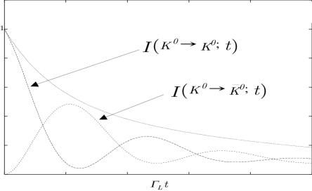
Figure 1: The probabilities of finding a $K^{0}$ and a $\bar{K}^{0}$ in an initial $K^{0}$ beam as a function of time.

These predictions given by Gell-Mann and Pais first assuming C conservation and relaxing it later to CP symmetry were verified experimentally with impressive numerical sensitivity [95]:

$$\Delta M_{K}\equiv M_{K_{L}}-M_{K_{S}}=(3.483\pm 0.006)\cdot 10^{-12}\;{\rm MeV}$$ (41)

(English speakers can rely on a simple mnemonic to remember which state is heavier: ‘L’ stands for larger mass and longer lifetime, whereas ‘S’ denotes smaller and shorter.) This number is a striking demonstration for the sensitivity reached when quantum mechanical interference can be tracked over macroscopic distances, i.e. flight paths of meters or even hundreds of meters. Using the kaon mass as yardstick one can re-express Eq.(41)

$$\frac{\Delta M_{K}}{M_{K}}=\frac{M_{K_{L}}-M_{K_{S}}}{M_{K}}=7.7\cdot 10^{-15}\;,$$ (42)

which is obviously a most striking number. A hard-nosed reader can point out that Eq.(42) vastly overstates the point since the kaon mass generated largely by the strong interactions has no intrinsic connection with $\Delta M_{K}$ generated by the weak interactions and that calibrating $\Delta M_{K}$ by, say, the mass of an elephant is not truly more absurd.

The more relevant yardstick for the oscillation rates is indeed provided by the weak decay rate [95]

$$x_{K} = \frac{\rm oscillation\;rate}{\rm decay\;rate}=\frac{\Delta M_{K}}{\bar{\Gamma}_{K}}\simeq 0.945\pm 0.003$$ (43)

$$y_{K} = \frac{\Delta\Gamma_{K}}{2\bar{\Gamma}_{K}}\simeq 0.996\;\;\;\;{\rm with}\;\;\bar{\Gamma}_{K}=\frac{1}{2}(\Gamma_{K_{S}}+\Gamma_{K_{L}})$$ (44)

The Shock of 1964 – CP Violation Surfaces

1964 was an excellent year for high energy physics: (i) The Higgs mechanism for the ‘spontaneous realization’ of a symmetry was first developed. (ii) The quark model (and the first elements of current algebra) were first suggested. (iii) The charm quark was first introduced to implement quark-lepton symmetry. (iv) The nonrelativistic $SU(6)$ symmetry combining $SU(3)_{Fl}$ with the spin $SU(2)$ was proposed for hadron spectroscopy. (v) The first $e^{+}e^{-}$ storage ring was inaugurated in Frascati. (vi) The $\Omega^{-}$ baryon was found at Brookhaven National Lab, which was viewed as essential validation for the ‘Eightful Way’ of $SU(3)_{Fl}$ symmetry. The modern perspective on it has changed: Being composed of three strange quarks it exhibits rather directly the need for colour as a new internal degree of freedom – together with other observables like $R$ and $\Gamma(\pi^{0}\to 2\gamma)$ as already mentioned in Sect.0.1.1. (vii) CP violation was discovered at the same lab through the observation that $K_{L}$ mesons can decay both into three and two pion final states, albeit the latter with the tiny branching ratio of $0.23\%$ only.

The theoretical concepts listed under items (i) - (iii) and the experimental tool of item (v) turn out to be crucial for the subject matter of these lectures.

It is a fact of life that if one wants to see what moves physicists, one should not focus on what they say (rarely a good indicator for scientists in general), but on what they do. Point in case: How much this discovery shook the HEP community is best gauged by noting the efforts made to reconcile the observation of $K_{L}\to\pi^{+}\pi^{-}$ with CP invariance:

• To infer that $K_{L}\to\pi\pi$ implies CP violation one has to invoke the superposition principle of quantum mechanics. One can introduce [ROOS] nonlinear terms into the Schrödinger equation in such a way as to allow $K_{L}\to\pi^{+}\pi^{-}$ with CP invariant dynamics. While completely ad hoc, it is possible in principle. Such efforts were ruled out by further data, most decisively by $\Gamma(K^{0}(t)\to\pi^{+}\pi^{-})\neq\Gamma(\bar{K}^{0}(t)\to\pi^{+}\pi^{-})$.

• One can try to emulate the success of Pauli’s neutrino hypothesis. An apparent violation of energy-momentum conservation had been observed in $\beta$ decay $n\to pe^{-}$, since the electron exhibited a continuous momentum spectrum. Pauli postulated that the reaction actually was

  $$n\to pe^{-}\bar{\nu}$$ (45)

  with $\bar{\nu}$ a neutral and light particle that had escaped direct observation, yet led to a continuous spectrum for the electron. I.e., Pauli postulated a new particle – and a most whimsical one at that – to save a symmetry, namely the one under translations in space and time responsible for the conservation of energy and momentum. Likewise it was suggested that the real reaction was

  $$K_{L}\to\pi^{+}\pi^{-}U$$ (46)

  with $U$ a neutral and light particle with odd intrinsic CP parity. I.e., a hitherto unseen particle was introduced to save a symmetry. This attempt at evasion was also soon rejected experimentally (see Homework # 1). This represents an example of the ancient Roman saying:

  "Quod licet Jovi, non licet bovi."

  "What is allowed Jupiter, is not allowed a bull."

  I.e., we mere mortals cannot get away with speculations like ‘Jupiter’ Pauli.

Homework # 1

What was the conclusive argument to rule out the reaction of Eq.(46) taking place even for a very tiny $U$ mass?

End of Homework # 1

Notwithstanding these attempts at evasion, the finding of the Fitch-Cronin experiment – namely that $K_{L}\to\pi^{+}\pi^{-}$ does occur – were soon widely accepted, since, in the words of Pram Pais the ‘perpetrators’ were considered ‘real pros’. Yet they induced a feeling of a certain frustration. Parity emerged as violated ‘maximally’ in the charged weak currents that involve left-handed, but no right-handed neutrinos; thus it followed Luther’s dictum "Peccate Fortiter!", i.e. "Sin boldly!". In contrast CP violation, while having an even more profound impact on nature’s basic design as indicated above, appeared as a ‘near-miss’ as suggested by the rarity of the observed transition: BR$(K_{L}\to\pi^{+}\pi^{-})\simeq 0.0023$. Actually we do not know how to give a an unambiguous definition of ‘maximal’ CP violation, as explained in Sect. 0.1.4.

From the discovery in 1964 till the 1973 Kobayashi-Maskawa paper there was no theory of CP violation. Worse still, it was not even recognized – apart from a short remark in a paper by Mohapatra – that the dynamics known at that time were insufficient to implement CP violation. It should be noted that Wolfenstein’s ‘Superweak Model’, which will be sketched below, is not a theory, not even a model – it is a classification scheme, not more and not less.

Yet despite the lack of a true theoretical underpinning, the relevant phenomenology was quickly developed.

Phenomenology of CP Violation, Part I

The discussion here will be given in terms of strangeness $S$, yet can be generalized to any other flavour quantum number $F$ like beauty, charm, etc.

Weak dynamics can drive $\Delta S=1\&2$ transitions, i.e. decays and oscillations. While the underlying theory has to account for both, it is useful to differentiate between them on the phenomenological level. The interplay between $\Delta S=1\&2$ affects also CP violation and how it can manifest itself. Consider $K_{L}\to\pi\pi$: while $\Delta S=2$ dynamics transform the the flavour eigenstates $K^{0}$ and $\bar{K}^{0}$ into mass eigenstates $K_{L}$ and $K_{S}$, $\Delta S=1$ forces produce the decays into pions.

$$[K^{0}\stackrel{{\scriptstyle\Delta S=2}}{{\longleftrightarrow}}\bar{K}^{0}]\Rightarrow K_{L}\stackrel{{\scriptstyle\Delta S=1}}{{\longrightarrow}}\pi\pi$$ (47)

Both of these reactions can exhibit CP violation, which is usually expressed as follows:

$$\eta_{+-[00]} \equiv \frac{T(K_{L}\to\pi^{+}\pi^{-}[\pi^{0}\pi^{0}])}{T(K_{S}\to\pi^{+}\pi^{-}[\pi^{0}\pi^{0}])}$$

$$\eta_{+-} \equiv \epsilon_{K}+\epsilon^{\prime}\;,\;\;\;\eta_{00}\equiv\epsilon_{K}-2\epsilon^{\prime}$$ (48)

Both $\eta_{+-},\eta_{00}\neq 0$ signal CP violation; $\epsilon_{K}$ is common to both observables and reflects the CP properties of the state mixing, i.e. in $\Delta S=2$ dynamics; $\epsilon^{\prime}$ on the other hand differentiates between the two final states and parametrizes CP violation in $\Delta S=1$ dynamics. With an obvious lack in Shakespearean flourish $\epsilon_{K}\neq 0$ is referred to as ‘indirect’ or ‘superweak’ CP violation and $\epsilon^{\prime}\neq 0$ as ‘direct’ CP violation. As long as CP violation is seen only through a single mode of a neutral meson – in this case either $K_{L}\to\pi^{+}\pi^{-}$ or $K_{L}\to\pi^{0}\pi^{0}$ – the distinction between direct and indirect CP violation is somewhat arbitrary, as explained later for $B_{d}$ decays.

Five types of CP violating observables have emerged through $K^{0}-\bar{K}^{0}$ oscillations:

1. Existence of a transition: $K_{L}\to\pi^{+}\pi^{-},\,\pi^{0}\pi^{0}$;

2. An asymmetry due to the initial state: $K^{0}\to\pi^{+}\pi^{-}$ vs. $\bar{K}^{0}\to\pi^{+}\pi^{-}$;

3. An asymmetry due to the final state: $K_{L}\to l^{+}\nu\pi^{-}$ vs. $K_{L}\to l^{-}\bar{\nu}\pi^{+}$, $K_{L}\to\pi^{+}\pi^{-}$ vs. $K_{L}\to\pi^{0}\pi^{0}$;

4. A microscopic T asymmetry: rate$(K^{0}\to\bar{K}^{0})$ $\neq$ rate$(\bar{K}^{0}\to K^{0})$;

5. A T odd correlation in the final state: $K_{L}\to\pi^{+}\pi^{-}e^{+}e^{-}$.

We know now that all these observables except $|\eta_{+-}|\neq|\eta_{00}|$ are predominantly (or even exclusively) given by $\epsilon_{K}$, i.e. indirect CP violation. The asymmetry in semileptonic $K_{L}$ decays has been measured to be

$$\delta_{l}\equiv\frac{\Gamma(K_{L}\rightarrow l^{+}\nu\pi^{-})-\Gamma(K_{L}\rightarrow l^{-}\bar{\nu}\pi^{+})}{\Gamma(K_{L}\rightarrow l^{+}\nu\pi^{-})+\Gamma(K_{L}\rightarrow l^{-}\bar{\nu}\pi^{+})}=(3.27\pm 0.12)\cdot 10^{-3}\;,$$ (49)

averaged over electrons and muons. This measurement provides a convention independent definition of "+" vs. "-", hence of "matter" – $l^{-}$ – vs. "antimatter" – $l^{+}$ – and of "left" – $l^{-}_{L}$ – vs. "right" – $l^{+}_{R}$.

To describe oscillations in the presence of CP violation one turns to solving a nonrelativistic Schrödinger equation, which I formulate for the general case of a pair of neutral mesons $P^{0}$ and $\bar{P}^{0}$ with flavour quantum number $F$; it can denote a $K^{0}$, $D^{0}$ or $B^{0}$ [10]:

$$i\frac{d}{dt}\left(\begin{array}[]{ll}P^{0}\\ \bar{P}^{0}\end{array}\right)=\left(\begin{array}[]{ll}M_{11}-\frac{i}{2}\Gamma_{11}&M_{12}-\frac{i}{2}\Gamma_{12}\\ M^{*}_{12}-\frac{i}{2}\Gamma^{*}_{12}&M_{22}-\frac{i}{2}\Gamma_{22}\end{array}\right)\left(\begin{array}[]{ll}P^{0}\\ \bar{P}^{0}\end{array}\right)$$ (50)

CPT  invariance imposes

$$M_{11}=M_{22}\;\;,\;\;\Gamma_{11}=\Gamma_{22}\;.$$ (51)

Homework # 2:

Which physical situation is described by an equation analogous to Eq.(50) where however the two diagonal matrix elements differ without violating CPT?

End of Homework # 2

The subsequent discussion might strike the reader as overly technical, yet I hope she or he will bear with me since these remarks will lay important groundwork for a proper understanding of CP asymmetries in $B$ decays as well.

The mass eigenstates obtained through diagonalising this matrix are given by (for details see [LEE, BOOK])

$$|P_{A}\rangle = \frac{1}{\sqrt{|p|^{2}+|q|^{2}}}\left(p|P^{0}\rangle+q|\bar{P}^{0}\rangle\right)$$ (52)

$$|P_{B}\rangle = \frac{1}{\sqrt{|p|^{2}+|q|^{2}}}\left(p|P^{0}\rangle-q|\bar{P}^{0}\rangle\right)$$ (53)

with eigenvalues

$$M_{A}-\frac{i}{2}\Gamma_{A} = M_{11}-\frac{i}{2}\Gamma_{11}+\frac{q}{p}\left(M_{12}-\frac{i}{2}\Gamma_{12}\right)$$ (54)

$$M_{B}-\frac{i}{2}\Gamma_{B} = M_{11}-\frac{i}{2}\Gamma_{11}-\frac{q}{p}\left(M_{12}-\frac{i}{2}\Gamma_{12}\right)$$ (55)

as long as

$$\left(\frac{q}{p}\right)^{2}=\frac{M_{12}^{*}-\frac{i}{2}\Gamma^{*}_{12}}{M_{12}-\frac{i}{2}\Gamma_{12}}$$ (56)

holds. I am using letter subscripts $A$ and $B$ for labeling the mass eigenstates rather than numbers $1$ and $2$ as it is usually done. For I want to avoid confusing them with the matrix indices $1,2$ in $M_{ij}-\frac{i}{2}\Gamma_{ij}$.

Eqs.(55) yield for the differences in mass and width

$$\Delta M \equiv M_{B}-M_{A}=-2{\rm Re}\left[\frac{q}{p}(M_{12}-\frac{i}{2}\Gamma_{12})\right]$$ (57)

$$\Delta\Gamma \equiv \Gamma_{A}-\Gamma_{B}=-2{\rm Im}\left[\frac{q}{p}(M_{12}-\frac{i}{2}\Gamma_{12})\right]$$ (58)

Note that the subscripts $A$, $B$ have been swapped in going from $\Delta M$ to $\Delta\Gamma$! This is done to have both quantities positive for kaons.

In expressing the mass eigenstates $P_{A}$ and $P_{B}$ explicitely in terms of the flavour eigenstates – Eqs.(53) – one needs $\frac{q}{p}$. There are two solutions to Eq.(56):

$$\frac{q}{p}=\pm\sqrt{\frac{M_{12}^{*}-\frac{i}{2}\Gamma_{12}^{*}}{M_{12}-\frac{i}{2}\Gamma_{12}}}$$ (59)

There is actually a more general ambiguity than this binary one. For antiparticles are defined up to a phase only:

$${\bf CP}|P^{0}\rangle=\eta|\bar{P}^{0}\rangle\;\;\;{\rm with}\;\;|\eta|=1$$ (60)

Adopting a different phase convention will change the phase for $M_{12}-\frac{i}{2}\Gamma_{12}$ as well as for $q/p$:

$$|\bar{P}^{0}\rangle\rightarrow e^{i\xi}|\bar{P}^{0}\rangle\;\Longrightarrow\;(M_{12},\Gamma_{12})\rightarrow e^{i\xi}(M_{12},\Gamma_{12})\;\&\;\frac{q}{p}\rightarrow e^{-i\xi}\frac{q}{p}\;,$$ (61)

yet leave $(q/p)(M_{12}-\frac{i}{2}\Gamma_{12})$ invariant – as it has to be since the eigenvalues, which are observables, depend on this combination, see Eq.(55). Also $\left|\frac{q}{p}\right|$ is an observable; its deviation from unity is one measure of CP violation in $\Delta F=2$ dynamics.

By convention most authors pick the positive sign in Eq.(59)

$$\frac{q}{p}=+\sqrt{\frac{M_{12}^{*}-\frac{i}{2}\Gamma_{12}^{*}}{M_{12}-\frac{i}{2}\Gamma_{12}}}\;.$$ (62)

Up to this point the two states $|P_{A,B}\rangle$ are merely labelled by their subscripts. Indeed $|P_{A}\rangle$ and $|P_{B}\rangle$ switch places when selecting the minus rather than the plus sign in Eq.(59).

One can define the labels $A$ and $B$ such that

$$\Delta M\equiv M_{B}-M_{A}>0$$ (63)

is satisfied. Once this convention has been adopted, it becomes a sensible question whether

$$\Gamma_{B}>\Gamma_{A}\;\;\;{\rm or}\;\;\;\Gamma_{B}<\Gamma_{A}$$ (64)

holds, i.e. whether the heavier state is shorter or longer lived.

One can write the general mass eigenstates in terms of the CP eigenstates as well:

$$|P_{A}\rangle = \frac{1}{\sqrt{1+|\bar{\epsilon}|^{2}}}\left(|P_{+}\rangle+\bar{\epsilon}|P_{-}\rangle\rangle\right)\;\;\;,\;CP|P_{\pm}\rangle=\pm|P_{\pm}\rangle$$ (65)

$$|P_{B}\rangle = \frac{1}{\sqrt{1+|\bar{\epsilon}|^{2}}}\left(|P_{-}\rangle+\bar{\epsilon}|P_{+}\rangle\rangle\right)\;;$$ (66)

$\bar{\epsilon}=0$ means that the mass and CP eigenstates coincide, i.e. CP is conserved in $\Delta F=2$ dynamics driving $P-\bar{P}$ oscillations. With the phase between the orthogonal states $|P_{+}\rangle$ and $|P_{-}\rangle$ arbitrary, the phase of $\bar{\epsilon}$ can be changed at will and is not an observable; $\bar{\epsilon}$ can be expressed in terms of $\frac{q}{p}$, yet in a way that depends on the convention for the phase of antiparticles. For ${\bf CP}|P\rangle=\pm|\bar{P}\rangle$ one has

$$|P_{+}\rangle = \frac{1}{\sqrt{2}}\left(|P^{0}\rangle\pm|\bar{P}^{0}\rangle\right)$$ (67)

$$|P_{-}\rangle = \frac{1}{\sqrt{2}}\left(|P^{0}\rangle\mp|\bar{P}^{0}\rangle\right)$$ (68)

$$\bar{\epsilon} = \frac{1\mp\frac{q}{p}}{1\pm\frac{q}{p}}$$ (69)

Homework # 3:

While $\langle\bar{P}^{0}|P^{0}\rangle=0$ holds – e.g., $\langle\bar{K}^{0}|K^{0}\rangle=0$ –, one has $\langle K_{L}|K_{S}\rangle\neq 0$ and in general $\langle P_{B}|P_{A}\rangle\neq 0$. Calculate it and interprete your result.

End of Homework # 3

Later we will discuss how to evaluate $M_{12}$ and thus also $\Delta M$ within a given theory for the $P-\bar{P}$ complex. The examples just listed illustrate that some care has to be applied in interpreting such results. For expressing mass eigenstates explicitely in terms of flavour eigenstates involves some conventions. Once adopted we have to stick with a convention; yet our original choice cannot influence observables.

Let me recapitulate the relevant points:

• The labels of the two mass eigenstates $P_{A}$ and $P_{B}$ can be chosen such that

  $$M_{P_{B}}>M_{P_{A}}$$ (70)

  holds.

• Then it becomes an empirical question whether $P_{A}$ or $P_{B}$ are longer lived:

  $$\Gamma_{P_{A}}>\Gamma_{P_{B}}\;\;\;{\rm or}\;\;\;\Gamma_{P_{A}}<\Gamma_{P_{B}}\;\;?$$ (71)

• In the limit of CP invariance one can also raise the question whether it is the CP even or the odd state that is heavier.

• We will see later that within a given theory for $\Delta F=2$ dynamics one can calculate $M_{12}$, including its sign, if phase conventions are treated consistently. To be more specific: adopting a phase convention for $\frac{q}{p}$ and having ${\cal L}(\Delta F=2)$ one can calculate $\frac{q}{p}\left(M_{12}-\frac{i}{2}\Gamma_{12}\right)=\frac{q}{p}\langle P^{0}|{\cal L}(\Delta F=2)|\bar{P}^{0}\rangle$. Then one assigns the labels $B$ and $A$ such that $\Delta M=M_{B}-M_{A}=-2{\rm Re}\frac{q}{p}\left(M_{12}-\frac{i}{2}\Gamma_{12}\right)$ turns out to be positive!

0.1.6 CKM – From a General Ansatz to a Specific Theory

Electroweak forces can be dealt with perturbatively. Consider the $\Delta S=1$ four-fermion transition operator: $(\bar{u}_{L}\gamma^{\mu}s_{L})(\bar{d}_{L}\gamma_{\mu}u_{L})$. It constitutes a dimension-six operator. Yet placing such an operator – or any other operator with dimension larger than four – into the Lagrangian creates nonrenormalizable interactions. What happened is that we have started out from a renormalizable Lagrangian

$${\cal L}_{CC}=g_{W}\bar{q}^{(i)}_{L}\gamma_{\mu}q_{L}^{(j)}W^{\mu}\;,$$ (72)

iterated it to second order in $g_{W}$ with $(q^{(i)},q^{(j)})=(u,s)\&(u,d)$ and then ‘integrated out’ the heavy field, namely in this case the vector boson field $W^{\mu}$. That way one arrives at an effective Lagrangian containing only light quarks as ‘active’ fields.

Such effective field theories have experienced a veritable renaissance in the last ten years. Constructing them in a self-consistent way is greatly helped by adopting a Wilsonian prescription:

• First one defines a field theory ${\cal L}(\Lambda_{UV})$ at a high ultraviolet scale $\Lambda_{UV}\gg$ germane scales of theory like $M_{W}$, $m_{Q}$ etc.

• For applications characterized by physical scales $\Lambda_{phys}$ one renormalizes the theory from the cutoff $\Lambda_{UV}$ down to $\Lambda_{phys}$. In doing so one integrates out the heavy degrees of freedom, i.e. with masses exceeding $\Lambda_{phys}$ – like $M_{W}$ – to arrive at an effective low energy field theory using the operator product expansion (OPE) as a tool:

  $${\cal L}(\Lambda_{UV})\Rightarrow{\cal L}(\Lambda_{phys})=\sum_{i}c_{i}(\Lambda_{phys},\Lambda_{UV},M_{W},...){\cal O}_{i}(\Lambda_{phys})$$ (73)

  • The local operators ${\cal O}_{i}(\Lambda_{phys})$ contain the active dynamical fields, i.e. those with frequencies below ${\cal O}_{i}(\Lambda_{phys})$.

  • Their c number coefficients $c_{i}(\Lambda_{phys},\Lambda_{UV},M_{W},...)$ provide the gateway for heavy degrees of freedom with frequencies exceeding ${\cal O}_{i}(\Lambda_{phys})$ to enter. They are shaped by short-distance dynamics and therefore usually computed perturbatively.

• Lowering the value of ${\cal O}_{i}(\Lambda_{phys})$ in general changes the form of the Lagrangian: ${\cal L}(\Lambda^{(1)}_{phys})\neq{\cal L}(\Lambda^{(2)}_{phys})$ for $\Lambda^{(1)}_{phys}\neq\Lambda^{(2)}_{phys}$. In particular integrating out heavy degrees of freedom will induce higher-dimensional operators to emerge in the Lagrangian. In the example above integrating the $W$ field from the dimension-four term in Eq.(72) produces dimension six four-quark operators.

• As a matter of principle observables cannot depend on the choice of $\Lambda_{phys}$; the latter primarily provides just a demarkation line:

  $${\rm short\;distances}<1/\Lambda_{phys}<{\rm long\;distances}$$ (74)

In practice, however, its value must be chosen judiciously due to limitations of our (present) computational abilities: on one hand we want to be able to calculate radiative corrections perturbatively and thus require $\alpha_{S}(\Lambda_{phys})<1$. Taken by itself it would suggest to choose $\Lambda_{phys}$ as large as possible. Yet on the other hand we have to evaluate hadronic matrix elements; there $\Lambda_{phys}$ can provide an UV cutoff on the momenta of the hadronic constituents. Since the tails of hadronic wave functions cannot be obtained from, say, quark models in a reliable way, one wants to pick $\Lambda_{phys}$ as low as possible. More specifically for heavy flavour hadrons one can expand their matrix elements in powers of $\Lambda_{phys}/m_{Q}$. Thus one encounters a Scylla & Charybdis situation. A reasonable middle course can be steered by picking $\Lambda_{phys}\sim 1$ GeV, and hence I will denote this quantity and this value by $\mu$.

Some concrete examples might illuminate these remarks.

• Iterating the coupling of Eq.(72) leads to an effective current-current coupling $(\bar{u}_{L}\gamma^{\mu}s_{L})(\bar{d}_{L}\gamma_{\mu}u_{L})$ at low energies, i.e. scales below $M_{W}$. QCD radiative corrections have to be included: they affect the strength of these effective weak transition operators significantly, since they represent an expansion in $\alpha_{S}$ multiplied by a numerically large logarithm log$(M_{W}/\mu)$ rather than merely $\alpha_{S}$; they also create different types of such operators. On the tree graph level there is one $\Delta S=1$ operator, namely $(\bar{u}_{L}\gamma_{\mu}s_{L})(\bar{d}_{L}\gamma^{\mu}u_{L})$. Including one-loop diagrams where a gluon is exchanged between quark lines one obtains ${\cal O}(\alpha_{S})$ contributions to the original $(\bar{u}_{L}\gamma_{\mu}s_{L})(\bar{d}_{L}\gamma^{\mu}u_{L})$ operator – and to the new coupling $(\bar{u}_{L}\gamma_{\mu}t^{i}s_{L})(\bar{d}_{L}\gamma^{\mu}t^{i}u_{L})$, where the $t^{i}$ denote the generators of colour $SU(3)$. I.e., the two operators $O^{1\times 1}=(\bar{u}_{L}\gamma_{\mu}s_{L})(\bar{d}_{L}\gamma^{\mu}u_{L})$ and $O^{8\times 8}=(\bar{u}_{L}\gamma_{\mu}t^{i}s_{L})(\bar{d}_{L}\gamma^{\mu}t^{i}u_{L})$, where the former [latter] represents the product of two colour-singlet[octet] currents, mix under QCD renormalization already on the one-loop level:

  $$(\bar{u}_{L}\gamma_{\mu}s_{L})(\bar{d}_{L}\gamma^{\mu}u_{L})\;\;\;\stackrel{{\scriptstyle{\rm QCD\,1-loop\,renormalization}}}{{\Longrightarrow}}\;\;\;c_{1\times 1}O^{1\times 1}+c_{8\times 8}O^{8\times 8}$$ (75)

  with $c_{1\times 1}=1+{\cal O}(\alpha_{S})$, whereas $c_{8\times 8}={\cal O}(\alpha_{S})$. Since some of these $\alpha_{S}$ corrections are actually enhanced by numerically sizeable log$(M_{W}/\mu)$ factors, they are quite significant. Therefore one wants to identify the multiplicatively renormalized transition operators with

  $$\tilde{O}\;\;\;\;\;\stackrel{{\scriptstyle{\rm QCD\,1-loop\,renormalization}}}{{\Longrightarrow}}\;\;\;\;\;\tilde{c}\;\tilde{O}$$ (76)

  This can be done even without brute-force computations by relying on isospin arguments: consider the weak scattering process between quarks

  $$s_{L}+u_{L}\to u_{L}+d_{L}$$ (77)

  proceeding in an S wave. It can be driven by two $\Delta S=1$ operators, namely

  $$O_{\pm}=\frac{1}{2}\left[(\bar{u}_{L}\gamma_{\mu}s_{L})(\bar{d}_{L}\gamma^{\mu}u_{L})\pm(\bar{d}_{L}\gamma_{\mu}s_{L})(\bar{u}_{L}\gamma^{\mu}u_{L})\right]$$ (78)

  The operator $O_{+}[O_{-}]$ produces an $ud$ pair in the final state that is [anti]symmetric in isospin and thus carries $I=1[I=0]$; since the initial $su$ pair carries $I=1/2$, $O_{+}[O_{-}]$ generates $\Delta I=1/2\&3/2$ [only $\Delta I=1/2]$ transitions.

  With QCD conserving isospin, its radiative corrections cannot mix the operators $O_{\pm}$, which therefore are multiplicatively renormalized:

  $$O_{+}\;[O_{-}]\;\;\;\;\;\stackrel{{\scriptstyle{\rm QCD\,1-loop\,renormalization}}}{{\Longrightarrow}}\;\;\;\;\;c_{+}\,O_{+}\;[c_{-}\,O_{-}]\;.$$ (79)

  and therefore

  $${\cal L}_{eff}^{(0)}(\Delta S=1)=O_{+}+O_{-}\;\;\;\stackrel{{\scriptstyle{\rm QCD\,1-loop\,ren.}}}{{\Longrightarrow}}\;\;\;{\cal L}_{eff}(\Delta S=1)=c_{+}\,O_{+}+c_{-}\,O_{-}$$ (80)

  with $c_{\pm}=1+{\cal O}(\alpha_{S})$.

  Integrating out those loops containing a $W$ line in addition to the gluon line and two quark lines yields terms $\propto\alpha_{S}{\rm log}(M_{W}^{2}/\mu^{2})$, which are not necessarily small. Using the renormalization group equation to sum those terms terms one finds on the leading log level

  $$c_{\pm}=\left[\frac{\alpha_{S}(M_{W}^{2})}{\alpha_{S}(\mu^{2})}\right]^{\gamma_{\pm}}\;,\;\;\gamma_{+}=\frac{6}{33-2N_{F}}=-\frac{1}{2}\gamma_{-}\;.$$ (81)

  I.e.,

  $$c_{-}>1>c_{+}\;,\;\;c_{-}c_{+}^{2}=1$$ (82)

  That means that QCD radiative corrections provide a quite sizeable $\Delta I=1/2$ enhancement. Corresponding effects arise for ${\cal L}_{eff}(\Delta C/B=1)$.

  QCD radiative corrections create yet another effect, namely they lead to the emergence of ‘Penguin’ operators. Without the gluon line their diagram would decompose into two disconnected parts and thus not contribute to a transition operator. These Penguin diagrams can drive only $\Delta I=1/2$ modes. Furthermore in the loop all three quark families contribute; the diagram thus contains the irreducible CKM phase – i.e. it generates direct CP violation in strange decays. Similar effects arise in beauty, but not necessarily in charm decays.

• Consider $K^{0}-\bar{K}^{0}$ oscillations, which represent $\Delta S=2$ transitions. As explained in Sect.0.1.5 those are driven by the off-diagonal elements of a ‘generalized mass matrix’:

  $${\cal M}_{12}=M_{12}+\frac{i}{2}{\Gamma}_{12}=\langle K^{0}|{\cal L}_{eff}(\Delta S=2)|\bar{K}^{0}\rangle$$ (83)

  The observables $\Delta M_{K}$ and $\epsilon_{K}$ are given in terms of Re$M_{12}$ and Im$M_{12}$, respectively. In the SM ${\cal L}_{eff}(\Delta S=2)$, which generates $M_{12}$, is produced by iterating two $\Delta S=1$ operators:

  $${\cal L}_{eff}(\Delta S=2)={\cal L}(\Delta S=1)\otimes{\cal L}(\Delta S=1)$$ (84)

  This leads to the well known quark box diagrams, which generate a local $\Delta S=2$ operator. The contributions that do not depend on the mass of the internal quarks cancel against each other due to the GIM mechanism, which leads to highly convergent diagrams. Integrating over the internal fields, namely the $W$ bosons and the top and charm quarks then yields a convergent result:

  $${\cal L}_{eff}^{box}(\Delta S=2,\mu)=\left(\frac{G_{F}}{4\pi}\right)^{2}\cdot$$

  $$\left[\xi_{c}^{2}E(x_{c})\eta_{cc}+\xi_{t}^{2}E(x_{t})\eta_{tt}+2\xi_{c}\xi_{t}E(x_{c},x_{t})\eta_{ct}\right][\alpha_{S}(\mu^{2})]^{-\frac{6}{27}}\left(\bar{d}\gamma_{\mu}(1-\gamma_{5})s\right)^{2}+h.c.$$ (85)

  with $\xi_{i}$ denoting combinations of KM parameters

  $$\xi_{i}=V(is)V^{*}(id)\;,\;\;i=c,t\;;$$ (86)

  $E(x_{i})$ and $E(x_{c},x_{t})$ reflect the box loops with equal and different internal quarks, respectively [INAMI]:

  $$E(x_{i})=x_{i}\left(\frac{1}{4}+\frac{9}{4(1-x_{i})}-\frac{3}{2(1-x_{i})^{2}}\right)-\frac{3}{2}\left(\frac{x_{i}}{1-x_{i}}\right)^{3}{\rm log}x_{i}$$ (87)

  $$E(x_{c},x_{t})=x_{c}x_{t}\left[\left(\frac{1}{4}+\frac{3}{2(1-x_{t})}-\frac{3}{4(1-x_{t})^{2}}\right)\frac{{\rm log}x_{t}}{x_{t}-x_{c}}+(x_{c}\leftrightarrow x_{t})-\right.$$

  $$\left.-\frac{3}{4}\frac{1}{(1-x_{c})(1-x_{t})}\right]$$ (88)

  $$x_{i}=\frac{m_{i}^{2}}{M_{W}^{2}}\;.$$ (89)

  The $\eta_{ij}$ represent the QCD radiative corrections from evolving the effective Lagrangian from $M_{W}$ down to the internal quark mass. The factor $[\alpha_{S}(\mu^{2})]^{-6/27}$ reflects the fact that a scale $\mu$ must be introduced at which the four-quark operator $\left(\bar{s}\gamma_{\mu}(1-\gamma_{5})d\right)^{2}$ is defined. This dependance on the auxiliary variable $\mu$ drops out when one takes the matrix element of this operator (at least when one does it correctly). Including next-to-leading log corrections one finds (for $m_{t}\simeq 180$ GeV) [BURAS]:

  $$\eta_{cc}\simeq 1.38\pm 0.20\;,\;\;\eta_{tt}\simeq 0.57\pm 0.01\;,\;\;\eta_{cc}\simeq 0.47\pm 0.04$$ (90)

  The dominant contributions for $\Delta M(K)$ and $\epsilon_{K}$ are produced, when (in addition to the $W^{\pm}$ pair) the internal quarks are charm and top, respectively. In either case the internal quarks are heavier than the external ones: $m_{d},m_{s}\ll m_{c},m_{t}$, and evaluating the Feynman diagrams indeed corresponds to integrating out the heavy fields.

  The situation is qualitatively very similar for $\Delta M(B^{0})$, and in some sense even simpler: for within the SM by far the leading contribution is due to internal top quarks. Evaluating the quark box diagram with internal $W$ and top quark lines corresponds to integrating those heavy degrees of freedom out in a straightforward way leading to:

  $${\cal L}_{eff}^{box}(\Delta B=2,\mu)\simeq\left(\frac{G_{F}}{4\pi}\right)^{2}M_{W}^{2}\cdot\xi_{t}^{2}E(x_{t})\eta_{tt}\left(\bar{q}\gamma_{\mu}(1-\gamma_{5})b\right)^{2}+h.c.$$ (91)

  with $q=d,s$.

  Homework # 4

  When one calculates $\Delta M(B)$ as a function of the top mass employing the quark box diagram, one finds, see Eq.(87)

  $$\Delta M(B)\propto\left(\frac{m_{t}}{M_{W}}\right)^{2}\;\;{\rm for}\;\;m_{t}\gg M_{W}$$ (92)

  The factor on the right hand side reflects the familiar GIM suppression for $m_{t}\ll M_{W}$; yet for $m_{t}\gg M_{W}$ it constitutes a (huge) enhancement! It means that a low energy observable, namely $\Delta M(B)$, is controlled more and more by a state or field at asymptotically high scales. Does this not violate decoupling theorems and even common sense? Does it violate decoupling – and if so, why is it allowed to do so – or not?

  End of Homework # 4

  While quark box diagrams contribute also to $\Gamma_{12}(\Delta S=2)$, it would be absurd to assume they are significant. For $\Gamma_{K}$ is dominated by the impact of hadronic phase space causing $\Gamma(K_{neut}\to 2\pi)\gg\Gamma(K_{neut}\to 3\pi)$. Yet even beyond that it is unlikely that such a computation would make much sense: to contribute to $\Delta\Gamma_{K}$ the internal quark lines in the quark box diagram have to be $u$ and $\bar{u}$ quarks, i.e. lighter than the external quarks $s$ and $\bar{s}$. That means calculating this Feynman diagram does not correspond to integrating out the heavy degrees of freedom. For the same reason (and others as explained later in more detail) computing quark box diagrams tells us little of value concerning $D^{0}-\bar{D}^{0}$ oscillations, since the internal quarks on the leading CKM level – $s$ and $\bar{s}$ – are lighter than the external charm quarks.

  A new and more intriguing twist concerning quark box diagrams occurs when addressing $\Delta\Gamma$ for $B^{0}$ mesons. Those diagrams again do not generate a local operator, since the internal charm quarks carry less than half the mass of the external $b$ quarks. Nevertheless it can be conjectured that the on-shell $\Delta B=2$ transition operator generating $\Delta\Gamma_{B}$ is largely shaped by short distance dynamics.

The main message of these more technical considerations was to show that while QCD conserves flavour, it has a highly nontrivial impact on flavour transitions by not only affecting the strength of the bare weak operator, but also inducing new types of weak transition operators already on the perturbative level. In particular, QCD creates a source of direct CP violation in strange decays naturally, albeit with a significantly reduced strength.

0.1.7 The SM Paradigm of Large CP Violation in $B$ Decays

Basics

As pointed out in Sect.0.1.2 for an observable CP asymmetry to emerge in a decay one needs two different, yet coherent amplitudes to contribute. In 1979 it was pointed out that $B^{0}-\bar{B}^{0}$ oscillations are well suited to satisfy this requirement for final states $f$ that can be fed both by $B^{0}$ and $\bar{B}^{0}$ decays, in particular since those oscillation rates were expected to be sizable [11]:

$$B^{0}\Rightarrow\bar{B}^{0}\to f\leftarrow B^{0}\hskip 28.45274ptvs.\hskip 28.45274pt\bar{B}^{0}\Rightarrow B^{0}\to\bar{f}\leftarrow B^{0}$$ (93)

In 1980 it was predicted [12]that in particular $B_{d}\to\psi K_{S}$ should exhibit such a CP asymmetry larger by two orders of magnitude than the corresponding one in $K^{0}\to 2\pi$ vs. $\bar{K}^{0}\to 2\pi$, if CKM theory provides the main driver of $K_{L}\to\pi^{+}\pi^{-}$; even values close to 100 % were suggested as conceivable. The analogous mode $B_{s}\to\psi\phi$ should however show an asymmetry not exceeding the few percent level.

It was also suggested that in rare modes like $\bar{B}_{d}\to K^{-}\pi^{+}$ sizable direct CP violation could emerge due to intervention of ‘Penguin’ operators [13].

We now know that these predictions were rather prescient. It should be noted that at the time of these predictions very little was known about $B$ mesons. While their existence had been inferred from the discovery of the $\Upsilon(1S-4S)$ family at FNAL in 1977ff, none of their exclusive decays had been identified, and their lifetime were unknown as were a forteriori their oscillation rates. Yet the relevant formalism for CP asymmetries involving $B^{0}-\bar{B}^{0}$ oscillations was already fully given.

Decay rates for CP conjugate channels can be expressed as follows:

$$\begin{array}[]{l}{\rm rate}(B(t)\rightarrow f)=e^{-\Gamma_{B}t}G_{f}(t)\\ {\rm rate}(\bar{B}(t)\rightarrow\bar{f})=e^{-\Gamma_{B}t}\bar{G}_{\bar{f}}(t)\end{array}$$ (94)

where CPT invariance has been invoked to assign the same lifetime $\Gamma_{B}^{-1}$ to $B$ and $\bar{B}$ hadrons. Obviously if

$$\frac{G_{f}(t)}{\bar{G}_{\bar{f}}(t)}\neq 1$$ (95)

is observed, CP violation has been found. Yet one should keep in mind that this can manifest itself in two (or three) qualitatively different ways:

1. $$\frac{G_{f}(t)}{\bar{G}_{\bar{f}}(t)}\neq 1\;\;{\rm with}\;\;\frac{d}{dt}\frac{G_{f}(t)}{\bar{G}_{\bar{f}}(t)}=0\;;$$ (96)

   i.e., the asymmetry is the same for all times of decay. This is true for direct CP violation; yet, as explained later, it also holds for CP violation in the oscillations.

2. $$\frac{G_{f}(t)}{\bar{G}_{\bar{f}}(t)}\neq 1\;\;{\rm with}\;\;\frac{d}{dt}\frac{G_{f}(t)}{\bar{G}_{\bar{f}}(t)}\neq 0\;;$$ (97)

   here the asymmetry varies as a function of the time of decay. This can be referred to as CP violation involving oscillations.

A straightforward application of quantum mechanics with its linear superposition principle yields [1] for $\Delta\Gamma=0$, which holds for $B^{\pm}$ and $\Lambda_{b}$ exactly and for $B_{d}$ to a good approximation :

$$\begin{array}[]{l}G_{f}(t)=|T_{f}|^{2}\left[\left(1+\left|\frac{q}{p}\right|^{2}|\bar{\rho}_{f}|^{2}\right)+\left(1-\left|\frac{q}{p}\right|^{2}|\bar{\rho}_{f}|^{2}\right){\rm cos}\Delta m_{B}t-2({\rm sin}\Delta m_{B}t){\rm Im}\frac{q}{p}\bar{\rho}_{f}\right]\\ \bar{G}_{\bar{f}}(t)=|\bar{T}_{\bar{f}}|^{2}\left[\left(1+\left|\frac{p}{q}\right|^{2}|\rho_{\bar{f}}|^{2}\right)+\left(1-\left|\frac{p}{q}\right|^{2}|\rho_{\bar{f}}|^{2}\right){\rm cos}\Delta m_{B}t-2({\rm sin}\Delta m_{B}t){\rm Im}\frac{p}{q}\rho_{\bar{f}}\right]\end{array}$$ (98)

The amplitudes for the instantaneous $\Delta B=1$ transition into a final state $f$ are denoted by $T_{f}=T(B\rightarrow f)$ and $\bar{T}_{f}=T(\bar{B}\rightarrow f)$ and

$$\bar{\rho}_{f}=\frac{\bar{T}_{f}}{T_{f}}\;\;,\rho_{\bar{f}}=\frac{T_{\bar{f}}}{\bar{T}_{\bar{f}}}\;\;,\frac{q}{p}=\sqrt{\frac{M_{12}^{*}-\frac{i}{2}\Gamma_{12}^{*}}{M_{12}-\frac{i}{2}\Gamma_{12}}}$$ (99)

Staring at the general expression is not always very illuminating; let us therefore consider three limiting cases:

• $\Delta m_{B}=0$, i.e. no $B^{0}-\bar{B}^{0}$ oscillations:

  $$G_{f}(t)=2|T_{f}|^{2}\;\;,\;\;\bar{G}_{\bar{f}}(t)=2|\bar{T}_{\bar{f}}|^{2}\leadsto\frac{\bar{G}_{\bar{f}}(t)}{G_{f}(t)}=\left|\frac{\bar{T}_{\bar{f}}}{T_{f}}\right|^{2}\;\;,\frac{d}{dt}G_{f}(t)\equiv 0\equiv\frac{d}{dt}\bar{G}_{\bar{f}}(t)$$ (100)

  This is explicitely what was referred to above as direct CP violation.

• $\Delta m_{B}\neq 0$ and $f$ a flavour-specific final state with no direct CP violation; i.e., $T_{f}=0=\bar{T}_{\bar{f}}$ and $\bar{T}_{f}=T_{\bar{f}}$ :

  $$\begin{array}[]{c}G_{f}(t)=\left|\frac{q}{p}\right|^{2}|\bar{T}_{f}|^{2}(1-{\rm cos}\Delta m_{B}t)\;\;,\;\;\bar{G}_{\bar{f}}(t)=\left|\frac{p}{q}\right|^{2}|T_{\bar{f}}|^{2}(1-{\rm cos}\Delta m_{B}t)\\ \leadsto\frac{\bar{G}_{\bar{f}}(t)}{G_{f}(t)}=\left|\frac{q}{p}\right|^{4}\;\;,\;\;\frac{d}{dt}\frac{\bar{G}_{\bar{f}}(t)}{G_{f}(t)}\equiv 0\;\;,\;\;\frac{d}{dt}\bar{G}_{\bar{f}}(t)\neq 0\neq\frac{d}{dt}G_{f}(t)\end{array}$$ (101)

  This constitutes CP violation in the oscillations. For the CP conserving decay into the flavour-specific final state is used merely to track the flavour identity of the decaying meson. This situation can therefore be denoted also in the following way:

  $$\frac{{\rm Prob}(B^{0}\Rightarrow\bar{B}^{0};t)-{\rm Prob}(\bar{B}^{0}\Rightarrow B^{0};t)}{{\rm Prob}(B^{0}\Rightarrow\bar{B}^{0};t)+{\rm Prob}(\bar{B}^{0}\Rightarrow B^{0};t)}=\frac{|q/p|^{2}-|p/q|^{2}}{|q/p|^{2}+|p/q|^{2}}=\frac{1-|p/q|^{4}}{1+|p/q|^{4}}$$ (102)

• $\Delta m_{B}\neq 0$ with $f$ now being a flavour-nonspecific final state – a final state common to $B^{0}$ and $\bar{B}^{0}$ decays – of a special nature, namely a CP eigenstate – $|\bar{f}\rangle={\bf CP}|f\rangle=\pm|f\rangle$ – without direct CP violation – $|\bar{\rho}_{f}|=1=|\rho_{\bar{f}}|$:

  $$\begin{array}[]{c}G_{f}(t)=2|T_{f}|^{2}\left[1-({\rm sin}\Delta m_{B}t)\cdot{\rm Im}\frac{q}{p}\bar{\rho}_{f}\right]\\ \bar{G}_{f}(t)=2|T_{f}|^{2}\left[1+({\rm sin}\Delta m_{B}t)\cdot{\rm Im}\frac{q}{p}\bar{\rho}_{f}\right]\\ \leadsto\frac{d}{dt}\frac{\bar{G}_{f}(t)}{G_{f}(t)}\neq 0\\ \frac{\bar{G}_{f}(t)-G_{f}(t)}{\bar{G}_{f}(t)+G_{f}(t)}=({\rm sin}\Delta m_{B}t)\cdot{\rm Im}\frac{q}{p}\bar{\rho}_{f}\end{array}$$ (103)

  is the concrete realization of what was called CP violation involving oscillations.

  For $f$ still denoting a CP eigenstate, yet with $|\bar{\rho}_{f}|\neq 1$ one has the more complex asymmetry expression

  $$\frac{\bar{G}_{f}(t)-G_{f}(t)}{\bar{G}_{f}(t)+G_{f}(t)}=S_{f}\cdot({\rm sin}\Delta m_{B}t)-C_{f}\cdot({\rm cos}\Delta m_{B}t)$$ (104)

  with

  $$S_{f}=\frac{2{\rm Im}\frac{q}{p}\bar{\rho}_{\pi^{+}\pi^{-}}}{1+\left|\frac{q}{p}\bar{\rho}_{\pi^{+}\pi^{-}}\right|^{2}}\;,\;\;C_{f}=\frac{1-\left|\frac{q}{p}\bar{\rho}_{\pi^{+}\pi^{-}}\right|^{2}}{1+\left|\frac{q}{p}\bar{\rho}_{\pi^{+}\pi^{-}}\right|^{2}}$$ (105)

For the decays of neutral mesons the following general statement is relevant, at least conceptually.

Theorem:

Consider a beam with an arbitrary combination of neutral mesons $P^{0}$ and $\bar{P}^{0}$ decaying into a final state $f$ that is a CP eigenstate. If the decay rate evolution in (proper) time $t$ is not described by a single exponential, i.e.

$${\rm rate}(P^{0}/\bar{P}^{0}(t)\to f)\neq Ke^{-\Gamma t}\;\;\;{\rm with}\;\;\;\frac{d}{dt}K\equiv 0$$ (106)

for any real $\Gamma$, then CP invariance is violated.

Homework # 5

Prove this theorem.

End of Homework # 5

An obvious, yet still useful criterion for CP observables is that they must be ‘re-phasing’ invariant under $|\bar{B}^{0}\rangle\to e^{-i\xi}|\bar{B}^{0}\rangle$. The expressions above show there are three classes of such observables:

• An asymmetry in the instantaneous transition amplitudes for CP conjugate modes:

  $$|T(B\to f)|\neq|T(\bar{B}\to\bar{f})|\hskip 28.45274pt\Longleftrightarrow\hskip 28.45274pt\Delta B=1\;.$$ (107)

  It reflects pure $\Delta B=1$ dynamics and thus amounts to direct CP violation. Those modes are most likely to be nonleptonic; in the SM they practically have to be.

• CP violation in $B^{0}-\bar{B}^{0}$ oscillations:

  $$|q|\neq|p|\hskip 28.45274pt\Longleftrightarrow\hskip 28.45274pt\Delta B=2\;.$$ (108)

  It requires CP violation in $\Delta B=2$ dynamics. The theoretically cleanest modes here are semileptonic ones due to the SM $\Delta Q=\Delta B$ selection rule.

• CP asymmetries involving oscillations :

  $${\rm Im}\frac{q}{p}\bar{\rho}(f)\neq 0\;,\;\;\bar{\rho}(f)=\frac{T(\bar{B}\to f)}{T(B\to f)}\hskip 28.45274pt\Longleftrightarrow\hskip 28.45274pt\Delta B=1\&2\;.$$ (109)

  Such an effect requires the interplay of $\Delta B=1\&2$ forces.

  While $C_{f}\neq 0$ unequivocally signals direct CP violation in Eq.(104), the interpretation of $S_{f}\neq 0$ is more complex. (i) As long as one has measured $S_{f}$ only in a single mode, the distinction between direct and indirect CP violation – i.e. CP violation in $\Delta B=1$ and $\Delta B=2$ dynamics – is convention dependent, since a change in phase for $\bar{B}^{0}$ – $|\bar{B}^{0}\rangle\to e^{-i\xi}|\bar{B}^{0}\rangle$ – leads to $\bar{\rho}_{f}\to e^{-i\xi}\bar{\rho}_{f}$ and $(q/p)\to e^{i\xi}(q/p)$, i.e. can shift any phase from $(q/p)$ to $\bar{\rho}_{f}$ and back while leaving $(q/p)\bar{\rho}_{f}$ invariant. However once $S_{f}$ has been measured for two different final states $f$, then the distinction becomes truly meaningful independent of theory: $S_{f_{1}}\neq S_{f_{2}}$ implies $(q/p)\bar{\rho}_{f_{1}}\neq(q/p)\bar{\rho}_{f_{2}}$ and thus $\bar{\rho}_{f_{1}}\neq\bar{\rho}_{f_{2}}$, i.e. CP violation in the $\Delta B=1$ sector. One should note that this direct CP violation might not generate a $C_{f}$ term. For $\bar{\rho}_{f_{1}}=e^{i\phi_{1}}$ and $\bar{\rho}_{f_{2}}=e^{i\phi_{2}}$ causing $S_{f_{1}}\neq S_{f_{2}}$ would both lead to $C_{f_{1}}=0=C_{f_{2}}$.

Once the final state consists of more than two pseudoscalar or one pseudoscalar and one vector meson, it contains more dynamical information than expressed through the decay width into it, as can be described through a Dalitz plot.

• Accordingly one can have a CP asymmetry in final state distributions of $B$ mesons, as discussed later. There is a precedent for such an effect, namely a T odd correlation that has been observed between the $\pi^{+}-\pi^{-}$ and $e^{+}-e^{-}$ planes in the rare mode $K_{L}\to\pi^{+}\pi^{-}e^{+}e^{-}$, the size of which can be inferred from $K_{L}\to\pi^{+}\pi^{-}$.

The First Central Pillar of the Paradigm: Long Lifetimes

Beauty, the existence of which had been telegraphed by the discovery of the $\tau$ as the third charged lepton was indeed observed exhibiting a surprising feature: starting in the early 1980’s its lifetime was found to be about $10^{-12}$ sec. This was considered ‘long’. For one can get an estimate for $\tau(B)$ by relating it to the muon lifetime:

$$\tau(B)\simeq\tau_{b}\sim\tau(\mu)\left(\frac{m(\mu)}{m(b)}\right)^{5}\frac{1}{9}\frac{1}{|V(cb)|^{2}}\simeq 3\cdot 10^{-14}\left|\frac{{\rm sin}\theta_{C}}{V(cb)}\right|^{2}\;{\rm sec}$$ (110)

One had expected $|V(cb)|$ to be suppressed, since it represents an out-of-family coupling. Yet one had assumed without deeper reflection that $|V(cb)|\sim{\rm sin}\theta_{C}$ – what else could it be? The measured value for $\tau(B)$ however pointed to $|V(cb)|\sim|{\rm sin}\theta_{C}|^{2}$. By the end of the millenium one had obtained a rather accurate value: $\tau(B_{d})=(1.55\pm 0.04)\cdot 10^{-12}$ s. Now the data have become even more precise:

$$\tau(B_{d})=(1.530\pm 0.009)\cdot 10^{-12}\;{\rm s}\;,\;\;\tau(B^{\pm})/\tau(B_{d})=1.071\pm 0.009$$ (111)

The lifetime ratio, which reflects the impact of hadronization, had been predicted [62] successfully well before data of the required accuracy had been available.

Oscillations of $B_{d}$ & $B_{s}$ Mesons – Exactly like for Kaons, only Different

The general phenomenology of $B^{0}-\bar{B}^{0}$ oscillations posed no mystery since the beginning of thinking about it, since it follows a close qualitative – though not quantitative – analogy with kaon oscillations described above. One obvious difference arises in the lifetime ratios of the two mass eigenstates: the huge disparity in the $K_{L}$ and $K_{S}$ lifetimes – $\tau(K_{L})\sim 600\tau(K_{S})$ – is due to the kinematical ‘accident’ that the kaon is barely above the three pion threshold; this does not have an analogue for the heavier mesons, where one expects on general grounds $\Delta\Gamma\ll 1$, to be quantified below.

The most general observable signature of oscillations is the apparent violation of some selection rule. In the SM one has

$$l^{-}\bar{\nu}X_{c}^{+}\not\leftarrow B^{0}\to l^{+}\nu X_{c}^{-}\not\leftarrow\bar{B}^{0}\to l^{-}\bar{\nu}X_{c}^{+}$$ (112)

Yet oscillations can circumvent it in the following way:

$$B^{0}\Longrightarrow\bar{B}^{0}\to l^{-}\nu+X_{c}^{+}\;,\;\bar{B}^{0}\Longrightarrow B^{0}\to l^{+}\nu X_{c}^{-}$$ (113)

where "$\Longrightarrow$" and "$\to$" denote the $\Delta B=2$ oscillation and $\Delta B=1$ direct transitions, respectively. This apparent violation of the selection rule exhibits a characteristic dependence on the time of decay analogue to that of Eq.(40) where $\Delta\Gamma=0$ has been set for simplicity:

$${\rm rate}(B^{0}\to l^{-}X_{c}^{+};t) \propto \frac{1}{2}e^{-\Gamma_{B}t}(1-{\rm cos}\Delta M_{B}t)$$ (114)

$${\rm rate}(B^{0}\to l^{+}X_{c}^{+};t) \propto \frac{1}{2}e^{-\Gamma_{B}t}(1+{\rm cos}\Delta M_{B}t)$$ (115)

Integrating over all times of decay one finds for the ratio of wrong- to right-sign leptons and for the probability of wrong-sign leptons

$$r_{B} = \frac{\Gamma(\bar{B}^{0}\to l^{+}\nu X_{c}^{-})}{\Gamma(\bar{B}^{0}\to l^{-}\nu X_{c}^{+})}=\frac{x_{B}^{2}}{2+x_{B}^{2}}\;\;,\;\;\;x_{B}=\frac{\Delta M(B_{d})}{\Gamma(B_{d})}$$

$$\chi_{B} = \frac{\Gamma(\bar{B}^{0}\to l^{+}\nu X_{c}^{-})}{\Gamma(\bar{B}^{0}\to l^{\pm}\nu X_{c}^{\mp})}=\frac{r_{B}}{1+r_{B}}$$ (116)

The quantities $r_{B}$ and $\chi_{B}$ thus represent the violation of the selection rule of Eq.(112) ‘on average’. Maximal oscillations can be defined as $x\gg 1$ and thus $r\to 1$ and $\chi\to 1/2$.

$B_{d}-\bar{B}_{d}$ Oscillations

Present data yield for $B_{d}$ mesons:

$$x_{d}\equiv x_{B_{d}}=0.776\pm 0.008\;,\;\;\chi_{d}=0.188\pm 0.003$$ (117)

Huge samples of beauty mesons can be obtained in $p\bar{p}$ or $pp$ collisions at high energies, which yield incoherent pairs of $B$ mesons. Two cases have to be distinguished:

• $$p\bar{p}\to B^{+}\bar{B}_{d}+X/B^{-}B_{d}+X$$ (118)

  leading to a single beam of neutral $B$ mesons, for which Eq.(116) applies.

• $$p\bar{p}\to B_{d}\bar{B}_{d}+X\;,$$ (119)

  when both $B$ mesons can oscillate – actually into each other – leading to like-sign di-leptons

  $$p\bar{p}\to B_{d}\bar{B}_{d}+X\Longrightarrow B_{d}B_{d}/\bar{B}_{d}\bar{B}_{d}+X\to l^{\pm}l^{\pm}+X^{\prime}\;.$$ (120)

  Its relative probability can be expressed as follows

  $$\frac{{\rm rate}(p\bar{p}\to B_{d}\bar{B}_{d}+X\to l^{\pm}l^{\pm}+X^{\prime})}{{\rm rate}(p\bar{p}\to B_{d}\bar{B}_{d}+X\to ll+X^{\prime})}=2\chi_{d}(1-\chi_{d})$$ (121)

  meaning that like-sign di-leptons require one $B$ meson to have oscillated into its antiparticle at its time of decay, while the other one has not.

• In

  $$e^{+}e^{-}\to B_{d}\bar{B}_{d}$$ (122)

  one encounters the coherent production of two neutral beauty mesons. As discussed in detail in Sect.0.2.1 EPR correlations combine with the requirement of Bose-Einstein statistics to make the pair act as a single oscillating system leading to [12]

  $$\frac{{\rm rate}(e^{+}e^{-}\to B_{d}\bar{B}_{d}\to l^{\pm}l^{\pm}+X)}{{\rm rate}(e^{+}e^{-}\to B_{d}\bar{B}_{d}\to ll+X^{\prime})}=\chi_{d}$$ (123)

For the measured value of $x_{d}$ the two expressions in Eqs.(121) and (123) yield

$$\chi_{d}=0.188\pm 0.003\;\;vs.\;\;2\chi_{d}(1-\chi_{d})\simeq 0.305\;;$$ (124)

i.e., the two ratios of like-sign dileptons to all dileptons emerging from the decays of a coherently and incoherently produced $B_{d}\bar{B}_{d}$ pair differ by a factor of almost two due to EPR correlations as explained below.

One predicts on rather general grounds that ${\cal L}(\Delta B=2)$ is dominated by short distance dynamics and more specifically by the quark box diagram to a higher degree than ${\cal L}(\Delta S=2)$. It is often stated that $B_{d}-\bar{B}_{d}$ oscillations were found to proceed much faster than predicted. Factually this is correct – yet one should note the main reason for it. The prediction for $x_{B}$ depends very much on the value of the top quark mass $m_{t}$, see Eq.(92) for a rough scaling law. In the early 1980’s there had been the experimental claim by the UA1 collaboration that top quarks had been discovered in $p\bar{p}$ collisions with a mass $m_{t}=40\pm 10$ GeV. With $x_{B}\propto m_{t}^{2}$ and $r_{B}\propto x_{B}^{2}\propto m_{t}^{4}$ for moderate values of $x_{B}$, one finds $r_{B}$ increases by more than one order of magnitude when going from $m_{t}=40$ GeV to $170$ GeV! Once the ARGUS collaboration discovered $B_{d}-\bar{B}_{d}$ oscillations with $x_{d}\sim 0.7$ theorists quickly concluded that top quarks had to be much heavier than previously considered, namely $m_{t}>100$ GeV. This was the first indirect evidence for top quarks being ‘super-heavy’. A second and more accurate indirect evidence came later from studying electroweak radiative corrections at LEP.

Since $x=\Delta M/\Gamma$ denotes the ratio between the oscillation and decay rates, $x=1$ represents the optimal realization of the scenario sketched in Eq.(93) for obtaining a CP asymmetry, namely to rely on oscillations to provide a second coherent amplitude of a comparable effective strength. This statement can be made more quantitative by integrating the asymmetry of Eq.(103) over all times of decay $t$:

$${\rm rate}\left(B^{0}(t)\to f\right) = Ke^{-\Gamma_{B}t}\left(1-A\cdot{\rm sin}(x\Gamma_{B}t)\right)\;,\;\;x=\frac{\Delta M_{B}}{\Gamma_{B}}$$ (125)

$$\int_{0}^{\infty}dt\,{\rm rate}\left(B^{0}(t)\to f\right) = \frac{K}{\Gamma_{B}}\left(1-A\cdot\frac{x}{1+x^{2}}\right)$$ (126)

The oscillation induced factor $x/(1+x^{2})$ is maximal for $x=1$; i.e., with Eq.(117) nature has given us an almost optimal stage for observing CP violation in $B_{d}$ decays.

The ‘hot’ news: $B_{s}-\bar{B}_{s}$ oscillations For a moment I will deviate considerably from the historical sequence by presenting the ‘hot’ news of the resolution of $B_{s}-\bar{B}_{s}$ oscillations.

Nature actually provided us with an ‘encore’ in $B^{0}$ oscillations. It had been recognized from the beginning that within the SM one predicts $\Delta M_{B_{s}}\gg\Delta M_{B_{d}}$, i.e. that $B_{s}$ mesons oscillate much faster than $B_{d}$ mesons. Both receive their dominant contributions from $t\bar{t}$ quarks in the quark box diagram making their ratio depend on the CKM parameters and the hadronic matrix element of the relevant four-quark operator only:

$$\frac{\Delta M_{B_{s}}}{\Delta M_{B_{d}}}\simeq\frac{B_{s}f^{2}_{B_{s}}}{B_{d}f^{2}_{B_{d}}}\frac{|V(ts)|^{2}}{|V(td)|^{2}}\;.$$ (127)

This relation also exhibits the phenomenological interest in measuring $\Delta M_{B_{s}}$, namely to obtain an accurate value for $|V(td)|$. Lattice QCD is usually invoked to gain theoretical control over the first ratio of hadronic quantities. Taking its findings together with the CKM constraints on $|V(ts)/V(ts)|$ yields the following SM prediction:

$$\left.\Delta M_{B_{s}}\right|_{SM}=\left(18.3^{+6.5}_{-1.5}\right)\,{\rm ps}^{-1}\;\;\hat{=}\;\left(1.20^{+0.43}_{-0.10}\right)\cdot 10^{-2}\;{\rm eV}\;\;\;{\rm CKM\;fit}$$ (128)

Those rapid oscillations have been resolved now by CDF [16] and D0 [15]:

$$\Delta M_{B_{s}} = \left\{\begin{array}[]{ll}\left(19\pm 2\right)\,{\rm ps}^{-1}&{\rm D0}\\ \left(17.77\pm 0.10\pm 0.07\right)\,{\rm ps}^{-1}&{\rm CDF}\end{array}\right.$$ (131)

$$x_{s} = \frac{\Delta M_{B_{s}}}{\Gamma_{B_{s}}}\simeq 25$$ (132)

These findings represent another triumph of CKM theory even more impressive than a mere comparison of the observed and predicted values of $\Delta M(B_{s})$, as explained later.

There is also marginal evidence for $\Delta\Gamma(B_{s})\neq 0$ [17]

$$\frac{\Delta\Gamma(B_{s})}{\Gamma(B_{s})}=0.31\pm 0.13\;.$$ (133)

My heart wishes that $\frac{\Delta\Gamma_{s}}{\bar{\Gamma}_{s}}$ were indeed as large as 0.5 or even larger. For it would open up a whole new realm of CP studies in $B_{s}$ decays with a great potential to identify New Physics. Yet my head tells me that values exceeding 0.25 or so are very unlikely; it would point at a severe limitation in our theoretical understanding of $B$ lifetimes. For only on-shell intermediate states $f$ in $B^{0}\to f\to\bar{B}^{0}$ can contribute to $\Delta\Gamma(B)$, and for $B^{0}=B_{s}$ these are predominantly driven by $b\to c\bar{c}s$. Let $R(b\to c\bar{c}s)$ denote their fraction of all $B_{s}$ decays. If these transitions contribute only to $\Gamma(B_{s}(CP=+))$ one has $\Delta\Gamma_{s}/\bar{\Gamma}_{s}=2R(b\to c\bar{c}s)$. Of course this is actually an upper bound quite unlikely to be even remotely saturated. With the estimate $R(b\to c\bar{c}s)\simeq 25\%$, which is consistent with the data on the charm content of $B_{u,d}$ decays this upper bound reads 50%. More realistic calculations have yielded considerably smaller predictions:

$$\frac{\Delta\Gamma_{s}}{\bar{\Gamma}_{s}}=\left\{\begin{array}[]{l}0.22\cdot\left(\frac{f(B_{s})}{220\,\,\mbox{MeV}}\right)^{2}\\ 0.12\pm 0.05\end{array}\right.\;;$$ (134)

where the two predictions are taken from Refs.[18] and [19], respectively. A value as high as $0.20-0.25$ % is thus not out of the question theoretically, and Eq.(133) is still consistent with it. One should note that invoking New Physics would actually ‘backfire’ since it leads to a lower prediction. If, however, a value exceeding 25% were established experimentally, we had to draw at least one of the following conclusions: (i) $R(b\to c\bar{c}s)$ actually exceeds the estimate of 0.25 significantly. This would imply at the very least that the charm content is higher in $B_{s}$ than $B_{u,d}$ decays by a commensurate amount and the $B_{s}$ semileptonic branching ratio lower. (ii) Such an enhancement of $R(b\to c\bar{c}s)$ would presumably – though not necessarily – imply that the average $B_{s}$ width exceeds the $B_{d}$ width by more than the predicted 1-2% level. That means in analyzing $B_{s}$ lifetimes one should allow $\bar{\tau}(B_{s})$ to float freely. (iii) If in the end one found the charm content of $B_{s}$ and $B$ decays to be quite similar and $\bar{\tau}(B_{s})$ $\simeq$ $\tau(B_{d})$, yet $\Delta\Gamma_{s}/\bar{\Gamma}_{s}$ to exceed 0.25, we had to concede a loss of theoretical control over $\Delta\Gamma$. This would be disappointing, yet not inconceivable: the a priori reasonable ansatz of evaluating both $\Delta\Gamma_{B}$ and $\Delta M_{B}$ from quark box diagrams – with the only manifest difference being that the internal quarks are charm in the former and top in the latter case – obscures the fact that the dynamical situation is actually different. In the latter case the effective transition operator is a local one involving a considerable amount of averaging over off-shell transitions; the former is shaped by on-shell channels with a relatively small amount of phase space: for the $B_{s}$ resides barely 1.5 GeV above the $D_{s}\bar{D}_{s}$ threshold. To say it differently: the observable $\Delta\Gamma_{s}$ is more vulnerable to limitations of quark-hadron duality than $\Delta M_{s}$ and even beauty lifetimes .

In summary: establishing $\Delta\Gamma_{s}\neq 0$ amounts to important qualitative progress in our knowledge of beauty hadrons; it can be of great practical help in providing us with novel probes of CP violations in $B_{s}$ decays, and it can provide us theorists with a reality check concerning the reliability of our theoretical tools for nonleptonic $B$ decays.

Large CP Asymmetries in $B$ Decays Without ‘Plausible Deniability’

The above mentioned observation of a long $B$ lifetime pointed to $|V(cb)|\sim{\cal O}(\lambda^{2})$ with $\lambda={\rm sin}\theta_{C}$. Together with the expected observation $|V(ub)|\ll|V(cb)|$ and coupled with the assumption of three-family unitarity this allows to expand the CKM matrix in powers of $\lambda$, which yields the following most intriguing result through order $\lambda^{5}$, as first recognized by Wolfenstein:

$${\bf V}_{CKM}=\left(\begin{array}[]{ccc}1-\frac{1}{2}\lambda^{2}&\lambda&A\lambda^{3}(\rho-i\eta+\frac{i}{2}\eta\lambda^{2})\\ -\lambda&1-\frac{1}{2}\lambda^{2}-i\eta A^{2}\lambda^{4}&A\lambda^{2}(1+i\eta\lambda^{2})\\ A\lambda^{3}(1-\rho-i\eta)\\ &-A\lambda^{2}&1\end{array}\right)$$ (135)

The three Euler angles and one complex phase of the representation given in Eq.(30) is taken over by the four real quantities $\lambda$, $A$, $\rho$ and $\eta$; $\lambda$ is the expansion parameter with $\lambda\ll 1$, whereas $A$, $\rho$ and $\eta$ are a priori of order unity, as will be discussed in some detail later on. I.e., the ‘long’ lifetime of beauty hadrons of around 1 psec together with beauty’s affinity to transform itself into charm and the assumption of only three quark families tell us that the CKM matrix exhibits a very peculiar hierarchical pattern in powers of $\lambda$:

$$V_{CKM}=\left(\begin{array}[]{ccc}1&{\cal O}(\lambda)&{\cal O}(\lambda^{3})\\ {\cal O}(\lambda)&1&{\cal O}(\lambda^{2})\\ {\cal O}(\lambda^{3})&{\cal O}(\lambda^{2})&1\end{array}\right)\;\;\;,\;\;\;\lambda={\rm sin}\theta_{C}$$ (136)

As explained in Sect.0.1.4, we know this matrix has to be unitary. Yet in addition it is almost the identity matrix, almost symmetric and the moduli of its elements shrink with the distance from the diagonal. It has to contain a message from nature – albeit in a highly encoded form.

My view of the situation is best described by a poem by the German poet Joseph von Eichendorff from the late romantic period :

Schläft ein Lied in allen Dingen,	There sleeps a song in all things
die da träumen fort und fort,	that dream on and on,
und die Welt hebt an zu singen,	and the world will start to sing,
findst Du nur das Zauberwort.	if you find the magic word.

The six triangle relations obtained from the unitarity condition fall into three categories:

1. $K^{0}$ triangle:

   $$\begin{array}[]{ccc}V^{*}(ud)V(us)+&V^{*}(cd)V(cs)+&V^{*}(td)V(ts)=\delta_{ds}=0\\ {\cal O}(\lambda)&{\cal O}(\lambda)&{\cal O}(\lambda^{5})\end{array}$$ (137)

   $D^{0}$ triangle:

   $$\begin{array}[]{ccc}V^{*}(ud)V(cd)+&V^{*}(us)V(cs)+&V^{*}(ub)V(cb)=\delta_{uc}=0\\ {\cal O}(\lambda)&{\cal O}(\lambda)&{\cal O}(\lambda^{5})\;,\end{array}$$ (138)

   where below each product of matrix elements I have noted their size in powers of $\lambda$. These two triangles are extremely ‘squashed’: two sides are of order $\lambda$, the third one of order $\lambda^{5}$ and their ratio of order $\lambda^{4}\simeq 2.3\cdot 10^{-3}$; Eq.(137) and Eq.(138) control the situation in strange and charm decays; the relevant weak phases there are obviously tiny.

2. $B_{s}$ triangle:

   $$\begin{array}[]{ccc}V^{*}(us)V(ub)+&V^{*}(cs)V(cb)+&V^{*}(ts)V(tb)=\delta_{sb}=0\\ {\cal O}(\lambda^{4})&{\cal O}(\lambda^{2})&{\cal O}(\lambda^{2})\end{array}$$ (139)

   $tc$ triangle:

   $$\begin{array}[]{ccc}V^{*}(td)V(cd)+&V^{*}(ts)V(cs)+&V^{*}(tb)V(cb)=\delta_{ct}=0\\ {\cal O}(\lambda^{4})&{\cal O}(\lambda^{2})&{\cal O}(\lambda^{2})\end{array}$$ (140)

   The third and fourth triangles are still rather squashed, yet less so: two sides are of order $\lambda^{2}$ and the third one of order $\lambda^{4}$.

3. $B_{d}$ triangle:

   $$\begin{array}[]{ccc}V^{*}(ud)V(ub)+&V^{*}(cd)V(cb)+&V^{*}(td)V(tb)=\delta_{db}=0\\ {\cal O}(\lambda^{3})&{\cal O}(\lambda^{3})&{\cal O}(\lambda^{3})\end{array}$$ (141)

   $ut$ triangle:

   $$\begin{array}[]{ccc}V^{*}(td)V(ud)+&V^{*}(ts)V(us)+&V^{*}(tb)V(ub)=\delta_{ut}=0\\ {\cal O}(\lambda^{3})&{\cal O}(\lambda^{3})&{\cal O}(\lambda^{3})\end{array}$$ (142)

   The last two triangles have sides that are all of the same order, namely $\lambda^{3}$. All their angles are therefore naturally large, i.e. $\sim$ several $\times$ $10$ degrees! Since to leading order in $\lambda$ one has

   $$V(ud)\simeq V(tb)\;,\;V(cd)\simeq-V(us)\;,\;V(ts)\simeq-V(cb)$$ (143)

   we see that the triangles of Eqs.(141, 142) actually coincide to that order.

   

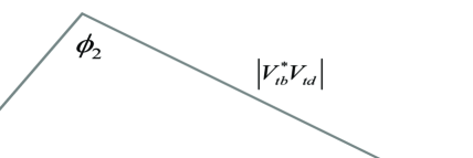
   Figure 2: The CKM Unitarity Triangle

   The sides of this triangle having naturally large angles, see Fig.(2), are given by $\lambda\cdot V(cb)$, $V(ub)$ and $V^{*}(td)$; these are all quantities that control important aspects of $B$ decays, namely CKM favoured and disfavoured $B_{u,d}$ decays and $B_{d}-\bar{B}_{d}$ oscillations. The $B_{d}$ triangle of Eq.(141) is usually referred to as ‘the’ CKM unitarity triangle.

Let the reader be reminded that all six triangles, despite their very different shapes, have the same area, see Eq.(34), reflecting the single CKM phase for three families.

Some comments on notation might not be completely useless. The BABAR collaboration and its followers refer to the three angles of the CKM unitarity triangle as $\alpha$, $\beta$ and $\gamma$; the BELLE collaboration instead has adopted the notation $\phi_{1}$, $\phi_{2}$ and $\phi_{3}$. While it poses no problem to be conversant in both languages, the latter has not only historical priority on its side [20], but is also more rational. For the angles $\phi_{i}$ in the ‘$bd$’ triangle of Eq.(141) are always opposite the side defined by $V^{*}(id)V(ib)$. Furthermore this classification scheme can readily be generalized to all six unitarity triangles; those triangles can be labeled by $kl$ with $k\neq l=d,s,b$ or $k\neq l=u,c,t$, see Eqs.(137) – (142). Its 18 angles can then be unambiguously denoted by $\phi_{i}^{kl}$: it is the angle in triangle $kl$ opposite the side $V^{*}(ik)V(il)$ or $V^{*}(ki)V(li)$, respectively. Therefore I view the notation $\phi_{i}^{(kl)}$ as the only truly Cartesian one.

The discovery of $B_{d}-\bar{B}_{d}$ oscillations defined the ‘CKM Paradigm of Large CP Violation in $B$ Decays’ that had been anticipated in 1980:

• A host of nonleptonic $B$ channels has to exhibit sizable CP asymmetries.

• For $B_{d}$ decays to flavour-nonspecific final states (like CP eigenstates) the CP asymmetries depend on the time of decay in a very characteristic manner; their size should typically be measured in units of 10% rather than 0.1%.

• There is no plausible deniability for the CKM description, if such asymmetries are not found.

• For $m_{t}\geq 150$ GeV the SM prediction for $\epsilon_{K}$ is dominated by the top quark contribution like $\Delta M_{B_{d}}$. It thus drops out from their ratio, and sin$2\phi_{1}$ can be predicted within the SM irrespective of the (superheavy) top quark mass. In the early 1990’s, i.e., before the direct discovery of top quarks, it was predicted [21]

  $$\frac{\epsilon_{K}}{\Delta M_{B_{d}}}\propto{\rm sin}2\phi_{1}\sim 0.6-0.7$$ (144)

  with values for $B_{B}f_{B}^{2}$ inserted as now estimated by LQCD.

• The CP asymmetry in the Cabibbo favoured channels $B_{s}\to\psi\phi/\psi\eta$ is Cabibbo suppressed, i.e. below 4%, for reasons very specific to CKM theory, as pointed out already in 1980 [12].

In 1974 finally top quarks were observed directly with a mass fully consistent with the indirect estimates given above; the most recent analyses from CDF & D0 list

$$m_{t}=172.7\pm 2.9\;{\rm GeV}$$ (145)

Data in 1998

CP violation had been observed only in the decays of neutral kaons, and all its manifestations – $K_{L}\to\pi^{+}\pi^{-}$, $\pi^{0}\pi^{0}$, $K^{0}\to\pi^{+}\pi^{-}$ vs. $\bar{K}^{0}\to\pi^{+}\pi^{-}$, $K_{L}\to l^{+}\nu\pi^{-}$ vs. $K_{L}\to l^{-}\bar{\nu}\pi^{+}$ – could be described for 35 years with a single real number, namely $|\eta_{+-}|$ or $\Phi(\Delta S=2)={\rm arg}(M_{12}/\Gamma_{12})$.

There was intriguing, though not conclusive evidence for direct CP violation:

$$\frac{\epsilon^{\prime}}{\epsilon_{K}}=\left\{\begin{array}[]{ll}(2.30\pm 0.65)\cdot 10^{-3}&{\rm NA31}\\ (0.74\pm 0.59)\cdot 10^{-3}&{\rm E731}\end{array}\right.$$ (146)

These measurements were made in the 1980’s and had been launched by theory guestimates suggesting values for $\epsilon^{\prime}$ that would be within the reach of these experiments. Theory, however, had ‘moved on’ favouring values $\leq 10^{-3}$ – or so it was claimed.

0.1.8 Completion of a Heroic Era

Direct CP violation has been unequivocally established in 1999. The present world average dominated by the data from NA48 and KTeV reads as follows [22]:

$$\langle\epsilon^{\prime}/\epsilon_{K}\rangle=(1.63\pm 0.22)\cdot 10^{-3}$$ (147)

Quoting the result in this way does not do justice to the experimental achievement, since $\epsilon_{K}$ is a very small number itself. The sensitivity achieved becomes more obvious when quoted in terms of actual widths [22]:

$$\frac{\Gamma(K^{0}\to\pi^{+}\pi^{-})-\Gamma(\bar{K}^{0}\to\pi^{+}\pi^{-})}{\Gamma(K^{0}\to\pi^{+}\pi^{-})+\Gamma(\bar{K}^{0}\to\pi^{+}\pi^{-})}=(5.04\pm 0.82)\cdot 10^{-6}\;!$$ (148)

This represents a discovery of the very first rank . Its significance does not depend on whether the SM can reproduce it or not – which is the most concise confirmation of how important it is. The HEP community can take pride in this achievement; the tale behind it is a most fascinating one about imagination and perseverance. The two groups and their predecessors deserve our respect; they have certainly earned my admiration.

The experimental findings are consistent with CKM theory on the qualitative level, since the latter does not represent a superweak scenario even for strange decays due to the existence of Penguin operators. It is not inconsistent with it even quantitatively. One should keep in mind that within the SM $\epsilon^{\prime}/\epsilon_{K}$ has to be considerably suppressed. $\epsilon^{\prime}$ requires interference between $\Delta I=1/2\,\&\,3/2$ amplitudes and is thus reduced by the ‘$\Delta I=1/2$ rule’: $|T(\Delta I=3/2)/T(\Delta I=1/2)|\sim 1/20$. Furthermore $\epsilon^{\prime}$ is generated by loop diagrams – as is $\epsilon_{K}$; yet the top quark mass enhances $\epsilon_{K}$ powerlike – $|\epsilon_{K}|\propto m_{t}^{2}/M_{W}^{2}$ – whereas $\epsilon^{\prime}$ only logarithmically. When there is only one weak phase – as is the case for CKM theory – one has $|\epsilon^{\prime}/\epsilon_{K}|\propto{\rm log}m_{t}^{2}/m_{t}^{2}$, i.e. greatly reduced again for superheavy top quarks (revisit Homework # 4).

CKM theory can go beyond such semiquantitative statements, but one should not expect a precise prediction from it in the near future. For the problem of uncertainties in the evaluation of hadronic matrix elements is compounded by the fact that the two main contributions to $\epsilon^{\prime}$ are similar in magnitude, yet opposite in sign [23].

CKM Theory at the End of the 2nd Millenium

It is indeed true that large fractions of the observed values for $\Delta M_{K}$, $\epsilon_{K}$ and $\Delta M_{B}$ and even most of $\epsilon^{\prime}$ could be due to New Physics given the limitations in our theoretical control over hadronic matrix elements. Equivalently constraints from these and other data translate into ‘broad’ bands in plots of the unitarity triangle, see Fig.3.

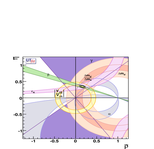
Figure 3: The CKM Unitarity Triangle fit.

The problem with this statement is that it is not even wrong – it misses the real point. Let me illustrate it by a local example first. If you plot the whereabouts of the students at this school on a local map, you would find a seemingly broad band stretching from Aronsborg to Stockholm and Uppsala; however when you look at the ‘big’ picture – say a map of Europe – you realize these students are very closely bunched together in one tiny spot on the map. This cannot be by accident, there has to be a good reason for it, which, I hope, is obvious in this specific case. Likewise for the problem at hand: Observables like $\Gamma(B\to l\nu X_{c,u})$, $\Gamma(K\to l\nu\pi)$, $\Delta M_{K}$, $\Delta M_{B}$, $\epsilon_{K}$ and sin$2\phi_{1}$ etc. represent very different dynamical regimes that proceed on time scales hat span several orders of magnitude. The very fact that CKM theory can accommodate such diverse observables always within a factor two or better and relate them in such a manner that its parameters can be plotted as meaningful constraints on a triangle is highly nontrivial and – in my view – must reflect some underlying, yet unknown dynamical layer. Furthermore the CKM parameters exhibit an unusual hierarchical pattern – $|V(ud)|\sim|V(cs)|\sim|V(tb)|\sim 1$, $|V(us)|\simeq|V(cd)|\simeq\lambda$, $|V(cb)|\sim|V(ts)|\sim{\cal O}(\lambda^{2})$, $|V(ub)|\sim|V(td)|\sim{\cal O}(\lambda^{3})$ – as do the quark masses culminating in $m_{t}\simeq 175$ GeV. Picking such values for these parameters would have been seen as frivolous at best – had they not been forced upon us by (independent) data. Thus I view it already as a big success for CKM theory that the experimental constraints on its parameters can be represented through triangle plots in a meaningful way.

Interlude: Singing the Praise of Hadronization

Hadronization and nonperturbative dynamics in general are usually viewed as unwelcome complication, if not outright nuisances. A case in point was already mentioned: while I view the CKM predictions for $\Delta M_{K}$, $\Delta M_{B}$, $\epsilon_{K}$ to be in remarkable agreement with the data, significant contributions from New Physics could be hiding there behind the theoretical uncertainties due to lack of computational control over hadronization. Yet without hadronization bound states of quarks and antiquarks will not form; without the existence of kaons $K^{0}-\bar{K}^{0}$ oscillations obviously cannot occur. It is hadronization that provides the ‘cooling’ of the (anti)quark degrees of freedom, which allows subtle quantum mechanical effects to add up coherently over macroscopic distances. Otherwise one would not have access to a super-tiny energy difference Im${\cal M}_{12}\sim 10^{-8}$ eV, which is very sensitive to different layers of dynamics, and indirect CP violation could not manifest itself. The same would hold for $B$ mesons and $B^{0}-\bar{B}^{0}$ oscillations.

To express it in a more down to earth way:

• Hadronization leads to the formation of kaons and pions with masses exceeding greatly (current) quark masses. It is the hadronic phase space that suppresses the CP conserving rate for $K_{L}\to 3\pi$ by a factor $\sim 500$, since the $K_{L}$ barely resides above the three pion threshold.

• It awards ‘patience’; i.e. one can ‘wait’ for a pure $K_{L}$ beam to emerge after starting out with a beam consisting of $K^{0}$ and $\bar{K}^{0}$.

• It enables CP violation to emerge in the existence of a reaction, namely $K_{L}\to 2\pi$ rather than an asymmetry; this greatly facilitates its observation.

For these reasons alone we should praise hadronization as the hero in the tale of CP violation rather than the villain it is all too often portrayed.

End of Interlude

Looking at the present CKM triangle fit shown in Fig. 3 one realizes another triumph of CKM theory appears imminent: if one removed at present the constraints from $\epsilon_{K}$ and sin$2\phi_{1}$, i.e. CP constraints, then a ‘flat’ CKM ‘triangle’ is barely compatible with the constraints on $|V(td)|$ from $\Delta M(B_{d})$ and on $|V(ub)/V(cb)|$ from semileptonic $B$ decays – processes not sensitive to CP violation per se. However a measurement of $\Delta M(B_{s})$ through resolving $B_{s}-\bar{B}_{s}$ oscillations in the near future would definitely require this triangle to be nontrivial: ‘CP insensitive observables would imply CP violation’!

The first unequivocal manifestation of a Penguin contribution surfaced in radiative $B$ decays, first the exclusive channel $B\to\gamma K^{*}$ and subsequently the inclusive one $B\to\gamma X_{s}$. These transitions represent flavour changing neutral currents and as such represent a one-loop, i.e. quantum process.

By the end of the second millenium a rich and diverse body of data on flavour dynamics had been accumulated, and CKM theory provided a surprisingly successful description of it. This prompted some daring spirits to perform detailed fits of the CKM triangle to infer a rather accurate prediction for the CP asymmetry in $B_{d}\to\psi K_{S}$ [24]:

$${\rm sin}2\phi_{1}=0.72\pm 0.07$$ (149)

0.1.9 Summary of Lecture I

The status of flavour dynamics in general and of CKM theory in particular in just before the turn of the millenium can be summarized as follows:

• "Never underestimate Nature’s ability to come up with an unexpected trick." Physicists had thought to have seen it all after the shock of parity violation in 1957 – and then the ‘earthquake’ of CP violation struck in 1964.

• "CKM theory – all it does, it works." We have only an ‘engineering’ solution for the generation of masses (the Higgs mechanism), yet no deeper understanding in particular of fermion masses and family replication. Yet CKM theory, which is based on a set of mass related parameters (fermion masses, CKM parameters) that any sober person would view as frivolous – were they not forced upon us by data – describes successfully a vast and very diverse array of transitions characterized by dynamical scales that a priori span several orders of magnitude.

• While no accurate CKM prediction for $\epsilon^{\prime}/\epsilon_{K}$ is available now (and presumably for some time to come), it is highly nontrivial that the predictions match to data to better than an order of magnitude. It provides some understanding why direct CP violation is so feeble in kaon decays: it is greatly reduced by the $\Delta I=1/2$ rule – i.e. $T(S=1;\Delta I=3/2)/T(S=1;\Delta I=1/2)\simeq 1/20$ – and the unexpectedly large top quark mass.

• The SM has to produce a host of truly large CP asymmetries in $B$ decays – there is no plausible deniability. This is far from trivial: based on a tiny CP impurity in the $K^{0}-\bar{K}^{0}$ system one predicts an almost maximal CP asymmetry in $B_{d}$ decays:

  $${\rm few}\times 0.001\;{\rm{\bf CP}~{}asymm.\;in\;}K^{0}-\bar{K}^{0}\hskip 28.45274pt\Longrightarrow\hskip 28.45274pt{\rm few}\times 0.1\;{\rm{\bf CP}~{}asymm.\;in\;}B_{d}-\bar{B}_{d}\;;$$ (150)

  i.e., an effect two orders of magnitude larger.

• While it is quite possible, or even likely, that New Physics will affect CP asymmetries in $B$ decays, we cannot expect it to create a numerically massive impact except for some special cases.

0.2 Lecture II: "Flavour Dynamics 2000 - 2006" – The ‘Expected’ Triumph of a Peculiar Theory

As explained in the previous lecture, within CKM theory one is unequivocally lead to a paradigm of large CP violation in $B$ decays. This realization became so widely accepted that two $B$ factories employing $e^{+}e^{-}\to\Upsilon(4S)\to B\bar{B}$ were constructed – one at KEK in Japan and one in Stanford in the US – together with specialized detectors, around which two collaborations gathered, the BELLE and BABAR collaborations, respectively.

0.2.1 Establishing the CKM Ansatz as a Theory – CP Violation in $B$ Decays

The three angles $\phi_{1,2,3}$ in the CKM unitarity triangle (see Fig.2 for notation) can be determined through CP asymmetries in $B_{d}(t)\to\psi K_{S},\pi^{+}\pi^{-}$ and $B_{d}\to K^{+}\pi^{-}$ – in principle. In practice the angle $\phi_{3}$ can be extracted from $B^{\pm}\to D^{\rm neut}K^{\pm}$ with better theoretical control, and $B\to 3\pi,\;4\pi$ offer various experimental advantages over $B\to 2\pi$. These issues will be addressed in five acts plus two interludes.

Act I: $B_{d}(t)\to\psi K_{S}$ and $\phi_{1}$ (a.k.a. $\beta$)

The first published result on the CP asymmetry in $B_{d}\to\psi K_{S}$ was actually obtained by the OPAL collaboration at LEP I [25]:

$${\rm sin}2\phi_{1}=3.2^{+1.8}_{-2.0}\pm 0.5\;,$$ (151)

where the ‘unphysical’ value of sin$2\phi_{1}$ is made possible, since a large background subtraction has to be performed. The first value inside the physical range was obtained by CDF [26] :

$${\rm sin}2\phi_{1}=0.79\pm 0.44$$ (152)

In 2000 the two $B$ factory collaborations BABAR and BELLE presented their first measurements [17]:

$${\rm sin}2\phi_{1}=\left\{\begin{array}[]{l}0.12\pm 0.37\pm 0.09\;\;{\rm BABAR\;^{\prime}00}\\ 0.45\pm 0.44\pm 0.09\;\;{\rm BELLE\;^{\prime}00}\end{array}\right.$$ (153)

Already one year later these inconclusive numbers turned into conclusive ones, and the first CP violation outside the $K^{0}-\bar{K}^{0}$ complex was established:

$${\rm sin}2\phi_{1}=\left\{\begin{array}[]{l}0.59\pm 0.14\pm 0.05\;\;{\rm BABAR\;^{\prime}01}\\ 0.99\pm 0.14\pm 0.06\;\;{\rm BELLE\;^{\prime}01}\end{array}\right.$$ (154)

By 2003 the numbers from the two experiments had well converged

$${\rm sin}2\phi_{1}=\left\{\begin{array}[]{l}0.741\pm 0.067\pm 0.03\;\;{\rm BABAR\;^{\prime}03}\\ 0.733\pm 0.057\pm 0.028\;\;{\rm BELLE\;^{\prime}03}\end{array}\right.$$ (155)

allowing one to state just the world averages, which is actually a BABAR/BELLE average [17]:

$${\rm sin}2\phi_{1}=\left\{\begin{array}[]{l}0.726\pm 0.037\;\;{\rm WA\;^{\prime}04}\\ 0.685\pm 0.032\;\;{\rm WA\;^{\prime}05}\\ 0.675\pm 0.026\;\;{\rm WA\;^{\prime}06}\end{array}\right.$$ (156)

The CP asymmetry in $B_{d}\to\psi K_{S}$ is there, is huge and as expected even quantitatively. For CKM fits based on constraints from $|V(ub)/V(cb)|$, $B^{0}-\bar{B}^{0}$ oscillations and – as the only CP sensitive observable – $\epsilon_{K}$ yield [27]

$${\rm sin}2\phi_{1}|_{\rm CKM}=0.755\pm 0.039\;.$$ (157)

The CKM prediction has stayed within the $\sim 0.72-0.75$ interval for the last several years. Through 2005 it has been in impressive agreement with the data. In 2006 a hint of a deviation has emerged. It is not more than that, since it is not (yet) statistically significant and furthermore depends very much on the value extracted for $|V(ub)/V(cb)|$ and its uncertainty. The latter might very well be underestimated, as discussed later. This is illustrated by Fig.3 showing these constraints. This figure actually obscures another impressive triumph of CKM theory: the CP insensitive observables $|V(ub)/V(cb)|$ and $\Delta M(B_{d})/\Delta M(B_{s})$ – i.e. observables that do not require CP violation for acquiring a non-zero value – imply

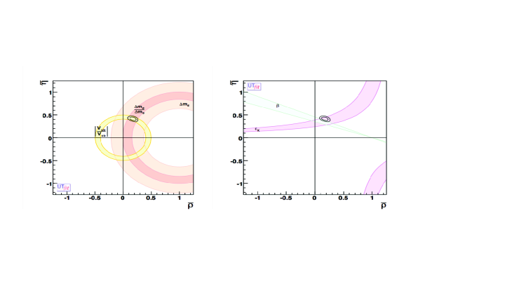
Figure 4: CKM unitarity triangle from $|V(ub)/V(cb)|$ and $\Delta M(B_{d})/\Delta M(B_{s})$ on the left and compared to constraints from $\epsilon_{K}$ and sin2$\phi_{1}/\beta$ on the right (courtesy of M. Pierini)

• a non-flat CKM triangle and thus CP violation, see the left of Fig. 4

• that is fully consistent with the observed CP sensitive observables $\epsilon_{K}$ and sin$2\phi_{1}$, see the right of Fig. 4.

CP violation in $K$ and $B$ decays – exactly the same, only different

There are several similarities between $K^{0}-\bar{K}^{0}$ and $B_{d}-\bar{B}_{d}$ oscillations even on the quantitative level. Their values for $x=\Delta M/\Gamma$ and thus for $\chi$ are very similar. It is even more intriguing that also their pattern of CP asymmetries in $K^{0}(t)/\bar{K}^{0}(t)\to\pi^{+}\pi^{-}$ and $B_{d}(t)/\bar{B}_{d}(t)\to\psi K_{S}$ is very similar. Consider the two lower plots in Fig.5, which show the asymmetry directly as a function of $\Delta t$: it looks intriguingly similar qualitatively and even quantitatively. The lower left plot shows that the difference between $K^{0}\to\pi^{+}\pi^{-}$ and $\bar{K}^{0}\to\pi^{+}\pi^{-}$ is actually measured in units of 10 % for $\Delta t\sim(8-16)\tau_{K_{S}}$, which is the $K_{S}-K_{L}$ interference region.

Clearly one can find domains in $K\to\pi^{+}\pi^{-}$ that exhibit a truly large CP asymmetry. Nevertheless it is an empirical fact that CP violation in $B$ decays is much larger than in $K$ decays. For the mass eigenstates of neutral kaons are very well approximated by CP eigenstates, as can be read off from the upper left plot: it shows that the vast majority of $K\to\pi^{+}\pi^{-}$ events follow a single exponential decay law that coincides for $K^{0}$ and $\bar{K}^{0}$ transitions. This is in marked contrast to the $B_{d}\to\psi K_{S}$ and $\bar{B}_{d}\to\psi K_{S}$ transitions, which in no domain are well approximated by a single exponential law and do not coincide at all, except for $\Delta t=0$, as it has to be, see Sect.0.2.1.

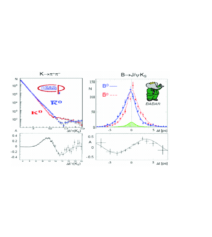
Figure 5: The observed decay time distributions for $K^{0}$ vs. $\bar{K}^{0}$ from CPLEAR on the left and for $B_{d}$ vs.$\bar{B}_{d}$ from BABAR on the right.

Interlude: "Praise the Gods Twice for EPR Correlations"

The BABAR and BELLE analyses are based on a glorious application of quantum mechanics and in particular EPR correlations[28]. The CP asymmetry in $B_{d}\to\psi K_{S}$ had been predicted to exhibit a peculiar dependence on the time of decay, since it involves $B_{d}-\bar{B}_{d}$ oscillations in an essential way:

$${\rm rate}(B_{d}(t)[\bar{B}_{d}(t)]\to\psi K_{S})\propto e^{-t/\tau_{B}}(1-[+]A{\rm sin}\Delta m_{B}t)\;,$$ (158)

At first it would seem that an asymmetry of the form given in Eq.(158) could not be measured for practical reasons. For in the reaction

$$e^{+}e^{-}\to\Upsilon(4S)\to B_{d}\bar{B}_{d}$$ (159)

the point where the $B$ meson pair is produced is ill determined due to the finite size of the electron and positron beam spots: the latter amounts to about 1 mm in the longitudinal direction, while a $B$ meson typically travels only about a quarter of that distance before it decays. It would then seem that the length of the flight path of the $B$ mesons is poorly known and that averaging over this ignorance would greatly dilute or even eliminate the signal.

It is here where the existence of a EPR correlation comes to the rescue. While the two $B$ mesons in the reaction of Eq.(159) oscillate back and forth between a $B_{d}$ and $\bar{B}_{d}$, they change their flavour identity in a completely correlated way. For the $B\bar{B}$ pair forms a C odd state; Bose statistics then tells us that there cannot be two identical flavour hadrons in the final state:

$$e^{+}e^{-}\to\Upsilon(4S)\to B_{d}\bar{B}_{d}\not\to B_{d}B_{d},\;\bar{B}_{d}\bar{B}_{d}$$ (160)

Once one of the $B$ mesons decays through a flavour specific mode, say $B_{d}\to l^{+}\nu X$ [$\bar{B}_{d}\to l^{-}\bar{\nu}X$], then we know unequivocally that the other $B$ meson was a $\bar{B}_{d}$ [$B_{d}$] at that time. The time evolution of $\bar{B}_{d}(t)[B_{d}(t)]\to\psi K_{S}$ as described by Eq.(158) starts at that time as well; i.e., the relevant time parameter is the interval between the two times of decay, not those times themselves. That time interval is related to – and thus can be inferred from – the distance between the two decay vertices, which is well defined and can be measured.

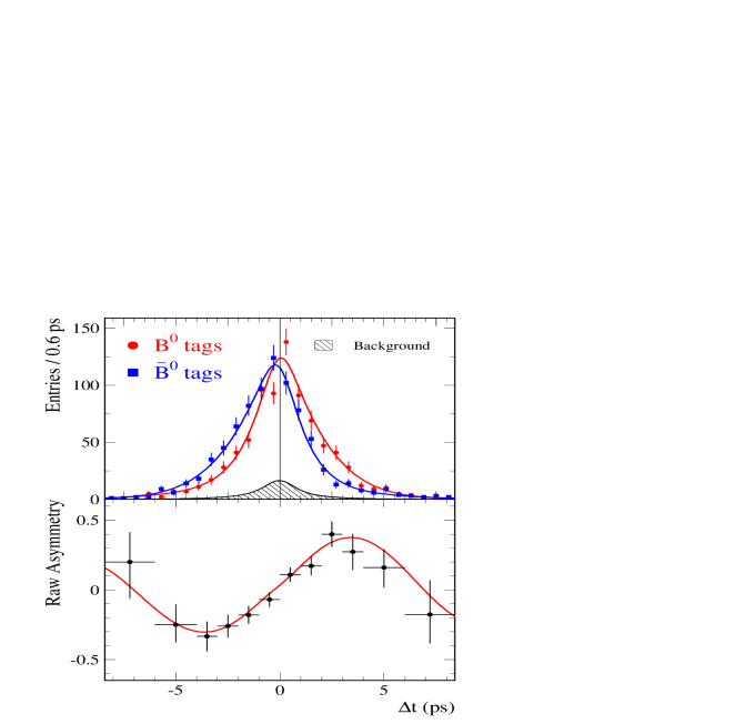
Figure 6: The observed decay time distributions for $B^{0}$ (red) and $\bar{B}^{0}$ (blue) decays.

The great practical value of the EPR correlation is instrumental for another consideration as well, namely how to see directly from the data that CP violation is matched by T violation. Fig.6 shows two distributions, one for the interval $\Delta t$ between the times of decays $B_{d}\to l^{+}X$ and $\bar{B}_{d}\to\psi K_{S}$ and the other one for the CP conjugate process $\bar{B}_{d}\to l^{-}X$ and $B_{d}\to\psi K_{S}$. They are clearly different proving that CP is broken. Yet they show more: the shape of the two distributions is actually the same (within experimental uncertainties) the only difference being that the average of $\Delta t$ is positive for $(l^{-}X)_{\bar{B}}(\psi K_{S})$ and negative for $(l^{+}X)_{B}(\psi K_{S})$ events. I.e., there is a (slight) preference for $B_{d}\to\psi K_{S}$ [$\bar{B}_{d}\to\psi K_{S}$] to occur after [before] and thus more [less] slowly (rather than just more rarely) than $\bar{B}\to l^{-}X$ [$B\to l^{+}X$]. Invoking CPT invariance merely for semileptonic $B$ decays – yet not for nonleptonic transitions – synchronizes the starting point of the $B$ and $\bar{B}$ decay ‘clocks’, and the EPR correlation keeps them synchronized. We thus see that CP and T violation are ‘just’ different sides of the same coin. As explained above, EPR correlations are essential for this argument!

The reader can be forgiven for feeling that this argument is of academic interest only, since CPT invariance of all processes is based on very general arguments. Yet the main point to be noted is that EPR correlations, which represent some of quantum mechanics’ most puzzling features, serve as an essential precision tool, which is routinely used in these measurements. I feel it is thus inappropriate to refer to EPR correlations as a paradox.

Act II: $B_{d}(t)\to pions$ and $\phi_{2}$ (a.k.a. $\alpha$)

$B\to 2\pi$

The situation is theoretically more complex than for $B_{d}(t)\to\psi K_{S}$ due to two reasons:

• While both final states $\pi\pi$ and $\psi K_{S}$ are CP eigenstates, the former unlike the latter is not reached through an isoscalar transition. The two pions can form an $I=0$ or $I=2$ configuration (similar to $K\to 2\pi$), which in general will be affected differently by the strong interactions.

• For all practical purposes $B_{d}\to\psi K_{S}$ is described by two tree diagrams representing the two effective operators $(\bar{c}_{L}\gamma_{\mu}b_{L})(\bar{s}_{L}\gamma^{\mu}c_{L})$ and $(\bar{c}_{L}\gamma_{\mu}\lambda_{i}b_{L})(\bar{s}_{L}\gamma^{\mu}\lambda_{i}c_{L})$ with the $\lambda_{i}$ representing the $SU(3)_{C}$ matrices. Yet for $B\to\pi\pi$ we have effective operators $(\bar{d}_{L}\gamma_{\mu}\lambda_{i}b_{L})(\bar{q}\gamma^{\mu}\lambda_{i}q)$ generated by the Cabibbo suppressed Penguin loop diagrams in addition to the two tree operators $(\bar{u}_{L}\gamma_{\mu}b_{L})(\bar{d}_{L}\gamma^{\mu}u_{L})$ and $(\bar{u}_{L}\gamma_{\mu}\lambda_{i}b_{L})(\bar{d}_{L}\gamma^{\mu}\lambda_{i}u_{L})$.

This greater complexity manifests itself already in the phenomenological description of the time dependent CP asymmetry:

$$\frac{R_{+}(\Delta t)-R_{-}(\Delta t)}{R_{+}(\Delta t)+R_{-}(\Delta t)}=S{\rm sin}(\Delta M_{d}\Delta t)-C{\rm cos}(\Delta M_{d}\Delta t)\;,\;S^{2}+C^{2}\leq 1$$ (161)

where $R_{+[-]}(\Delta t)$ denotes the rate for $B^{tag}(t)\bar{B}_{d}(t+\Delta)[\bar{B}^{tag}(t)B_{d}(t+\Delta)]$ and

$$S=\frac{2{\rm Im}\frac{q}{p}\bar{\rho}_{\pi^{+}\pi^{-}}}{1+\left|\frac{q}{p}\bar{\rho}_{\pi^{+}\pi^{-}}\right|^{2}}\;,\;\;C=\frac{1-\left|\frac{q}{p}\bar{\rho}_{\pi^{+}\pi^{-}}\right|^{2}}{1+\left|\frac{q}{p}\bar{\rho}_{\pi^{+}\pi^{-}}\right|^{2}}$$ (162)

As before, due to the EPR correlation between the two neutral $B$ mesons, it is the relative time interval $\Delta t$ between the two $B$ decays that matters, not their lifetime. The new feature is that one has also a cosine dependence on $\Delta t$.

BABAR and BELLE find

$$S = \left\{\begin{array}[]{l}-0.53\pm 0.14\pm 0.02\;\;{\rm BABAR\;^{\prime}06}\\ -0.61\pm 0.10\pm 0.04\;\;{\rm BELLE\;^{\prime}06}\\ -0.59\pm 0.09\hskip 39.83368pt{\rm HFAG}\end{array}\right.$$ (166)

$$C = \left\{\begin{array}[]{l}-0.16\pm 0.11\pm 0.03\;\;{\rm BABAR\;^{\prime}06}\\ -0.55\pm 0.08\pm 0.05\;\;{\rm BELLE\;^{\prime}06}\\ -0.39\pm 0.07\hskip 39.83368pt{\rm HFAG}\end{array}\right.$$ (170)

While BABAR and BELLE agree nicely on $S$ making the HFAG average straightforward, their findings on $C$ indicate different messages making the HFAG average more iffy.

$S\neq 0$ has been established and thus CP violation also in this channel. While BELLE finds $C\neq 0$ as well, BABAR’s number is still consistent with $C=0$. $C\neq 0$ obviously represents direct CP violation. Yet it is often overlooked that also $S$ can reveal such CP violation. For if one studies $B_{d}$ decays into two CP eigenstates $f_{a}$ and $f_{b}$ and finds

$$S(f_{a})\neq\eta(f_{a})\eta(f_{b})S(f_{b})$$ (171)

with $\eta_{i}$ denoting the CP parities of $f_{i}$, then one has established direct CP violation. For the case under study that means even if $C(\pi\pi)=0$, yet $S(\pi^{+}\pi^{-})\neq-S(\psi K_{S})$, one has observed unequivocally direct CP violation. One should note that such direct CP violation might not necessarily induce $C\neq 0$. For the latter requires, as explained below in Sect. 0.2.1 (see Eq.(179)), that two different amplitudes contribute coherently to $B_{d}\to f_{b}$ with non-zero relative weak as well as strong phases. $S(f_{a})\neq\eta(f_{a})\eta(f_{b})S(f_{b})$ on the other hand only requires that the two overall amplitudes for $B_{d}\to f_{a}$ and $B_{d}\to f_{b}$ possess a relative phase. This can be illustrated with a familiar example from CKM dynamics: If there were no Penguin operators for $B_{d}\to\pi^{+}\pi^{-}$ (or it could be ignored quantitatively), one would have $C(\pi^{+}\pi^{-})=0$, yet at the same time $S(\psi K_{S})={\rm sin}(2\phi_{1})$ together with $S(\pi^{+}\pi^{-})={\rm sin}(2\phi_{2})\neq-{\rm sin}(2\phi_{1})$. I.e., without direct CP violation one would have to find $C=0$ and $S=-{\rm sin}2\phi_{1}$ [29]. Yet since the measured value of $S$ is within one sigma of - sin$2\phi_{1}$ this distinction is mainly of academic interest at the moment.

Once the categorical issue of whether there is direct CP violation has been settled, one can take up the challenge of extracting a value for $\phi_{2}$ from the data . This can be done in a model independent way by analyzing $B_{d}(t)\to\pi^{+}\pi^{-}$, $\pi^{0}\pi^{0}$ and $B^{\pm}\to\pi^{\pm}\pi^{0}$ transitions and performing an isospin decomposition. For the Penguin contribution cannot affect $B_{d}(t)\to[\pi\pi]_{I=2}$ modes. Unfortunately there is a serious experimental bottle neck, namely to study $B_{d}(t)\to\pi^{0}\pi^{0}$ with sufficient accuracy. Therefore alternative decays have been suggested, in particular $B\to\rho\pi$ and $\rho\rho$.

$B\to 3\pi/4\pi$

The final states in $B\to 3\pi$ and $4\pi$ are largely of the $\rho\pi$ and $\rho\rho$ form, respectively. For those one can also undertake an isospin decomposition to disentangle the Penguin contribution. These channels are less challenging experimentally than $B_{d,u}\to 2\pi$, yet they pose some complex theoretical problems.

For going from the experimental starting point $B\to 3\pi$ to $B\to\pi\rho$ configurations is quite nontrivial. There are other contributions to the three-pion final state like $\sigma\pi$, and cutting on the dipion mass provides a rather imperfect filter due to the large $\rho$ width. It hardly matters in this context whether the $\sigma$ is a bona fide resonance or some other dynamical enhancement. This actually leads to a further complication, namely that the $\sigma$ structure cannot be described adequately by a Breit-Wigner shape. As analyzed first in [30] and then in more detail in [31] ignoring such complications can induce a significant systematic uncertainty in the extracted value of $\phi_{2}$.

The modes $B_{d,u}\to\rho\rho$ contain even more theoretical complexities, since they have to be extracted from $B\to 4\pi$ final states, where one has to allow for $\sigma\rho$, $2\sigma$, $\rho 2\pi$ etc. in addition to $2\rho$.

My point here is one of caution rather than of agnosticism. The concerns sketched above might well be more academic than practical with the present statistics. My main conclusions are the following: (i) I remain unpersuaded that averaging over the values for $\phi_{2}$ obtained so far from the three methods listed above provides a reliable value, since I do not think that the systematic uncertainties have sufficiently been analyzed. (ii) It will be mandatory to study those in a comprehensive way, before we can make full use of the even larger data sets that will become available in the next few years. As I have emphasized repeatedly, our aim has to be to reduce the uncertainty down to at least the 5% level in a way that can be defended. (iii) In the end we will need

• to perform time dependent Dalitz plot analyses (and their generalizations) and

• involve the expertise that already exists or can obtained concerning low-energy hadronization processes like final state interactions among low energy pions and kaons; valuable information can be gained on those issues from $D_{(s)}\to\pi$’s, kaons etc. as well as $D_{(s)}\to l\nu K\pi/\pi\pi/KK$, in particular when analyzed with state-of-the-art tools of chiral dynamics.

Act III, $1^{st}$ Version: $B_{d}\to K^{+}\pi^{-}$

It was pointed out in a seminal paper [32] that (rare) transitions like $\bar{B}_{d}\to K^{-}+\pi$’s have the ingredients for sizable direct CP asymmetries:

• Two different amplitudes can contribute coherently, namely the highly CKM suppressed tree diagram with $b\to u\bar{u}s$ and the Penguin diagram with $b\to s\bar{q}q$.

• The tree diagram contains a large weak phase from $V(ub)$.

• The Penguin diagram with an internal charm quark loop exhibits an imaginary part, which can be viewed – at least qualitatively – as a strong phase generated by the production and subsequent annihilation of a $c\bar{c}$ pair (the diagram with an internal $u$ quark loop acts merely as a subtraction point allowing a proper definition of the operator).

• While the Penguin diagram with an internal top quark loop is actually not essential, the corresponding effective operator can be calculated quite reliably, since integrating out first the top quarks and then the $W$ boson leads to a truly local operator. Determining its matrix elements is however another matter.

To translate these features into accurate numbers represents a formidable task, we have not mastered yet. In Ref. [33] an early and detailed effort was made to treat $\bar{B}_{d}\to K^{-}\pi^{+}$ theoretically with the following results:

$${\rm BR}(\bar{B}_{d}\to K^{-}\pi^{+})\sim 10^{-5}\;,\;\;A_{{\bf CP}}\sim-0.10$$ (172)

Those numbers turn out to be rather prescient, since they are in gratifying agreement with the data

$${\rm BR}(\bar{B}_{d}\to K^{-}\pi^{+})=(1.85\pm 0.11)\cdot 10^{-5}$$

$$A_{{\bf CP}}=\left\{\begin{array}[]{l}-0.133\pm 0.030\pm 0.009\;\;\;{\rm BABAR}\\ -0.113\pm 0.021\;\;\;{\rm BELLE}\end{array}\right.$$ (173)

Cynics might point out that the authors in [33] did not give a specific estimate of the theoretical uncertainties in Eq.(172). More recent authors have been more ambitious – with somewhat mixed success. I list the predictions inferred from pQCD [34] and QCD Factorization [35] and the data for the three modes $\bar{B}_{d}\to K^{-}\pi^{+}$ and $B^{-}\to K^{-}\pi^{0},\,\bar{K}^{0}\pi^{-}$:

$$A_{{\bf CP}}(B_{d}\to K^{-}\pi^{+})=\left\{\begin{array}[]{l}-0.133\pm 0.030\pm 0.009\;\;\;{\rm BABAR}\\ -0.113\pm 0.021\;\;\;{\rm BELLE}\\ -0.09^{+0.05+0.04}_{-0.08-0.06}\;\;\;{\rm pQCD}\\ +0.05\pm 0.09\;\;\;{\rm QCD\;Fact.}\end{array}\right.$$ (174)

$$A_{{\bf CP}}(B^{-}\to K^{-}\pi^{0})=\left\{\begin{array}[]{l}+0.06\pm 0.06\pm 0.01\;\;\;{\rm BABAR}\\ +0.04\pm 0.04\pm 0.02\;\;\;{\rm BELLE}\\ -0.01^{+0.03+0.03}_{-0.05-0.05}\;\;\;{\rm pQCD}\\ +0.07\pm 0.09\;\;\;{\rm QCD\;Fact.}\end{array}\right.$$ (175)

$$A_{{\bf CP}}(B^{-}\to\bar{K}^{0}\pi^{-})=\left\{\begin{array}[]{l}-0.09\pm 0.05\pm 0.01\;\;\;{\rm BABAR}\\ +0.05\pm 0.05\pm 0.01\;\;\;{\rm BELLE}\\ +0.00\;\;\;{\rm pQCD}\\ +0.01\pm 0.01\;\;\;{\rm QCD\;Fact.}\end{array}\right.$$ (176)

As explained next the size of these asymmetries depends very much on hadronization effecs, namely hadronic matrix elements and strong phase shifts. While the observed asymmetry in $B_{d}\to K\pi$ with CKM expectations, we do not have an accurate predictions.

Interlude: On Final State Interactions and CPT Invariance

Due to CPT invariance CP violation can be implemented only through a complex phase in some effective couplings. For it to become observable two different, yet coherent amplitudes have to contribute to an observable. There are two types of scenarios for implementing this requirement:

1. When studying a final state $f$ that can be reached by a $\Delta B=1$ transition from $B^{0}$ as well as $\bar{B}^{0}$, then $B^{0}-\bar{B}^{0}$ oscillations driven by $\Delta B=2$ dynamics provide the second amplitude, the weight of which varies with time. This is what happens in $B_{d}\to\psi K_{S}$, $\pi^{+}\pi^{-}$.

2. Two different $\Delta B=1$ amplitudes ${\cal M}_{a,b}$ of fixed ratio – distinguished by, say, their isospin content – exist leading coherently to the same final state:

   $$T(B\to f)=\lambda_{a}{\cal M}_{a}+\lambda_{b}{\cal M}_{b}$$ (177)

   I have factored out the weak couplings $\lambda_{a,b}$ while allowing the amplitudes ${\cal M}_{a,b}$ to be still complex due to strong or electromagnetic FSI. For the CP conjugate reaction one has

   $$T(\bar{B}\to\bar{f})=\lambda_{a}^{*}{\cal M}_{a}+\lambda_{b}^{*}{\cal M}_{b}$$ (178)

   It is important to note that the reduced amplitudes ${\cal M}_{a,b}$ remain unchanged, since strong and electromagnetic forces conserve CP. Therefore we find

   $$\Gamma(\bar{B}\to\bar{f})-\Gamma(B\to f)=\frac{2{\rm Im}\lambda_{a}\lambda_{b}^{*}\cdot{\rm Im}{\cal M}_{a}{\cal M}_{b}^{*}}{|\lambda_{a}|^{2}|{\cal M}_{a}|^{2}+|\lambda_{b}|^{2}|{\cal M}_{b}|^{2}+2{\rm Re}\lambda_{a}\lambda_{b}^{*}\cdot{\rm Re}{\cal M}_{a}{\cal M}_{b}^{*}}$$ (179)

   i.e. for a CP asymmetry to become observable, two conditions have to satisfied simultaneously irrespective of the underlying dynamics:

   • Im $\lambda_{a}\lambda_{b}^{*}\neq 0$, i.e. there has to be a relative phase between the weak coulings $\lambda_{a,b}$.

   • Im${\cal M}_{a}{\cal M}_{b}^{*}\neq 0$, i.e. final state interactions (FSI) have to induce a phase shift between ${\cal M}_{a,b}$.

It is often not fully appreciated that CPT invariance places constraints on the phases of the ${\cal M}_{a,b}$. For it implies much more than equality of masses and lifetimes of particles and antiparticles. It tells us that the widths for subclasses of transitions for particles and antiparticles have to coincide already, either identically or at least practically. Just writing down strong phases in an equation like Eq.(177) does not automatically satisfy CPT constraints.

I will illustrate this feature first with two simple examples and then express it in more general terms.

• CPT invariance already implies $\Gamma(K^{-}\to\pi^{-}\pi^{0})=\Gamma(K^{+}\to\pi^{+}\pi^{0})$ up to small electromagnetic corrections, since in that case there are no other channels it can rescatter with.

• While $\Gamma(K^{0}\to\pi^{+}\pi^{-})\neq\Gamma(\bar{K}^{0}\to\pi^{+}\pi^{-})$ and $\Gamma(K^{0}\to\pi^{0}\pi^{0})\neq\Gamma(\bar{K}^{0}\to\pi^{0}\pi^{0})$ one has $\Gamma(K^{0}\to\pi^{+}\pi^{-}+\pi^{0}\pi^{0})=\Gamma(\bar{K}^{0}\to\pi^{+}\pi^{-}+\pi^{0}\pi^{0})$.

• Let us now consider a scenario where a particle $P$ and its antiparticle $\bar{P}$ can each decay into two final states only, namely $a,b$ and $\bar{a},\bar{b}$, respectively [36, 37]. Let us further assume that strong (and electromagnetic) forces drive transitions among $a$ and $b$ – and likewise for $\bar{a}$ and $\bar{b}$ – as described by an S matrix ${\cal S}$. The latter can then be decomposed into two parts

  $${\cal S}={\cal S}^{diag}+{\cal S}^{off-diag}\;,$$ (180)

  where ${\cal S}^{diag}$ contains the diagonal transitions $a\Rightarrow a$, $b\Rightarrow b$

  $${\cal S}^{diag}_{ss}=e^{2i\delta_{s}}\;,s=a,b$$ (181)

  and ${\cal S}^{off-diag}$ the off-diagonal ones $a\Rightarrow b$, $b\Rightarrow a$:

  $${\cal S}^{off-diag}_{ab}=2i{\cal T}^{resc}_{ab}e^{i(\delta_{a}+\delta_{b})}$$ (182)

  with

  $${\cal T}^{resc}_{ab}={\cal T}^{resc}_{ba}=({\cal T}^{resc}_{ab})^{*}\;,$$ (183)

  since the strong and electromagnetic forces driving the rescattering conserve CP and T. The resulting S matrix is unitary to first order in ${\cal T}^{resc}_{ab}$. CPT invariance implies the following relation between the weak decay amplitude of $\bar{P}$ and $P$:

  $$T(P\to a) = e^{i\delta_{a}}\left[T_{a}+T_{b}i{\cal T}^{resc}_{ab}\right]$$ (184)

  $$T(\bar{P}\to\bar{a}) = e^{i\delta_{a}}\left[T^{*}_{a}+T^{*}_{b}i{\cal T}^{resc}_{ab}\right]$$ (185)

  and thus

  $$\Delta\gamma(a)\equiv|T(\bar{P}\to\bar{a})|^{2}-|T(P\to a)|^{2}=4{\cal T}^{resc}_{ab}{\rm Im}T^{*}_{a}T_{b}\;;$$ (186)

  likewise

  $$\Delta\gamma(b)\equiv|T(\bar{P}\to\bar{b})|^{2}-|T(P\to b)|^{2}=4{\cal T}^{resc}_{ab}{\rm Im}T^{*}_{b}T_{a}$$ (187)

  and therefore as expected

  $$\Delta\gamma(b)=-\Delta\gamma(b)$$ (188)

  Some further features can be read off from Eq.(186):

  1. If the two channels that rescatter have comparable widths – $\Gamma(P\to a)\sim\Gamma(P\to b)$ – one would like the rescattering $b\leftrightarrow a$ to proceed via the usual strong forces; for otherwise the asymmetry $\Delta\Gamma$ is suppressed relative to these widths by the electromagnetic coupling.

  2. If on the other hand the channels command very different widths – say $\Gamma(P\to a)\gg\Gamma(P\to b)$ – then a large relative asymmetry in $P\to b$ is accompagnied by a tiny one in $P\to a$.

  This simple scenario can easily be extended to two sets $A$ and $B$ of final states s.t. for all states $a$ in set $A$ the transition amplitudes have the same weak coupling and likewise for states $b$ in set $B$. One then finds

  $$\Delta\gamma(a)=4\sum_{b\,\in\,B}{\cal T}^{resc}_{ab}{\rm Im}T_{a}^{*}T_{b}$$ (189)

  The sum over all CP asymmetries for states $a\,\in\,A$ cancels the correponding sum over $b\,\in\,B$:

  $$\sum_{a\,\in\,A}\Delta\gamma(a)=4\sum_{b\,\in\,B}{\cal T}^{resc}_{ab}{\rm Im}T_{a}^{*}T_{b}=-\sum_{b\,\in\,B}\Delta\gamma(b)$$ (190)

These considerations tell us that the CP asymmetry averaged over certain classes of channels defined by their quantum numbers has to vanish. Yet these channels can still be very heterogenous, namely consisting of two- and quasi-two-body modes, three-body channels and other multi-body decays. Hence we can conclude:

• If one finds a direct CP asymmetry in one channel, one can infer – based on rather general grounds – which other channels have to exhibit the compensating asymmetry as required by CPT invariance. Observing them would enhance the significance of the measurements very considerably.

• Typically there can be several classes of rescattering channels. The SM weak dynamics select a subclass of those where the compensating asymmetries have to emerge. QCD frameworks like generalized factorization can be invoked to estimate the relative weight of the asymmetries in the different classes. Analyzing them can teach us important lessons about the inner workings of QCD.

• If New Physics generates the required weak phases (or at least contributes significantly to them), it can induce rescattering with novel classes of channels. The pattern in the compensating asymmetries then can tell us something about the features of the New Physics involved.

I want to end this Interlude by adding that Penguins are rather smart beings: they know about these CPT constraints. For when one considers the imaginary parts of the Penguin diagrams, which are obtained by cutting the internal quark lines, namely the up and charm quarks (top quarks do not contribute there, since they cannot reach their mass shell in $b$ decays), one realizes that CP asymmetries in $B\to K+\pi$’s are compensated by those in $B\to D\bar{D}_{s}+\pi$’s.

Act III, $2^{nd}$ Version: $\phi_{3}$ from $B^{+}\to D_{neut}K^{+}$ vs. $B^{-}\to D_{neut}K^{-}$

As first mentioned in 1980 [38], then explained in more detail in 1985 [39] and further developed in [40], the modes $B^{\pm}\to D_{neut}K^{\pm}$ should exhibit direct CP violation driven by the angle $\phi_{3}$, if the neutral $D$ mesons decay to final states that are common to $D^{0}$ and $\bar{D}^{0}$. Based on simplicity the original idea was to rely on two-body modes like $K_{S}\pi^{0}$, $K^{+}K^{-}$, $\pi^{+}\pi^{-}$, $K^{\pm}\pi^{\mp}$. One drawback of that method are the small branching ratios and low efficiencies.

A new method was pioneered by BELLE and then implemented also by BABAR, namely to employ $D_{neut}\to K_{S}\pi^{+}\pi^{-}$ and perform a full Dalitz plot analysis. This requires a very considerable analysis effort – yet once this initial investment has been made, it will pay handsome profit in the long run. For obtaining at least a decent description of the full Dalitz plot population provides considerable cross checks concerning systematic uncertainties and thus a high degree of confidence in the results. BELLE and BABAR find:

$$\phi_{3}=\left\{\begin{array}[]{ll}53^{o}\pm 18^{o}(stat)\pm 3^{o}(syst)\pm 9^{o}({\rm model})&{\rm BELLE}\\ 92^{o}\pm 41^{o}(stat)\pm 11^{o}(syst)\pm 12^{o}({\rm model})&{\rm BABAR}\end{array}\right.$$ (191)

At present these studies are severely statistics limited; one should also note that with more statistics one will be able to reduce in particular the model dependence. I view this method as the best one to extract a reliable value for $\phi_{3}$, where the error estimate can be defended due to the many constraints inherent in a Dalitz plot analysis. It exemplifies how the complexities of hadronization can be harnessed to establish confidence in the accuracy of our results.

Act IV: $\phi_{1}$ from CP Violation in $B_{d}\to$ 3 Kaons – Snatching Victory from the Jaws of Defeat or Defeat from the Jaws of Victory

Analysing CP violation in $B_{d}\to\phi K_{S}$ decays is a most promising way to search for New Physics. For the underlying quark-level transition $b\to s\bar{s}s$ represents a pure loop-effect in the SM, it is described by a single $\Delta B=1$& $\Delta I=0$ operator (a ‘Penguin’), a reliable SM prediction exists for it [41] – sin$2\phi_{1}(B_{d}\to\psi K_{S})\simeq{\rm sin}2\phi_{1}(B_{d}\to\phi K_{S})$ – and the $\phi$ meson represents a narrow resonance.

Great excitement was created when BELLE reported a large discrepancy between the predicted and observed CP asymmetry in $B_{d}\to\phi K_{S}$ in the summer of 2003:

$${\rm sin}2\phi_{1}(B_{d}\to\phi K_{S})=\left\{\begin{array}[]{ll}-0.96\pm 0.5\pm 0.10&{\rm BELLE(^{\prime}03)}\\ 0.45\pm 0.43\pm 0.07&{\rm BABAR(^{\prime}03)}\end{array}\right.\;;$$ (192)

Based on more data taken, this discrepancy has shrunk considerably: the BABAR/BELLE average for 2005 yields [LANCERI]

$${\rm sin}2\phi_{1}(B_{d}\to\psi K_{S})=0.685\pm 0.032$$ (193)

versus

$${\rm sin}2\phi_{1}(B_{d}\to\phi K_{S})=\left\{\begin{array}[]{ll}0.44\pm 0.27\pm 0.05&{\rm BELLE(^{\prime}05)}\\ 0.50\pm 0.25^{+0.07}_{-0.04}&{\rm BABAR(^{\prime}05)}\end{array}\right.\;;$$ (194)

while the 2006 values read as follows:

$${\rm sin}2\phi_{1}(B_{d}\to\psi K_{S})=0.675\pm 0.026$$ (195)

compared to

$${\rm sin}2\phi_{1}(B_{d}\to\phi K_{S})=\left\{\begin{array}[]{ll}0.50\pm 0.21\pm 0.06&{\rm BELLE(^{\prime}06)}\\ 0.12\pm 0.31\pm 0.10&{\rm BABAR(^{\prime}06)}\\ 0.39\pm 0.18&{\rm HFAG(^{\prime}06)}\end{array}\right.\;;$$ (196)

I summarize the situation as follows:

• Performing dedicated CP studies in channels driven mainly or even predominantly by $b\to sq\bar{q}$ to search for New Physics signatures makes eminent sense since the SM contribution, in particular from the one-loop Penguin operator, is greatly suppressed.

• The experimental situation is far from settled, as can be seen also from how the central value have moved over the years. It is tantalizing to see that the $S$ contribution for all the modes in this category – $B_{d}\to\pi^{0}K_{S},\rho^{0}K_{S},\omega K_{S},f_{0}K_{S}$ – are all low compared to the SM expectation Eq.(195). Yet none of them is significantly lower; for none of these modes a non-zero CP asymmetry has been established except for

  $${\rm sin}2\phi_{1}(B_{d}\to\eta^{\prime}K_{S})=\left\{\begin{array}[]{ll}0.64\pm 0.10\pm 0.04&{\rm BELLE(^{\prime}06)}\\ 0.58\pm 0.10\pm 0.03&{\rm BABAR(^{\prime}06)}\\ 0.61\pm 0.07&{\rm HFAG(^{\prime}06)}\end{array}\right.\;;$$ (197)

• Obviously there is considerable space still for significant deviations from SM predictions. It is ironic that such a smaller deviation, although not significant, is actually more believable as signaling an incompleteness of the SM than the large one originally reported by BELLE. While it is tempting to average over all these hadronic transitions, I would firmly resist this temptation for the time being, till several modes exhibit a significant asymmetry.

• One complication has to be studied, though, in particular if the observed value of sin$2\phi_{1}(B_{d}\to\phi K_{S})$ falls below the predicted one by a moderate amount only. For one is actually observing $B_{d}\to K^{+}K^{-}K_{S}$. If there is a single weak phase like in the SM one finds

  $${\rm sin}2\phi_{1}(B_{d}\to\phi K_{S})=-{\rm sin}2\phi_{1}(B_{d}\to`f_{0}(980)^{\prime}K_{S})\;,$$ (198)

  where $`f_{0}(980)^{\prime}$ denotes any scalar $K^{+}K^{-}$ configuration with a mass close to that of the $\phi$, be it a resonance or not. A smallish pollution by such a $`f_{0}(980)^{\prime}K_{S}$ – by, say, 10% in amplitude – can thus reduce the asymmetry assigned to $B_{d}\to\phi K_{S}$ significantly – by 20% in this example.

• In the end it is therefore mandatory to perform a full time dependent Dalitz plot analysis for $B_{d}\to K^{+}K^{-}K_{S}$ and compare it with that for $B_{d}\to 3K_{S}$ and $B^{+}\to K^{+}K^{-}K^{+},\,K^{+}K_{S}K_{S}$ and also with $D\to 3K$. BABAR has presented a preliminary such study. This is a very challenging task, but in my view essential. There is no ‘royal’ way to fundamental insights.

• An important intermediate step in this direction is given by one application of Bianco’s Razor [42], namely to analyze the CP asymmetry in $B_{d}\to[K^{+}K^{-}]_{M}K_{S}$ as a function of the cut $M$ on the $K^{+}K^{-}$ mass.

All of this might well lead to another triumph of the SM, when its predictions agree with accurate data in the future even for these rare transition rates dominated by loop-contributions, i.e pure quantum effects. It is equally possible – personally I think it actually more likely – that future precision data will expose New Physics contributions. In that sense the SM might snatch victory from the jaws of defeat – or defeat from the jaws of victory. For us that are seeking indirect manifestations of New Physics it is the other way around.

In any case the issue has to be pursued with vigour, since these reactions provide such a natural portal to New Physics on one hand and possess such an accurate yardstick from $B_{d}\to\psi K_{S}$.

The Beginning of Act V – CP Violation in Charged $B$ Decays

So far CP violation has not been established yet in the decays of charged mesons, which is not surprising, since meson-antimeson oscillations cannot occur there and it has to be purely direct CP violation. Now BELLE [43] has found strong evidence for a large CP asymmetry in charged $B$ decays with a 3.9 sigma significance, namely in $B^{\pm}\to K^{\pm}\rho^{0}$ observed in $B^{\pm}\to K^{\pm}\pi^{\pm}\pi^{\mp}$ :

$$A_{{\bf CP}}(B^{\pm}\to K^{\pm}\rho^{0})=\left(30\pm 11\pm 2.0^{+11}_{-4}\right)\%$$ (199)

I find it a most intriguing signal since a more detailed inspection of the mass peak region shows a pattern as expected for a genune effect. Furthermore a similar signal is seen in BABAR’s data, and it would make sense to make to undertake a careful average over the two data sets.

I view BELLE’s and BABAR’s analyses of the Dalitz plot for $B^{\pm}\to K^{\pm}\pi^{\pm}\pi^{\mp}$ as important pilot studies, from which one can infer important lessons about the strengths and pitfalls of such studies in general.

0.2.2 Loop Induced Rare $B_{u,d}$ Transitions

Processes that require a loop diagram to proceed – i.e. are classically forbidden – provide a particularly intriguing stage to probe fundamental dynamics.

It marked a tremendous success for the SM, when radiative $B$ decays were measured, first in the exclusive mode $B\to\gamma K^{*}$ and subsequently also inclusively: $B\to\gamma X$. Both the rate and the photon spectrum are in remarkable agreement with SM prediction; they have been harnessed to extracting heavy quark parameters, as explained below.

More recently the next, i.e. even rarer level has been reached with transitions to final states containing a pair of charged leptons:

$${\rm BR}(B\to l^{+}l^{-}X)=\left\{\begin{array}[]{ll}(6.2\pm 1.1\pm 1.5)\cdot 10^{-6}&{\rm BABAR/BELLE}\\ (4.7\pm 0.7)\cdot 10^{-6}&{\rm SM}\end{array}\right.\;.$$ (200)

Again the data are consistent with the SM prediction [44], yet the present experimental uncertainties are very sizable. We are just at the beginning of studying $B\to l^{+}l^{-}X$, and it has to be pursued in a dedicated and comprehensive manner as discussed in Lect. III.

The analogous decays with a $\nu\bar{\nu}$ instead of the $l^{+}l^{-}$ pair is irresistibly attractive to theorists – although quite resistibly so to experimentalists:

$${\rm BR}(B\to\nu\bar{\nu}X)\left\{\begin{array}[]{ll}\leq 7.7\cdot 10^{-4}&{\rm ALEPH}\\ =3.5\cdot 10^{-5}&{\rm SM}\end{array}\right.\;;$$ (201)

$${\rm BR}(B\to\nu\bar{\nu}K)\left\{\begin{array}[]{ll}\leq 7.0\cdot 10^{-5}&{\rm BABAR}\\ =(3.8^{+1.2}_{-0.6})\cdot 10^{-6}&{\rm SM}\end{array}\right.\;,$$ (202)

where the SM predictions are taken from Refs.[48] and [49], respectively.

0.2.3 Other Rare Decays

There are some relatively rare $B$ decays that could conceivably reveal New Physics, although they proceed already on the tree level. Semileptonic decays involving $\tau$ leptons are one example and will be discussed in Lect. III. The most topical example is $B^{+}\to\tau\nu$ which has been pursued vigorously since it provides information on the decay constant $f_{B}$ and is sensitive to contributions from charged Higgs fields. A first signal has been found by BELLE with a 3.5 sigma significance:

$${\rm BR}(B^{-}\to\tau^{-}\bar{\nu})=\left(1.79^{+0.56\;+0.46}_{-0.49\;-0.51}\right)\cdot 10^{-4}$$ (203)

Hence one extracts

$$f_{B}|V(ub)|=\left(10.1^{+1.6\;+1.3}_{-1.4\;-1.4}\right)\cdot 10^{-4}\;{\rm GeV}$$ (204)

0.2.4 Adding High Accuracy to High Sensitivity

As mentioned before and addressed in more detail in Lect. III, we cannot count on a numerically massive impact of New Physics in heavy flavour transitions. Therefore it no longer suffices to rely on the high sensitivity that loop processes like $B^{0}-\bar{B}^{0}$ oscillations or radiative $B$ decays possess to New Physics; we have to strive also for high accuracy.

The spectacular success of the $B$ factories and the emerging successes of CDF and D0 to obtain high quality data on beauty transitions in a hadronic environment give us confidence that even greater experimental precision can be achieved in the future. However this would be of little help if it could not be matched by a decrease in the theoretical uncertainties. I will describe now why I think that theory will be able to hold up its side of the bargain as well and what the required elements for such an undertaking have to be.

The question is: "Can we answer the challenge of $\sim\%$ accuracy?" One guiding principle will be in Lenin’s concise words:

‘Trust is good – control is better!’

Heavy Quark Parameter	value as of 2005	relative uncertainty
$m_{b}$(1 GeV)	$=(4.59\pm 0.04)$ GeV	$\hat{=}\;\;1.0\,\%$
$m_{c}$(1 GeV)	= $(1.14\pm 0.06)$ GeV	$\hat{=}\;\;5.3\,\%$
$m_{b}$(1 GeV) $-0.67m_{c}$(1GeV)	= $(3.82\pm 0.017)$ GeV	$\hat{=}\;\;0.5\,\%$
$|V(cb)|$	= $(41.58\pm 0.67)\cdot 10^{-3}$	$\hat{=}\;\;1.6\,\%$
$|V(us)|_{KTeV}$	= $0.2252\pm 0.0022$	$\hat{=}\;\;1.1\,\%$

Table 1: The 2005 values [66] of $b$ and $c$ quark masses and of $|V(cb)|$ compared to the Cabibbo angle

Table 1 provides a sketch of the theoretical control we have achieved over some aspects of $B$ decays. I hope it will excite the curiosity of the reader and fortify her/him to read the following more technical discussion; let me add that one can skip this Sect.0.2.4 can be at the first reading and continue with Sect.0.2.5.

Heavy Quark Theory

While QCD is the only candidate among local quantum field theories to describe the strong interactions, as explained in Lecture I in Sects. 0.1.1 & 0.1.1, $SU(2)_{L}\times U(1)$ is merely the minimal theory for the electroweak forces. Obtaining reliable information about the latter is, however, limited by our lack of full calculational control over the former.

It had been conjectured for more than thirty years that the theoretical treatment of heavy flavour hadrons should be facilitated, when the heavy quark mass greatly exceeds greatly the nonperturbative scale of QCD :

$$m_{Q}\gg\Lambda_{QCD}\;.$$ (205)

This conjecture has been transformed into a reliable theoretical framework only in the last fifteen years, as far as beauty hadrons are concerned. I refer to it as Heavy Quark Theory (mentioned already in Sect. 0.1.1); comprehensive reviews with references to the original literature can be found in Refs. [51] and [52]. Its goal is to treat nonperturbative dynamics quantitatively, as it affects heavy flavour hadrons, in full conformity with QCD and without model assumptions. It has achieved this goal already for several classes of beauty meson transitions with a reliability and accuracy that before would have seemed unattainable.

Heavy Quark Theory is based on a two-part strategy analogous to the one adopted in chiral perturbation theory – another theoretical technology to deal reliably with nonperturbative dynamics in a special setting. Like there Heavy Quark Theory combines two basic elements, namely an asymptotic symmetry principle and a dynamical treatment telling us how the asymptotic limit is approached:

1. The symmetry principle is Heavy Quark Symmetry stating that all sufficiently heavy quarks behave identically under the strong interactions without sensitivity to their spin. This can easily be illustrated with the Pauli Hamiltonian describing the interaction of a quark of mass $m_{Q}$ with a gauge field $A_{\mu}=(A_{0},\vec{A})$:

   $${\cal H}_{\rm Pauli}=-A_{0}+\frac{(i\vec{\partial}-\vec{A})^{2}}{2m_{Q}}+\frac{\vec{\sigma}\cdot\vec{B}}{2m_{Q}}\Longrightarrow-A_{0}\;\;{\rm as}\;\;m_{Q}\to\infty\;;$$ (206)

   i.e., in the infinite mass limit, quarks act like static objects without spin dynamics and subject only to colour Coulomb fields.

   This simple consideration illustrates a general feature of heavy quark theory, namely that the spin of the heavy quark $Q$ decouples from the dynamics in the heavy quark limit. Hadrons $H_{Q}$ can therefore be labeled by the angular momentum $j_{q}$ carried by its ‘light’ components – light valence quarks, gluons and sea quarks – in addition to its total spin $S$. The S wave pseudoscalar and vector mesons – $B$ & $B^{*}$ and $D$ & $D^{*}$ – then form the ground state doublet of heavy quark symmetry with $[S,j_{q}]=[0,\frac{1}{2}],[1,\frac{1}{2}]$; a quartet of P wave configurations form the first excited states with $[S,j_{q}]=[0,\frac{1}{2}],[1,\frac{1}{2}],[1,\frac{3}{2}],[2,\frac{3}{2}]$.

   Heavy quark symmetry can be understood in an intuitive way: consider a hadron $H_{Q}$ containing a heavy quark $Q$ with mass $m_{Q}\gg\Lambda_{QCD}$ surrounded by a "cloud" of light degrees of freedom carrying quantum numbers of an antiquark $\bar{q}$ or diquark $qq$ . This cloud has a rather complex structure: in addition to $\bar{q}$ (for mesons) or $qq$ (for baryons) it contains an indefinite number of $q\bar{q}$ pairs and gluons that are strongly coupled to and constantly fluctuate into each other. There is, however, one thing we know: since typical frequencies of these fluctuations are $\sim{\cal O}({\rm few})\times\Lambda_{QCD}$, the normally dominant soft dynamics allow the heavy quark to exchange momenta of order few times $\Lambda_{QCD}$ only with its surrounding medium. $Q\bar{Q}$ pairs then cannot play a significant role, and the heavy quark can be treated as a quantum mechanical object rather than a field theoretic entity requiring second quantization. This provides a tremendous computational simplification even while maintaining a field theoretic description for the light degrees of freedom. Furthermore techniques developed long ago in QED can profitably be adapted here.

2. We can go further and describe the interactions between $Q$ and its surrounding light degrees of freedom through an expansion in powers of $1/m_{Q}$ – the Heavy Quark Expansion (HQE). This allows us to analyze pre-asymptotic effects, i.e. effects that fade away like powers of $1/m_{Q}$ as $m_{Q}\rightarrow\infty$.

Let me anticipate the lessons we have learnt: we have

• identified the sources of the non-perturbative corrections;

• found them to be smaller than they could have been;

• succeeded in relating the basic quantities of the Heavy Quark Theory – KM paramters, masses and kinetic energy of heavy quarks, etc. – to various a priori independant observables with a considerable amount of redundancy;

• developed a better understanding of incorporating perturbative and nonperturbative corrections without double-counting.

In the following I will sketch the concepts on which the Heavy Quark Expansions are based, the techniques employed, the results obtained and the problems encountered. It will not constitute a self-sufficient introduction into this vast and ever expanding field. My intent is to provide a guide through the literature for the committed student.

H(eavy) Q(uark) E(xpansions), Fundamentals

In describing weak decays of heavy flavour hadrons one has to incorporate perturbative as well as nonperturbative contributions in a self-consistent and complete way. The only known way to tackle such a task invokes the Operator Product Expansion a la Wilson involving an effective Lagrangian. Further conceptual insights as well as practical results can be gained by analysing sum rules; in particular they shed light on various aspects and formulations of quark-hadron duality.

Operator Product Expansion (OPE) for Inclusive Weak Decays

Similar to the well-known case of $\sigma(e^{+}e^{-}\to had)$ one invokes the optical theorem to describe the decay into a sufficiently inclusive final state $f$ through the imaginary part of the forward scattering operator evaluated to second order in the weak interactions

$$\hat{T}(Q\to Q)={\rm Im}\int d^{4}x\,i\{{\cal L}_{W}(x){\cal L}_{W}^{\dagger}(0)\}_{T}$$ (207)

with the subscript $T$ denoting the time-ordered product and ${\cal L}_{W}$ the relevant weak Lagrangian . The expression in Eq.(207) represents in general a non-local operator with the space-time separation $x$ being fixed by the inverse of the energy release. If the latter is large compared to typical hadronic scales, then the product is dominated by short-distance physics, and one can apply a Wilsonian OPE, which yields an infinite series of local operators of increasing dimension . The width for the decay of a hadron $H_{Q}$ containing $Q$ is then obtained by taking the $H_{Q}$ expectation value of the operator $\hat{T}$:

$$\frac{\langle H_{Q}|{\rm Im}\hat{T}(Q\to f\to Q)|H_{Q}\rangle}{2M_{H_{Q}}}\propto\Gamma(H_{Q}\to f)=\frac{G_{F}^{2}m_{Q}^{5}(\mu)}{192\pi^{3}}|V_{CKM}|^{2}\cdot$$

$$\cdot\left[c_{3}^{(f)}(\mu)\frac{\langle H_{Q}|\bar{Q}Q|H_{Q}\rangle_{(\mu)}}{2M_{H_{Q}}}+\frac{c_{5}^{(f)}(\mu)}{m_{Q}^{2}}\frac{\langle H_{Q}|\bar{Q}\frac{i}{2}\sigma\cdot GQ|H_{Q}\rangle_{(\mu)}}{2M_{H_{Q}}}+\right.$$

$$\left.+\sum_{i}\frac{c_{6,i}^{(f)}(\mu)}{m_{Q}^{3}}\cdot\frac{\langle H_{Q}|(\bar{Q}\Gamma_{i}q)(\bar{q}\Gamma_{i}Q)|H_{Q}\rangle_{(\mu)}}{2M_{H_{Q}}}+{\cal O}(1/m_{Q}^{4})\right]$$ (208)

Eq.(208) exhibits the following important features:

• An auxiliary scale $\mu$ has been introduced to consistently separate short and long distance dynamics:

  $${\rm short\;distance}\;\;<\;\;\mu^{-1}\;\;<\;\;{\rm long\;distance}$$ (209)

  with the former entering through the coefficients and the latter through the effective operators; their matrix elements will thus depend on $\mu$.

  In principle the value of $\mu$ does not matter: it reflects merely our computational procedure rather than how nature goes about its business. The $\mu$ dependance of the coefficients thus has to cancel against that of the corresponding matrix elements.

  In practise however there are competing demands on the choice of $\mu$:

  • On one hand one has to choose

    $$\mu\gg\Lambda_{QCD}\;;$$ (210)

    otherwise radiative corrections cannot be treated within perturbative QCD.

  • On the other hand many computational techniques for evaluating matrix elements – among them the Heavy Quark Expansions – require

    $$\mu\ll m_{b}$$ (211)

  The choice

  $$\mu\sim 1\;{\rm GeV}$$ (212)

  satisfies both of these requirements. It is important to check that the obtained numerical results do not exhibit a significant sensitivity to the exact value of $\mu$ when varying the latter in a reasonable range.

• Short-distance dynamics shape the c number coefficients $c_{i}^{(f)}$. In practise they are evaluated in perturbative QCD. It is quite conceivable, though, that also nonperturbative contributions arise there; yet they are believed to be fairly small in beauty decays [53].

  By the same token these short-distance coefficients provide also the portals, through which New Physics can enter in a natural way.

• Nonperturbative contributions on the other hand enter through the expectation values of operators of dimension higher than three – $\bar{Q}\frac{i}{2}\sigma\cdot GQ$ etc. – and higher order corrections to the expectation value of the leading operator $\bar{Q}Q$, see below.

• In practice we cannot go beyond evaluating the first few terms in this expansions. More specifically we are limited to contributions through order $1/m_{Q}^{3}$; those are described in terms of six heavy quark parameters, namely two quark masses – $m_{b,c}$ –, two expectation values of dimension-five operators – $\mu_{\pi}^{2}$ and $\mu_{G}^{2}$ – and of dimension-six operators – the Darwin and ‘LS’ terms, $\rho^{3}_{D}$ and $\rho^{3}_{LS}$, respectively .

  • This small and universal set of nonperturbative quantities describes a host of observables in $B$ transitions. Therefore their values can be determined from some of these observables and still leave a large number of predictions.

  • It opens the door to a novel symbiosis of different theoretical technologies for heavy flavour dynamics – in particular between HQE and lattice QCD. For the HQP can be inferred from lattice studies. This enhances the power of and confidence in both technologies by

    • increasing the range of applications and

    • providing more validation points.

    I will give some examples later on.

• Expanding the expectation value of the leading operator $\bar{Q}Q$ for a pseudoscalar meson $P_{Q}$ with quantum number $Q$ in powers of $1/m_{Q}$ yields

  $$\frac{1}{2M_{P_{Q}}}\langle P_{Q}|\bar{Q}Q|P_{Q}\rangle=1-\frac{\mu_{\pi}^{2}}{2m_{Q}^{2}}+\frac{\mu_{G}^{2}}{2m_{Q}^{2}}+{\cal O}(1/m_{Q}^{3})\;;$$ (213)

  $\mu^{2}_{\pi}(\mu)$ and $\mu^{2}_{G}(\mu)$ denote the expectation values of the kinetic and chromomagetic operators, respectively:

  $$\mu^{2}_{\pi}(\mu)\equiv\frac{1}{2M_{H_{Q}}}\langle H_{Q}|\bar{Q}\vec{\pi}^{2}Q|H_{Q}\rangle_{(\mu)}\;,\;\mu^{2}_{G}(\mu)\equiv\frac{1}{2M_{H_{Q}}}\langle H_{Q}|\bar{Q}\frac{i}{2}\sigma\cdot GQ|H_{Q}\rangle_{(\mu)}\;;$$ (214)

  for short they are often called the kinetic and chromomagnetic moments.

  Eq.(213) implies that one has $\langle H_{Q}|\bar{Q}Q|H_{Q}\rangle_{(\mu)}/2M_{H_{Q}}=1$ for $m_{Q}\to\infty$; i.e., the free quark model expression emerges asymptotically for the total width.

• The leading nonperturbative corrections arise at order $1/m_{Q}^{2}$ only. That means they are rather small in beauty decays since $(\mu/m_{Q})^{2}\sim$ few % for $\mu\leq 1$ GeV.

• This smallness of nonperturbative contributions explains a posteriori, why partonic expressions when coupled with a ‘smart’ perturbative treatment often provide a decent approximation.

• These nonperturbative contributions which are power suppressed can be described only if considerable care is applied in treating the parametrically larger perturbative corrections.

• Explicitely flavour dependant effects arise in order $1/m_{Q}^{3}$. They mainly drive the differences in the lifetimes of the various mesons of a given heavy flavour.

• An important practical distinction to the OPE treatment of $e^{+}e^{-}\to had$ or deep-inelastic lepton nucleon scattering is the fact that the weak width depends on the fifth power of the heavy quark mass, see Eq.(208), and thus requires particular care in dealing with the delicate concept of quark masses.

One general, albeit subtle point has to be kept in mind here: while everybody these days invokes the OPE it is often not done employing Wilson’s prescription with the auxilliary scale $\mu$, and different definitions of the relevant operators have been suggested. While results from one prescription can be translated into another one order by order, great care has to be applied. I will adopt here the socalled ‘kinetic scheme’ with $\mu\simeq 1$ GeV. It should be noted that the quantities $\mu^{2}_{\pi}(\mu)$ and $\mu^{2}_{G}(\mu)$ are quite distinct from the socalled HQET parameters $\lambda_{1}$ and $\lambda_{2}$ although the operators look identical. Furthermore the fact that perturbative corrections are rather smallish in the kinetic scheme does generally not hold in other schemes.

The absence of corrections of order $1/m_{Q}$ [68] is particularly noteworthy and intriguing since such corrections do exist for hadronic masses – $M_{H_{Q}}=m_{Q}(1+\bar{\Lambda}/m_{Q}+{\cal O}(1/m_{Q}^{2}))$ – and those control the phase space. Technically this follows from the fact that there is no independant dimension-four operator that could emerge in the OPE . This result can be illuminated in more physical terms as follows. Bound-state effects in the initial state like mass shifts do generate corrections of order $1/m_{Q}$ to the total width; yet so does hadronization in the final state. Local colour symmetry demands that those effects cancel each other out. It has to be emphasized that the absence of corrections linear in $1/m_{Q}$ is an unambiguous consequence of the OPE description. If their presence were forced upon us, we would have encountered a qualitative change in our QCD paradigm. A discussion of this point has arisen recently phrased in the terminology of quark-hadron duality. I will return to this point later.

Sum Rules

There are classes of sum rules derived from QCD proper that relate the heavy quark parameters appearing in the OPE for inclusive $B\to l\nu X_{c}$ – like $\mu_{\pi}^{2}$, $\mu_{G}^{2}$ etc. – with restricted sums over exclusive channels. They provide rigorous definitions, inequalities and experimental constraints [54]; e.g.:

$$\mu_{\pi}^{2}(\mu)/3 = \sum_{n}^{\mu}\epsilon_{n}^{2}\left|\tau_{1/2}^{(n)}(1)\right|^{2}+2\sum_{m}^{\mu}\epsilon_{m}^{2}\left|\tau_{3/2}^{(m)}(1)\right|^{2}$$ (215)

$$\mu_{G}^{2}(\mu)/3 = -2\sum_{n}^{\mu}\epsilon_{n}^{2}\left|\tau_{1/2}^{(n)}(1)\right|^{2}+2\sum_{m}^{\mu}\epsilon_{m}^{2}\left|\tau_{3/2}^{(m)}(1)\right|^{2}$$ (216)

where $\tau_{1/2}$, $\tau_{3/2}$ are the amplitudes for $B\to l\nu D(j_{q})$ with $D(j_{q})$ a hadronic system beyond the $D$ and $D^{*}$, $j_{q}=1/2\&3/2$ the angular momentum carried by the light degrees of freedom in $D(j_{q})$, as explained in the paragraph below Eq.(206), and $\epsilon_{m}$ the excitation energy of the $m$th such system above the $D$ with $\epsilon_{m}\leq\mu$.

These sum rules have become of great practical value. I want to emphasize here one of their conceptual features: they show that the heavy quark parameters in the kinetic scheme are observables themselves.

Quark-hadron Duality

The concept of quark-hadron duality (or duality for short), which goes back to the early days of the quark model, refers to the notion that a quark-level description should provide a good description of transition rates that involve hadrons, if one sums over a sufficient number of channels. This is a rather vague formulation: How many channels are "sufficiently" many? How good an approximation can one expect? How process dependent is it? Yet it is typical in the sense that no precise definition of duality had been given for a long time, and the concept has been used in many different incarnations. A certain lack of intellectual rigour can be of great euristic value in the ‘early going’ – but not forever.

A precise definition requires theoretical control over perturbative as well as nonperturbative dynamics. For limitations to duality have to be seen as effects over and beyond uncertainties due to truncations in the perturbative and nonperturbative expansions. To be more explicit: duality violations are due to corrections not accounted for due to

• truncations in the expansion and

• limitations in the algorithm employed.

One important requirement is to have an OPE treatment of the process under study, since otherwise we have no unambiguous and systematic inclusion of nonperturbative corrections. This is certainly the case for inclusive semileptonic and radiative $B$ decays.

While we have no complete theory for duality and its limitations, we have certainly moved beyond the folkloric stage in the last few years. We have developed a better understanding of the physics effects that can generate duality violations – the presence of production thresholds for example – and have identified mathematical portals through which duality violations can enter. The fact that we construct the OPE in the Euclidean range and then have to extrapolate it to the Minkowskian domain provides such a gateway.

The problem with the sometimes heard statement that duality represents an additional ad-hoc assumption is that it is not even wrong – it just misses the point.

More details on this admittedly complex subject can be found in Ref.[55] and for the truly committed student in Ref.[56]. Suffice it here to say that it had been predicted that duality violation in $\Gamma_{SL}(B)$ can safely be placed below 0.5 % [56]. The passion in the arguments over the potential size of duality violations in $B\to l\nu X$ has largely faded away, since, as I discuss later on, the experimental studies of it have shown no sign of such limitations.

Heavy Quark Parameters

Through order $1/m_{Q}^{3}$ there are six heavy quark parameters (HQP), which fall into two different classes:

1. The heavy quark masses $m_{b}$ and $m_{c}$; they are ‘external’ to QCD; i.e. they can never be calculated by lattice QCD without experimental input.

2. The expectation values of the dimension five and six operators: $\mu_{\pi}^{2}$, $\mu_{G}^{2}$, $\rho_{D}^{3}$ and $\rho_{LS}^{3}$. They are ‘intrinsic’ to QCD, i.e. can be calculated by lattice QCD without experimental input.

Since weak decay widths depend on the fifth power of the heavy quark mass, great care has to be applied in defining this somewhat elusive entity in a way that can pass full muster by quantum field theory. To a numerically lesser degree this is true for the other HQP as well. Their dependance on the auxiliary scale $\mu$ has to be carefully tracked.

$\bullet$ Quark masses: There is no quark mass per se – one has to specify the renormalization scheme used and the scale, at which the mass is to be evaluated. The pole mass – i.e. the position of the pole in the perturbative Green function – has the convenient features that it is gauge invariant and infrared finite in perturbation theory. Yet in the complete theory it is infrared unstable [51] due to ‘renormalon’ effects. Those introduce an irreducible intrinsic uncertainty into the quark mass: $m_{Q}(1+\delta(m_{Q})/m_{Q})$, with $\delta(m_{Q})$ being roughly $\sim\Lambda_{QCD}$. For the weak width it amounts to an uncertainty $\delta(m_{Q}^{5})\sim 5\delta(m_{Q})/m_{Q}$; i.e., it is parametrically larger than the power suppressed terms $\sim{\cal O}(1/m_{Q}^{2})$ one is striving to calculate. The pole mass is thus ill suited when including nonperturbative contributions. Instead one needs a running mass with an infrared cut-off $\mu$ to ‘freeze out’ renormalons.

The $\overline{MS}$ mass, which is a rather ad hoc expression convenient in perturbative computations rather than a parameter in an effective Lagrangian, would satisfy this requirement. It is indeed a convenient tool for treating reactions where the relevant scales exceed $m_{Q}$ in production processes like $Z^{0}\to b\bar{b}$. Yet in decays, where the relevant scales are necessarily below $m_{Q}$ the $\overline{MS}$ mass is actually inconvenient or even inadequate. For it has a hand made infrared instability:

$$\overline{m}_{Q}(\mu)=\overline{m}_{Q}(\overline{m}_{Q})\left[1+\frac{2\alpha_{S}}{\pi}{\rm log}\frac{\overline{m}_{Q}}{\mu}\right]\to\infty\;\;{\rm as}\;\;\frac{\mu}{\overline{m}_{Q}}\to 0$$ (217)

It is much more advantageous to use the ‘kinetic’ mass instead with

$$\frac{dm_{Q}(\mu)}{d\mu}=-\frac{16\alpha_{S}(\mu)}{3\pi}-\frac{4\alpha_{S}(\mu)}{3\pi}\frac{\mu}{m_{Q}}+...,$$ (218)

which has a linear scale dependence in the infrared. It is this kinetic mass I will use in the following. Its value had been extracted from

$$e^{+}e^{-}\to\Upsilon(4S)\to H_{b}H_{b}^{\prime}X$$ (219)

before 2002 by different authors with better than about 2% accuracy [57] based on an original idea of M. Voloshin. Their findings expressed in terms of the kinetic mass can be summarized as follows:

$$\langle m_{b}(1\;{\rm GeV})\rangle|_{\Upsilon(4S)\to b\bar{b}}=4.57\pm 0.08\;{\rm GeV}$$ (220)

Charmonium sum rules yield

$$m_{c}(m_{c})\simeq 1.25\pm 0.15\;{\rm GeV}\;.$$ (221)

The HQE allows to relate the difference $m_{b}-m_{c}$ to the ‘spin averaged’ beauty and charm meson masses and the higher order HQP [51]:

$$m_{b}-m_{c}=\langle M_{B}\rangle-\langle M_{D}\rangle+\left(\frac{1}{2m_{c}}-\frac{1}{2m_{b}}\right)\mu_{\pi}^{2}+...\simeq 3.50\;{\rm GeV}+40\;{\rm MeV}\cdot\frac{\mu_{\pi}^{2}-0.5\;({\rm GeV})^{2}}{0.1\;({\rm GeV})^{2}}...$$ (222)

Yet this relation is quite vulnerable since it is dominantly an expansion in $1/m_{c}$ rather than $1/m_{b}$ and nonlocal correlators appear in order $1/m_{c}^{2}$. Therefore one is ill-advised to impose this relation a priori. One is of course free to consider it a posteriori.

$\bullet$ Chromomagnetic moment: Its value can be inferred quite reliably from the hyperfine splitting in the $B^{*}$ and $B$ masses:

$$\mu_{G}^{2}(1\;{\rm GeV})\simeq\frac{3}{2}\left[M^{2}(B^{*})-M^{2}(B)\right]\simeq 0.35\pm 0.03\;({\rm GeV})^{2}$$ (223)

$\bullet$ Kinetic moment: The situation here is not quite so definite. We have a rigorous lower bound from the SV sum rules [58]:

$$\mu_{\pi}^{2}(\mu)\geq\mu_{G}^{2}(\mu)$$ (224)

for any $\mu$; QCD sum rules yield

$$\mu_{\pi}^{2}(1\;{\rm GeV})\simeq 0.45\pm 0.1\;({\rm GeV})^{2}$$ (225)

$\bullet$ Darwin and LS terms: The numbers are less certain still for those. The saving grace is that their contributions are reduced in weight, since they represent ${\cal O}(1/m_{Q}^{3})$ terms.

$$\rho^{3}_{D}(1\;{\rm GeV})\sim 0.1\;({\rm GeV})^{3}\;,\;-\rho^{3}_{LS}(\mu)\leq\rho^{3}_{D}(\mu)$$ (226)

First Tests: Weak Lifetimes and SL Branching Ratios

Let me begin with three general statements:

• Within the SM the semileptonic widths have to coincide for $D^{0}$ and $D^{+}$ mesons and for $B_{d}$ and $B_{u}$ mesons up to small isospin violations, since the semileptonic transition operators for $b\to l\nu c$ and $c\to l\nu s$ are isosinglets. The ratios of their semileptonic branching ratios are therefore equal to their lifetime ratios to a very good approximation:

  $$\frac{{\rm BR}_{SL}(B^{+})}{{\rm BR}_{SL}(B_{d})}=\frac{\tau(B^{+})}{\tau(B_{d})}+{\cal O}\left(\left|\frac{V(ub)}{V(cb)}\right|^{2}\right)\;,\;\frac{{\rm BR}_{SL}(D^{+})}{{\rm BR}_{SL}(D^{0})}=\frac{\tau(D^{+})}{\tau(D^{0})}+{\cal O}\left(\left|\frac{V(cd)}{V(cs)}\right|^{2}\right)$$ (227)

  For dynamical rather than symmetry reasons such a relation can be extended to $B_{s}$ and $D_{s}$ mesons [59]:

  $$\frac{{\rm BR}_{SL}(B_{s})}{{\rm BR}_{SL}(B_{d})}\simeq\frac{\overline{\tau}(B_{s})}{\tau(B_{d})}\;,$$ (228)

  where $\overline{\tau}(B_{s})$ denotes the average of the two $B_{s}$ lifetimes.

• Yet the semileptonic widths of heavy flavour baryons will not be universal for a given flavour. The ratios of their semileptonic branching ratios will therefore not reflect their lifetime ratios. In particular for the charmed baryons one predicts large differences in their semileptonic widths [60].

• It is more challenging for theory to predict the absolute value of a semileptonic branching ratio than the ratio of such branching ratios.

Charm lifetimes

The lifetimes of all seven $C=1$ charm hadrons have been measured now with the FOCUS experiment being the only one that has contributed to all seven lifetimes. In Table 2 the predictions based on the HQE (together with brief theory comments) are juxtaposed to the data [61]. While a priori the HQE might be expected to fail even on the semiquantitative level since $\mu_{had}/m_{c}\sim 1/2$ is an uncomfortably large expansion parameter, it works surprisingly well in describing the lifetime ratios even for baryons except for $\tau(\Xi_{c}^{+})$ being about 50 % longer than predicted. This agreement should be viewed as quite nontrivial, since these lifetimes span more than an order of magnitude between the shortest and longest: $\tau(D^{+})/\tau(\Omega_{c})\simeq 14$. It provides one of the better arguments for charm acting like a heavy quark at least in cases, when the leading nonperturbative correction is of order $1/m_{c}^{2}$ rather than $1/m_{c}$.

	$1/m_{c}$ expect.	theory comments	data
$\frac{\tau(D^{+})}{\tau(D^{0})}$	$\sim 1+\left(\frac{f_{D}}{200\;\,\mbox{MeV}}\right)^{2}\sim 2.4$	PI dominant	$2.54\pm 0.01$
$\frac{\tau(D_{s}^{+})}{\tau(D^{0})}$	0.9 - 1.3[1.0 - 1.07]	with [without] WA	$1.22\pm 0.02$
$\frac{\tau(\Lambda_{c}^{+})}{\tau(D^{0})}$	$\sim 0.5$	quark model matrix elements	$0.49\pm 0.01$
$\frac{\tau(\Xi_{c}^{+})}{\tau(\Lambda_{c}^{+})}$	$\sim 1.3-1.7$	ditto	$2.2\pm 0.1$
$\frac{\tau(\Lambda_{c}^{+})}{\tau(\Xi_{c}^{0})}$	$\sim 1.6-2.2$	ditto	$2.0\pm 0.4$
$\frac{\tau(\Xi_{c}^{+})}{\tau(\Xi_{c}^{0})}$	$\sim 2.8$	ditto	$4.5\pm 0.9$
$\frac{\tau(\Xi_{c}^{+})}{\tau(\Omega_{c})}$	$\sim 4$	ditto	$5.8\pm 0.9$
$\frac{\tau(\Xi_{c}^{0})}{\tau(\Omega_{c})}$	$\sim 1.4$	ditto	$1.42\pm 0.14$

Table 2: The weak lifetime ratios of $C=1$ hadrons

The SELEX collaboration has reported candidates for weakly decaying double charm baryons. It is my judgment that those candidates cannot be $C=2$ baryons since their reported lifetimes are too short and do not show the expected hierarchy [61].

Beauty lifetimes

Theoretically one is on considerably safer ground when applying the HQE to lifetime ratios of beauty hadrons, since the expansion parameter $\mu_{had}/m_{b}\sim 1/7$ is small compared to unity. The HQE provided predictions in the old-fashioned sense; i.e., it produced them before data with significant accuracy were known.

	$1/m_{b}$ expect.	theory comments	data
$\frac{\tau(B^{+})}{\tau(B_{d})}$	$\sim 1+0.05\left(\frac{f_{B}}{200\;\,\mbox{MeV}}\right)^{2}$ ’92 [62]	PI in $\tau(B^{+})$	$1.076\pm 0.008$ [69]
	$1.06\pm 0.02$ [19]	fact. at low scale 1GeV
$\frac{\overline{\tau}(B_{s})}{\tau(B_{d})}$	$1\pm{\cal O}(0.01)$ ’94 [59]		$0.920\pm 0.030$ [69]
$\frac{\tau(\Lambda_{b}^{-})}{\tau(B_{d})}$	$\geq 0.9$ ’93 [63]	quark model	$0.806\pm 0.047$ ’04 [69]
	$\simeq 0.94$ & $\geq 0.88$ ’96 [64, 65]	matrix elements	$0.944\pm 0.089$ ’05 [70]
$\tau(B_{c})$	$\sim(0.3-0.7)$ psec ’94ff [71]	largest lifetime diff.	$0.45\pm 0.12$ psec [69]
		no $1/m_{Q}$ term crucial
$\frac{\Delta\Gamma(B_{s})}{\overline{\Gamma}(B_{s})}$	$22\%\cdot\left(\frac{f(B_{s})}{220\,\,\mbox{MeV}}\right)^{2}$ ’87 [18]	less reliable	$0.65\pm 0.3$ CDF
	$12\pm 5\%$ ’04 [19]	than $\Delta M(B_{s})$	$0.23\pm 0.17$ D0

Table 3: The weak lifetime ratios of $B=1$ hadrons

Several comments are in order to interpret the results:

• The $B^{+}-B_{d}$ lifetime ratio has been measured now with better than 1% accuracy – and the very first prediction based on the HQE was remarkably on target [62].

• The most dramatic deviation from a universal lifetime for $B=1$ hadrons has emerged in $B_{c}$ decays. Their lifetime is only a third of the other beauty lifetimes – again in full agreement with the HQE prediction. That prediction is actually less obvious than it might seem. For the observed $B_{c}$ lifetime is close to the charm lifetime as given by $\tau(D^{0})$, and that is what one would expect already in a naive parton model treatment, where $\Gamma(b\bar{c})\simeq\Gamma(c)\cdot[1+\Gamma(b)/\Gamma(c)]$. However it had been argued that inside such a tightly bound state the $b$ and $c$ quark masses had to be replaced by effective masses reduced by the (same) binding energy: $m_{b}^{eff}=m_{b}-B.E.$, $m_{c}^{eff}=m_{c}-B.E.$ with $B.E.\sim{\cal O}(\Lambda_{QCD})$. This would prolong the weak lifetimes of the two quark greatly, since those depend on the fifth power of the quark masses and would do so much more for the charm transition than for the beauty one. Yet such an effect would amount to a correction of order $1/m_{Q}$, which is not allowed by the OPE, as explained above at the end of Sect.0.2.4; the more detailed argument can be found in Ref. [72].

• A veritable saga is emerging with respect to $\tau(\Lambda_{b})$. The first prediction stated [63] that $\tau(\Lambda_{b})/\tau(B_{d})$ could not fall below 0.9. A more detailed analysis led to two conclusions [64], namely that the HQE most likely leads to

  $$\frac{\tau(\Lambda_{b})}{\tau(B_{d})}\simeq 0.94$$ (229)

  with an uncertainty of a few percent, while a lower bound had to hold

  $$\frac{\tau(\Lambda_{b}}{\tau(B_{d})}\geq 0.88\;.$$ (230)

  A violation of this bound would imply that we need a new paradigm for evaluating at least baryonic matrix elements.

  There are actually two questions one can ask concerning $\tau(\Lambda_{b})/\tau(B_{d})$:

  1. What is theoretically the most likely value for $\tau(\Lambda_{b})/\tau(B_{d})$?

  2. How much lower can one reasonably push it?

  While there is a connection between those two questions, they clearly should be distinguished. Most theoretical analyses – employing quark models, QCD sum rules or lattice studies – agree on the first question, namely that the ratio is predicted to lie above 0.90. Yet the data have for many years pointed to a significantly lower value $\sim 0.80$. This apparent discrepancy has given rise to the second question listed above. Ref.[64] provided a carefully reasoned answer to it. Ref.[73] stated a value of $0.86\pm 0.05$, which is sometimes quoted as the theory prediction. I object to viewing this value as the answer to the first question above; one might consider it as a response to the second question, although even then I remain skeptical of it.

  The new CDF result seems to reshuffle the cards. The question is whether it is just a high fluctuation – implying a worrisome discrepancy between theory and experiment – or represents a new trend to be confirmed in the future, which would represent an impressive ‘comeback’ success for the HQE.

  No matter what the final verdict will be on $\tau(\Lambda_{b})$, it is important to measure also $\tau(\Xi_{b}^{0})$ and $\tau(\Xi_{b}^{-})$ – either to confirm success or diagnose failure. One expects [74]:

  $$\tau(\Xi_{b}^{0})\simeq\tau(\Lambda_{b})<\tau(B_{d})<\tau(\Xi_{b}^{-})\;,$$ (231)

  where the ‘$<$’ signs indicate an about 7% difference. If the $\Lambda_{b}$-$B_{d}$ lifetime difference were larger than predicted, one would like to know whether the whole lifetime hierarchy of Eq.(231) is stretched out – say ‘$<$’ in $\tau(\Lambda_{b})<\tau(B_{d})<\tau(\Xi_{b}^{-})$ represents differences of 10 % or even more – or whether the splittings in the baryon lifetimes are as expected, yet their overall values reduced relative to $\tau(B_{d})$.

• The original prediction that $\tau(B_{d})/\overline{\tau}(B_{s})$ is unity within 1 - 2 % [59, 63] has been confirmed by subsequent authors. Yet the data have stubbornly remained somewhat low. This measurement deserves great attention and effort. While I consider the prediction to be on good footing, it is based on an evaluation of a complex dynamical situation rather than a theorem or even symmetry. Establishing a discrepancy between theory and experiment here would raise some very intriguing questions.

• The theoretical evaluation of $\Delta\Gamma_{B_{s}}$ and the available data has already been given in Sect. 0.1.7.

The $V(cb)$ ‘Saga’ – A Case Study in Accuracy

Inclusive Semileptonic $B$ Decays The value of $|V(cb)|$ is extracted from $B\to l\nu X_{c}$ in two steps.

A: One expresses $\Gamma(B\to l\nu X_{c})$ in terms of the HQP – quark masses $m_{b}$, $m_{c}$ and the expectation values of local operators $\mu_{\pi}^{2}$, $\mu_{G}^{2}$, $\rho_{D}^{3}$ and $\rho_{LS}^{3}$ – as accurately as possible, namely through ${\cal O}(1/m_{Q}^{3})$ and to all orders in the BLM treatment for the partonic contribution. Having precise values for these HQP is not only of obvious use for extracting $|V(cb)|$ and $|V(ub)|$, but also yields benchmarks for how much numerical control lattice QCD provides us over nonperturbative dynamics.

B: The numerical values of these HQP are extracted from the shapes of inclusive lepton distributions as encoded in their normalized moments. Two types of moments have been utilized, namely lepton energy and hadronic mass moments. While the former are dominated by the contribution from the ‘partonic’ term $\propto\langle B|\bar{b}b|B\rangle$, the latter are more sensitive to higher nonperturbative terms $\mu_{\pi}^{2}$ & $\mu_{G}^{2}$ and thus have to form an integral part of the analysis.

Executing the first step in the so-called kinetic scheme and inserting the experimental number for $\Gamma(B\to l\nu X_{c})$ one arrives at [75]

$$\frac{|V(cb)|}{0.0417} = D_{exp}\cdot(1+\delta_{th})[1+0.3(\alpha_{S}(m_{b})-0.22)]\left[1-0.66(m_{b}-4.6)+0.39(m_{c}-1.15)\right.$$ (232)

$$\left.+0.013(\mu_{\pi}^{2}-0.4)+0.05(\mu_{G}^{2}-0.35)+0.09(\rho_{D}^{3}-0.2)+0.01(\rho_{LS}^{3}+0.15)\right]\;,$$

$$D_{exp}=\sqrt{\frac{\rm BR_{SL}(B)}{0.105}}\sqrt{\frac{1.55\,{\rm ps}}{\tau_{B}}}$$

where all the HQP are taken at the scale 1 GeV and their ‘seed’ values are given in the appropriate power of GeV; the theoretical error at this point is given by

$$\delta_{th}=\pm 0.5\%|_{pert}\pm 1.2\%|_{hWc}\pm 0.4\%|_{hpc}\pm 0.3\%|_{IC}$$ (233)

reflecting the remaining uncertainty in the Wilson coefficient of the leading operator $\bar{b}b$, as yet uncalculated perturbative corrections to the Wilson coefficients of the chromomagnetic and Darwin operators, higher order power corrections including duality violations in $\Gamma_{SL}(B)$ and nonperturbative effects due to operators containing charm fields, respectively. Concerning the last item, in Ref.[75] an error of 0.7 % was stated. A dedicated analysis of such IC effects allowed to reduce this uncertainty down to 0.3 % [67].

BaBar has performed the state-of-the-art analysis of several lepton energy and hadronic mass moments [76] obtaining an impressive fit with the following HQP in the kinetic scheme [77]:

$$m_{b}(1\,\,\mbox{GeV})=(4.61\pm 0.068)\,\mbox{GeV},\,m_{c}(1\,\,\mbox{GeV})=(1.18\pm 0.092)\,\mbox{GeV}$$ (234)

$$m_{b}(1\,\,\mbox{GeV})-m_{c}(1\,\,\mbox{GeV})=(3.436\pm 0.032)\,\mbox{GeV}$$ (235)

$$\mu_{\pi}^{2}(1\,\,\mbox{GeV})=(0.447\pm 0.053)\,\mbox{GeV}^{2},\,\mu_{G}^{2}(1\,\,\mbox{GeV})=(0.267\pm 0.067)\,\mbox{GeV}^{2}$$ (236)

$$\rho_{D}^{3}(1\,\,\mbox{GeV})=(0.195\pm 0.029)\,\mbox{GeV}^{3}$$ (237)

$$|V(cb)|_{incl}=41.390\cdot(1\pm 0.021)\times 10^{-3}$$ (238)

The DELPHI collab. has refined their pioneering study of 2002 [78] obtaining [79]:

$$|V(cb)|_{incl}=42.1\cdot(1\pm 0.014|_{meas}\pm 0.014|_{fit}\pm 0.015|_{th})\times 10^{-3}$$ (239)

A comprehensive analysis of all relevant data from $B$ decays, including from $B\to\gamma X$ yields the results listed in Table 4 [66], where they are compared to their predicted values. Some had already been given in Table 1. With these HQP one arrives at

$$\langle|V(cb)|_{incl}\rangle=41.96\cdot(1\pm 0.0055|_{exp}\pm 0.0083|_{HQE}\pm 0.014|_{\Gamma_{SL}})\times 10^{-3}$$ (240)

Heavy Quark Parameter	value from $B\to l\nu X_{c}/\gamma X$	predict. from other observ.
$m_{b}$(1 GeV)	$=(4.59\pm 0.025|_{exp}\pm 0.030|_{HQE})$GeV	$=(4.57\pm 0.08$)GeV,Eq.(220)
$m_{c}$(1 GeV)	= $(1.142\pm 0.037|_{exp}\pm 0.045|_{HQE})$GeV	=$(1.25\pm 0.15)$GeV, Eq.(221)
$[m_{b}-m_{c}]$(1GeV)	= $(3.446\pm 0.025)$GeV	= $(3.46\pm X)$GeV, Eq.(222)
$[m_{b}-0.67m_{c}]$(1GeV)	= $(3.82\pm 0.017)$ GeV
$\mu_{G}^{2}$(1GeV)	= $(0.297\pm 0.024|_{exp}\pm 0.046|_{HQE}){\rm GeV}^{2}$	=$(0.35\pm 0.03)\,\mbox{GeV}^{2}$,Eq.(223)
$\mu_{\pi}^{2}$(1GeV)	= $(0.401\pm 0.019|_{exp}\pm 0.035|_{HQE}){\rm GeV}^{2}$	$\geq\mu_{G}^{2}$(1GeV), Eq.(224)
		= $(0.45\pm 0.1)\,\mbox{GeV}^{2}$,Eq.(225)
$\rho_{D}^{3}$(1GeV)	= $(0.174\pm 0.009|_{exp}\pm 0.022|_{HQE}){\rm GeV}^{3}$	$\sim+0.1\;{\rm GeV}^{3}$, Eq.(226)
$\rho_{LS}^{3}$(1GeV)	= -$(0.183\pm 0.054|_{exp}\pm 0.071|_{HQE}){\rm GeV}^{3}$	$\sim-0.1\;{\rm GeV}^{3}$, Eq.(226)

Table 4: The 2005 values of the HQP obtained from a comprehensive analysis of $B\to l\nu X_{c}$ and $B\to\gamma X$ [66] and compared to predictions

For a full appreciation of these results one has to note the following:

• With just these six parameters one obtains an excellent fit to several energy and hadronic mass moments even for different values of the lower cut on the lepton or photon energy. Varying those lower cuts also provides more direct information on the respective energy spectra beyond the moments.

• Even better the fit remains very good, when one ‘seeds’ two of these HQP to their predicted values, namely $\mu_{G}^{2}(1\,\,\mbox{GeV})=0.35\pm 0.03\,\mbox{GeV}^{2}$ as inferred from the $B^{*}-B$ hyperfine mass splitting and $\rho_{LS}^{3}=-0.1\,\mbox{GeV}^{3}$ allowing only the other four HQP to float.

• These HQP are treated as free fitting parameters. It could easily have happened that they assume unreasonable or even unphysical values. Yet they take on very special values fully consistent with all constraints that can be placed on them by theoretical means as well as other experimental input. To cite but a few examples:

  • The value for $m_{b}$ inferred from the weak decay of a $B$ meson agrees completely within the stated uncertainties with what has been derived from the electromagnetic and strong production of $b$ hadrons just above threshold.

  • The rigorous inequality $\mu_{\pi}^{2}>\mu_{G}^{2}$, which had not been imposed as a constraint, is satisfied.

  • $\mu_{G}^{2}$ indeed emerges with the correct value, as does $\mu_{\pi}^{2}$.

• $m_{b}$-$m_{c}$ agrees very well with what one infers from the spin-averaged $B$ and $D$ meson masses. However this a posteriori agreement does not justify imposing it as an a priori constraint. For the mass relation involves an expansion in $1/m_{c}$, which is of less than sterling reliability. Therefore I have denoted its uncertainty by $X$.

• The $1$ % error in $m_{b}$ taken at face value might suggest that it alone would generate more than a 2.5 % uncertainty in $|V(cb)|$, i.e. by itself saturating the total error given in Eq.(240). The resolution of this apparent contradiction is as follows. The dependance of the total semileptonic width and also of the lowest lepton energy moments on $m_{b}$ & $m_{c}$ can be approximated by $m_{b}^{2}(m_{b}-m_{c})^{3}$ for the actual quark masses; for the leading contribution this can be written as $\Gamma_{SL}(B)\propto(m_{b}-\frac{2}{3}m_{c})^{5}$. From the values for $m_{b}$ and $m_{c}$, Eq.(234), and their correlation given in [76] one derives

  $$m_{b}(1\,\,\mbox{GeV})-0.67m_{c}(1\,\,\mbox{GeV})=(3.819\pm 0.017)\,\mbox{GeV}=3.819\cdot(1\pm 0.45\%)\,\mbox{GeV}.$$ (241)

  I.e., it is basically this peculiar combination that is measured directly through $\Gamma_{SL}(B)$, and thus its error is so tiny. It induces an uncertainty of 1.1 % into the value for $|V(cb)|$.

  Eq.(241) has another important use in the future, namely to provide a very stiff validation challenge to lattice QCD’s determinations of $m_{b}$ and $m_{c}$.

With all these cross checks we can defend the smallness of the stated uncertainties. The analysis of Ref.[80] arrives at similar numbers (although I cannot quite follow their error analysis).

More work remains to be done: (i) The errors on the hadronic mass moments are still sizable; decreasing them will have a significant impact on the accuracy of $m_{b}$ and $\mu_{\pi}^{2}$. (ii) As discussed in more detail below, imposing high cuts on the lepton energy degrades the reliability of the theoretical description. Yet even so it would be instructive to analyze at which cut theory and data part ways. I will return to this point below. (iii) As another preparation for $V(ub)$ extractions one can measure $q^{2}$ moments or mass moments with a $q^{2}$ cut to see how well one can reproduce the known $V(cb)$.

Exclusive Semileptonic $B$ Decays While it is my judgment that the most precise value for $|V(cb)|$ can be extracted from $B\to l\nu X_{c}$, this does not mean that there is no motivation for analyzing exclusive modes. On the contrary: the fact that one extracts a value for $|V(cb)|$ from $B\to l\nu D^{*}$ at zero recoil fully consistent within a smallish uncertainty represents a great success since the systematics experimentally as well as theoretically are very different:

$$|V(cb)|_{B\to D^{*}}=0.0416\cdot(1\pm 0.022|_{exp}\pm 0.06|_{th})\;\;\;\;{\rm for}\;\;\;\;F_{B\to D^{*}}(0)=0.90\pm 0.05$$ (242)

It has been suggested [93] to treat $B\to l\nu D$ with the ‘BPS expansion’ based on $\mu_{\pi}^{2}\simeq\mu_{G}^{2}$ and extract $|V(cb)|$ with a theoretical error not larger than $\sim 2\%$. It would be most instructive to compare the formfactors and their slopes found in this approach with those of LQCD [81].

The Adventure Continues: $V(ub)$

There are several lessons we can derive from the $V(cb)$ saga: (i) Measuring various moments of $B\to l\nu X_{u}$ and extracting HQP from them is a powerful tool to strengthen confidence in the analysis. Yet it is done for validation purposes only. For there is no need to ‘reinvent the wheel’: When calculating the width and (low) moments of $B\to l\nu X_{u}$ one has to use the values of the HQP as determined in $B\to l\nu X_{c}$. (ii) $\Gamma(B\to l\nu X_{u})$ is actually under better theoretical control than $\Gamma(B\to l\nu X_{c})$ since the expansion parameter is smaller – $\frac{\mu_{had}}{m_{b}}$ vs. $\frac{\mu_{had}}{m_{b}-m_{c}}$ – and ${\cal O}(\alpha_{S}^{2})$ corrections are known exactly.

On the Impact of Cuts: In practice there arises a formidable complication: to distinguish $b\to u$ from the huge $b\to c$ background, one applies cuts on variables like lepton energy $E_{l}$, hadronic mass $M_{X}$, the lepton-pair invariant mass $q^{2}$. As a general rule the more severe the cut, the less reliable the theoretical calculation becomes. More specifically the imposition of a cut introduces a new dimensional scale called ‘hardness’ Q [82]. Nonperturbative contributions emerge scaled by powers of $1/{\cal Q}$ rather than $1/m_{b}$. If Q is much smaller than $m_{b}$ such an expansion becomes unreliable. Furthermore the OPE cannot capture terms of the form $e^{-{\cal Q}/\mu}$. While these are irrelevant for ${\cal Q}\sim m_{b}$, they quickly gain relevance when Q approaches $\mu$. Ignoring this effect would lead to a ‘bias’, i.e. a systematic shift of the HQP away from their true values.

This impact has been studied for radiative $B$ decays with their simpler kinematics in a pilot study [82] and a detailed analysis [83] of the average photon energy and its variance. The first provides a measure mainly of $m_{b}/2$, the latter of $\mu_{\pi}^{2}/12$. These biases were found to be relevant down to $E_{\rm cut}=1.85\,\,\mbox{GeV}$ and increasing quickly above 2 GeV. While the existence of such effects is of a general nature, the estimate of their size involves model dependent elements. Yet as long as those corrections are of moderate size, they can be considered reliable. Once they become large, we are losing theoretical control.

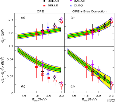
Figure 7: The first and second moments of the photon energy in $B\to\gamma X$ compared to OPE predictions without and with bias corrections. The inner band indicates the experimental uncertainties only; the outer bands add the theoretical ones; from Ref.[66]

Fig.7 shows data for the average photon energy and its variance for different lower cuts on the photon energy from CLEO, BABAR and BELLE compared to the OPE predictions without and with bias corrections on the left and right, respectively. The comparison shows the need for those bias corrections and them being under computational control over a sizable range of $E_{cut}$. Even more important than providing us with possibly more accurate values for $m_{b}$ and $\mu_{\pi}^{2}$, these studies enhance confidence in our theoretical tools.

These findings lead to the following conclusions: (i) As far as theory is concerned there is a high premium on keeping the cuts as low as possible. (ii) Such cuts introduce biases in the HQP values extracted from the truncated moments; yet within a certain range of the cut variables those biases can be corrected for and thus should not be used to justify inflating the theoretical uncertainties. (iii) In any case measuring the moments as functions of the cuts provides powerful cross checks for our theoretical control.

‘Let a Thousand Blossoms Bloom’: Several suggestions have been made for cuts to suppress the $b\to c$ background to managable proportions. None provides a panacea. The most straightforward one is to focus on the lepton energy endpoint region; however it captures merely a small fraction of the total $b\to u$ rate, which can be estimated only with considerable model dependance. This model sensitivity can be moderated with information on the heavy quark distribution function inferred from $B\to\gamma X$. Furthermore weak annihilation contributes only in the endpoint region and with different weight in $B_{d}$ and $B_{u}$ decays [59]. Thus the lepton spectra have to be measured separately for charged and neutral $B$ decays.

Measuring the hadronic recoil mass spectrum up to a maximal value $M_{X}^{\rm max}$ captures the lion share of the $b\to u$ rate if $M_{X}^{\rm max}$ is above 1.5 GeV; yet it is still vulnerable to theoretical uncertainties in the very low $q^{2}$ region. This problem can be addressed in two different ways: adopting Alexander the Great’s treatment of the Gordian knot one can impose a lower cut on $q^{2}$ or one can describe the low $q^{2}$ region with the help of the measured energy spectrum in $B\to\gamma X$ for 1.8 GeV $\leq E_{\gamma}\leq$ 2.0 GeV. Alternatively one can apply a combination of cuts. Studying $B_{d}$ and $B_{u}$ decays is still desirable, yet not as essential as for the previous case.

In any case one should not restrict oneself to a fixed cut, but vary the latter over some reasonable range and analyze to which degree theory can reproduce this cut dependence to demonstrate control over the uncertainties.

There is not a single ‘catholic’ path to the promised land of a precise value for $|V(ub)|$; presumably many paths will have to be combined [86]. Yet it seems quite realistic that the error can be reduced to about 5 % over the next few years.

0.2.5 Summary of Lect. II

As explained in Lect. I while CKM forces are generated by the exchange of gauge bosons, its couplings involve elements of the CKM matrix. Yet those originate in the elements of the up- and down-type quark mass matrices. Thus the CKM parameters are intrinsically connected with one of the central mysteries of the SM, namely the generation in particular of fermion masses and family replication. Furthermore the hierarchy in the quark masses and the likewise hierarchical pattern of the CKM matrix elements strongly hints at some deeper level of dynamics about which we are quite ignorant. Nevertheless CKM theory with its mysterious origins has proved itself to be highly successful in describing even quantitatively a host of phenomena occurring over a wide array of scales. It lead to the ‘Paradigm of Large CP Violation in $B$ Decays as a prediction in the old-fashioned sense; i.e., predictions were made well before data of the required sensitivity existed. From the observation of a tiny and shy phenomenon – CP violation in $K_{L}$ decays on the ${\cal O}(10^{-3})$ level – it predicted without ‘plausible deniability’ almost ubiquitous manifestations of CP violation about two orders of magnitude larger in $B$ decays. This big picture has been confirmed now in qualitative as well as impressively quantitative agreement with SM predictions:

• Two CP insensitive observables, namely $|V(ub)/V(cb)|$ and $\Delta M_{B_{d}}/\Delta M_{B_{s}}$, imply that CP violation has to exist and in a way that at present is fully consistent with the measurements of $\epsilon$ and sin$2\phi_{1}$ and others.

• Time dependent CP asymmetries in the range of several $\times$ 10 % have been established in $B_{d}\to\psi K_{S}$, $\pi^{+}\pi^{-}$ and $\eta^{\prime}K_{S}$ with several others on the brink of being found.

• Direct CP violation of about 10% or even larger have been discovered in $B_{d}\to\pi^{+}\pi^{-}$ and $K^{-}\pi^{+}$.

• The first significant sign of CP violation in a charged meson has surfaced in $B^{\pm}\to K^{\pm}\rho^{0}$.

• The optimists among us might discern the first signs of tension between data and the predictions of CKM theory in $|V(ub)/V(cb)|$ & $\Delta M_{B_{d}}/\Delta M_{B_{s}}$ vs. sin$2\phi_{1}$ and in the CP asymmetries in $b\to sq\bar{q}$ vs. $b\to c\bar{c}s$ driven transitions.

For all these successes it is quite inappropriate to refer anymore to CKM theory as an ‘ansatz’ with the latter’s patronizing flavour . Instead I would characterize these developments as "the expected triumph of peculiar theory". However, as explained in Lect. III, it makes great sense – actually it is mandatory to search for its phenomenological limitations in future even more sensitive data sets. This will require great advances in experimental sensitivity – I have no doubt about their feasibility – and further progress in out quantitative theoretical control over heavy flavour decays. I have presented some case studies, which give reason for optimism in this area as well. An essential element there is the availability of a comprehensive set of high quality data: among other things they provide the motivation for theorists to sharpen their tools, and they allow us to defend our estimates of uncertainties rather than merely state them.

I will indulge myself in three more ‘cultural’ conclusions:

• The aforementioned "CKM Paradigm of Large CP Violation in $B$ Decays" is due to the confluence of several favourable, yet a priori less than likely factors that must be seen as gifts from nature who had

  • arranged for a huge top mass,

  • a "long" $B$ lifetime,

  • the $\Upsilon(4S)$ resonance being above the $B\bar{B}$, yet below the $B\bar{B}^{*}$ thresholds and

  • regaled us previously with charm hadrons, which prompted the development detectors with an effective resolution that is needed to track $B$ decays.

• ‘Quantum mysteries’ like EPR correlations with their intrinsic non-local features were essential for observing CP violation involving $B_{d}-\bar{B}_{d}$ oscillations in $\Upsilon(4S)\to B_{d}\bar{B}_{d}$ and to establish that indeed there is T violation commensurate with CP violation.

• While hadronization is not easily brought under quantitative theoretical control it enhances greatly observable CP asymmetries and can provide most valuable cross checks for our interpretation of data.

0.3 Lecture III: Probing the Flavour Paradigm of the Emerging New Standard Model

0.3.1 On the Incompleteness of the SM

As described in the previous lectures the SM has scored novel – i.e., qualitatively new – successes in the last few years in the realm of flavour dynamics. Due to the very peculiar structure of the latter they have to be viewed as amazing. Yet even so the situation can be characterized with a slightly modified quote from Einstein:

"We know a lot – yet understand so little."

I.e., these successes do not invalidate the general arguments in favour of the SM being incomplete – the search for New Physics is as mandatory as ever.

You have heard about the need to search for New Physics before and what the outcome has been of such efforts so far, have you not? And it reminds you of a quote by Samuel Beckett:

"Ever tried? Ever failed?

No matter.

Try again. Fail again. Fail better."

Only an Irishman can express profound skepticism concerning the world in such a poetic way. Beckett actually spent most of his life in Paris, since Parisians like to listen to someone expressing such a world view, even while they do not share it. Being in the service of Notre Dame du Lac, the home of the ‘Fighting Irish’, I cannot just ignore such advice.

My colleague and friend Antonio Masiero likes to say: "You have to be lucky to find New Physics." True enough – yet let me quote someone who just missed by one year being a fellow countryman of Masiero, namely Napoleon, who said: "Being lucky is part of the job description for generals." Quite seriously I think that if you as an high energy physicist do not believe that someday somewhere you will be a general – maybe not in a major encounter, but at least in a skirmish – then you are frankly in the wrong line of business.

My response to these concerns is: "Cheer up – we know there is New Physics – we will not fail forever!" I will marshall the arguments – compelling ones in my judgment – that point to the existence of New Physics.

Theoretical Shortcomings

These arguments have been given already in the beginning of Lecture I.

• Quantization of electric charge: While electric charge quantization

  $$Q_{e}=3Q_{d}=-\frac{3}{2}Q_{u}$$ (243)

  is an essential ingredient of the SM – it allows to vitiate the ABJ anomaly – it does not offer any understanding. It would naturally be explained through Grand Unification at very high energy scales implemented through, e.g., $SO(10)$ gauge dynamics. I call this the ‘guaranteed New Physics’.

• Family Replication and CKM Structure: We infer from the observed width of $Z^{0}$ decays that there are three (light) neutrino species. The hierarchical pattern of CKM parameters as revealed by the data is so peculiar as to suggest that some other dynamical layer has to underlie it. I refer to it as ‘strongly suspected New Physics’ or ssNP. We are quite in the dark about its relevant scales. Saying we pin our hopes for explaining the family replication on Super-String or M theory is a scholarly way of saying we have hardly a clue what that ssNP is.

• Electroweak Symmetry Breaking and the Gauge Hierarchy: What are the dynamics driving the electroweak symmetry breaking of $SU(2)_{L}\times U(1)\to U(1)_{QED}$. How can we tame the instability of Higgs dynamics with its quadratic mass divergence? I find the arguments compelling that point to New Physics at the $\sim 1$ TeV scale – like low-energy SUSY; therefore I call it the ‘confidently predicted’ New Physics or cpNP.

• Furthermore the more specific ‘Strong CP Problem’ of QCD has not been resolved. Similar to the other shortcomings it is a purely theoretical problem in the sense that the offending coefficient for the P and CP odd operator $\tilde{G}\cdot G$ can be fine-tuned to zero , see Sect.0.1.1, – yet in my eyes that is not a flaw.

Experimental Signs

Strong, albeit not conclusive (by itself) evidence for neutrino oscillations comes from the KAMLAND and K2K experiments in Japan studying the evolution of neutrino beams on earth.

Yet compelling experimental evidence for the SM being incomplete comes from ‘heavenly signals’, namely from astrophysics and cosmology.

• The Baryon Number of the Universe: one finds only about one baryon per $10^{9}$ photons with the latter being mostly in the cosmic background radiation; there is no evidence for primary antimatter.

  $\ominus$ We know standard CKM dynamics is irrelevant for the Universe’s baryon number.

  $\oplus$ Therefore New Physics has to exist.

  $\oplus$ The aforementioned New CP Paradigm tells us that CP violating phases can be large.

• Dark Matter: Analysis of the rotation curves of stars and galaxies reveal that there is a lot more ‘stuff’ – i.e. gravitating agents – out there than meets the eye. About a quarter of the gravitating agents in the Universe are such dark matter, and they have to be mostly nonbaryonic.

  $\oplus$ The SM has no candidate for it.

• Solar and Atmospheric $\nu$ Anomalies: The sun has been ‘seen’ by Super-Kamiokande in the light of neutrinos, as shown in Fig.8. Looking carefully one realizes that the sun looks paler than it should: more than half of the originally produced $\bar{\nu}_{e}$ disappear on the way to the earth by changing their identity. Muon neutrinos produced in the atmosphere perform a similar disappearance act.

  

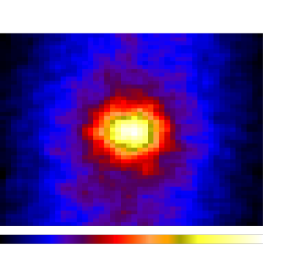
  Figure 8: The sun in the light of its neutrino emission as seen by the Super-Kamiokande detector; from Ref.[87]

  These disappearances have to be attributed predominantly to neutrino oscillations (rather than neutrino decays). This requires neutrinos to carry nondegenerate masses.

• Dark Energy: Type 1a supernovae are considered ‘standard candles’; i.e. considering their real light output known allows to infer their distance from their apparent brightness. When in 1998 two teams of researchers studied them at distance scales of about five billion light years, they found them to be fainter as a function of their redshift than what the conventional picture of the Universe’s decelerating expansion would yield. Unless gravitational forces are modified over cosmological distances, one has to conclude the Universe is filled with an hitherto completely unknown agent accelerating the expansion. A tiny, yet non-zero cosmological constant would apparently ‘do the trick’ – yet it would raise more fundamental puzzles.

These heavenly signals are unequivocal in pointing to New Physics, yet leave wide open the nature of this New Physics.

Thus we can be assured that New Physics exists ‘somehow’ ‘somewhere’, and quite likely even ‘nearby’, namely around the TeV scale; above I have called the latter cpNN. The LHC program and the Linear Collider project are justified – correctly – to conduct campaigns for cpNP. That is unlikely to shed light on the ssNP, though it might. Likewise I would not count on a comprehensive and detailed program of heavy flavour studies to shed light on the ssNP behind the flavour puzzle of the SM. Yet the argument is reasonably turned around: such a program will be essential to elucidate salient features of the cpNP by probing the latter’s flavour structure and having sensitivity to scales of order 10 TeV. One should keep in mind the following: one very popular example of cpNP is supersymmetry; yet it represents an organizing principle much more than even a class of theories. I find it unlikely we can infer all required lessons by studying only flavour diagonal transitions. Heavy flavour decays provide a powerful and complementary probe of cpNP. Their potential to reveal something about the ssNP is a welcome extra not required for justifying efforts in that direction.

Accordingly I see a dedicated heavy flavour program as an essential complement to the studies pursued at the high energy frontier at the TEVATRON, LHC and hopefully ILC. I will illustrate this assertion in the remainder of this lecture.

0.3.2 $\Delta S\neq 0$ – the ‘Established Hero’

The chapter on $\Delta S\neq 0$ transitions is a most glorious one in the history of particle physics, as sketched in Table 5.

Observation	Lesson learnt
$\tau-\theta$ Puzzle	P violation
production rate $\gg$ decay rate	concept of families
suppression of flavour changing neutral currents	GIM mechanism & existence of charm
$K_{L}\to\pi\pi$	CP violation & existence of top

Table 5: On the History of $\Delta S\neq 0$ Studies

We should note that all these features, which now are pillars of the SM, were New Physics at that time!

Future ‘Bread & Butter’ Topics

Detailed studies of radiative decays like $K\to\pi\gamma\gamma$ and $K\to\pi\pi\gamma$ will allow deeper probes of chiral perturbation theory. The lessons thus obtained might lead to a better treatment of long distance dynamics’ impact on the $\Delta I=1/2$ rule, $\Delta M_{K}$, $\epsilon_{K}$ and $\epsilon^{\prime}$.

The ‘Dark Horse’

The T odd moment (see Sect.0.1.2)

$${\rm Pol}_{\perp}(\mu)\equiv\frac{\langle\vec{s}(\mu)\cdot(\vec{p}(\mu)\times\vec{p}(\pi))\rangle}{|\vec{p}(\mu)\times\vec{p}(\pi)|}$$ (244)

measured in $K^{+}\to\mu^{+}\nu\pi^{0}$ would

• represent genuine T violation (as long as it exceeded the order $10^{-6}$ level) and

• constitute prima facie evidence for CP violation in scalar dynamics.

‘Heresy’

The large T odd correlation found in $K_{L}\to\pi^{+}\pi^{-}e^{+}e^{-}$ for the relative orientation of the $\pi^{+}\pi^{-}$ and $e^{+}e^{-}$ decay planes, see the discussion below in Sect.0.3.3, is fully consistent with a T violation as inferred from the CP violation expressed through $\epsilon_{K}$ – yet it does not prove it [94]. In an unabashedly contrived scenario – something theorists usually avoid at great pains – one could reconcile the data on $K_{L}\to\pi^{+}\pi^{-}e^{+}e^{-}$ with T invariance without creating a conflict with known data. Yet the CPT violation required in this scenario would have to surface through [94]

$$\frac{\Gamma(K^{+}\to\pi^{+}\pi^{0})-\Gamma(K^{-}\to\pi^{-}\pi^{0})}{\Gamma(K^{+}\to\pi^{+}\pi^{0})+\Gamma(K^{-}\to\pi^{-}\pi^{0})}>10^{-3}$$ (245)

The ‘Second Trojan War’: $K\to\pi\nu\bar{\nu}$

According to Greek Mythology the Trojan War described in Homer’s Iliad was actually the second war over Troja. In a similar vein I view the heroic campaign over $K^{0}-\bar{K}^{0}$ oscillations – $\Delta M_{K}$, $\epsilon_{K}$ and $\epsilon^{\prime}$ – as a first one to be followed by a likewise epic struggle over the two ultra-rare modes $K^{+}\to\pi^{+}\nu\bar{\nu}$ and $K_{L}\to\pi^{0}\nu\bar{\nu}$. This campaign has already been opened through the observation of the first through three events very roughly as expected within the SM. The second one, which requires CP violation for its mere existence, so far remains unobserved at a level well above SM predictions. These reactions are like ‘standard candles’ for the SM: their rates are functions of $V(td)$ with a theoretical uncertainty of about 5% and 2% respectively, which is mainly due to the uncertainty in the charm quark mass.

While their rates could be enhanced by New Physics greatly over their SM expectation, I personally find that somewhat unlikely for various reasons. Therefore I suggest one should aim for collecting ultimately about 1000 events of these modes to extract the value of $V(td)$ and/or identify likely signals of New Physics.

0.3.3 The ‘King Kong’ Scenario for New Physics Searches

This scenario can be formulated as follows: "One is unlikely to encounter King Kong; yet once it happens one will have no doubt that one has come across something quite out of the ordinary!"

What it means can be best illustrated with the historical precedent of $\Delta S\neq 0$ studies sketched above: the existence of New Physics can unequivocally be inferred if there is a qualitative conflict between data and expectation; i.e., if a theoretically ‘forbidden’ process is found to proceed nevertheless – like in $K_{L}\to\pi\pi$ – or the discrepancy between expected and observed rates amounts to several orders of magnitude – like in $K_{L}\to\mu^{+}\mu^{-}$ or $\Delta M_{K}$. This does not mean that the effects are large or straightforward to discover – only that they are much larger than the truly minute SM effects.

History might repeat itself in the sense that future measurements might reveal such qualitative conflicts, where the case for the manifestation of New Physics is easily made. This does not mean that such measurements will be easy – far from it, as will become obvious.

I have already mentioned one potential candidate for revealing such a qualitative conflict, namely the muon transverse polarization in $K_{\mu 3}$ decays.

Electric Dipole Moments

The energy shift of a system placed inside a weak electric field can be expressed through an expansion in terms of the components of that field $\vec{E}$:

$$\Delta{\cal E}=d_{i}E_{i}+d_{ij}E_{i}E_{j}+{\cal O}(E^{3})$$ (246)

The coefficients $d_{i}$ of the term linear in the electric field form a vector $\vec{d}$, called an electric dipole moment (EDM). For a non-degenerate system – it does not have to be elementary – one infers from symmetry considerations that this vector has to be proportional to that systems spin:

$$\vec{d}\propto\vec{s}$$ (247)

Yet, since

$$E_{i}\stackrel{{\scriptstyle{\bf T}}}{{\to}}E_{i}\;\;,\;\;s_{i}\stackrel{{\scriptstyle{\bf T}}}{{\to}}-s_{i}$$ (248)

under time reversal T, a non-vanishing EDM constitutes T violation.

No EDM has been observed yet; the upper bounds of the neutron and electron EDM read as follows [95]:

$$d_{N} < 5\cdot 10^{-26}\;{\rm e\,cm}\;\;\;{\rm[from\;ultracold\;neutrons]}$$ (249)

$$d_{e} < 1.5\cdot 10^{-27}\;{\rm e\,cm}\;\;\;{\rm[from\;atomic\;EDM]}$$ (250)

The experimental sensitivity achieved can be illustrated as follows: (i) An neutron EDM of $5\cdot 10^{-26}$ e cm of an object with a radius $r_{N}\sim 10^{-13}$ cm scales to a displacement of about 7 micron, i.e. less than the width of human hair, for an object of the size of the earth. (ii) Expressing the uncertainty in the measurement of the electron’s magnetic dipole moment – $\delta((g-2)/2)\sim 10^{-11}$ in analogy to its EDM, one finds a sensitivity level of $\delta(F_{2}(0)/2m_{e})\sim 2\cdot 10^{-22}$ e cm compared to $d_{e}<2\cdot 10^{-26}$ e cm.

Despite the tremendous sensitivity reached these numbers are still several orders of magnitude above what is expected in CKM theory:

$$d_{N}^{CKM} \leq 10^{-30}\;{\rm e\,cm}$$ (251)

$$d_{e}^{CKM} \leq 10^{-36}\;{\rm e\,cm}\;,$$ (252)

where in $d_{N}^{CKM}$ I have ignored any contribution from the strong CP problem. These numbers are so tiny for reasons very specific to CKM theory, namely its chirality structure and the pattern in the quark and lepton masses. Yet New Physics scenarios with right-handed currents, flavour changing neutral currents, a non-minimal Higgs sector, heavy neutrinos etc. are likely to generate considerably larger numbers: $10^{-28}-10^{-26}$ e cm represents a very possible range there quite irrespective of whether these new forces contribute to $\epsilon_{K}$ or not. This range appears to be within reach in the foreseeable future. There is a vibrant multiprong program going on at several places. Such experiments while being of the ‘table top’ variety require tremendous efforts, persistence and ingenuity – yet the insights to be gained by finding a nonzero EDM somewhere are tremendous.

Charm Decays

Charm dynamics is often viewed as physics with a great past – it was instrumental in driving the paradigm shift from quarks as mathematical entities to physical objects and in providing essential support for accepting QCD as the theory of the strong interactions – yet one without a future since the electroweak phenomenology for $\Delta C\neq 0$ transitions is decidedly on the ‘dull’ side: ‘known’ CKM parameters, slow $D^{0}-\bar{D}^{0}$ oscillations, small CP asymmetries and extremely rare loop driven decays.

Yet more thoughtful observers have realized that the very ‘dullness’ of the SM phenomenology for charm provides us with a dual opportunity, namely to

• probe our quantitative understanding of QCD’s nonperturbative dynamics thus calibrating our theoretical tools for $B$ decays and

• perform almost ‘zero-background’ searches for New Physics.

However the latter statement of ‘zero-background’ has to be updated carefully since experiments over the last ten years have bounded the oscillation parameters $x_{D}$, $y_{D}$ to fall below very few % and direct CP asymmetries below several %. While New Physics signals can still exceed SM predictions on CP asymmetries by orders of magnitude, they might not be large in absolute terms, as specified later [96].

One should take note that charm is the only up-type quark allowing the full range of probes for New Physics, including flavour changing neutral currents: while top quarks do not hadronize [50], in the $u$ quark sector you cannot have $\pi^{0}-\pi^{0}$ oscillations and many CP asymmetries are already ruled out by CPT invariance. My basic contention is the following: Charm transitions are a unique portal for obtaining a novel access to flavour dynamics with the experimental situation being a priori favourable (except for the lack of Cabibbo suppression)!

I will sketch such searches for New Physics in the context of $D^{0}-\bar{D}^{0}$ oscillations and CP violation.

1. Like for $K^{0}$ and $B^{0}$ mesons the oscillations of $D^{0}$ mesons represent a subtle quantum mechanical phenomenon of practical importance: it provides a probe for New Physics, albeit an ambiguous one, and constitutes an important ingredient for CP asymmetries arising in $D^{0}$ decays due to New Physics.

   In qualitative analogy to the $K^{0}$ and $B^{0}$ cases these phenomena can be characterized by two quantities, namely $x_{D}=\frac{\Delta M_{D}}{\Gamma_{D}}$ and $y_{D}=\frac{\Delta\Gamma_{D}}{2\Gamma_{D}}$. Oscillations are slowed down in the SM due to GIM suppression and $SU(3)_{fl}$ symmetry. Comparing a conservative SM bound with the present data

   $$x_{D}(SM),y_{D}(SM)<{\cal O}(0.01)\;\;vs.\;\;\left.x_{D}\right|_{exp}<0.03\;,\;\;\left.y_{D}\right|_{exp}=0.01\pm 0.005$$ (253)

   we conclude that the search has just now begun. There exists a considerable literature – yet typically with several ad-hoc assumptions concerning the nonperturbative dynamics. It is widely understood that the usual quark box diagram is utterly irrelevant due to its untypically severe GIM suppression $(m_{s}/m_{c})^{4}$. A systematic analysis based on an OPE treatment has been given in Ref.[88] in terms of powers of $1/m_{c}$ and $m_{s}$. Contributions from higher-dimensional operators with a much softer GIM reduction of $(m_{s}/\mu_{had})^{2}$ (even $m_{s}/\mu_{had}$ terms could arise) due to ‘condensate’ terms in the OPE yield

   $$\left.x_{D}(SM)\right|_{OPE},\;\left.y_{D}(SM)\right|_{OPE}\sim{\cal O}(10^{-3})\;.$$ (254)

   Ref.[89] finds very similar numbers, albeit in a quite different approach.

   While one predicts similar numbers for $x_{D}(SM)$ and $y_{D}(SM)$, one should keep in mind that they arise in very different dynamical environments. $\Delta M_{D}$ is generated from off-shell intermediate states and thus is sensitive to New Physics, which could produce $x_{D}\sim{\cal O}(10^{-2})$. $\Delta\Gamma_{D}$ on the other hand is shaped by on-shell intermediate states; while it is hardly sensitive to New Physics, it involves much less averaging or ‘smearing’ than $\Delta M_{D}$ making it thus much more vulnerable to violations of quark-hadron duality. Observing $y_{D}\sim 10^{-3}$ together with $x_{D}\sim 0.01$ would provide intriguing, though not conclusive evidence for New Physics, while $y_{D}\sim 0.01\sim x_{D}$ would pose a true conundrum for its interpretation.

2. Since the baryon number of the Universe implies the existence of New Physics in CP violating dynamics, it would be unwise not to undertake dedicated searches for CP asymmetries in charm decays, where the ‘background’ from known physics is small: within the SM the effective weak phase is highly diluted, namely $\sim{\cal O}(\lambda^{4})$, and it can arise only in singly Cabibbo suppressed transitions, where one expects them to reach the 0.1 % level; significantly larger values would signal New Physics. Any asymmetry in Cabibbo allowed or doubly suppressed channels requires the intervention of New Physics – except for $D^{\pm}\to K_{S}\pi^{\pm}$ [61], where the CP impurity in $K_{S}$ induces an asymmetry of $3.3\cdot 10^{-3}$. Several facts actually favour such searches: strong phase shifts required for direct CP violation to emerge in partial widths are in general large as are the branching ratios into relevant modes; finally CP asymmetries can be linear in New Physics amplitudes thus enhancing sensitivity to the latter. As said above, the benchmark scale for KM asymmetries in singly Cabibbo suppressed partial widths is $0.1\%$. This does not exclude the possibility that CKM dynamics might exceptionally generate an  asymmetry as ‘large’ as 1% in some special cases. It is therefore essential to analyze a host of channels.

   Decays to final states of more than two pseudoscalar or one pseudoscalar and one vector meson contain more dynamical information than given by their widths; their distributions as described by Dalitz plots or T-odd moments can exhibit CP asymmetries that can be considerably larger than those for the width. Final state interactions while not necessary for the emergence of such effects, can fake a signal; yet that can be disentangled by comparing T-odd moments for CP conjugate modes. I view this as a very promising avenue, where we still have to develop the most effective analysis tools for small asymmetries.

   CP violation involving $D^{0}-\bar{D}^{0}$ oscillations can be searched for in final states common to $D^{0}$ and $\bar{D}^{0}$ decays like CP eigenstates – $D^{0}\to K_{S}\phi$, $K^{+}K^{-}$, $\pi^{+}\pi^{-}$ – or doubly Cabibbo suppressed modes – $D^{0}\to K^{+}\pi^{-}$. The CP asymmetry is controlled by sin$\Delta m_{D}t$ $\cdot$ Im$(q/p)\bar{\rho}(D\to f)$; within the SM both factors are small, namely $\sim{\cal O}(10^{-3})$, making such an asymmetry unobservably tiny – unless there is New Physics! One should note that this observable is linear in $x_{D}$ rather than quadratic as for CP insensitive quantities. $D^{0}-\bar{D}^{0}$ oscillations, CP violation and New Physics might thus be discovered simultaneously in a transition.

   One wants to reach the level at which SM effects are likely to emerge, namely down to time-dependent CP asymmetries in $D^{0}\to K_{S}\phi$, $K^{+}K^{-}$, $\pi^{+}\pi^{-}$ [$K^{+}\pi^{-}$] down to $10^{-5}$ [$10^{-4}$] and direct CP asymmetries in partial widths and Dalitz plots down to $10^{-3}$.

CP Asymmetries in Final State Distributions

So far CP violation has surfaced in time-integrated or time-dependent partial widths with one notable exception. A large T odd moment was found in the rare $K_{L}$ mode – BR$(K_{L}\rightarrow\pi^{+}\pi^{-}e^{+}e^{-})=(3.32\pm 0.14\pm 0.28)\cdot 10^{-7}$: With $\phi$ defined as the angle between the planes spanned by the two pions and the two leptons in the $K_{L}$ restframe:

$$\phi\equiv\angle(\vec{n}_{l},\vec{n}_{\pi})$$

$$\vec{n}_{l}=\vec{p}_{e^{+}}\times\vec{p}_{e^{-}}/|\vec{p}_{e^{+}}\times\vec{p}_{e^{-}}|\;,\;\vec{n}_{\pi}=\vec{p}_{\pi^{+}}\times\vec{p}_{\pi^{-}}/|\vec{p}_{\pi^{+}}\times\vec{p}_{\pi^{-}}|$$ (255)

one analyzes the decay rate as a function of $\phi$:

$$\frac{d\Gamma}{d\phi}=\Gamma_{1}{\rm cos}^{2}\phi+\Gamma_{2}{\rm sin}^{2}\phi+\Gamma_{3}{\rm cos}\phi\,{\rm sin}\phi$$ (256)

Since

$${\rm cos}\phi\,{\rm sin}\phi=(\vec{n}_{l}\times\vec{n}_{\pi})\cdot(\vec{p}_{\pi^{+}}+\vec{p}_{\pi^{-}})(\vec{n}_{l}\cdot\vec{n}_{\pi})/|\vec{p}_{\pi^{+}}+\vec{p}_{\pi^{-}}|$$ (257)

one notes that

$${\rm cos}\phi\,{\rm sin}\phi\;\;\;\stackrel{{\scriptstyle{\bf T},{\bf CP}}}{{\longrightarrow}}\;\;\;-\;{\rm cos}\phi\,{\rm sin}\phi$$ (258)

under both T  and CP transformations; i.e. the observable $\Gamma_{3}$ represents a T - and CP -odd correlation. It can be projected out by comparing the $\phi$ distribution integrated over two quadrants:

$$A=\frac{\int_{0}^{\pi/2}d\phi\frac{d\Gamma}{d\phi}-\int_{\pi/2}^{\pi}d\phi\frac{d\Gamma}{d\phi}}{\int_{0}^{\pi}d\phi\frac{d\Gamma}{d\phi}}=\frac{2\Gamma_{3}}{\pi(\Gamma_{1}+\Gamma_{2})}$$ (259)

It was first measured by KTEV and then confirmed by NA48 [95]:

$$A=(13.7\pm 1.5)\%\,.$$ (260)

$A\neq 0$ is induced by $\epsilon_{K}$, the CP violation in the $K^{0}-\bar{K}^{0}$ mass matrix, leading to the prediction [97]

$$A=(14.3\pm 1.3)\%\,.$$ (261)

The observed value for the T odd moment $A$ is fully consistent with T violation. Yet $A\neq 0$ by itself does not establish T violation [94].

One should note that this sizable forward-backward asymmetry is driven by the tiny quantity $|\eta_{+-}|\simeq 0.0023$, which can be understood. For $K_{L}\to\pi^{+}\pi^{-}e^{+}e^{-}$ is driven by the two sub-processes

$$K_{L} \stackrel{{\scriptstyle\not{{\bf CP}}\&\Delta S=1}}{{\longrightarrow}}\pi^{+}\pi^{-}\stackrel{{\scriptstyle E1}}{{\longrightarrow}}\pi^{+}\pi^{-}\gamma^{*}\to\pi^{+}\pi^{-}e^{+}e^{-}$$ (262)

$$K_{L} \stackrel{{\scriptstyle M1\&\Delta S=1}}{{\longrightarrow}}\pi^{+}\pi^{-}\gamma^{*}\to\pi^{+}\pi^{-}e^{+}e^{-}\;,$$ (263)

where the first reaction is suppressed, since it requires CP violation in $K_{L}\to 2\pi$, and the second one, since it involves an $M1$ transition. Those two a priori very different suppression mechanisms happen to yield comparable amplitudes, which thus generate sizable interference. The price one pays is the small branching ratio.

$D$ decays can be treated in an analogous way. Consider the Cabibbo suppressed channel

$$\stackrel{{\scriptstyle(-)}}{{D}}\to K\bar{K}\pi^{+}\pi^{-}$$ (264)

and define by $\phi$ now the angle between the $K\bar{K}$ and $\pi^{+}\pi^{-}$ planes. Then one has

$$\frac{d\Gamma}{d\phi}(D\to K\bar{K}\pi^{+}\pi^{-}) = \Gamma_{1}{\rm cos}^{2}\phi+\Gamma_{2}{\rm sin}^{2}\phi+\Gamma_{3}{\rm cos}\phi{\rm sin}\phi$$ (265)

$$\frac{d\Gamma}{d\phi}(\bar{D}\to K\bar{K}\pi^{+}\pi^{-}) = \bar{\Gamma}_{1}{\rm cos}^{2}\phi+\bar{\Gamma}_{2}{\rm sin}^{2}\phi+\bar{\Gamma}_{3}{\rm cos}\phi{\rm sin}\phi$$ (266)

As before the partial width for $D[\bar{D}]\to K\bar{K}\pi^{+}\pi^{-}$ is given by $\Gamma_{1,2}[\bar{\Gamma}_{1,2}]$; $\Gamma_{1}\neq\bar{\Gamma}_{1}$ or $\Gamma_{2}\neq\bar{\Gamma}_{2}$ represents direct CP violation in the partial width. $\Gamma_{3}\&\bar{\Gamma}_{3}$ constitute T odd correlations. By themselves they do not necessarily indicate CP violation, since they can be induced by strong final state interactions. However

$$\Gamma_{3}\neq\bar{\Gamma}_{3}\;\;\Longrightarrow{\bf CP}~{}{\rm violation!}$$ (267)

It is quite possible or even likely that a difference in $\Gamma_{3}$ vs. $\bar{\Gamma}_{3}$ is significantly larger than in $\Gamma_{1}$ vs. $\bar{\Gamma}_{1}$ or $\Gamma_{2}$ vs. $\bar{\Gamma}_{2}$. Furthermore one can expect that differences in detection efficiencies can be handled by comparing $\Gamma_{3}$ with $\Gamma_{1,2}$ and $\bar{\Gamma}_{3}$ with $\bar{\Gamma}_{1,2}$. A pioneering search for such an effect has been undertaken by FOCUS [100].

CP Violation in the Lepton Sector

I find the conjecture that baryogenesis is a secondary phenomenon driven by primary leptogenesis a most intriguing and attractive one also for philosophical reasons . Yet then it becomes mandatory to search for CP violation in the lepton sector in a most dedicated fashion.

In Sect. 0.3.3 I have sketched the importance of measuring electric dipole moments as accurately as possible. The electron’s EDM is a most sensitive probe of CP violation in leptodynamics. Comparing the present experimental and CKM upper bounds, respectively

$$d_{e}^{exp}\leq 1.5\cdot 10^{-27}\;\;{\rm e\;cm}\;\;\;vs.\;\;\;d_{e}^{CKM}\leq 10^{-36}\;\;{\rm e\;cm}$$ (268)

we see there is a wide window of several orders of magnitude, where New Physics could surface in an unambiguous way. This observation is reinforced by the realization that New Physics scenarios can naturally generate $d_{e}>10^{-28}$e cm, while of only secondary significance in $\epsilon_{K}$, $\epsilon^{\prime}$ and sin$2\phi_{i}$.

The importance that at least part of the HEP community attributes to finding CP violation in leptodynamics is best demonstrated by the efforts contemplated for observing CP asymmetries in neutrino oscillations. Clearly hadronization will be the least of the concerns, yet one has to disentangle genuine CP violation from matter enhancements, since the neutrino oscillations can be studied only in a matter, not an antimatter environment. Our colleagues involved in such endeavours will rue their previous complaints about hadronization and remember the wisdom of an ancient Greek saying:

"When the gods want to really harm you, they fulfill your wishes."

The Decays of $\tau$ Leptons – the Next ‘Hero Candidate’

Like charm hadrons the $\tau$ lepton is often viewed as a system with a great past, but hardly a future. Again I think this is a very misguided view and I will illustrate it with two examples.

Searching for $\tau^{\pm}\to\mu^{\pm}\mu^{+}\mu^{-}$ (and its variants) – processes forbidden in the SM – is particularly intriguing, since it involves only ‘down-type’ leptons of the second and third family and is thus the complete analogy of the quark lepton process $b\to s\bar{s}s$ driving $B_{s}\to\phi K_{S}$, which has recently attracted such strong attention. Following this analogy literally one guestimates ${\rm BR}(\tau\to 3\mu)\sim 10^{-8}$ to be compared with the present bound from BELLE

$${\rm BR}(\tau\to 3\mu)\leq 2\cdot 10^{-7}\;.$$ (269)

It would be very interesting to know what the $\tau$ production rate at the hadronic colliders is and whether they could be competitive or even superior with the $B$ factories in such a search.

In my judgment $\tau$ decays – together with electric dipole moments for leptons and possibly $\nu$ oscillations referred to above – provide the best stage to search for manifestations of CP breaking leptodynamics.

The most promising channels for exhibiting CP asymmetries are $\tau\to\nu K\pi$, since due to the heaviness of the lepton and quark flavours they are most sensitive to nonminimal Higgs dynamics, and they can show asymmetries also in the final state distributions rather than integrated rates [91].

There is also a unique opportunity in $e^{+}e^{-}\to\tau^{+}\tau^{-}$: since the $\tau$ pair is produced with its spins aligned, the decay of one $\tau$ can ‘tag’ the spin of the other $\tau$. I.e., one can probe spin-dependent CP asymmetries with unpolarized beams. This provides higher sensitivity and more control over systematic uncertainties.

I feel these features are not sufficiently appreciated even by proponents of Super-B factories. It has been recently pointed [92] out that based on known physics one can actually predict a CP asymmetry:

$$\frac{\Gamma(\tau^{+}\to K_{S}\pi^{+}\overline{\nu})-\Gamma(\tau^{-}\to K_{S}\pi^{-}\nu)}{\Gamma(\tau^{+}\to K_{S}\pi^{+}\overline{\nu})+\Gamma(\tau^{-}\to K_{S}\pi^{-}\nu)}=(3.27\pm 0.12)\times 10^{-3}$$ (270)

due to $K_{S}$’s preference for antimatter.

0.3.4 Future Studies of $B_{u,d}$ Decays

The successes of CKM theory to describe flavour dynamics do not tell us at all that New Physics does not affect $B$ decays; the message is that typically we cannot count on a numerically massive impact there. Shifting an asymetry by, say, ten percentage points – for example from 40 % to 50 % – might already be on the large side. Thus our aim has to be to aim for uncertainties that do not exceed a few percent.

The discussion given in Lect. II shows that an integrated luminosity of 1 $ab^{-1}$ at the $B$ factories will fall short of such a goal for $B_{d}\to\pi\pi$, $B^{\pm}\to D^{neut}K^{\pm}$ and in particular also for the modes driven by $b\to sq\bar{q}$. Even ten times that statistics would not suffice in view of the ‘big picture’, i.e. when one includes other rare transitions. Of course we are in the very fortunate situation that one of the LHC experiments, namely LHCb, is dedicated to undertaking precise measurements of the weak decays of beauty hadrons. Thus we can expect a stream of high quality data to be forthcoming over the next several years. I will briefly address different classes of rare decays with different motivations and requirements.

Radiative $B$ Decays

$B\to\gamma X$ As already mentioned in Lect. II

• the branching ratio for $B\to\gamma X_{s}$ has been measured with good accuracy and in agreement with the SM prediction;

• the photon energy spectrum has been determined down to $E_{\gamma}=1.9$ GeV or even 1.8 GeV; its moments have provided important information on the heavy quark parameters, in particular the $b$ quark mass $m_{b}$.

There is another more subtle observable, for which the SM makes a rather accurate prediction, namely the photon polarization: the SM electroweak Penguin operator produces mostly left-handed photons. New Physics on the other hand can generate right-handed photons as well. They would hardly be noticed in the total rate: since left- and right-handed photons cannot interfere, the rate would be quadratic in the New Physics amplitude. The gluonic counterpart to such a New Physics $b\to s\gamma_{R}$ could however contribute linearly in amplitude to the CP asymmetry in $B_{d}\to\phi K_{S}$ and other $b\to sq\bar{q}$ modes and thus become significant there.

Rather than measure the photon polarization, which seems hardly feasible, one can infer it from measuring angular correlations in $B\to\gamma K^{**}\to\gamma(K\pi\pi)$ modes [46].

It has been suggested to distinguish $B\to\gamma X_{d}$ against $B\to\gamma X_{s}$ to extract $V(td)/V(ts)|$ or to probe for New Physics using a value for $V(td)/V(ts)|$ extracted from $\Delta M_{B_{d}}/\Delta M_{B_{s}}$ or the overall CKM fit. This does not seem to be a hopeless undertaking – at a Super-B factory.

$B\to l^{+}l^{-}X$

We are just at the beginning of studying $B\to l^{+}l^{-}X$, and it has to be pursued in a dedicated and comprehensive manner for the following reasons:

• With the final state being more complex than for $B\to\gamma X$, it is described by a larger number of observables: rates, spectra of the lepton pair masses and the lepton energies, their forward-backward asymmetries and CP asymmetries.

• These observables provide independent information, since there is a larger number of effective transition operators than for $B\to\gamma X$. By the same token there is a much wider window to find New Physics and even diagnose its salient features.

• It will take the statistics of a Super-B factory to mine this wealth of information on New Physics.

• Essential insights can be gained also by analyzing the exclusive channel $B\to l^{+}l^{-}K^{*}$ at hadronic colliders like the LHC, in particular the position of the zero in the lepton forward-backward asymmetry. For the latter appears to be fairly insensitive to hadronization effects in this exclusive mode [45]. It will be important to analyze quantitatively down to which level of accuracy this feature persists.

Semileptonic Decays Involving $\tau$ Leptons

There are some relatively rare $B$ decays that could conceivably reveal New Physics, although they proceed already on the tree level. One well known example is $B^{+}\to\tau\nu$ that is sensitive to charged Higgs fields. This applies also to semileptonic $B$ decays. As will be described in Sect.0.2.4, the Heavy Quark Expansion (HQE) has provided a sturdy and accurate description of $B\to l\nu X_{c}$ that allowed to extract $|V(cb)|$ with less than 2% uncertainty. With it and other heavy quark parameters determined with considerable accuracy one can predict $\Gamma(B\to\tau\nu X_{c})$ within the SM and compare it with the data. A discrepancy can be attributed to New Physics, presumably in the form of a charged Higgs field. Measuring also its hadronic mass moments can serve as a valuable cross check. Such studies will probably require the statistics of a Super-B factory.

This is true also for studying the exclusive channel $B\to\tau\nu D$. As pointed out in Ref.[98], one could find that the ratio $\Gamma(B\to\tau\nu D)/\Gamma(B\to\mu\nu D)$ deviates from its SM value due to the exchange of a charged Higgs boson with a mass of even several hundred GeV. This is the case in particular for ‘large tg$\beta$ scenarios’ of two-Higgs-doublet models. There is a complication, though. Contrary to the suggestion in the literature the hadronic form factors do not drop out from this ratio. One should keep in mind that (i) the contribution from the second form factor $f_{-}$, which is proportional to the square of the lepton mass, cannot be ignored for $B\to\tau\nu D$ and (ii) the form factors are not taken at the same momentum transfer in the two modes.

These complications can be overcome by Uraltsev’s BPS approximation [93]. Relying on it one can extract $|V(cb)|$ from $B\to e/\mu\nu D$ and compare it with the ‘true’ value obtained from $\Gamma_{SL}(B)$. If this comparison is successful and our theoretical control over $B\to l\nu D$ thus validated, one can apply the BPS approximation to $B\to\tau\nu D$. Since, as mentioned above, the second form factor $f_{-}$ can be measured there, one has another cross check.

0.3.5 $B_{s}$ Decays – an Independent Chapter in Nature’s Book

When the program for the $B$ factories was planned, it was thought that studying $B_{s}$ transitions will be required to construct the CKM triangle, namely to determine one of its sides and the angle $\phi_{3}$. As discussed above a powerful method has been developed to extract $\phi_{3}$ from $B^{\pm}\to D^{neut}K^{\pm}$, the effort has started to obtain $|V(td)/V(ts)|$ from $\Gamma(B\to\gamma\rho/\omega)/\Gamma(B\to\gamma K^{*})$ and $B_{s}-\bar{B}_{s}$ oscillations have already been resolved at the TEVATRON. None of this, however, reduces the importance of a future comprehensive program to study $B_{s}$ decays – on the contrary! With the basic CKM parameters fixed or to be fixed in $B_{u,d}$ decays, $B_{s}$ transitions can be harnessed as powerful probes for New Physics and its features.

In this context it is essential to think ‘outside the box’ – pun intended. The point here is that several relations that hold in the SM (as implemented through quark box and other loop diagrams) are unlikely to extend beyond minimal extensions of the SM. In that sense $B_{u,d}$ and $B_{s}$ decays constitute two different and complementary chapters in Nature’s book on fundamental dynamics.

CP Violation in Non-Leptonic $B_{s}$ Decays

One class of nonleptonic $B_{s}$ transitions does not follow the paradigm of large CP violation in $B$ decays [12]:

$$A_{{\bf CP}}(B_{s}(t)\to[\psi\phi]_{l=0}/\psi\eta)={\rm sin}2\phi(B_{s}){\rm sin}\Delta M(B_{s})t$$

$${\rm sin}2\phi(B_{s})={\rm Im}\left[\frac{(V^{*}(tb)V(ts))^{2}}{|V^{*}(tb)V(ts)|^{2}}\frac{(V(cb)V^{*}(cs))^{2}}{(V(cb)V^{*}(cs))^{2}}\right]\simeq 2\lambda^{2}\eta\sim 0.02\;.$$ (271)

This is easily understood: on the leading CKM level only quarks of the second and third families contribute to $B_{s}$ oscillations and $B_{s}\to\psi\phi$ or $\psi\eta$; therefore on that level there can be no CP violation making the CP asymmetry Cabibbo suppressed. Yet New Physics of various ilks can quite conceivably generate sin$2\phi(B_{s})\sim$ several $\times$ 10 %.

Analyzing the decay rate evolution in proper time of

$$B_{s}(t)\to\phi\phi$$ (272)

with its direct as well as indirect CP violation is much more than a repetition of the $B_{d}(t)\to\phi K_{S}$ saga:

• ${\cal M}_{12}(B_{s})$ and ${\cal M}_{12}(B_{d})$ – the off-diagonal elements in the mass matrices for $B_{s}$ and $B_{d}$ mesons, respectively – provide in principle independent pieces of information on $\Delta B=2$ dynamics.

• While the final state $\phi K_{S}$ is described by a single partial wave, namely $l=1$, there are three partial waves in $\phi\phi$, namely $l=0,1,2$. Disentangling the three partial rates and their CP asymmetries – or at least separating $l$ = even and odd contributions – provides a new diagnostics about the underlying dynamics.

Leptonic, Semileptonic and Radiative Modes

The decays into a lepton pair and to ‘wrong-sign’ leptons should be studied also for $B_{d}$ mesons; however here I discuss only $B_{s}$ decays, where one can expect more dramatic effects.

$\bullet$ The mode $B_{s}\to\mu^{+}\mu^{-}$ is necessarily very rare since it suffers from helicity suppression $\propto(m(\mu)/M(B_{s}))^{2}$ and ‘wave function suppression’ $\propto(f_{B}/M(B_{s}))^{2}$, which reflects the practically zero range of the weak interactions. Within the SM one predicts

$${\rm BR}(B_{s}\to\mu^{+}\mu^{-})|_{SM}\sim 3\cdot 10^{-9}$$ (273)

These tiny factors can be partially compensated in some large tg$\beta$ SUSY scenarios, where an enhancement factor of tg${}^{6}\beta$ arises [99], which could produce a rate at the experimental bound of $10^{-7}$.

$\bullet$ Due to the rapid $B_{s}$ oscillations those mesons have a practically equal probability to decay into ‘wrong’ and ‘right’ sign leptons. One can then search for an asymmetry in the wrong sign rate for mesons that initially were $B_{s}$ and $\bar{B}_{s}$:

$$a_{SL}(B_{s})\equiv\frac{\Gamma(\bar{B}_{s}\to l^{+}X)-\Gamma(B_{s}\to l^{-}X)}{\Gamma(\bar{B}_{s}\to l^{+}X)+\Gamma(B_{s}\to l^{-}X)}$$ (274)

This observable is necessarily small; among other things it is proportional to $\frac{\Delta\Gamma_{B_{s}}}{\Delta M_{B_{s}}}\ll 1$. The theoretical CKM predictions are not very precise, yet certainly tiny [19]:

$$a_{SL}(B_{s})\sim 2\cdot 10^{-5}\;,\;a_{SL}(B_{d})\sim 4\cdot 10^{-4}\;;$$ (275)

$a_{SL}(B_{s})$ suffers a suppression quite specific to CKM dynamics; analogous to $B_{s}\to\psi\phi$ quarks of only the second and third family participate on the leading CKM level, which therefore cannot exhibit CP violation. Yet again, New Physics can enhance $a_{SL}(B_{s})$, this time by two orders of magnitude up to the 1% level.

$\bullet$ As already emphasized $B_{s}\to\gamma X$ and $B_{s}\to l^{+}l^{-}X$ should be studied in a comprehensive manner.

0.3.6 Instead of a Summary: On the Future HEP Landscape – a Call to Well-Reasoned Action

The situation of the SM, as it enters the third millenium, can be characterized through several statements:

1. There is a new dimension due to the findings on $B$ decays: one has established the first CP asymmetries outside the $K^{0}-\bar{K}^{0}$ complex in four $B_{d}$ modes– as predicted qualitativly as well as quantitatively by CKM dynamics:

   • $$B_{d}(t)\to\psi K_{S}\;;$$ (276)

   • $$B_{d}(t)\to\pi^{+}\pi^{-}\;;$$ (277)

   • $$B_{d}\to K^{+}\pi^{-}\;;$$ (278)

   • $$B_{d}(t)\to\eta^{\prime}K_{S}\;.$$ (279)

   Taken together with the other established signals – $K^{0}(t)\to 2\pi$ and $|\eta_{+-}|\neq|\eta_{00}|$ – we see that in all these cases except for $B_{d}\to K^{+}\pi^{-}$ the intervention of meson-antimeson oscillations was instrumental in CP violation becoming observable. This is why I write $B_{d}[K^{0}](t)\to f$. For practical reasons this holds even for $|\eta_{+-}|\neq|\eta_{00}|$.

   For the first time strong evidence has emerged for CP violation in the decays of a charged state, namely in $B^{\pm}\to K^{\pm}\rho^{0}$.

   The SM’s success here can be stated more succinctly as follows:

   • From a tiny signal of $|\eta_{+-}|\simeq 0.0023$ one successfully infers CP asymetries in $B$ decays two orders of magnitude larger, namely sin$2\phi_{1}\simeq 0.7$ in $B_{d}(t)\to\psi K_{S}$.

   • From the measured values of two CP insensitive quantities – $|V(ub)/V(cb)|$ in semileptonic $B$ decays and $|V(td)/V(ts)|$ in $B^{0}-\bar{B}^{0}$ oscillations – one deduces the existence of CP violation in $K_{L}\to 2\pi$ and $B_{d}(t)\to\psi K_{S}$ even in quantitative agreement with the data.

   We know now that CKM dynamics provides at least the lion’s share in the observed CP asymmetries. The CKM description thus has become a tested theory. Rather then searching for alternatives to CKM dynamics we hunt for corrections to it.

2. None of these novel successes of the SM invalidate the theoretical arguments for it being incomplete. There is also clean evidence of mostly heavenly origin for New Physics, namely

   • neutrino oscillations,

   • dark matter,

   • presumably dark energy,

   • probably the baryon number of our Universe and

   • possibly the Strong CP Problem.

3. Flavour dynamics has become even more intriguing due to the emergence of neutrino oscillations. We do not understand the structure of the CKM matrix in any profound way – and neither the PMNS matrix, its leptonic counterpart. Presumably we do understand why they look different, since only neutrinos can possess Majorana masses, which can give rise to the ‘see-saw’ mechanism.

   Sometimes it is thought that the existence of two puzzles makes their resolution harder. I feel the opposite way: having a larger set of observables allows us to direct more questions to Nature, if we are sufficiently persistent, and learn from her answers.

4. The next ‘Grand Challenge’ after studying the dynamics behind the electroweak phase transition is to find CP violation in the lepton sector – anywhere.

5. While the quantization of electric charge is an essential ingredient of the SM, it does not offer any understanding of it. It would naturally be explained through Grand Unification at very high energy scales. I refer to it as the ‘guaranteed New Physics’, see Sect.0.3.1.

6. The SM’s success in describing flavour transitions is not matched by a deeper understanding of the flavour structure, namely the patterns in the fermion masses and CKM parameters. For those do not appear to be of an accidental nature. I have referred to the dynamics generating the flavour structure as the ‘strongly suggested’ New Physics (ssNP), see Sect.0.3.1.

7. Discovering the cpNP that drives the electroweak phase transition has been the justification for the LHC program, which will come online soon. Personally I am very partisan to the idea that the cpNP will be of the SUSY type. Yet SUSY is an organizing principle rather than a class of theories, let alone a theory. We are actually quite ignorant about how to implement the one empirical feature of SUSY that has been established beyond any doubt, namely that it is broken.

8. The LHC is likely, I believe, to uncover the cpNP, and I have not given up hope that the TEVATRON will catch the first glimpses of it. Yet the LHC and a forteriori the TEVATRON are primarily discovery machines. The ILC project is motivated as a more surgical probe to map out the salient features of that cpNP.

9. This cpNP is unlikely to shed light on the ssNP behind the flavour puzzle of the SM, although one should not rule out such a most fortunate development. On the other hand New Physics even at the $\sim$ 10 - 100 TeV scale could well affect flavour transitions significantly through virtual effects. A comprehensive and dedicated program of heavy flavour studies might actually elucidate salient features of the cpNP that could not be probed in any other way. Such a program is thus complementary to the one pursued at the TEVATRON, the LHC and hopefully at the ILC and – I firmly believe – actually necessary rather than a luxury to identify the cpNP.

   To put it in more general terms: Heavy flavour studies

   • are of fundamental importance,

   • many of its lessons cannot be obtained any other way and

   • they cannot become obsolete.

   I.e., no matter what studies of high $p_{\perp}$ physics at the LHC and ILC will or will not show – comprehensive and detailed studies of flavour dynamics will remain crucial in our efforts to reveal Nature’s Grand Design.

10. Yet a note of caution has to be expressed as well. Crucial manifestations of New Physics in flavour dynamics are likely to be subtle. Thus we have to succeed in acquiring data as well as interpreting them with high precision. Obviously this represents a stiff challenge – however one that I believe we can meet, if we prepare ourselves properly as I have exemplified in Sect.0.2.4.

One of three possible scenarios will emerge in the next several years.

1. The optimal scenario: New Physics has been observed in "high $p_{\perp}$ physics", i.e. through the production of new quanta at the TEVATRON and/or LHC. Then it is imperative to study the impact of such New Physics on flavour dynamics; even if it should turn out to have none, this is an important piece of information, no matter how frustrating it would be to my experimental colleagues. Knowing the typical mass scale of that New Physics from collider data will be of great help to estimate its impact on heavy flavour transitions.

2. The intriguing scenario: Deviations from the SM have been established in heavy flavour decays – like the $B\to\phi K_{S}$ CP asymmetry or an excess in $\Gamma(K\to\pi\nu\bar{\nu})$ – without a clear signal for New Physics in high $p_{\perp}$ physics. A variant of this scenario has already emerged through the observations of neutrino oscillations.

3. The frustrating scenario: No deviation from SM predictions have been identified.

I am optimistic it will be the ‘optimal’ scenario, quite possibly with some elements of the ’intriguing’ one. Of course one cannot rule out the ‘frustrating’ scenario; yet we should not treat it as a case for defeatism: a possible failure to identify New Physics in future experiments at the hadronic colliders (or the $B$ factories) does not – in my judgment – invalidate the persuasiveness of the theoretical arguments and experimental evidence pointing to the incompleteness of the SM. It ‘merely’ means we have to increase the sensitivity of our probes. I firmly believe a Super-flavour factory with a luminosity of order $10^{36}$ cm^-2 s^-1 or more for the study of beauty, charm and $\tau$ decays has to be an integral part of our future efforts towards deciphering Nature’s basic code. For a handful of even perfectly measured transitions will not be sufficient for the task at hand – a comprehensive body of accurate data will be essential. Likewise we need a new round of experiments that can measure the rates for $K\to\pi\nu\bar{\nu}$ accurately with sample sizes $\sim{\cal O}(10^{3})$ and mount another serious effort to probe the muon transverse polarization in $K_{\mu 3}$ decays.

I will finish with a poem I have learnt from T.D. Lee a number of years ago. It was written by A.A. Milne, who is best known as the author of Winnie-the-Pooh in 1926:

Wind on the Hill

No one can tell me

Nobody knows

Where the wind comes from,

Where the wind goes.

But if I stopped holding

The string of my kite,

It would blow with the wind

For a day and a night.

And then when I found it,

Wherever it blew,

I should know that the wind

Had been going there, too.

So then I could tell them

Where the wind goes …

But where the wind comes from

Nobody knows.

One message from the poem is clear: we have to let our ‘kite’ respond to the wind, i.e. we have to perform experiments. Yet the second message ‘… Nobody knows.’ is overly agnostic: Indeed experiments by themselves will not provide us with all these answers. It means one will still need ‘us’, the theorists, to figure out ‘where the wind comes from’.

In any case, we are at the beginning of an exciting adventure – and we are most privileged to participate.

Acknowledgments: I truly enjoyed the beautiful setting and warm atmosphere of the school, the kind help from Danielle Metral and Egil Lillestol and the seemingly effortless, yet firm guidance from the ‘Boss’ Tord Ekelof. I benefitted from the discussions with the students about both physics and World Cup soccer, and I am grateful to them for their kindness in including me in their soccer teams. This work was supported by the NSF under the grant number PHY-0355098.

References

- [1] A comprehensive discussion of all aspects of oscillations and CP violation and a comprehensive list of references can be found in: I.I. Bigi, A.I. Sanda, ‘CP Violation’, Cambridge Monographs on Particle Physics, Nuclear Physics and Cosmology, Cambridge University Press, 2000.
- [2] A. Pich, these Proceedings.
- [3] S.L. Adler, Phys. Rev. 177 (1969) 2426; J.S. Bell and R. Jackiw, Nuov. Cim. 60 (1969) 47; W.A. Bardeen, Phys. Rev. 184 (1969) 1848.
- [4] H. A. Kramers, Proc. Acad. Sci. Amsterdam 33 959 (1930); see also: F. J. Dyson, J. Math. Phys. 3 140 (1962).
- [5] For a recent review, see: A.D. Dolgov, hep-ph/0211260.
- [6] S. Glashow, J. Illiopolous and L. Maiani, Phys. Rev. D2 (1970) 1285.
- [7] M. Kobayashi, T. Maskawa, Prog. Theor. Phys. 49 (1973) 652.
- [8] C. Jarlskog, in: CP Violation, C Jarlskog (ed.), World Scientific, Singapore, 1988).
- [9] K. Niu, E. Mikumo and Y. Maeda, Prog. Theor. Phys. 46 (1971) 1644.
- [10] The most general time evolution for the complex, including its decays, is given by an infinite-component vector in Hilbert space reading for , which is the solution of an infinite-component Schrödinger equation. We do not know how to solve the latter, which describes a strong interaction problem. Fortunately we do not have to and can solve Eq.(50) instead, since for our purposes we restrict ourselves to times much longer than typical strong interaction times as appropriate for the Weisskopf-Wigner approximation: V. F. Weisskopf and E. P. Wigner, Z. Phys. 63 (1930) 54; ibid. 65 (1930) 18.
- [11] A.B. Carter, A.I. Sanda, Phys.Rev. D23 (1981) 1567.
- [12] I.I. Bigi, A.I. Sanda, Nucl. Phys.B 193 (1981) 85.
- [13] M. Bander, D. Silverman, A. Soni, Phys.Rev.Lett. 43 (1979) 242.
- [14] I.I. Bigi, N.G. Uraltsev, Phys.Lett. B280 (1992) 120.
- [15] D0 Collab., V.M. Abazov et al., Phys.Rev.Lett. 97 (2006) 021802.
- [16] CDF Collab., A. Abulencia et al., hep-ex/0609040, which updates the earlier Phys.Rev.Lett. 97 (2006) 062003.
- [17] The Heavy Flavour Averaging Group provides continuously updated experimental numbers on their web site: http://www.slac.stanford.edu/xorg/hfag/
- [18] M. Voloshin et al., Sov.J.Nucl.Phys. 46 (1987) 112.
- [19] For a recent update see: A. Lenz, U. Nierste, hep-ph/0612167.
- [20] C. Hamzaoui, J. L. Rosner, A. I. Sanda, Proceedings of the Fermilab Workshop on High Sensitivity Beauty Physics at Fermilab, Edited by A. J. Slaughter, N. Lockyer, and M. Schmidt, 1987.
- [21] I.I. Bigi, in: Proceed. of ‘Les Rencontres de Physique de la Vallee d’Aoste, La Thuile, Italy, 1991; in: Proceed. of ‘Les Rencontres de Moriond, Les Arcs, France, 1992.
- [22] For an excellent description of the heroic quest for direct CP violatin in kaon decays, see: M.S. Sozzi, I. Mannelli, Riv.Nuovo Cim. 26 (2003) 1 (hep-ex/0312015).
- [23] For a recent review, see, e.g.: A. Buras, ‘Flavour Physics and CP Violation’, hep-ph/0505175.
- [24] F. Parodi, P. Roudeau, A. Stocchi, Nuov.Cim. A112 (1999) 833.
- [25] The OPAL Collab., K. Akerstaff et al.. Eur.Phys.J. C5 (1998) 379.
- [26] CDF Collab., Phys. Rev. D61 (2000) 072005.
- [27] Web sites of the UTfit and CKMfitter group: http://utfit.roma1.infn.it/ and http://www.slac.stanford.edu/xorg/ckmfitter/, respectively.
- [28] A. Einstein, B. Podolsky, N. Rosen, Phys.Rev. 47 (1935) 777.
- [29] I.I. Bigi, Phys.Lett.B 535 (2002) 155.
- [30] A. Deandrea, A.D. Polosa, Phys.Rev.Lett. 86 (2001) 216.
- [31] S. Gardner, Ulf-G. Meissner, Phys.Rev. D65 (2002) 094004.
- [32] M. Bander, D. Silverman, A. Soni, Phys.Rev.Lett. 43 (1979) 242.
- [33] I.I. Bigi, V.A. Khoze, N.G. Uraltsev, A.I. Sanda, in: CP Violation, ed. C Jarlskog (World Scientific, Singapore, 1988), p. 218.
- [34] Y.Y. Keum, H-n. Li, A.I. Sanda, Phys.Lett. B504 (2001) 6; Phys.Rev. D63 (2001) 054008; H-n. Li, S. Mishima, A.I. Sanda, Phys.Rev. D72 (2005) 094005.
- [35] M. Beneke, G. Buchalla, M. Neubert, C.T. Sachrajda, Nucl.Phys. B606 (2001) 245; M. Beneke, hep-ph/0509297.
- [36] L. Wolfenstein, Phys.Rev. D43 (1991) 151.
- [37] N. Uraltsev, hep-ph/9212233.
- [38] A. Carter, A.I. Sanda, Phys.Rev. D23 (1981) 1567.
- [39] I.I. Bigi, A.I. Sanda, Phys.Lett. B211 (1985) 213.
- [40] M. Gronau, D. Wyler, Phys.Lett. B265 (1991) 172; I. Dunietz, Phys.Lett. B270 (1991) 75.
- [41] See, for example: Y. Grossman et al., Phys.Rev. D68 (2003) 015004.
- [42] I.I. Bigi, in: , in: ‘Hadron Spectroscopy , A. Reis et al. (eds.), AIP Conference Proceedings # 814,2006, p. 230ff., hep-ph/0509153.
- [43] BELLE Collab., A. Garmash et al., Phys.Rev.Lett. 96 (2006) 251803.
- [44] A. Ali, E. Lunghi, C. Greub, G. Hiller, Phys.Rev. D66 (2002) 034002; A. Ghinculov, T. Hurth, G. Isidori, Y.-P. Yao, Nucl.Phys. B685 (2004) 351.
- [45] A. Ali, P. Ball, L.T. Handoko, G. Hiller, Phys.Rev. D61 (2000) 074024.
- [46] D. Pirjol, hep-ph/0207095.
- [47] D. Melikhov, N. Nikitin, S. Simula, Phys.Lett. B442 (1998) 381.
- [48] G. Buchalla, A. Buras, Nucl.Phys. B400 (1993) 225.
- [49] G. Buchalla, G. Hiller, G. Isidori, Phys.Rev. D63 (2001) 014015.
- [50] I.I. Bigi, Y. Dokshitzer, V. Khoze, J. Kühn, P. Zerwas, Phys. Lett. B181 (1986) 157.
- [51] I.I. Bigi, M. Shifman, N.G. Uraltsev, Annu. Rev. Nucl. Part. Sci. 47 (1997) 591.
- [52] N. Uraltsev, in: Boris Ioffe Festschrift “At the Frontier of Particle Physics/Handbook of QCD”, M. Shifman (ed.), World Scientific, Singapore, 2001, hep-ph/0010328.
- [53] B. Chibisov, R. Dikeman, M. Shifman and N. Uraltsev, Int. J. Mod. Phys. A12 (1997) 2075.
- [54] N.G. Uraltsev, Phys.Lett. B501 (2001) 86.
- [55] I.I. Bigi, Th. Mannel, hep-ph/0212021.
- [56] . I.I. Bigi, N.G. Uraltsev, Int. J. of Mod. Physics A16 (2001) 5201; I.I. Bigi, N.G. Uraltsev, M. Shifman, A. Vainshtein, Phys.Rev. D56 (1997) 4017.
- [57] K. Melnikov, A. Yelkhovsky, Phys.Rev. D59 (1999) 114009; M. Beneke, A. Signer, Phys.Lett. B471 (1999) 233; A. Hoang, Phys.Rev. D61 (2000) 034005; J.H. Kühn, M. Steinhauser, Nucl.Phys. B619 (2001) 588; ibid. B640 (2002) 415(E).
- [58] I.I. Bigi, M. Shifman, N.G. Uraltsev and A. Vainshtein, Phys. Rev. D52 (1995) 196.
- [59] I.I. Bigi, N.G. Uraltsev, Nucl.Phys. B423 (1994) 33; Z.Phys. C62 (1994) 623.
- [60] M. Voloshin, Phys.Lett. B385 (1996) 369.
- [61] S. Bianco, F. Fabbri, I. Bigi, D. Benson, La Rivista del Nuov. Cim. 26, # 7 - 8 (2003).
- [62] I.I. Bigi, N.G. Uraltsev, Phys.Lett. B280 (1992) 271.
- [63] I. Bigi, B. Blok, M. Shifman, N. Uraltsev, A. Vainshtein, in:” ‘B Physics’, S. Stone (ed.), 2nd edition.
- [64] N. Uraltsev, Phys. Lett. B376 (1996) 303; D. Pirjol and N. Uraltsev, Phys. Rev. D59 (1999) 034012.
- [65] see also: P. Colangelo and F. De Fazio, Phys. Lett. B387 (1996) 371; M. Di Pierro, C. Sachrajda, C. Michael, Phys. Lett. B468 (1999) 143.
- [66] O. Buchmueller, H.Flaecher, Phys.Rev. D73 (2006) 073008.
- [67] I.I. Bigi, N. Uraltsev, R. Zwicky, hep-ph/0511158, accept. f. publ. in Europ. Phys. Journal C. .
- [68] I.I. Bigi, N.G. Uraltsev and A. Vainshtein, Phys. Lett. B293 (1992) 430.
- [69] Heavy Flavor Averaging Group, hep-ex/0505100.
- [70] CDF note 7867.
- [71] I.I. Bigi, Nucl.Inst.& Meth. in Physics Res. A351 (1994)240; Phys.Lett. B371 (1996)105; M. Beneke, G. Buchalla, Phys.Rev. D53(1996)4991.
- [72] G. Bellini, I.I. Bigi, P.J. Dornan, Phys.Rep. 289(1&2) (1997) 1.
- [73] F. Gabbiani, A. Onishchenko and A. Petrov, Phys. Rev. D70 (2004) 094031.
- [74] M.B. Voloshin, hep-ph/0004257.
- [75] D. Benson et al., Nucl.Phys. B665 (2003) 367.
- [76] The BaBar Collab., B. Aubert et al., Phys.Rev.Lett. 93 (2004) 011803, hep-ex/0404017.
- [77] Translations into other schemes can be found in: M. Battaglia et al., hep-ph/0304132.
- [78] M. Battaglia et al., Phys.Lett. B556 (2003) 41.
- [79] The DELPHI Collab., J. Abdallah et al, Eur.Phys.J. C45 (2006) 35.
- [80] C. Bauer et al., Phys.Rev. D70 (2004) 094017.
- [81] M. Okamoto, PoS(LAT2005)013, Plenary talk presented at ‘Lattice 2005’, Dublin, July 25-30, 2005; hep-lat/0510113.
- [82] I.I. Bigi, N. Uraltsev, Phys.Lett. B579 (2004) 340.
- [83] D. Benson, I.I. Bigi, N. Uraltsev, hep-ph/0410080, accept. f. publ. in Nucl.Phys. B.
- [84] C. Bauer, Z. Ligeti, M. Luke, Phys.Lett. B479 (2000) 395.
- [85] I.I. Bigi, N. Uraltsev, Int.J.Mod.Phys. A17 (2002) 4709.
- [86] C. Bauer, Invited talk given at ‘Heavy Quarks & Leptons 2004’, Puerto Rico, June 1 - 5, 2004, hep-ph/0408100.
- [87] http://elvis.phys.lsu.edu/svoboda/superk.html.
- [88] I.I. Bigi, N.G. Uraltsev, Nucl.Phys.B592 (2001) 92.
- [89] A. Falk et al., Phys.Rev. D65 (2002) 054034.
- [90] The usual tale that the Dark Ages of the Middle Ages were overcome by the Copernican Revolution being born like the goddess Athena jumping out of the head of her father Zeus fully developed and in full armor is unfair to the Middle Ages. Yet more importantly it completely overlooks the immeasurable service to Human culture rendered by Arab Science. For the truly committed student I recommend reading: Ahmed Djebbar, Une histoire de la science arabe, Editions du Seuil, 2001.
- [91] J.H. Kühn, E. Mirkes, Phys.Lett. B398 (1997) 407.
- [92] I.I. Bigi, A.I. Sanda, Phys.Lett. B625 (2005) 47.
- [93] N. Uraltsev, Phys. Lett. B585 (2004) 253; ibid. B545 (2002) 337.
- [94] I.I. Bigi, A.I. Sanda, Phys.Lett.B 466 (1999) 33.
- [95] PDG, Review of Particle Physics, Journal of Physics G 33 (2006) 1.
- [96] For a recent update and detailed discussion, see: Y. Grossman, A. L. Kagan, Y. Nir, hep-ph/0609178.
- [97] L.M. Sehgal and M. Wanninger, Phys. Rev. D46 (1992) 1035; Phys. Rev. D46 (1992) 5209 (E); see also the earlier papers: A.D. Dolgov and L.A. Ponomarev, Sov. J. Nucl. Phys. 4 (1967) 262; D.P. Majumdar and J. Smith; Phys.Rev. 187 (1969) 2039.
- [98] T. Miki, T. Miura, M. Tanaka, hep-ph/0210051.
- [99] Chao-Shang Huang, Wei Liao, Qi-Shu Yan, Phys.Rev. D59 (1999) 011701; K.S. Babu, C. Kolda, Phys.Rev.Lett. 84 (2000) 228; C. Kolda, hep-ph/0409205.
- [100] FOCUS Collab., J.M. Link et al., Phys.Lett. B622 (2005) 239.