LU TP 07-03

NT@UW-07-02

hep-ph/0701267

January 2007

Partially Quenched and Three Flavour ChPT
at Two Loops

Johan Bijnens^a, Niclas Danielsson^a,b and Timo A. Lähde^c

^aDepartment of Theoretical Physics, Lund University,

Sölvegatan 14A, SE 22362 Lund, Sweden

^bDivision of Mathematical Physics, Lund University,

Sölvegatan 14A, SE 22362 Lund, Sweden

^cDepartment of Physics, University of Washington,

Seattle, WA 98195-1560, USA

A summary of recent progress in Chiral Perturbation Theory (ChPT) at the two-loop level is given. A short introduction to ChPT is included, along with an explanation of the usefulness of developing ChPT for partially quenched QCD. Further, our recent work in partially quenched ChPT is reviewed, and a few comments are given on older work in mesonic ChPT at the two-loop level. In particular, we quote the present best values for the low-energy constants of the $\mathcal{O}(p^{4})$ chiral Lagrangian.

Abstract

A summary of recent progress in Chiral Perturbation Theory (ChPT) at the two-loop level is given. A short introduction to ChPT is included, along with an explanation of the usefulness of developing ChPT for partially quenched QCD. Further, our recent work in partially quenched ChPT is reviewed, and a few comments are given on older work in mesonic ChPT at the two-loop level. In particular, we quote the present best values for the low-energy constants of the $\mathcal{O}(p^{4})$ chiral Lagrangian.

1 Introduction

This talk describes some of the work done at two-loop order in mesonic Chiral Perturbation Theory (ChPT) during the EURODAPHNE I,II and EURIDICE networks. A more extensive review of ChPT at this order can be found in Ref. [1]. The aim of this talk is not to provide a full introduction or review of the two-loop work, but rather to concentrate on a few key issues. The outline of this talk is as follows: Sect. 2 gives a short introduction to ChPT, Sects. 3 and 4 discuss partial quenching, why it is thought to be useful enough to warrant two-loop calculations in partially quenched ChPT (PQChPT), and why calculations in the PQChPT sector are much more challenging than those in standard ChPT. Our own work in PQChPT is also briefly reviewed, and finally Sect. 5 gives a brief summary of other existing work at the two-loop order in ChPT.

2 Chiral Perturbation Theory

Chiral Perturbation Theory was introduced in the papers by Weinberg, Gasser and Leutwyler [2, 3, 4] which build on earlier work within current algebra and non-analytic higher order corrections. It should be noted that since a significant number of highly detailed introductions and lectures exist [5, 6], only a few of the main aspects are given here. The QCD Lagrangian

$${\cal L}_{\mathrm{QCD}}=-\frac{1}{4}G_{\mu\nu}G^{\mu\nu}+\sum_{q=u,d,s}\left[i\bar{q}_{L}D\hskip-5.59721pt/\,q_{L}+i\bar{q}_{R}D\hskip-5.59721pt/\,q_{R}-m_{q}\left(\bar{q}_{R}q_{L}+\bar{q}_{L}q_{R}\right)\right]$$ (1)

is invariant under the chiral symmetry $SU(3)_{L}\times SU(3)_{R}$ when the masses of the up, down and strange quarks are set to zero. This symmetry is expected to be spontaneously broken by the quark-antiquark vacuum expectation value

$$\langle\bar{q}q\rangle=\langle\bar{q}_{L}q_{R}+\bar{q}_{R}q_{L}\rangle\neq 0$$ (2)

to the diagonal subgroup $SU(3)_{V}$. Since this involves the spontaneous breaking of 8 generators of a global symmetry group, Goldstone’s theorem requires the existence of 8 massless degrees of freedom and that their interactions vanish at zero momentum. ChPT is an effective field theory built on these eight massless particles which are identified with the pions, kaons and eta. This involves a long-distance expansion in momenta and quark masses. Such an expansion, called power counting, is possible because the interaction vanishes at zero momentum, and was worked out to all orders by Weinberg [2]. An example from ChPT is shown in Fig. 1.

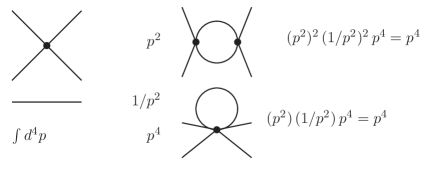
Figure 1: Illustration of power counting in ChPT. On the left are shown: The lowest order vertex, the meson propagator, a loop momentum integration and their respective powers of a generic momentum $p$. The examples on the right show two one-loop diagrams that count as $\mathcal{O}(p^{4})$ as compared to $\mathcal{O}(p^{2})$ for the lowest order.

In order to perform the power counting expansion, higher order Lagrangians need to be constructed. This has to be done in order to know the total number of parameters needed at a given order in the expansion. These parameters are referred to as low-energy constants (LECs). This classification was done at $\mathcal{O}(p^{4})$ by Gasser and Leutwyler [3, 4] and at $\mathcal{O}(p^{6})$ in Ref. [7]. The number of LECs needed for the partially quenched case was determined in Ref. [8, 9]. A summary of these results is given in Table 1.

Table 1: The number of LECs (physical + contact terms) at the various orders in mesonic ChPT.

	2 flavour		3 flavour		3+3 PQ
$\mathcal{O}(p^{2})$	$F,B$	2	$F_{0},B_{0}$	2	$F_{0},B_{0}$	2
$\mathcal{O}(p^{4})$	$l_{i}^{r},h_{i}^{r}$	7+3	$L_{i}^{r},H_{i}^{r}$	10+2	$\hat{L}_{i}^{r},\hat{H}_{i}^{r}$	11+2
$\mathcal{O}(p^{6})$	$c_{i}^{r}$	53+4	$C_{i}^{r}$	90+4	$K_{i}^{r}$	112+3

The main problem here is to determine a minimal set of LECs. No simple and straightforward procedure is known for the determination of such a set. Only if all of the LECs can be separately determined from “experiment”, or more generally from QCD Green’s functions, can one be sure that the set of LECs is indeed minimal. Heat kernel methods allow to determine the divergence structure independently of Feynman diagram calculations. This, done at $\mathcal{O}(p^{4})$ in [3, 4] and at $\mathcal{O}(p^{6})$ in [10], provides a very welcome check on actual two-loop calculations.

3 Partially Quenched QCD

One of the major applications of ChPT at present, and likely even more so in the future, is the extrapolation of lattice QCD results to the physical values of the light $u,d$ quark masses. An overview of the many uses of ChPT in lattice QCD can be found in the recent lectures by Sharpe [11]. The main emphasis here is on the partially quenched aspect, which can be implemented in lattice gauge theory. In order to extract observables, one typically evaluates a correlator, e.g. a two-point correlator to obtain masses and decay constants. This correlator is evaluated in Euclidean space via the path integral (or functional integral) formalism:

$$\langle 0|(\overline{u}\gamma_{5}d)(x)(\overline{d}\gamma_{5}u)(0)|0\rangle = \displaystyle\int[dq][d\overline{q}][dG]\>(\overline{u}\gamma_{5}d)(x)(\overline{d}\gamma_{5}u)(0)$$ (3)

$$\times \exp\left[{\displaystyle i\int d^{4}y\>\mathcal{L}_{\mathrm{QCD}}}\right],$$

where the integral over the quarks and the anti-quarks can be performed and one obtains, schematically,

$$\displaystyle\int[dq][d\overline{q}][dG]\>(\overline{u}\gamma_{5}d)(x)(\overline{d}\gamma_{5}u)(0)\>\exp\left[{\displaystyle i\int d^{4}y\>\mathcal{L}_{\mathrm{QCD}}}\right]\>\propto$$ (4)

$$\int[dG]\>\underbrace{\exp\left[-i\int d^{4}x\>\frac{G_{\mu\nu}G^{\mu\nu}}{4}\right]}_{\mbox{gluonic}}\>\overbrace{(D\hskip-6.00006pt/\,^{u}_{G})^{-1}(x,0)(D\hskip-6.00006pt/\,^{d}_{G})^{-1}(0,x)}^{\mbox{valence}}\>\underbrace{\det\left(D\hskip-6.00006pt/\,_{G}\right)_{\mathrm{QCD}}}_{\mbox{sea}},$$

where $D\hskip-6.00006pt/\,_{G}$ denotes the full Dirac operator with a specific gluon field configuration but including the quark masses. The remaining integral over all the gluon degrees of freedom in Eq. (4) is performed by importance sampling. The part labeled “valence” is connected to the external sources (hence the name), while the part labeled “sea” describes the effects of closed quark loops, not connected to any outside lines. Of course, gluons provide couplings between all these fermion lines if we look at the functional integral as a sum over Feynman diagrams.

One major problem is that the determinant labeled “sea” is extremely CPU time consuming to evaluate. This has led to several approximations, the most drastic of which is the quenched approximation, whereby the sea contribution is completely neglected and only the gluonic and valence ones retained. “Unquenched” means in this respect that the sea determinant is included. However, the high CPU time requirements make it difficult to vary the quark masses very much in this part, and changing quark masses in the part labelled “valence” is indeed computationally much cheaper. In partially quenched simulations one thus varies the sea and valence quark masses independently of each other. There are good arguments in favour of this approach:

• It is clearly superior to the quenched approximation.

• More systematic studies of the input parameters may be performed.

• It turns out that some quantities can be extracted from different observables in this way.

• Unlike the quenched approximation, it is continuously connected to the QCD case.

However, a number of drawbacks need to be remembered:

• It is not QCD as soon as quark masses are different in the valence and sea sectors.

• It is not a bona fide Quantum Field Theory so the spin-statistics theorem and unitarity relations are not satisfied.

Especially the latter point might be important, since the derivation of ChPT from QCD relies heavily on unitarity. Nonetheless, one expects that at least close to the QCD case, PQQCD will have a low-energy effective theory similar to ChPT.

4 Partially Quenched ChPT at Two Loops

The central problem in PQChPT is thus to mimic, within ChPT, the effect of treating closed quark loops and quark lines differently. This problem is depicted schematically in Fig. 2. In some of the early calculations, the quark flow was inferred directly from the flavour flow in the ChPT vertices. An alternative approach, often referred to as the supersymmetric method, is more systematic. A series of bosonic ghost quarks with spin 1/2 is added to QCD. Due to the different statistics, these may cancel the effects of closed loops of valence quarks. This method is illustrated in Fig. 3.

Figure 2: The meson loop diagram on the left has different types of quark flow, both valence and sea quark as indicated on the right.

Figure 3: The effect of adding ghost quarks to the different quark loops in the mesonic one loop diagram shown on the right.

The supersymmetric method was originally introduced for the quenched case in Refs. [12, 13, 14] and later extended to the partially quenched case, see Refs. [15, 16, 17] and references therein. Also, an instructive discussion about ChPT in the partially quenched sector is given in Ref. [16]. For practical purposes, the QCD chiral symmetry may be replaced by a graded symmetry which is (assumed to be) spontaneously broken to its diagonal subgroup:

$$SU(n_{v}+n_{s}|n_{v})_{L}\times SU(n_{v}+n_{s}|n_{v})_{R}\to SU(n_{v}+n_{s}|n_{v})_{V},$$ (5)

where $n_{v},n_{s}$ denote the number of valence and sea quark flavours. The “Goldstone bosons” now have both fermionic and bosonic character. A large amount of work exists at one-loop order, see the references in [11]. One stumbling block at two-loop order was the determination of the divergence structure and Lagrangians. Fortunately, it was realized [8, 18, 19, 9] that the work of [7, 10] could be taken over by formally replacing traces by supertraces and the general number of flavours by the number of sea quarks.

The final expressions at two-loop order are highly complex, which is due in part to the larger number of independent quark masses, but mainly to the peculiarities of the flavour neutral mesons. These do not have a simple pole structure but consist instead of several terms including a double pole:

$$\!\!-i\,G_{ij}^{n}(k)=\frac{\epsilon_{j}}{k^{2}\!-\!\chi_{ij}}-\frac{1}{n_{\mathrm{sea}}}\left[\frac{R^{d}_{i}}{(k^{2}\!-\!\chi_{i})^{2}}+\frac{R^{c}_{i}}{k^{2}\!-\!\chi_{i}}+\frac{R_{\eta ii}^{\pi}}{k^{2}\!-\!\chi_{\pi}}+\frac{R_{\pi ii}^{\eta}}{k^{2}\!-\!\chi_{\eta}}\right],$$ (6)

where the various $R$ coefficients consist of powers of ratios of differences of quark masses [13, 16]. The presence of the many ratios leads to the extremely long expressions. The double pole in Eq. (6) is due to the fact that PQChPT is not a full field theory. Thus the valence quark loops cannot be resummed to all orders, as shown in Fig. 4.

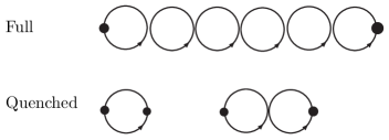
Figure 4: Schematic resummation of quark loops. Imagine gluons everywhere on top of the quark lines drawn. Each bubble gives a lowest order meson propagator. The full resummation exponentiates and leads to a single pole. For valence quarks only the loops shown at the bottom appear, leading to double poles in the propagator.

A large amount of work exists in PQChPT at two loops. The first calculation was the meson mass for the case of three sea quarks, with a common valence mass and a common sea quark mass [8]. Since then the decay constants [18] and masses [9] have been fully worked out. These quantities are also fully known for two sea quark flavours [19]. The formulas are rather lengthy and the number of parameters is also quite high. Analytical programs have therefore been posted by the authors on the website [6]. Methods of dealing with the large number of parameters have been discussed extensively in Refs. [19] and [9] for the two- and three-flavour cases, respectively. It should be emphasized again that the LECs of unquenched ChPT, and thus the full QCD results, are related to the partially quenched LECs in a simple way via the Cayley-Hamilton relations of Ref. [7]. More recent work has focused on the neutral mass sector of PQChPT. It was shown in Ref. [16] how the residue ${\cal D}$ of the double pole

$$G^{n}_{ij}(k)=\frac{-i{\cal Z}{\cal D}}{(k^{2}-M^{2}_{ch})^{2}}\>+\>\cdots$$ (7)

can be measured on the lattice and used at $\mathcal{O}(p^{4})$ to extract $L_{7}^{r}$, which is relevant for the $\eta$ mass. In Ref. [20] the self-energy resummation was worked out to all orders, and it was shown explicitly how to obtain the double pole and the structure of the full propagator from the one-particle irreducible diagrams. It was also shown that all $\mathcal{O}(p^{6})$ parameters relevant for the $\eta$ mass can be extracted using this method. The most recent work has focused on the inclusion of dynamical photons in the partially quenched theory [21].

5 Standard ChPT at Two Loops

The existing work at two-loop order in mesonic ChPT is very briefly reviewed here. A much more extensive review may be found in Ref. [1]. The oldest two-loop work in ChPT made use of dispersive techniques to calculate the non-analytical dependence on the kinematical variables. This was done numerically [22] and analytically [23] for the pion vector and scalar form factors, and fully analytically for $\pi\pi$ scattering in Ref. [24]. The first full two-loop calculations appeared somewhat later in the two-flavour sector, with $\gamma\gamma\to\pi^{0}\pi^{0}$ [25] and $\gamma\gamma\to\pi^{+}\pi^{-}$, $F_{\pi}$ and $m_{\pi}$ [26]. The process $\gamma\gamma\to\pi\pi$ was recently recalculated in Ref. [27]. With $\pi\pi$ scattering [28], pion vector and scalar form factors [29] and the radiative decay of the pion [30], most processes of interest have now been worked out.

The earliest three-flavour work, on the vector two-point functions, was by Golowich and Kambor [31], extended to all flavour cases in Refs. [32, 33, 34]. The first calculations with proper two-loop integrals were of the meson masses and decay constants, in Refs. [35, 33] and [36], including isospin violation. All scalar two point functions [37, 38] and vacuum expectation values [39] are also known. More recent work covers the electromagnetic form factors [40, 41], $K_{\ell 3}$ [40, 42], and scalar form-factors [43]. Processes with more external legs include $K_{ell4}$ [39], kaon radiative decay [44], $\pi\pi$ [45] and $\pi K$ [46] scattering. The first results at finite volume have appeared recently [47, 48].

A major problem in phenomenological applications of ChPT at two loops is to find enough experimental inputs to determine the $\mathcal{O}(p^{6})$ parameters. In practice most of them have to be estimated, which is typically done along the lines of Ref. [49] by saturating the LECs by resonance exchange. While this can be done at various levels of sophistication, most phenomenological applications have used a fairly simple extension of Ref. [49], see e.g. Refs. [28, 39, 36, 41, 42, 45, 46].

Most phenomenological applications rely on the work of Refs. [39, 36]. The fitting method and the inputs used are described in detail in Ref. [36], and the results can be found in Table 2, in the columns labeled “fit 10”. These used the (at that time) most recent data of the BNL E865 experiment as the main $K_{\ell 4}$ input. The change compared to a fit at $\mathcal{O}(p^{4})$ is also given in Table 2. These fits assume that the $1/N_{c}$ suppressed LECs $L_{4}^{r}$ and $L_{6}^{r}$ vanish at the scale $\mu=0.77$ GeV. On the other hand, “Fit D” of Ref. [46] uses all the same inputs as “fit 10”, in addition to the dispersive results on $\pi\pi$ and $\pi K$ scattering from Refs. [50] and [51]. The convergence properties of some quantities are also given in Table 2. However, an update of the fit is in order, with the new experimental results on $K_{\ell 4}$ and an improved treatment of the $\mathcal{O}(p^{6})$ constants along the lines of Ref.[52, 53].

Table 2: The fitted optimal values of the $L_{i}^{r}$ at $\mathcal{O}(p^{4})$ and $\mathcal{O}(p^{6})$, and convergence behviour of several quantities for the different fits [36, 46].

	fit 10, $\mathcal{O}(p^{6})$	fit 10, $\mathcal{O}(p^{4})$	fit D
$10^{3}L_{1}^{r}$	$0.43\pm 0.12$	$0.38$	$0.44$
$10^{3}L_{2}^{r}$	$0.73\pm 0.12$	$1.59$	$0.69$
$10^{3}L_{3}^{r}$	$-2.53\pm 0.37$	$-2.91$	$-2.33$
$10^{3}L_{4}^{r}$	$\equiv 0$	$\equiv 0$	$\equiv 0.2$
$10^{3}L_{5}^{r}$	$0.97\pm 0.11$	$1.46$	$0.88$
$10^{3}L_{6}^{r}$	$\equiv 0$	$\equiv 0$	$\equiv 0$
$10^{3}L_{7}^{r}$	$-0.31\pm 0.14$	$-0.49$	$-0.28$
$10^{3}L_{8}^{r}$	$0.60\pm 0.18$	$1.00$	$0.54$
$2B_{0}\hat{m}/m_{\pi}^{2}$	0.736	0.991	0.958
$m_{\pi}^{2}$: $\mathcal{O}(p^{4})$, $\mathcal{O}(p^{6})$	0.006, 0.258	0.009, $\equiv 0$	$-$0.091, 0.133
$m_{K}^{2}$: $\mathcal{O}(p^{4})$, $\mathcal{O}(p^{6})$	0.007, 0.306	0.075, $\equiv 0$	$-$0.096, 0.201
$m_{\eta}^{2}$: $\mathcal{O}(p^{4})$, $\mathcal{O}(p^{6})$	$-$0.052, 0.318	0.013, $\equiv 0$	$-$0.151, 0.197
$m_{u}/m_{d}$	$0.45\pm 0.05$	0.52	0.50
$F_{0}$ [MeV]	87.7	81.1	80.4
$\frac{F_{K}}{F_{\pi}}$: $\mathcal{O}(p^{4})$, $\mathcal{O}(p^{6})$	0.169, 0.051	0.22, $\equiv 0$	0.159, 0.061

6 Conclusions

ChPT at two-loop order is by now a very well developed field, where a large number of two- and three-flavour calculations have been performed. The use of the partially quenched results will hopefully allow for many of the $\mathcal{O}(p^{6})$ LECs to be determined from Lattice QCD, thus removing a major stumbling block in phenomenological applications.

References

- [1] J. Bijnens, hep-ph/0604043, to be published in Prog. Part. Nucl. Phys.
- [2] S. Weinberg, Physica A 96 (1979) 327.
- [3] J. Gasser and H. Leutwyler, Ann. Phys. 158 (1984) 142.
- [4] J. Gasser and H. Leutwyler, Nucl. Phys. B250 (1985) 465.
- [5] S. Scherer, hep-ph/0210398; G. Ecker, hep-ph/0011026; A. Pich, hep-ph/9806303.
- [6] The website http://www.thep.lu.se/bijnens/chpt.html contains many of the analytical formulas as well as a list of lectures on ChPT.
- [7] J. Bijnens et al., JHEP 9902 (1999) 020 [hep-ph/9902437].
- [8] J. Bijnens et al., Phys. Rev. D70(2004)111503 [hep-lat/0406017].
- [9] J. Bijnens et al., Phys. Rev. D73 (2006) 074509 [hep-lat/0602003].
- [10] J. Bijnens et al., Ann. Phys. 280 (2000) 100 [hep-ph/9907333].
- [11] S. Sharpe, hep-lat/0607016.
- [12] A. Morel, J. Phys. (France) 48 (1987) 1111.
- [13] C. Bernard and M. Golterman, Phys. Rev. D46 (1992) 853 [hep-lat/9204007].
- [14] S. Sharpe, Phys. Rev. D46 (1992) 3146 [hep-lat/9205020].
- [15] C. Bernard and M. Golterman, Phys. Rev. D49 (1994) 486 [hep-lat/9306005].
- [16] S. Sharpe and N. Shoresh, Phys. Rev. D62 (2000) 094503 [hep-lat/0006017].
- [17] S. Sharpe and N. Shoresh, Phys. Rev. D64 (2001) 114510 [hep-lat/0108003].
- [18] J. Bijnens and T. Lähde, Phys. Rev. D71 (2005) 094502 [hep-lat/0501014].
- [19] J. Bijnens and T. Lähde, Phys. Rev. D72 (2005) 074502 [hep-lat/0506004].
- [20] J. Bijnens and N. Danielsson, Phys. Rev. D74 (2006) 054503 [hep-lat/0606017].
- [21] J. Bijnens and N. Danielsson, Phys. Rev. D75 (2007) 014505 [hep-lat/0610127].
- [22] J. Gasser and Ulf-G. Meißner, Nucl. Phys. B 357 (1991) 90.
- [23] G. Colangelo et al., Phys. Rev. D 54 (1996) 4403 [hep-ph/9604279].
- [24] M. Knecht et al., Nucl. Phys. B 457 (1995) 513 [hep-ph/9507319].
- [25] S. Bellucci et al., Nucl. Phys. B423 (1994) 80 [Erratum-ibid. B431 (1994) 413] [hep-ph/9401206].
- [26] U. Bürgi, Phys. Lett. B377 (1996) 147 [hep-ph/9602421]; Nucl. Phys. B479 (1996) 392 [hep-ph/9602429].
- [27] J. Gasser et al., Nucl. Phys. B 728 (2005) 31 [hep-ph/0506265]; Nucl. Phys. B745 (2006) 84 [hep-ph/0602234].
- [28] J. Bijnens et al., Phys. Lett. B 374 (1996) 210 [hep-ph/9511397]; Nucl. Phys. B 508 (1997) 263 [Erratum-ibid. B 517 (1998) 639] [hep-ph/9707291].
- [29] J. Bijnens et al., JHEP 9805 (1998) 014 [hep-ph/9805389].
- [30] J. Bijnens and P. Talavera, Nucl. Phys. B 489, 387 (1997) [hep-ph/9610269].
- [31] E. Golowich and J. Kambor, Nucl. Phys. B 447, 373 (1995) [hep-ph/9501318].
- [32] S. Dürr and J. Kambor, Phys. Rev. D61 (2000) 114025 [hep-ph/9907539].
- [33] G. Amorós et al., Nucl. Phys. B568 (2000) 319 [hep-ph/9907264].
- [34] K. Maltman, Phys. Rev. D 53 (1996) 2573 [hep-ph/9504404]; K. Maltman and C. E. Wolfe, Phys. Rev. D 59 (1999) 096003 [hep-ph/9810441].
- [35] E. Golowich and J. Kambor, Phys. Rev. D 58, 036004 (1998) [hep-ph/9710214].
- [36] G. Amorós et al., Nucl. Phys. B 602 (2001) 87 [hep-ph/0101127].
- [37] B. Moussallam, JHEP 0008 (2000) 005 [hep-ph/0005245].
- [38] J. Bijnens, unpublished.
- [39] G. Amorós et al., Phys. Lett. B480 (2000) 71 [hep-ph/9912398]; Nucl. Phys. B585 (2000) 293 [Erratum-ibid. B598 (2001) 665] [hep-ph/0003258].
- [40] P. Post and K. Schilcher, Phys. Rev. Lett. 79(1997)4088[hep-ph/9701422]; Nucl. Phys. B599(2001)30[hep-ph/0007095]; Eur. Phys. J. C25(2002)427[hep-ph/0112352].
- [41] J. Bijnens and P. Talavera, JHEP 0203 (2002) 046 [hep-ph/0203049].
- [42] J. Bijnens and P. Talavera, Nucl. Phys. B669 (2003) 341 [hep-ph/0303103].
- [43] J. Bijnens and P. Dhonte, JHEP 0310 (2003) 061 [hep-ph/0307044].
- [44] C. Geng et al., Nucl. Phys. B 684 (2004) 281 [hep-ph/0306165].
- [45] J. Bijnens et al., JHEP 0401 (2004) 050 [hep-ph/0401039].
- [46] J. Bijnens et al., JHEP 0405 (2004) 036 [hep-ph/0404150].
- [47] J. Bijnens and K. Ghorbani, Phys. Lett. B636, 51 (2006) [hep-lat/0602019].
- [48] G. Colangelo, S. Dürr and C. Haefeli, Nucl. Phys. B721, 136 (2005) [hep-lat/0503014].
- [49] G. Ecker, J. Gasser, A. Pich and E. de Rafael, Nucl. Phys. B321 (1989) 311.
- [50] G. Colangelo, J. Gasser and H. Leutwyler, Nucl. Phys. B603 (2001) 125 [hep-ph/0103088].
- [51] P. Büttiker, S. Descotes-Genon and B. Moussallam, Eur. Phys. J. C 33 (2004) 409 [hep-ph/0310283].
- [52] J. Bijnens, E. Gámiz, E. Lipartia and J. Prades, JHEP 0304 (2003) 055 [hep-ph/0304222].
- [53] V. Cirigliano, G. Ecker, M. Eidemuller, R. Kaiser, A. Pich and J. Portoles, Nucl. Phys. B753 (2006) 139 [hep-ph/0603205].