Heavy-to-light form factors on the light cone

Abstract

The light cone method provides a convenient non-perturbative tool to study the heavy-to-light form factors. We construct a light cone quark model utilizing the soft collinear effective theory. In the leading order of effective theory, the form factors for $B$ to light pseudoscalar and vector mesons are reduced to three universal form factors which can be calculated as overlaps of hadron light cone wave functions. The numerical results show that the leading contribution is close to the results from other approaches. The $q^{2}$ dependence of the heavy-to-light form factors are also presented.

I Introduction

The hadronic matrix elements of weak $B$ decays to a light pseudoscalar (P) and to a vector meson (V) are described by $B\to P$ and $B\to V$ transition form factors, respectively. These heavy-to-light form factors are essential to study the semileptonic and even non-leptonic $B$ decays. Information on the form factors is crucial to test the mechanism of CP violation in the Standard Model and to extract the CKM parameters CKM . For instance, the $B\to\pi(\rho)$ form factors are required to determine the CKM matrix element $|V_{ub}|$ precisely. In $B\to V\gamma$ and $B\to Vl^{+}l^{-}$ processes which are sensitive to new physics, the precise evaluation of $B\to V$ form factors is indispensable. Another interesting reason for the study of the heavy-to-light form factors is that they provide an ideal laboratory to explore the rich structures of QCD dynamics. At the large recoil region where the final state light meson moves fast, the heavy-to-light system contains internal information on both short and long distance QCD dynamics with the factorization theorem.

There are already many methods calculating the heavy-to-light transition form factors in the literature such as simple quark model bsw , the light cone quark models (LCQM) Jaus1 ; CCH1 ; CJK ; CCH2 , the light cone sum rules (LCSR) LCSRP ; BZpseudo ; BZvector , the perturbative QCD (PQCD) approach based on $k_{T}$ factorization PQCD etc.

In Ref. CYOPR , a model-independent way to look for relations between different form factors is suggested by analogy with the heavy-to-heavy transitions IW . One important observation is that in the heavy quark mass and large energy of light meson limit, the spin symmetry relates the form factors for $B\to P$ and $B\to V$ to three universal energy-dependent functions: $\zeta_{P}$ for pseudoscalar meson; and $\zeta_{||},~{}\zeta_{\bot}$ for longitudinally and transversely polarized vector meson, respectively. The development of soft collinear effective theory (SCET) makes the analysis on a more rigorous foundation. The SCET is a powerful method to systematically separate the dynamics at different scales: hard scale $m_{b}$ ($b$ quark mass), hard intermediate scale $\mu_{hc}=\sqrt{m_{b}\Lambda_{\rm QCD}}$, soft scale $\Lambda_{\rm QCD}$ and to sum large logs using the renormalization group technics. After a series of researches SCETff1 ; SCETff2 ; BCDF ; SCETff3 ; SCETff4 , a factorization formula is established for the heavy-to-light form factors in the heavy quark mass and large energy limit as

$$F_{i}(q^{2})=C_{i}(E,\mu_{I})\zeta_{j}(\mu_{I},E)+\phi_{B}(\omega,\mu_{II})\otimes T_{i}(E,u,\omega,\mu_{II})\otimes\phi_{M}(u,\mu_{II}),$$ (1)

where the indices $j$ represent ${(P,||,\bot)}$ and $\otimes$ denotes the convolutions over light cone momentum factions. $\phi_{B}(\omega)$ and $\phi_{M}(u)$ are light cone distribution amplitudes for $\bar{B}$ and light mesons. The coefficients $C_{i}$ and $T_{i}$ are perturbatively calculable functions which include hard gluon corrections. The functions $\zeta_{j}$ denote the universal functions that satisfies the spin symmetry.

Although soft collinear effective theory is really powerful and rigorous, the form factors $\zeta_{j}$ cannot be directly calculated. These functions are non-perturbative in principle and the evaluation of them relies on non-perturbative methods. Lattice simulation on heavy-to-light form factors is usually restricted to the region with final meson energy $E<1\mbox{ GeV}$ and cannot be applied to our case directly where the light meson carries the energy of order $M_{B}/2$. The construction of LCSR within SCET has been explored recently in SCETLCSR1 ; SCETLCSR2 ; SCETLCSR3 . In these studies, only the pseudoscalar meson form factor $\zeta_{P}$ are calculated at present.

The light cone field theory provides another natural language to study these processes. As pointed out in BPP , light cone QCD has some unique features which are particularly suitable to describe a hadronic bound state. For instance, the vacuum state in this approach is much simpler than that in other approaches. The light cone wave functions, which describe the hadron in terms of their fundamental quark and gluon degrees of freedom, are independent of the hadron momentum and thus are explicitly Lorentz invariant. The light cone Fock space expansion provides a complete relativistic many-particle basis for a hadron. For hard exclusive processes with large momentum transfer, factorization theorem in the perturbative light cone QCD makes first-principle predictions LB . For non-perturbative QCD, an approach which combines the advantage of light cone method with the low energy constituent quark model is more appealing. This approach, which we will call light cone quark model (LCQM), has been successfully applied to the calculation of the meson decay constants and hadronic form factors Jaus1 ; Jaus2 ; CCH1 ; CJK ; CCH2 ; LFHW .

As far as the form factors are concerned, they can be generally represented by the convolution of $B$ and light meson wave functions in the light cone approach as

$$F(q^{2})=\sum\limits_{n_{1},n_{2}}\int\left\{\overline{\prod\limits_{i}}\frac{dx_{i}d^{2}k_{\bot i}}{16\pi^{3}}\right\}\left\{\overline{\prod\limits_{j}}\frac{dx_{j}d^{2}k_{\bot j}}{16\pi^{3}}\right\}\Psi_{M}^{(n_{1})*}(x_{i},k_{\bot i})\Psi_{B}^{(n_{2})}(x_{j},k_{\bot j}).$$ (2)

where the sum is over all Fock states with $n_{1},~{}n_{2}$ the particle numbers, $i,j$ denote the $i$- and $j$-th constitutes of the light meson and $\bar{B}$ meson, respectively. The product is performed over the longitudinal momentum fractions $x_{i,j}$ and the transverse momenta $k_{\bot i,j}$. The light cone wave function $\Psi(x,k_{\bot})$ is the generalization of distribution amplitude $\phi(x)$ by including the transverse momentum distributions. This formulation contains both hard and soft interactions.

The main purpose of this paper is to develop a non-perturbative light cone approach within the soft collinear effective theory and to evaluate the three universal heavy-to-light form factors directly. The close relation between the light cone QCD and soft collinear effective theory was noted in BCDF . The SCET has the advantage that a systematic power expansion with small parameter $\Lambda_{\rm QCD}/m_{b}$ (or $\sqrt{\Lambda_{\rm QCD}/m_{b}}$) can be performed to improve the calculation accuracy order by order. The combination of the two methods can reduce the model dependence of non-perturbative methods. In the conventional light cone approach, all the quarks are on-shell. Now in the new approach, it is convenient to choose the light energetic quark as the collinear mode in the soft collinear effective theory and the heavy quark field as that in the heavy quark effective theory. The spectator antiquark is remained as the soft mode. By this way, the light cone quark model within the soft collinear effective theory is established. Then we can calculate the $B\to P$ and $B\to V$ form factors order by order.

The paper is organized as follows. In Section II, we first present the definition of the three universal form factors from the spin symmetry relations. We then discuss a light cone quark model within soft collinear effective theory. The numerical results for the form factors and discussions are presented in Section III. The final part contains our conclusion.

II The heavy-to-light form factors in the light cone approach

II.1 Definitions of the heavy-to-light form factors

The $\bar{B}\to P$ and $\bar{B}\to V$ form factors are defined under the conventional form as follows

$$\langle P(P^{\prime})|\bar{q}\gamma^{\mu}b|\bar{B}(P)\rangle = f_{+}(q^{2})\left[(P+P^{\prime})^{\mu}-\frac{M_{B}^{2}-M_{P}^{2}}{q^{2}}q^{\mu}\right]+f_{0}(q^{2})\frac{M_{B}^{2}-M_{P}^{2}}{q^{2}}q^{\mu},$$

$$\langle P(P^{\prime})|\bar{q}\sigma^{\mu\nu}q_{\nu}b|\bar{B}(P)\rangle = i\frac{f_{T}(q^{2})}{M_{B}+M_{P})}\left[q^{2}(P+P^{\prime})^{\mu}-(M_{B}^{2}-M_{P}^{2})q^{\mu}\right],$$

$$\langle V(P^{\prime},\epsilon^{*})|\bar{q}\gamma^{\mu}b|\bar{B}(P)\rangle = -\frac{2V(q^{2})}{M_{B}+M_{V}}\epsilon^{\mu\nu\rho\sigma}\epsilon^{*}_{\nu}P_{\rho}P^{\prime}_{\sigma},$$

$$\langle V(P^{\prime},\epsilon^{*})|\bar{q}\gamma^{\mu}\gamma_{5}b|\bar{B}(P)\rangle = 2iM_{V}A_{0}(q^{2})\frac{\epsilon^{*}\cdot q}{q^{2}}q^{\mu}+i(M_{B}+M_{V})A_{1}(q^{2})\left[\epsilon^{*}_{\mu}-\frac{\epsilon^{*}\cdot q}{q^{2}}q^{\mu}\right]$$

$$-iA_{2}(q^{2})\frac{\epsilon^{*}\cdot q}{M_{B}+M_{V}}\left[(P+P^{\prime})^{\mu}-\frac{M_{B}^{2}-M_{V}^{2}}{q^{2}}q^{\mu}\right],$$

$$\langle V(P^{\prime},\epsilon^{*})|\bar{q}\sigma^{\mu\nu}q_{\nu}b|\bar{B}(P)\rangle = -2iT_{1}(q^{2})\epsilon^{\mu\nu\rho\sigma}\epsilon^{*}_{\nu}P_{\rho}P^{\prime}_{\sigma},$$

$$\langle V(P^{\prime},\epsilon^{*})|\bar{q}\sigma^{\mu\nu}\gamma_{5}q_{\nu}b|\bar{B}(P)\rangle = iT_{2}(q^{2})\left[(M_{B}^{2}-M_{V}^{2})\epsilon^{*\mu}-(\epsilon^{*}\cdot q)(P+P^{\prime})^{\mu}\right]$$ (3)

$$+iT_{3}(q^{2})(\epsilon^{*}\cdot q)\left[q^{\mu}-\frac{q^{2}}{M_{B}^{2}-M_{V}^{2}}(P+P^{\prime})^{\mu}\right],$$

where $q=P-P^{\prime}$ is the momentum transfer, $M_{B}$ the $\bar{B}$ meson mass, $M_{P,V}$ the mass of the pseudoscalar and vector mesons, $\epsilon$ the polarization vector of the vector meson. We have used the convention $\epsilon^{0123}=+1$. In the following, we choose the convention within which the vectors $n_{\pm}$ are $n_{+}^{\mu}=(1,0,0,-1)$, $n_{-}^{\mu}=(1,0,0,1)$ and the light cone momentum components are $p^{+}=n_{+}\cdot p=p^{0}+p^{3}$, $p^{-}=n_{-}\cdot p=p^{0}-p^{3}$, $p_{b}=m_{b}v$. Our convention for the vectors $n_{\pm}$ are different from that in most literatures. In the above definitions, there are ten form factors in total: $f_{+}$, $f_{0}$, $f_{T}$ for the pseudoscalar meson; $V,~{}A_{0},~{}A_{1},~{}A_{2},~{},T_{1},~{}T_{2},~{}T_{3}$ for the vector meson. Note that the form factors are in general different for each hadron.

In SCET, the energetic light quark is described by its leading two component spinor $\xi=\frac{\hbox to0.0pt{\hskip 0.28436pt/\hss}{n}_{-}\hbox to0.0pt{\hskip 0.28436pt/\hss}{n}_{+}}{4}q$ and the heavy quark is replaced by $h_{v}=e^{im_{b}v\cdot x}\frac{(1+\hbox to0.0pt{/\hss}{v})}{2}b$. The weak current $\bar{q}\Gamma b$ in full QCD is matched onto the SCET current $\bar{\xi}\Gamma h_{v}$ at tree level where we have omitted the Wilson lines for simplicity. For an arbitrary matrix $\Gamma$, $\bar{\xi}\Gamma h_{v}$ has only three independent Dirac structures. One convenient choice is discussed in Ref. SCETff1 ; relation : $\bar{\xi}h_{v}$, $\bar{\xi}\gamma_{5}h_{v}$ and $\bar{\xi}\gamma_{\bot}^{\mu}h_{v}$. It can be seen from a trace technology by

$$\frac{\hbox to0.0pt{\hskip 0.28436pt/\hss}{n}_{+}\hbox to0.0pt{\hskip 0.28436pt/\hss}{n}_{-}}{4}\Gamma\frac{(1+\hbox to0.0pt{/\hss}{v})}{2}=\frac{\hbox to0.0pt{\hskip 0.28436pt/\hss}{n}_{+}\hbox to0.0pt{\hskip 0.28436pt/\hss}{n}_{-}}{4}\left[c_{1}+c_{2}\gamma_{5}+c_{3}\gamma_{\bot}^{\mu}\right]\frac{(1+\hbox to0.0pt{/\hss}{v})}{2},$$ (4)

where $c_{i}$s are defined as:

$$c_{1}=\frac{1}{4}{\rm Tr}\left[(1+\hbox to0.0pt{/\hss}{v})\hbox to0.0pt{\hskip 0.28436pt/\hss}{n}_{-}\Gamma\right],\qquad\qquad c_{2}=\frac{1}{4}{\rm Tr}\left[(1+\hbox to0.0pt{/\hss}{v})\hbox to0.0pt{\hskip 0.28436pt/\hss}{n}_{-}\gamma_{5}\Gamma\right],$$

$$c_{3}=\frac{1}{4}{\rm Tr}\left[(1+\hbox to0.0pt{/\hss}{v})\hbox to0.0pt{\hskip 0.28436pt/\hss}{n}_{-}\gamma_{\bot\mu}\Gamma\right].$$ (5)

The above spin symmetry leads to non-trivial relations for the heavy-to-light form factors: the ten form factors are reduced to three independent universal form factors. The $B$ to light universal form factors $\zeta_{P}$, $\zeta_{||,\perp}$ are defined as

$$\langle P|\bar{\xi}h_{v}|\bar{B}\rangle = 2E\zeta_{P}(E),$$

$$\langle V|\bar{\xi}\gamma_{5}h_{v}|\bar{B}\rangle = -2iM_{V}\zeta_{||}(E)v\cdot\epsilon^{*},$$

$$\langle V|\xi\gamma^{\mu}_{\perp}h_{v}|\bar{B}\rangle = -2E\zeta_{\perp}(E)\epsilon^{\mu\nu\rho\sigma}\epsilon_{\nu}^{*}v_{\rho}n_{-\sigma},$$ (6)

where $E=(M_{B}^{2}-q^{2})/2M_{B}$ is the energy of the light meson (neglecting the small mass of the final state meson) and $q$ is the momentum transfer. $\zeta_{i(i=P,||,\zeta)}$ are functions of energy of the light meson. Up to leading order of $\alpha_{s}$ and leading power of $\Lambda_{\rm QCD}/m_{b}$, the total ten physical form factors are determined from the three independent factors to the leading order of $\alpha_{s}$ as

$$f_{+}(q^{2})=\frac{M_{B}}{2E}f_{0}(q^{2})=\frac{M_{B}}{M_{B}+M_{P}}f_{T}(q^{2})=\zeta_{P}(E),$$

$$\frac{M_{B}}{M_{B}+M_{V}}V(q^{2})=\frac{M_{B}+M_{V}}{2E}A_{1}(q^{2})=\zeta_{\bot}(E),$$

$$A_{0}(q^{2})=\zeta_{||}(E),\qquad A_{2}(q^{2})=\frac{M_{B}}{M_{B}-M_{V}}\left[\zeta_{\bot}(E)-\frac{M_{V}}{E}\zeta_{||}(E)\right],$$

$$T_{1}(q^{2})=\frac{M_{B}}{2E}T_{2}(q^{2})=\zeta_{\bot}(E),\qquad T_{3}(q^{2})=\zeta_{\bot}(E)-\frac{M_{V}}{E}\zeta_{||}(E).$$ (7)

As in CYOPR ; BF1 , we keep the leading kinematic light meson mass correction and neglect the higher $M_{P,V}^{2}/M_{B}^{2}$ terms.

II.2 Light cone quark model

We start with a discussion of hadron bound states on the light cone. The goal is to find a relativistic invariant description of the hadron in terms of its fundamental quark and gluon constitutes. For a complete Fock state basis $|n\rangle$, the hadron is expanded by a series of wave functions: $|h\rangle=\sum\limits_{n}|n\rangle\langle n|h\rangle=\sum\limits_{n}|n\rangle\psi_{n/h}$. It is convenient to use a light cone Fock state basis on which the hadron with momentum $\tilde{P}=(P^{+},P_{\bot})$ is described by BPP

$$|h:\tilde{P}\rangle=\sum\limits_{n,\lambda_{i}}\int\left\{\overline{\prod\limits_{i}}\frac{dx_{i}d^{2}k_{\bot i}}{\sqrt{x_{i}}16\pi^{3}}\right\}|n:x_{i}P^{+},x_{i}P_{\bot i}+k_{\bot i},\lambda_{i}\rangle\Psi_{n/h}(x_{i},k_{\bot i},\lambda_{i}),$$ (8)

where the sum is overl all Fock states and helicities and the product is performed on the variables $x_{i}$ and $k_{\bot i}$ not on the wave functions $\Psi_{n/h}(x_{i},k_{\bot i},\lambda_{i})$,

$$\overline{\prod\limits_{i}}dx_{i}d^{2}k_{\bot i}=\prod\limits_{i}dx_{i}d^{2}k_{\bot i}\delta\left(1-\sum\limits_{j}x_{j}\right)16\pi^{3}\delta^{2}\left(\sum\limits_{j}k_{\bot j}\right).$$ (9)

The essential variables are boost-invariant light cone momentum fractions $x_{i}=p_{i}^{+}/P^{+}$ with $p_{i}$ momenta of quark or gluon and the internal transverse momenta $k_{\bot i}=p_{\bot i}-x_{i}P_{\bot}$. The light cone momentum fractions $x_{i}$ and the internal transverse momenta $k_{\bot i}$ are relative variables which are independent of the hadron momentum. The wave functions in terms of these variables are explicitly Lorentz invariant and they are the probability amplitudes for finding $n$ partons with momentum fractions $x_{i}$ and relative momentum $k_{\bot i}$ in the hadron. The total probability equals to 1 which implies a normalization condition

$$\sum\limits_{n,\lambda_{i}}\int\left\{\overline{\prod\limits_{i}}\frac{dx_{i}d^{2}k_{\bot i}}{16\pi^{3}}\right\}|\Psi_{n/h}(x_{i},k_{\bot i},\lambda_{i})|^{2}=1.$$ (10)

The hadron state $|h\rangle$ is the eigenstate of light cone Hamiltonian $H_{LC}|h\rangle=M^{2}|h\rangle$ with the hadron mass $M$. Solving the eigenstate equation with the full Fock states is very difficult which is beyond our capability. We will meet an infinite number of coupled equations and the problems of some nonphysical singularities (endpoint singularities $x_{i}\to 0$ or ultraviolet singularities $k_{\bot}\to\infty$). What concerns us most is the wave function at the endpoint region. For the wave functions $\Psi_{n/h}(x_{i},k_{\bot i},\lambda_{i})$, one general property is found BPP

$$\Psi_{n/h}(x_{i},k_{\bot i},\lambda_{i})\to 0~{}~{}~{}~{}~{}{\rm as}~{}x_{i}\to 0.$$ (11)

This constraint means that the probability of finding partons with very small longitudinal momentum is little. In this mechanism, the $\bar{B}$ meson wave function is overlapped with the light meson wave function at the endpoint where the valence antiquark carries momentum of order of the hadron scale. In the infinite heavy quark mass limit, the light meson wave functions at the endpoint are suppressed. However, at the realistic $m_{b}$ scale, the suppression is not so heavy, that soft contribution still dominates the heavy-to-light form factors.

The solution of all wave functions from first principle is not obtainable at present. We will use the constituent quark model. The constituent quark masses are about several hundred MeV for light quarks which are much larger than the current quark mass obtained from the chiral perturbation theory. The appreciable mass absorbs dynamical effects from complicated vacuum in the common instanton form WWHZP . A key approximation adopted in the light cone quark model is the mock-hadron approximation HI where the hadron is dominated by the lowest Fock state with free quarks. Under the valence quark assumption, we can write a meson state $M$ constituting a quark $q_{1}$ and an antiquark $\bar{q}_{2}$ by

$$|M(P,S,S_{z})\rangle=\int\frac{dp_{1}^{+}d^{2}p_{1\bot}}{16\pi^{3}}\frac{dp_{2}^{+}d^{2}p_{2\bot}}{16\pi^{3}}16\pi^{3}\delta^{3}(\tilde{P}-\tilde{p}_{1}-\tilde{p}_{2})$$

$$\times\sum\limits_{\lambda_{1},\lambda_{2}}\Psi^{SS_{z}}(\tilde{p}_{1},\tilde{p}_{2},\lambda_{1},\lambda_{2})|q_{1}(p_{1},\lambda)\bar{q}_{2}(p_{2},\lambda)\rangle,$$ (12)

where the meson denoted by its momentum $P$ and spin $S$, $S_{z}$, the constituent quarks $q_{1}(\bar{q}_{2})$ denoted by momenta $p_{1}(p_{2})$ and the light cone helicities $\lambda_{1}(\lambda_{2})$. The 4-momentum $p$ is defined as

$$\tilde{p}=(p^{+},~{}p_{\perp}),\qquad p_{\perp}=(p^{1},~{}p^{2}),\qquad p^{-}=\frac{m^{2}+p_{\perp}^{2}}{p^{+}}.$$ (13)

From the momentum, we can see that the quarks in the meson are taken to be on the mass shell. In the following, we choose a frame where the transverse momentum of the meson is zero, i.e., $P_{\perp}=0$. The light-front momenta $p_{1}$ and $p_{2}$ in terms of light cone variables are

$$p_{1}^{+}=x_{1}P^{+},\qquad p_{2}^{+}=x_{2}P^{+},\qquad p_{1\perp}=-p_{2\perp}=k_{\perp},$$ (14)

where $x_{i}$ are the light cone momentum fractions and they satisfy $0<x_{1},x_{2}<1$ and $x_{1}+x_{2}=1$. The invariant mass $M_{0}=p_{1}+p_{2}$ of the constituents and the relative momentum $p_{z}$ in $z$ direction can be written as

$$M^{2}_{0}=\frac{m_{1}^{2}+k_{\perp}^{2}}{x_{1}}+\frac{m_{2}^{2}+k_{\perp}^{2}}{x_{2}},\qquad p_{z}=\frac{x_{2}M_{0}}{2}-\frac{m_{2}^{2}+k_{\bot}^{2}}{2x_{2}M_{0}}.$$ (15)

Note that the invariant mass of the quark system is different from the meson total momentum, i.e. $p_{1}+p_{2}\neq P$.

The momentum-space wave function related to the meson bound state can be expressed as

$$\Psi^{SS_{z}}(p_{1},p_{2},\lambda_{1},\lambda_{2})=R^{SS_{z}}_{\lambda_{1}\lambda_{2}}(x,k_{\perp})\phi(x,k_{\perp}),$$ (16)

where the $\phi(x,k_{\perp})$ describes the momentum distribution of the constituents in the bound state with $x\equiv x_{2}$, and $R^{SS_{z}}_{\lambda_{1},\lambda_{2}}$ constructs a state of definite spin $(S,S_{z})$ out of the light cone helicity $(\lambda_{1},\lambda_{2})$ eigenstates. In practice, it is convenient to use the covariant form for $R^{SS_{z}}_{\lambda_{1},\lambda_{2}}$ Jaus1 ; Jaus2 :

$$R^{SS_{z}}_{\lambda_{1},\lambda_{2}}(x,k_{\perp})=\frac{\sqrt{p_{1}^{+}p_{2}^{+}}}{\sqrt{2}\tilde{M}_{0}}\bar{u}(p_{1},\lambda_{1})\Gamma v(p_{2},\lambda_{2}),$$ (17)

where the parameter $\tilde{M}_{0}\equiv\sqrt{M_{0}^{2}-(m_{1}-m_{2})^{2}}$ and the $\Gamma$ matrices for the mesons are defined as

$$\Gamma_{P} = -i\frac{\gamma_{5}}{\sqrt{N}_{c}},\qquad\qquad\qquad~{}~{}~{}~{}{\rm for~{}pseudoscalar~{}meson},$$

$$\Gamma_{V} = \frac{-\hat{\epsilon}\!\!\!/(S_{z})+\frac{\hat{\epsilon}\cdot(p_{1}-p_{2})}{M_{0}+m_{1}+m_{2}}}{\sqrt{N}_{c}},~{}~{}~{}~{}~{}{\rm for~{}vector~{}meson}$$ (18)

with $N_{c}=3$. The transverse and longitudinal polarization vectors $\hat{\epsilon}$ are:

$$\hat{\epsilon}^{\mu}(\pm 1)=\Big{(}0,~{}0,~{}\vec{\epsilon}_{\perp}(\pm 1)\Big{)},\qquad\hat{\epsilon}^{\mu}(0)=\frac{1}{M_{0}}\Big{(}-\frac{M_{0}^{2}}{P^{+}},~{}P^{+},~{}0\Big{)},$$ (19)

where $\vec{\epsilon}_{\perp}(\pm 1)=\mp(1,\pm i)/\sqrt{2}$. The Dirac spinors satisfy the relation:

$$\sum\limits_{\lambda}u(p,\lambda)\bar{u}(p,\lambda)=\frac{(\hbox to0.0pt{\hskip 0.85355pt/\hss}{p}+m)}{p^{+}},\qquad{\rm for~{}quark},$$

$$\sum\limits_{\lambda}v(p,\lambda)\bar{v}(p,\lambda)=\frac{(\hbox to0.0pt{\hskip 0.85355pt/\hss}{p}-m)}{p^{+}},\qquad{\rm for~{}antiquark}.$$ (20)

The momentum distribution amplitude $\phi(x,k_{\bot})$ is the generalization of the distribution amplitude $\phi(x)$ which is normalized as

$$\int\frac{dxd^{2}k_{\bot}}{2(2\pi)^{3}}|\phi(x,k_{\bot})|^{2}=1.$$ (21)

Before discussing of the form factors, we will study the decay constants in the light cone approach. The decay constants $f_{P,V}$ are defined by the matrix elements of the axial-vector current for pseudoscalar meson and the vector current for vector meson:

$$\langle 0|A^{\mu}|P(P)\rangle=if_{P}P^{\mu},\qquad\langle 0|V^{\mu}|V(P)\rangle=M_{V}f_{V}\epsilon^{\mu},$$ (22)

where $P$ is the meson momentum, $M_{V}$ is the mass of the vector meson and $\epsilon^{\mu}$ the polarization vector: $\epsilon^{\mu}(\pm 1)=(0,~{}0,~{}\vec{\epsilon}_{\perp}),~{}\epsilon^{\mu}(0)=\frac{1}{M_{V}}(\frac{-M_{V}^{2}}{P^{+}},~{}P^{+},~{}0)$. Note that the longitudinal polarization vector of the meson is not the same as that of the quark system due to $M_{V}\neq M_{0}$.

It is straightforward to show that the decay constant of a pseudoscalar meson and a vector meson can be represented by

$$f_{P} = 4\sqrt{\frac{3}{2}}\int\frac{dxd^{2}k_{\perp}}{2(2\pi)^{3}}\phi_{P}(x,k_{\perp})\frac{{\cal A}}{\sqrt{{\cal A}^{2}+k_{\perp}^{2}}},$$

$$f_{V} = 4\sqrt{\frac{3}{2}}\int\frac{dxd^{2}k_{\perp}}{2(2\pi)^{3}}\frac{\phi_{V}(x,k_{\perp})}{\sqrt{{\cal A}^{2}+k_{\perp}^{2}}}\frac{1}{M_{0}}\Big{\{}x(1-x)M_{0}^{2}+m_{1}m_{2}+k_{\perp}^{2}$$ (23)

$$+\frac{{\cal B}}{2W_{V}}\left[\frac{m_{1}^{2}+k_{\perp}^{2}}{1-x}-\frac{m_{2}^{2}+k_{\perp}^{2}}{x}-(1-2x)M_{0}^{2}\right]\Big{\}},$$

where

$${\cal A}=m_{1}x+m_{2}(1-x),\qquad{\cal B}=xm_{1}-(1-x)m_{2},$$

$$W_{V}=M_{0}+m_{1}+m_{2}.$$ (24)

In the above expression for the vector decay constant, we have used the plus component for the longitudinal polarization vector. When the decay constants are known from the experimental data, they can be used to constrain the parameters in the light cone wave functions.

II.3 SCET light cone quark model

Now, we discuss how to establish a light cone quark model utilizing soft collinear effective theory. Since the $\bar{B}$ meson mass is dominated by the $b$ quark mass, the momentum fraction for the spectator light antiquark $x$ is of order $\Lambda_{\rm QCD}/m_{b}$. The variable $X\equiv xm_{b}$ is of order of $\Lambda_{\rm QCD}$ which is independent of $m_{b}$ in the limit $m_{b}\to\infty$. The B meson wave function should have a scaling behavior in the heavy quark limit CZL

$$\phi_{B}(x,k_{\bot})\to\sqrt{m_{b}}\Phi(X,k_{\bot}),$$ (25)

where the factor $\sqrt{m_{b}}$ subtracts out the $m_{b}$ dependence of $\phi_{B}(x,k_{\bot})$ and the function $\Phi(X,k_{\bot})$ is normalized as $\int dXd^{2}k_{\bot}|\Phi(X,k_{\bot})|^{2}=1$. It is also found that $\Phi(X,k_{\bot})$ is a function of $v\cdot p_{q}$: $\Phi(X,k_{\bot})\to\Phi(v\cdot p_{q})$ with $p_{q}$ the momentum of spectator antiquark. This observation is important in heavy-to-heavy transitions, however, because we work in the $\bar{B}$ meson rest frame, it does not help to understand the heavy-to-light case. The light meson wave function $\phi_{M}(x,k_{\bot})$ appeared in the heavy-to-light form factors is the wave function at endpoint $x\sim\Lambda_{\rm QCD}/E\to 0$ in the large energy limit. The form of light meson wave function at endpoint is very important in determining the scaling behavior in $m_{b}$ of the heavy-to-light form factors.

In the heavy quark limit, the heavy quark momentum is approximated as $p_{b}\cong m_{b}v$ with other components neglected. For the light energetic quark, $p^{-}\ll p_{\bot}\ll p^{+}$. Thus, the light quark momentum $p$ is replaced by $p^{\mu}\cong(n_{+}\cdot p)\frac{n_{-}^{\mu}}{2}$. As discussed before, in the soft collinear effective theory, the fields describing the heavy quark is two component spinor $h_{v}$ and the energetic quark is spinor $\xi$. For our purpose, we need the expression for the helicity sums for Dirac spinors in the heavy quark limit. For heavy quark $h_{v}$, the leading order contribution is

$$\sum\limits_{\lambda}h_{v}(\lambda)\bar{h}_{v}(\lambda)=(1+\hbox to0.0pt{/\hss}{v}).$$ (26)

For light quark field $\xi$, the helicity sum gives

$$\sum\limits_{\lambda}\xi(p,\lambda)\bar{\xi}(p,\lambda)=\frac{\hbox to0.0pt{\hskip 0.28436pt/\hss}{n}_{-}}{2}.$$ (27)

The above two equations provide the spin symmetry relations for heavy-to-light form factors. While for the spectator antiquark, it satisfies the relation given in Eq. (II.2).

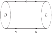
Figure 1: The leading order contribution to heavy-to-light form factors with “s” representing the soft momentum.

The momenta for $\bar{B}$ and light meson are denoted by $P$ and $P^{\prime}$, respectively. It is convenient to work in the $\bar{B}$ meson rest frame and set $P^{\prime}_{\bot}=0$. In this Lorentz frame, the momentum transfer $q$ is purely longitudinal, i.e., $q_{\bot}=0$ and $q^{2}=q^{+}q^{-}\geq 0$ covers the entire physical range.

The lowest order contribution to the form factor comes from the soft Feynman diagram where the spectator antiquark goes directly into the final light meson. The diagram is depicted in Fig. 1. The valence quark approximation guarantees that only the endpoint wave function of the light meson overlaps with the $\bar{B}$ meson. We use $p_{b}$, $p_{1}$ and $p_{q}$ to denote the momentum of the $b$ quark, the energetic quark and the spectator:

$$p_{b}^{+}=(1-x)P^{+},\qquad\qquad p_{b\perp}=-k_{\perp},$$

$$p_{1}^{+}=(1-x^{\prime})P^{\prime+},\qquad~{}~{}~{}~{}p_{1\perp}=-k_{\perp},$$

$$p_{q}^{+}=xP^{+}=x^{\prime}P^{\prime+},\qquad~{}~{}p_{q\perp}=k_{\perp},$$ (28)

where $P^{+}=M_{B}$ and $P^{\prime+}=2E$. The $x$, $x^{\prime}$ are the momentum fractions of the spectator antiquark in $\bar{B}$ meson and in the final state meson, respectively. $x$ and $x^{\prime}$ are connected by $x=x^{\prime}r$. It is useful to define a variable $r\equiv P^{\prime+}/P^{+}=1-q^{2}/M_{B}^{2}$. Since $x^{\prime}$ varies from 0 to 1, thus $x$ varies from 0 to $r$.

Now, we are able to present the derivation of form factors in light cone approach with some details. The $\bar{B}$ to pseudoscalar meson matrix element can be expressed as

$$\langle P|\bar{\xi}h_{v}|\bar{B}\rangle=(-1)N_{c}\int^{r}_{0}dx\int\frac{d^{2}k_{\perp}}{2(2\pi)^{3}}P^{+}\phi_{P}^{*}(x^{\prime},k_{\perp})\phi_{B}(x,k_{\perp})\frac{P^{+}P^{\prime+}\sqrt{x(1-x)}\sqrt{x^{\prime}(1-x^{\prime})}}{\sqrt{2}\tilde{M}_{0}\sqrt{2}\tilde{M}_{0}^{\prime}}$$

$$\times\mbox{Tr}\left[\frac{(\hbox to0.0pt{\hskip 0.85355pt/\hss}{p}_{q}-m_{q})}{p_{q}^{+}}\frac{(i\gamma_{5})}{\sqrt{N_{c}}}\frac{\hbox to0.0pt{\hskip 0.28436pt/\hss}{n}_{-}}{2}(1+\hbox to0.0pt{/\hss}{v})\frac{(-i\gamma_{5})}{\sqrt{N_{c}}}\right],~{}~{}~{}~{}~{}~{}~{}~{}~{}~{}~{}~{}$$ (29)

where $m_{q}$ is the mass of spectator antiquark. Since $x\sim x^{\prime}\sim\Lambda_{\rm QCD}/m_{b}$, we will neglect $x,x^{\prime}$ compared to $1$. The mass difference between $b$ quark mass and $\bar{B}$ meson is neglected, i.e., $m_{b}\doteq M_{B}$. It is easy to obtain the relation $\sqrt{x(1-x)}\tilde{M}_{0}=\sqrt{{\cal A}^{2}+k_{\bot}^{2}}$. Expanding the momentum and keeping the leading power component, we get

$$\langle P|\bar{\xi}h_{v}|\bar{B}\rangle=\int^{r}_{0}dx\int\frac{d^{2}k_{\perp}}{2(2\pi)^{3}}\frac{\phi_{P}^{*}(x^{\prime},k_{\perp})\phi_{B}(x,k_{\perp})}{\sqrt{{\cal A}_{B}^{2}+k_{\perp}^{2}}\sqrt{{\cal A}_{P}^{2}+k_{\perp}^{2}}}~{}xm_{b}^{2}(p_{q}^{-}+m_{q}),$$ (30)

where $p_{q}^{-}=\frac{k_{\bot}^{2}+m_{q}^{2}}{xm_{b}}$. From Eqs. (II.1) and (30), one obtain

$$\zeta_{P}=\frac{m_{b}}{2E}\int^{r}_{0}dx\int\frac{d^{2}k_{\perp}}{2(2\pi)^{3}}\frac{\phi^{*}_{P}(x^{\prime},k_{\perp})\phi_{B}(x,k_{\perp})}{\sqrt{{\cal A}_{B}^{2}+k_{\perp}^{2}}\sqrt{{\cal A}_{P}+k_{\perp}^{2}}}(xm_{b}m_{q}+m_{q}^{2}+k_{\perp}^{2}).$$ (31)

It shows that the leading order form factor $\zeta_{P}$ depends on the spectator quark mass $m_{q}$, scaleless factor $m_{b}/E$ and non-perturbatively depends on $E$ through light meson wave function $\phi_{P}(x^{\prime},k_{\bot})$ at $x^{\prime}\sim\Lambda_{\rm QCD}/E$. The $m_{b}$ must be associated with $x$ means that the form factor depends on the non-perturbative scale $X=xm_{b}$ rather than hard scale $m_{b}$ (except a normalization constant factor $\sqrt{m_{b}}$).

For $\bar{B}$ meson decays to longitudinal polarized vector, substituting the polarization vector into the right hand side of eq. (II.1), we get

$$\langle V|\bar{\xi}\gamma_{5}h_{v}|\bar{B}\rangle=-iM_{V}\zeta_{||}(\frac{P^{\prime+}}{M_{V}}-\frac{M_{V}}{P^{\prime+}})=-iP^{\prime+}\zeta_{||},$$ (32)

where we have dropped the sub-leading term. The expression in the light cone approach gives

$$\langle V|\bar{\xi}\gamma_{5}h_{v}|\bar{B}\rangle = i\int_{0}^{r}dx\int\frac{d^{2}k_{\perp}}{2(2\pi)^{3}}\frac{\phi_{V}^{*}(x^{\prime},k_{\perp})\phi_{B}(x,k_{\perp})}{2\sqrt{{\cal A}_{B}^{2}+k_{\perp}^{2}}\sqrt{{\cal A}_{V}^{2}+k_{\perp}^{2}}}x^{\prime}m_{b}^{2}$$

$$\times\mbox{Tr}\left[(\hbox to0.0pt{\hskip 0.85355pt/\hss}{p}_{q}-m_{q})\left(-\hat{\epsilon}\!\!/+\frac{\hat{\epsilon}\cdot(p_{1}-p_{q})}{W_{V}}\right)\frac{\hbox to0.0pt{\hskip 0.28436pt/\hss}{n}_{-}}{2}\gamma_{5}(1+\hbox to0.0pt{/\hss}{v})\gamma_{5}\right],$$

$$= \frac{-im_{b}^{2}P^{\prime+}}{2}\int^{r}_{0}dx\int\frac{d^{2}k_{\perp}}{2(2\pi)^{3}}\frac{\phi_{V}^{*}(x^{\prime},k_{\perp})\phi_{B}(x,k_{\perp})}{M_{0V}\sqrt{{\cal A}_{B}^{2}+k_{\perp}^{2}}\sqrt{{\cal A}_{V}^{2}+k_{\perp}^{2}}}$$ (33)

$$\times x[2z^{2}(p_{q}^{+}+m_{q})+\frac{p_{q}^{-}+z^{2}p_{1}^{+}}{W_{V}}(p_{q}^{-}+m_{q})],$$

with $z\equiv M_{0V}/P^{\prime+}$. Although it seems that the first term is suppressed by $\lambda=\sqrt{\Lambda_{QCD}/m_{b}}$, later we find that this term gives a relatively large contribution in the numerical calculation. We obtain the expression for the longitudinal leading order form factor as

$$\zeta_{||} = \frac{m_{b}^{2}}{2}\int\frac{dxd^{2}k_{\perp}}{2(2\pi)^{3}}\frac{\phi_{V}^{*}(x^{\prime},k_{\perp})\phi_{B}(x,k_{\perp})}{M_{0V}\sqrt{{\cal A}^{2}_{B}+k_{\perp}^{2}}\sqrt{{\cal A}_{V}^{2}+k_{\perp}^{2}}}$$ (34)

$$\times x\left[2z^{2}(p_{q}^{+}+m_{q})+\frac{p_{q}^{-}+z^{2}rm_{b}}{W_{V}}(p_{q}^{-}+m_{q})\right].$$

Similarly, we can analyze the leading order transverse form factor. When performing the calculation of $\zeta_{\perp}$, a formula for the transverse momentum integral is useful

$$\int d^{2}k_{\perp}(\epsilon\cdot p_{1})p_{q}^{\alpha}=\frac{1}{2}\int d^{2}k_{\perp}k_{\perp}^{2}\epsilon^{\alpha}.$$ (35)

The expression for $\bar{B}$ to transversely polarized vector meson is

$$\langle V|\bar{\xi}\gamma_{\bot}^{\mu}h_{v}|\bar{B}\rangle = i\int_{0}^{r}dx\int\frac{d^{2}k_{\perp}}{2(2\pi)^{3}}\frac{\phi_{V}^{*}(x^{\prime},k_{\perp})\phi_{B}(x,k_{\perp})}{2\sqrt{{\cal A}_{B}^{2}+k_{\perp}^{2}}\sqrt{{\cal A}_{V}^{2}+k_{\perp}^{2}}}xm_{b}^{2}$$

$$\times\mbox{Tr}\left[(\hbox to0.0pt{\hskip 0.85355pt/\hss}{p}_{q}-m_{q})\left(-\hat{\epsilon}\!\!/+\frac{\hat{\epsilon}\cdot(p_{1}-p_{q})}{W_{V}}\right)\frac{\hbox to0.0pt{\hskip 0.28436pt/\hss}{n}_{-}}{2}\gamma_{\bot}^{\mu}(1+\hbox to0.0pt{/\hss}{v})\gamma_{5}\right],$$

$$= -m_{b}^{2}\int\frac{dxd^{2}k_{\perp}}{2(2\pi)^{3}}\frac{\phi_{V}^{*}(x^{\prime},k_{\perp})\phi_{B}(x,k_{\perp})}{\sqrt{{\cal A}_{B}^{2}+k_{\perp}^{2}}\sqrt{{\cal A}_{V}^{2}+k_{\perp}^{2}}}\epsilon^{\mu\nu\rho\sigma}\epsilon_{\nu}^{*}v_{\rho}n_{-\sigma}~{}x(p_{q}^{-}+m_{q}+\frac{k_{\perp}^{2}}{W_{V}}).$$

It is straightforward to get:

$$\zeta_{\perp} = \frac{m_{b}^{2}}{2E}\int\frac{dxd^{2}k_{\perp}}{2(2\pi)^{3}}\frac{\phi_{V}^{*}(x^{\prime},k_{\perp})\phi_{B}(x,k_{\perp})}{\sqrt{{\cal A}_{B}^{2}+k_{\perp}^{2}}\sqrt{{\cal A}_{V}^{2}+k_{\perp}^{2}}}~{}x(p_{q}^{-}+m_{q}+\frac{k_{\perp}^{2}}{W_{V}}).$$ (37)

II.4 Higher order corrections to the heavy-to-light form factors in the light cone perturbation theory

In this subsection, we will derive the higher order corrections for the heavy to light form factors in the light cone perturbation theory of QCD. Besides the leading order soft contributions to the universal form factors, the next-to-leading order contribution is the kind of diagrams shown in Fig. 2 with one hard gluon exchange (about the vertex corrections, see BF1 ; SCETff1 ).

A four-component Dirac field $\psi$ can be decomposed into two-component spinors $\xi$ and $\eta$ by

$$\psi=\xi+\eta,\qquad\xi\equiv P_{-}\psi=\frac{\hbox to0.0pt{\hskip 0.28436pt/\hss}{n}_{-}\hbox to0.0pt{\hskip 0.28436pt/\hss}{n}_{+}}{4}\psi,\qquad\eta\equiv P_{+}\psi=\frac{\hbox to0.0pt{\hskip 0.28436pt/\hss}{n}_{+}\hbox to0.0pt{\hskip 0.28436pt/\hss}{n}_{-}}{4}\psi,$$ (38)

with equations of motion for spinors $\xi$ and $\eta$ are

$$in_{-}\cdot D\frac{\hbox to0.0pt{\hskip 0.28436pt/\hss}{n}_{+}}{2}~{}\xi+(i\hbox to0.0pt{\hskip 2.27626pt/\hss}{D}_{\bot}-m)\eta=0;$$ (39)

$$in_{+}\cdot D\frac{\hbox to0.0pt{\hskip 0.28436pt/\hss}{n}_{-}}{2}~{}\eta+(i\hbox to0.0pt{\hskip 2.27626pt/\hss}{D}_{\bot}-m)\xi=0.$$ (40)

In light cone quantization, the time variable is chosen to be different from the conventional one $t=x^{3}$. We adopt the light cone time as $\tau=n_{+}\cdot x$ and then the time-like derivative is $n_{-}\cdot\partial$. In Eq. (40), there is no time derivative. Thus $\eta$ is a constrained field, since it is determined by $\xi$ at any time of $n_{+}\cdot x$. From Eq. (40), $\eta$ field is obtained as

$$\eta=\frac{1}{in_{+}\cdot D}(i\hbox to0.0pt{\hskip 2.27626pt/\hss}{D}_{\bot}+m)\frac{\hbox to0.0pt{\hskip 0.28436pt/\hss}{n}_{+}}{2}\xi.$$ (41)

For the gluon field, it satisfies the color Maxwell equation $\partial_{\mu}F^{a\mu\nu}=gJ^{a\nu}$ where $J^{a\nu}$ is the quark current. By using the constraint $n_{+}\cdot A=0$, we obtain one relation $(n_{+}\cdot\partial)\partial_{\mu}A^{a\mu}=-g(n_{+}\cdot J^{a})$. Thus, the field component $n_{-}\cdot A$ is not a dynamical variable but determined by $A_{\bot}$ through

$$n_{-}\cdot A=\frac{2}{n_{+}\cdot\partial}\partial_{\bot}\cdot A_{\bot}-\frac{2}{(n_{+}\cdot\partial)^{2}}g(n_{+}\cdot J^{a}).$$ (42)

The Feynman rules for $\xi$ and $A_{\bot}$ have been derived, such as in SB which are not useful for our purpose. We prefer to use another formulation given in LB . In light cone perturbation theory, the diagrams are $n_{+}\cdot x$-ordered and all particles are on mass-shell. For the propagator of quark, it contains an instantaneous part, in particular

$$\frac{i(\hbox to0.0pt{\hskip 0.85355pt/\hss}{p}+m)}{p^{2}-m^{2}+i\epsilon}=\frac{i(\hbox to0.0pt{\hskip 0.85355pt/\hss}{p}_{on}+m)}{p^{2}-m^{2}+i\epsilon}+\frac{i~{}\hbox to0.0pt{\hskip 0.28436pt/\hss}{n}_{+}}{2n_{+}\cdot p},$$ (43)

where $p_{on}$ is the on-shell momentum $p_{on}=(n_{-}\cdot p,\frac{p_{\bot}^{2}+m^{2}}{n_{-}\cdot p},p_{\bot})$ and $p_{on}^{2}=m^{2}$. The second term in the quark propagator $\frac{\hbox to0.0pt{\hskip 0.28436pt/\hss}{n}_{+}}{2n_{+}\cdot p}$ is the instantaneous part induced by integrating out the field $\eta$. For the gluon field, the polarization sum is written as

$$d_{\mu\nu}(k)\equiv\sum\limits_{\lambda_{g}}\epsilon_{\mu}(k,\lambda_{g})\epsilon_{\nu}^{*}(k,\lambda_{g})=\sum\limits_{i=1,2}\left[-n_{+\mu}\frac{\epsilon^{(i)}\cdot k}{n_{+}\cdot k}+\epsilon^{(i)}_{\mu}\right]\left[-n_{+\nu}\frac{\epsilon^{(i)}\cdot k}{n_{+}\cdot k}+\epsilon^{(i)}_{\nu}\right],$$ (44)

where $\epsilon^{(i)}$ are purely transverse vectors: $\epsilon^{(i)+}=\epsilon^{(i)-}=0$ and $\epsilon^{(i)*}_{\bot}\cdot\epsilon^{(j)}_{\bot}=\delta^{ij}$. There are two terms in the bracket of Eq. (44): the first term $n_{+\mu}\frac{\epsilon^{(i)}\cdot k}{n_{+}\cdot k}$ comes from the longitudinal component $n_{+}\cdot A$ and the second $\epsilon^{(i)}_{\mu}$ from the transverse component $A_{\bot}$. If the gluon momentum is chosen to be in the longitudinal direction, then $\epsilon^{(i)}\cdot k=0$ and only the transverse components $\epsilon^{(i)}$ are remained. It reflects the fact that the physical gluon is transverse polarized. In the above rules, the choice of $n_{+}$ and $n_{-}$ is arbitrary and there is a symmetry by exchanging them. In this way, we obtain the light cone quantization rules for the light cone time $n_{-}\cdot x$.

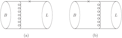
Figure 2: The one gluon exchange contributions to heavy-to-light form factors with the signs “$\times$” representing electro-weak vertex.

For the one gluon exchange diagram given in Fig. 2, the amplitude at the quark level is given in the conventional covariant form as

$$A=\frac{g^{2}}{k^{2}}d_{\mu\nu}\left\{\bar{u}(p_{1})\Gamma\frac{(\hbox to0.0pt{\hskip 0.85355pt/\hss}{p}_{q1}+m_{b})}{p_{q1}^{2}-m_{b}^{2}}T^{A}\gamma^{\mu}b(p_{b})~{}\bar{v}_{s}(p_{q})T^{A}\gamma^{\nu}v(p_{2})~{}~{}~{}\right.$$

$$\left.+\bar{u}(p_{1})T^{A}\gamma^{\mu}\frac{\hbox to0.0pt{\hskip 0.85355pt/\hss}{p}_{q2}}{p_{q2}^{2}}\Gamma b(p_{b})~{}\bar{v}_{s}(p_{q})T^{A}\gamma^{\nu}v(p_{2})\right\},$$ (45)

where $u(v)$ are light quark (antiquark) spinor, $b(v_{s})$ are $b$ quark (spectator antiquark) spinor; $p_{q1,q2}$ are the internal quark momenta, $k$ the exchanged gluon momentum, and $k=p_{2}-p_{q}$, $p_{q1}=p_{b}-p_{2}$, $p_{q2}=p_{1}+p_{2}-p_{q}$. The first term of the amplitude comes from contribution of Fig. 2(a) and the second term from the diagram Fig. 2(b). We have neglected the light quark masses. For the second term in Eq. (II.4), we use the light cone quantization rules of Eqs. (43,44). While for the first term in Eq. (II.4), the exchanged rules of Eqs. (43,44) by $n_{-}\leftrightarrow n_{+}$ is applied. Thus, the amplitude is rewritten in the light cone form by

$$A=\frac{g^{2}}{k^{2}}\left\{\bar{u}\Gamma\left[\frac{\hbox to0.0pt{\hskip 0.28436pt/\hss}{n}_{-}}{2n_{-}\cdot p_{q1}}+\frac{(\hbox to0.0pt{\hskip 0.85355pt/\hss}{p}_{q1})_{on}+m_{b}}{p_{q1}^{2}-m_{b}^{2}}\right]T^{A}\left[\gamma_{\bot}^{\mu}-\frac{\hbox to0.0pt{\hskip 0.28436pt/\hss}{n}_{-}}{n_{-}\cdot k}k_{\bot}^{\mu}\right]b~{}\bar{v}_{s}T^{A}\left[\gamma_{\bot\mu}-\frac{\hbox to0.0pt{\hskip 0.28436pt/\hss}{n}_{-}}{n_{-}\cdot k}k_{\bot\mu}\right]v\right.$$

$$+\left.\bar{u}T^{A}\left[\gamma_{\bot}^{\mu}-\frac{\hbox to0.0pt{\hskip 0.28436pt/\hss}{n}_{+}}{n_{+}\cdot k}k_{\bot}^{\mu}\right]\left[\frac{\hbox to0.0pt{\hskip 0.28436pt/\hss}{n}_{+}}{2n_{+}\cdot p_{q2}}+\frac{(\hbox to0.0pt{\hskip 0.85355pt/\hss}{p}_{q2})_{on}}{p_{q2}^{2}}\right]\Gamma b~{}\bar{v}_{s}T^{A}\left[\gamma_{\bot\mu}-\frac{\hbox to0.0pt{\hskip 0.28436pt/\hss}{n}_{+}}{n_{+}\cdot k}k_{\bot\mu}\right]v\right\}.$$ (46)

Neglecting the contributions suppressed by $\Lambda_{\rm QCD}/m_{b}$, we find the contribution from the instantaneous interaction part is

$$A^{h}=\frac{-g^{2}}{(n_{+}\cdot p_{2})(n_{-}\cdot p_{q})}\left\{\bar{\xi}_{n_{-}}\Gamma\frac{\hbox to0.0pt{\hskip 0.28436pt/\hss}{n}_{-}}{2m_{b}}T^{A}\gamma_{\bot}^{\mu}h_{v}~{}\bar{v}_{s}T^{A}\gamma_{\bot\mu}\xi_{n_{-}}+\bar{\xi}_{n_{-}}T^{A}\gamma_{\bot}^{\mu}\frac{\hbox to0.0pt{\hskip 0.28436pt/\hss}{n}_{+}}{2n_{+}\cdot P^{\prime}}\Gamma h_{v}~{}\bar{v}_{s}T^{A}\gamma_{\bot\mu}\xi_{n_{-}}\right\}.$$ (47)

This contribution is not singular for the leading twist distribution amplitudes of $B$ and light mesons. It is usually called “hard” contribution which breaks the spin symmetry due to $\hbox to0.0pt{\hskip 0.28436pt/\hss}{n}_{-}$ and $\hbox to0.0pt{\hskip 0.28436pt/\hss}{n}_{+}$ matrices. In the light cone language, the hard gluon exchange contributions come from the instantaneous quark interactions and the transversely polarized gluons. The hard one gluon exchange contributions can not be absorbed into the three universal form factors because this type higher order contributions break the spin symmetry in the leading order.

III Numerical Results and Discussions

The physical heavy-to-light form factors contain both hard and soft contributions. In this study, we concentrate on the leading order soft form factors. The next-to-leading order $\alpha_{s}$ corrections, which breaks the spin symmetry, will be calculated in a future work. In order to obtain the numerical results, we have to determine the wave functions of the hadrons which contain all information of the hadron state. The full solution needs great efforts, so we use the phenomenological Gaussian-type wave function:

$$\phi(x,k_{\perp})=N\sqrt{\frac{dk_{z}}{dx}}\mbox{exp}(-\frac{\vec{k}^{2}}{2\omega^{2}}),$$ (48)

where $N=4(\pi/\omega^{2})^{3/4}$ and $k_{z}$ of the internal momentum $\vec{k}=(\vec{k}_{\perp},k_{z})$ is defined through

$$1-x=\frac{e_{1}-k_{z}}{e_{1}+e_{2}},\qquad x=\frac{e_{2}+k_{z}}{e_{1}+e_{2}},$$ (49)

with $e_{i}=\sqrt{m_{i}^{2}+\vec{k}_{i}^{2}}=\frac{x_{i}M_{0}}{2}+\frac{m_{i}^{2}+k_{\perp i}^{2}}{2x_{i}M_{0}}$. We then have

$$k_{z}=\frac{xM_{0}}{2}-\frac{m_{2}^{2}+k_{\perp}^{2}}{2xM_{0}},\qquad\frac{dk_{z}}{dx}=\frac{e_{1}e_{2}}{x(1-x)M_{0}}.$$ (50)

In this wave function, the distribution of the momentum is determined by the quark mass and the parameter $\omega$. The quarks are constituent quarks and the quark masses are usually chosen as:

$$m_{u,d}=0.25{\mbox{ GeV}},\qquad m_{s}=0.40{\mbox{ GeV}},\qquad m_{b}=4.8\mbox{ GeV}.$$ (51)

The parameter $\omega$ can be determined by the hadronic results, for example, the decay constants flavor .

As for the decay constants of $\eta$ and $\eta^{\prime}$, we should pay much more attention on the mixing of these two particles. Although the quark model has achieved great successes, we still don’t have the definite answer on the exact components of these two mesons. The study of $B$ to $\eta^{(\prime)}$ decays, especially the study on $B\to\eta^{(\prime)}$ form factor, can help us to understand their intrinsic characters (For a recent study, please see CKL ). Here we view these two particles as the conventional two quark states. As for the mixing, we use the quark flavor basis proposed by Feldmann and Kroll FKmixing , i.e. these two mesons are made of $\eta_{n}=\bar{n}n=(\bar{u}u+\bar{d}d)/\sqrt{2}$ and $\eta_{s}=\bar{s}s$:

$$\left(\begin{array}[]{c}|\eta\rangle\\ |\eta^{\prime}\rangle\end{array}\right)=U(\phi)\left(\begin{array}[]{c}|\eta_{n}\rangle\\ |\eta_{s}\rangle\end{array}\right)\;,$$ (52)

with the mixing matrix,

$$U(\phi)=\left(\begin{array}[]{cc}\cos\phi&~{}-\sin\phi\\ \sin\phi&\phantom{~{}-}\cos\phi\end{array}\right)\;,$$ (53)

where $\phi$ is the mixing angle. In this mixing scheme, only two decay constants $f_{n}(n=u,d)$ and $f_{s}$ are needed:

$$\langle 0|\bar{n}\gamma^{\mu}\gamma_{5}n|\eta_{n}(P)\rangle = \frac{i}{\sqrt{2}}\,f_{n}\,P^{\mu}\;,$$

$$\langle 0|\bar{s}\gamma^{\mu}\gamma_{5}s|\eta_{s}(P)\rangle = if_{s}\,P^{\mu}\;.$$ (54)

This is based on the assumption that the intrinsic $\bar{n}n(\bar{s}s)$ component is absent in the $\eta_{s}(\eta_{n})$ meson, i.e., based on the $OZI$ suppression rule. These decay constants have been determined from the related exclusive processes as FKmixing :

$$f_{n}=(1.07\pm 0.02)f_{\pi},\qquad f_{s}=(1.34\pm 0.06)f_{\pi}.$$ (55)

In the following we will calculate the form factors of $B\to\eta_{n}$ and $B_{s}\to\eta_{s}$. The gluonic contribution to $B\to\eta^{(\prime)}$ has also been studied in Ref. CKL . We will neglect it as it is very small.

We use the following results for the decay constants as input in the light front wave functions:

$$f_{B}=0.190\mbox{ GeV},~{} f_{B_{s}}=0.236\mbox{GeV},~{}~{}f_{\pi}=0.132\mbox{ GeV},~{} f_{K}=0.160\mbox{ GeV},~{}$$

$$f_{\rho}=0.205{\mbox{ GeV}},~{} f_{\omega}=0.195\mbox{GeV},~{}~{}~{}~{}f_{K^{\star}}=0.217\mbox{ GeV},~{} f_{\phi}=0.231\mbox{ GeV}.$$ (56)

Then the parameters $\omega$ in the light-front wave functions are determined from these decay constants as:

$$\omega_{B}=0.55^{+0.05}_{-0.04}\mbox{GeV},\qquad\qquad\omega_{B_{s}}=0.64^{+0.05}_{-0.06}\mbox{GeV},$$

$$\omega_{\pi}=0.33\mbox{GeV},\qquad\qquad\qquad\omega_{K}=0.38\mbox{GeV},$$

$$\omega_{n}=0.38^{+0.09}_{-0.08}\mbox{GeV},\qquad\qquad\omega_{s}=0.39^{+0.06}_{-0.06}\mbox{GeV},$$

$$\omega_{\rho}=0.31^{+0.03}_{-0.03}\mbox{GeV},\qquad\qquad\omega_{\omega}=0.29^{+0.03}_{-0.03}\mbox{GeV},$$

$$\omega_{K^{\star}}=0.33^{+0.03}_{-0.03}\mbox{GeV},~{}~{}~{}\qquad\ \omega_{\phi}=0.35^{+0.03}_{-0.03}\mbox{GeV},$$ (57)

where the uncertainties come from varying the decay constants of the heavy and the light mesons by $10\%$. Some light meson decay constants have been determined to a high accuracy, for example, $f_{\pi}$, $f_{K}$. We neglect the uncertainties for them.

III.1 Results for $B\to P$ form factor $\zeta_{P}$

Now we are ready to give the numerical results of the $B$ to pseudoscalar soft form factors at $q^{2}=0$, i.e. $E=m_{B}/2$. Using the above parameters, we obtain the results as follows:

$$\zeta_{P}^{B\to\pi}(\frac{m_{B}}{2})=0.247,~{}\qquad\qquad\zeta_{P}^{B\to K}(\frac{m_{B}}{2})=0.297,$$

$$\zeta_{P}^{B\to\eta_{n}}(\frac{m_{B}}{2})=0.287^{+0.059}_{-0.065},$$

$$\zeta_{P}^{B_{s}\to K}(\frac{m_{B}}{2})=0.290,\qquad\qquad\zeta_{P}^{B_{s}\to\eta_{s}}(\frac{m_{B}}{2})=0.288^{+0.047}_{-0.052},$$ (58)

where the uncertainties are from the decay constant of the light mesons. We also find the uncertainties caused by $B$ meson decay constants are rather small and thus we neglect these uncertainties. In Ref. SCETLCSR1 , the SCET sum rule result is calculated as $\zeta_{P}^{B\to\pi}=0.27$ which is consistent with our result within theoretical errors. The physical form factors can be obtained directly using the relation in Eq. (7). At maximally recoil $r=1$, $f_{+}$ and $f_{0}$ are equal to each other, which are exactly the soft form factor $\zeta_{P}$; $f_{T}$ is slightly larger. Table 1 lists the $B\to P$ form factors at $q^{2}=0$.

Figure 3: The $q^{2}$ dependence of $B_{(s)}\to P$ form factors. In this figure, we plot $f_{+}$, $f_{0}$ and $f_{T}$ for $B\to\pi$, $B\to K$ and $B_{s}\to K$ transitions. But for $B\to\eta_{n}$ and $B_{s}\to\eta_{s}$, only the first two form factors are shown for the ambiguity of the mass for $\eta_{n}$ and $\eta_{s}$ in $f_{T}$.

Table 1: The physical $B_{(u,d,s)}\to P$ form factors at maximally recoil using the usual LCQM CCH2 , LCSR BZpseudo , LQCD LQCD1 ; LQCD2 ; LQCD3 and PQCD PQCD approaches. The different values for $f_{+}(B\to\pi)$ in Ref. LQCD2 correspond to different extrapolations.

		LCQMCCH2	LCSRBZpseudo	PQCD PQCD	LQCDLQCD1	LQCD LQCD2	LQCDLQCD3	This work
$B\to\pi$	$f_{+}$	$0.25$	$0.258$	$0.292$	$0.27$	$0.27(0.26)$	$0.23$	$0.247$
	$f_{T}$		$0.253$	$0.278$				$0.253$
	$f_{0}$	$0.25$		$0.292$	$0.27$			$0.247$
$B\to K$	$f_{+}$	$0.35$	$0.331$	$0.321$				$0.297$
	$f_{T}$		$0.358$	$0.311$				$0.325$
	$f_{0}$	$0.35$		$0.321$				$0.297$
$B\to\eta_{n}$	$f_{+}$		$0.275$					$0.287$
	$f_{T}$		$0.285$
	$f_{0}$							$0.287$
$B_{s}\to K$	$f_{+}$							$0.290$
	$f_{T}$							$0.317$
	$f_{0}$							$0.290$
$B_{s}\to\eta_{s}$	$f_{+}$							$0.288$
	$f_{0}$							$0.288$

These $B\to P$ form factors have also been studied systemically in the usual light-cone quark model CCH1 ; CJK ; CCH2 , the light cone sum rules BZpseudo and PQCD approach PQCD . Although Lattice QCD cannot give direct predictions on the $B$ to light form factors at large recoiling, there are some studies using the extrapolations from the results at large $q^{2}$: in quenched LQCD LQCD1 and in unquenched LQCD LQCD2 ; LQCD3 . We cite these results in Table 1.

Comparing the results in Table 1, we can find that our leading-order results agree with the results calculated using other approaches. The numerical results of higher order corrections which should be small in our approaches will be taken into account in future work.

We compare our approach with the previous light cone quark models. As in the conventional form of CCH1 where the quarks are on-shell, the calculation of form factors are in the physical momentum regions $q^{2}\geq 0$. The difference between the approach in CCH1 and ours is that we make approximations in the heavy quark mass and large energy limit. The consistency of the numerical predictions in the two methods means that our result is the leading dominant contribution. In the covariant form in Jaus2 , the quarks are off-shell. The evaluations are performed in the momentum regions $q^{2}<0$ and the analytic continuation is required to obtain the physical form factors. The advantage of this approach is that the zero-mode $(k^{+}=0)$ contribution does not occur. In our method, the zero-mode contribution vanish in the heavy quark mass and large energy limit.

Since our analysis is within the SCET framework, we should make sure that the final state meson is energetic. The energy of the light meson should be larger than $\sqrt{m_{B}\Lambda_{QCD}}\sim 1.5\mbox{ GeV}$ in order to ensure it as a collinear meson. From this constraint, we can get $q^{2}=m_{B}^{2}-2m_{B}E<10\mbox{ GeV}^{2}$. Thus we can directly calculate the form factors in the range of $0<q^{2}<10\mbox{ GeV}^{2}$ and the results should be reliable. We plot the $q^{2}$ dependence of the $B_{(s)}\to P$ form factors in Fig. 3. In this figure, the form factors $f_{+}(q^{2})=\zeta_{P}(E)$, $f_{T}(q^{2})=\frac{M_{B}+M_{P}}{M_{B}}\zeta_{P}(E)$ and $f_{0}(q^{2})=\frac{2E}{m_{B}}\zeta_{P}(E)$ are plotted. The $q^{2}$ dependence of $f_{+}$ and $f_{T}$ are essentially the same except the only difference of the form factor at $q^{2}=0$. The curve of $f_{0}(q^{2})$ is more flat than the other two because of the compensation of the factor $r=\frac{2E}{m_{B}}=1-\frac{q^{2}}{m_{B}^{2}}$.

In order to study the analytic $q^{2}$ dependence of the results for the form factors, we fit the data by adopting the simple parametrization:

$$f(q^{2})=\frac{f(0)}{1-a(q^{2}/m_{B}^{2})+b(q^{2}/m_{B}^{2})^{2}},$$ (59)

where $f(0)$ are the results at $q^{2}=0$ which have been discussed as above, while $a$ and $b$ are the parameters. The fitted results for these two parameters are summarized in Table 2. From Fig. 3, we can see that all of the curves are close to be a straight line and the parameters $b$ should be rather small. The results from the parametrization also verify this expectation. Our results for parameters $a$ for different processes are also close to each other: around $a=1.5$ for $f_{+}$ and $f_{T}$ or $a=0.5$ for $f_{0}$.

Table 2: The parameters in the parametrization of $B_{(u,d,s)}\to P$ form factors. The fitted values of $a$ and $b$ for $f_{T}$ are the same with the ones in $f_{+}$.

		$f_{+}^{B\to\pi}$	$f_{+}^{B\to K}$	$f_{+}^{B\to\eta_{n}}$	$f_{+}^{B_{s}\to K}$	$f_{+}^{B_{s}\to\eta_{s}}$
$a$		$1.43$	$1.28$	$1.31$	$1.51$	$1.49$
$b$		$0.08$	$0.00$	$-0.00$	$0.23$	$0.22$
		$f_{0}^{B\to\pi}$	$f_{0}^{B\to K}$	$f_{0}^{B\to\eta_{n}}$	$f_{0}^{B_{s}\to K}$	$f_{0}^{B_{s}\to\eta_{s}}$
$a$		$0.56$	$0.46$	$0.48$	$0.66$	$0.64$
$b$		$-0.14$	$-0.08$	$-0.14$	$-0.00$	0.00

III.2 Results for $B\to V$ form factors

Similar analysis can also be applied to $B\to V$ form factors. At $q^{2}=0$, the results for the $B\to V$ soft form factors are

$$\zeta_{||}^{B\to\rho}(\frac{m_{B}}{2})=0.260^{+0.028}_{-0.030},~{}~{}\qquad\zeta_{\perp}^{B\to\rho}(\frac{m_{B}}{2})=0.260^{+0.030}_{-0.031},$$

$$\zeta_{||}^{B\to\omega}(\frac{m_{B}}{2})=0.240^{+0.029}_{-0.031},~{}~{}\qquad\zeta_{\perp}^{B\to\omega}(\frac{m_{B}}{2})=0.239^{+0.031}_{-0.031},$$

$$\zeta_{||}^{B\to K^{*}}(\frac{m_{B}}{2})=0.284^{+0.025}_{-0.027},\qquad\zeta_{\perp}^{B\to K^{*}}(\frac{m_{B}}{2})=0.290^{+0.027}_{-0.029},$$

$$\zeta_{||}^{B_{s}\to K^{*}}(\frac{m_{B}}{2})=0.279^{+0.030}_{-0.030},\qquad\zeta_{\perp}^{B_{s}\to K^{*}}(\frac{m_{B}}{2})=0.271^{+0.030}_{-0.030},$$

$$\zeta_{||}^{B_{s}\to\phi}(\frac{m_{B}}{2})=0.279^{+0.029}_{-0.030},~{}~{}\qquad\zeta_{\perp}^{B_{s}\to\phi}(\frac{m_{B}}{2})=0.276^{+0.030}_{-0.030},$$ (60)

where the uncertainties are from the decay constants of the light mesons. In order to make a comparison, we collect the results for the physical form factors in LCQM CCH1 ; CCH2 , LCSR BZvector , PQCD PQCD approach, LQCD LQCD1 ; LQCD4 and our leading-order results in Table 3. Our results are consistent with other approaches except for the smaller $T_{2,3}$ and larger $T_{1}$ in PQCD approaches.

Table 3: The physical $B\to V$ form factors at maximally recoil, i.e. $q^{2}=0$.

		$B\to\rho$	$B\to K^{*}$	$B\to\omega$	$B_{s}\to K^{*}$	$B_{s}\to\phi$
LCQMCCH2	$V$	$0.27$	$0.31$
	$A_{0}$	$0.28$	$0.31$
	$A_{1}$	$0.22$	$0.26$
	$A_{2}$	$0.20$	$0.24$
LCSRBZvector	$V$	$0.323$	$0.411$	$0.293$	$0.311$	$0.434$
	$A_{0}$	$0.303$	$0.374$	$0.281$	$0.360$	$0.474$
	$A_{1}$	$0.242$	$0.292$	$0.219$	$0.233$	$0.311$
	$A_{2}$	$0.221$	$0.259$	$0.198$	$0.181$	$0.234$
	$T_{2}$	$0.267$	$0.333$	$0.242$	$0.260$	$0.349$
PQCDPQCD	$V$	$0.318$	$0.406$	$0.305$
	$A_{0}$	$0.366$	$0.455$	$0.347$
	$A_{1}$	$0.25$	$0.30$	$0.24$
	$A_{2}$	$0.21$	$0.24$	$0.20$
LQCDLQCD1	$V$	$0.35$
	$A_{0}$	$0.30$
	$A_{1}$	$0.27$
	$A_{2}$	$0.26$
	$T_{1}$		$0.24$LQCD4
This work	$V$	$0.298$	$0.339$	$0.275$	$0.323$	$0.329$
	$A_{0}$	$0.260$	$0.283$	$0.240$	$0.279$	$0.279$
	$A_{1}$	$0.227$	$0.248$	$0.209$	$0.228$	$0.232$
	$A_{2}$	$0.215$	$0.233$	$0.198$	$0.204$	$0.210$
	$T_{1}$	$0.260$	$0.290$	$0.239$	$0.271$	$0.276$
	$T_{2}$	$0.260$	$0.290$	$0.239$	$0.271$	$0.276$
	$T_{3}$	$0.184$	$0.194$	$0.168$	$0.165$	$0.170$

The features of our results are:

• Our results of $\zeta_{||}$ and $\zeta_{\perp}$ for every meson are close to each other, which is mainly due to the similar wave function for the longitudinal and transverse polarizations.

• The physical form factors can be directly calculated by using the soft form factors. The kinematic factor as in Eq. (7) makes the physical form factors different. $V$ is the largest form factor which is enhanced by the factor $1+M_{V}/M_{B}$, while $T_{3}$ is smallest one for a minus term.

• The soft form factors of $B\to K^{*}$ is larger than that of $B\to\rho$ because the $s$ quark in $K^{*}$ meson carries more momentum than $d$ quark in $\rho$, which can induce more overlap of the $\bar{B}$ meson wave function and the light $K^{*}$ meson wave function. $\zeta_{||,\perp}^{B\to\omega}$ is smaller than $\zeta_{||,\perp}^{B\to\rho}$, which is a consequence of the fact the decay constant of $\omega$ is smaller than that of $\rho$.

• As we have discussed above, we keep the first term in $\zeta_{||}$, although it is suppressed by $\lambda=\sqrt{\Lambda_{QCD}/m_{b}}$. This term can not be neglected in the numerics as the suppression is not so effective: the $\zeta_{||}^{B\to\rho}$ without this term becomes:

  $$\zeta_{||}^{B\to\rho}(\frac{m_{B}}{2})=0.139,$$ (61)

  which is quite smaller than the result with it. This small $\zeta_{||}$ can lead to a small $A_{0}$ but a large $A_{2}$ and $T_{3}$.

Figure 4: The $q^{2}$ dependence of the $B_{(s)}\to V$ form factors.

The $q^{2}$ dependence ($0<q^{2}<10\mbox{ GeV}^{2}$) of the form factors are plotted in Fig. 4. The two form factors $V$ and $T_{1}$ have the same $q^{2}$ dependence except the different results at $q^{2}=0$ and both of them can be directly calculated by $\zeta_{\perp}(E)$. $A_{0}(q^{2})=\zeta_{||}(E)$ has similar $q^{2}$ dependence with $\zeta_{\perp}(E)$. When the $q^{2}$ gets large, $A_{0}$ is a little sharper than $V$ and $T_{1}$. The other four form factors are rather flat and are less sensitive to $q^{2}$. From the figure, we can see that the $A_{2}$ and $T_{3}$ show a tendency to decrease at large $q^{2}$, these two form factors may not be described by the above parametrization and so we will not fit them as in $B$ to pseudoscalar decays. We use the same parametrization to describe the $q^{2}$ dependence of the other form factors, and the results for the fitted parameters are given in Table 4. From the table, we can see that the parameters $a$ for various channels are close to each other: around $a=1.5$ for $\zeta_{||}(A_{0})$ and $\zeta_{\perp}(V,T_{1})$ or $a=0.5$ for $\frac{2E}{m_{B}}\zeta_{\perp}(A_{1},T_{2})$. Another interesting feature is that: for all form factors, the parameter $b$ is not large and the form factor is dominated by the monopole term.

Table 4: The parameters in the parametrization of $B\to V$ form factors.

		$\zeta_{||}^{B\to\rho}(A_{0})$	$\zeta_{||}^{B\to\omega}(A_{0})$	$\zeta_{||}^{B\to K^{*}}(A_{0})$	$\zeta_{||}^{B_{s}\to K^{*}}(A_{0})$	$\zeta_{||}^{B_{s}\to\phi}(A_{0})$
$a$		$1.56$	$1.60$	$1.51$	$1.74$	$1.73$
$b$		$0.17$	$0.22$	$0.14$	$0.47$	$0.41$
		$\zeta^{B\to\rho}_{\perp}(V,T_{1})$	$\zeta^{B\to\omega}_{\perp}(V,T_{1})$	$\zeta^{B\to K^{*}}_{\perp}(V,T_{1})$	$\zeta^{B_{s}\to K^{*}}_{\perp}(V,T_{1})$	$\zeta^{B_{s}\to\phi}_{\perp}(V,T_{1})$
$a$		$1.45$	$1.49$	$1.37$	$1.64$	$1.60$
$b$		$0.15$	$0.20$	$0.11$	$0.42$	$0.36$
		$\frac{2E}{m_{B}}\zeta^{B\to\rho}_{\perp}(A_{1},T_{2})$	$\frac{2E}{m_{B}}\zeta^{B\to\omega}_{\perp}(A_{1},T_{2})$	$\frac{2E}{m_{B}}\zeta^{B\to K^{*}}_{\perp}(A_{1},T_{2})$	$\frac{2E}{m_{B}}\zeta^{B_{s}\to K^{*}}_{\perp}(A_{1},T_{2})$	$\frac{2E}{m_{B}}\zeta^{B_{s}\to\phi}_{\perp}(A_{1},T_{2})$
$a$		$0.62$	$0.66$	$0.55$	$0.82$	$0.48$
$b$		$-0.11$	$-0.10$	$-0.05$	$0.08$	$0.04$

IV Conclusions

A light cone quark model within the soft collinear effective theory is constructed in this study. We calculated all the heavy-to-light $B_{(s)}\to P$ and $B_{(s)}\to V$ transition form factors at large recoil region. The three universal soft form factors are studied, in particular, the $B\to V$ form factors $\zeta_{||,\bot}$ are given for the first time. Our numerical results are in general consistent with other non-perturbative methods, such as light cone sum rules and quark models within the theoretical errors. The fact that our numerical results are close to the results by other methods supports that the leading order soft contribution is dominant in the light cone quark model. The theoretical uncertainties caused by the less known $B$ meson decay constants are small. The $q^{2}$ dependence of the $B\to P,V$ form factor is also studied in the range $0<q^{2}<10\mbox{ GeV}^{2}$.

References

- (1) For a review, see: M. Battaglia, et al., CERN-2003-002, hep-ph/0304132.
- (2) M. Wirbel, B. Stech, M. Bauer Z. Phys. C 29 (1985) 637.
- (3) A. Szczepaniak, E.M. Henley and S.J. Brodsky, Phys. Lett. B 243 (1990) 287-292.
- (4) W. Jaus, Phys. Rev. D 41, (1990) 3394;
- (5) H.-Y. Cheng, C.-Y. Cheung and C.-W. Hwang, Phys. Rev. D 55 1559 (1997).
- (6) H.-M. Choi, C.-R. Ji, and L.S. Kisslinger, Phys. Rev. D65 (2002) 074032.
- (7) H.-Y. Cheng, C.-K. Chua and C.-W. Hwang, Phys. Rev. D 69 (2004) 074025.
- (8) T.M. Aliev, A. Ozpineci and M. Savci, Phys. Rev. D56 (1997); Phys. Lett. B400 (1997) 194-205; A. Khodjamirian, et al. Phys. Lett. B 410 (1997) 275-284; P. Ball and V.M. Braun, Phys. Rev. D 55 (1997) 5561-5576; E. Bagan, P. Ball and V.M. Braun, Phys. Lett. B 417 (1998) 154-162; V.M. Braun, hep-ph/9801222; P. Ball, JHEP 9809 (1998) 005.
- (9) P. Ball and R. Zwicky, Phys. Rev. D 71 (2005) 014015.
- (10) P. Ball, and R. Zwicky, Phys. Rev. D 71 (2005) 014029.
- (11) R. Akhoury, G. Sterman and Y.P. Yao, Phys. Rev. D 50 (1994) 358-372; H.-n. Li and H.-L. Yu, Phys. Rev. Lett. 74 (1995) 4388-4391. T. Kurimoto, H.-n. Li and A.I. Sanda, Phys. Rev. D 65 (2002) 014007; Z.-T. Wei and M.-Z. Yang, Nucl. Phys. B 642 (2002) 263-289; C.H. Chen abd C.Q. Geng, Nucl.Phys. B636 (2002) 338-364; C.-D. Lu and M.-Z. Yang, Eur. Phys. J. C 28 (2003) 515-523.
- (12) J. Charles, A.L. Yaouanc, L. Oliver, O. Pene and J.C. Raynal, Phys. Rev. D 60 (1999) 014001.
- (13) N. Isgur and Mark B. Wise, Phys. Lett. B 232 (1989) 113; 237(1990) 527.
- (14) C.W. Bauer, S. Fleming, D. Pirjol and I.W. Stewart, Phys. Rev. D 63 (2001) 114020.
- (15) C.W. Bauer, D. Pirjol and I.W. Stewart, Phys. Rev. D 67 (2003) 071502.
- (16) M. Beneke, A.P. Chapovsky, M. Diehl and Th. Feldmann, Nucl. Phys. B 643 (2002) 431-476.
- (17) M. Beneke and T. Feldmann, Nucl. Phys. B 685 (2004) 249-296; B.O. Lange and M. Neubert, Nucl. Phys. B 690 (2004) 249-278; Erratum-ibid. B 723 (2005) 201-202.
- (18) R.J. Hill, Phys. Rev. D73 (2006) 014012.
- (19) K.M. Foley and G.P. Lepage, Nucl. Phys. Proc. Suppl. 119 (2003) 635.
- (20) C.T.H. Davies, K.Y. Wong and G.P. Lepage, hep-lat/0611009.
- (21) F. De Fazio, T. Feldmann and T. Hurth, Nucl. Phys. B 733 (2006) 1.
- (22) J.P. Lee, Phys. Lett. B632 (2006) 287.
- (23) J. Chay, C. Kim and A.K. Leibovich, Phys. Lett. B 628 (2005) 57.
- (24) S.J. Brodsky, H.C. Pauli and S.S. Pinsky, Phys. Rep. 301 (1998) 299.
- (25) G.P. Lepage and S.J. Brodsky, Phys. Rev. D 22 (1980) 2157.
- (26) W. Jaus, Phys. Rev. D44 (1991) 2851; 60 (1999) 054026.
- (27) C.-W. Hwang and Z.-T. Wei, arXiv: hep-ph/0609036.
- (28) D. Ebert, R.N. Faustov and V.O. Galkin Phys. Rev. D64 (2001) 094022.
- (29) M. Beneke and T. Feldmann, Nucl. Phys. B 592 (2001) 3-34.
- (30) K.G. Wilson, T.S. Walhout, A. Harindranath, W.-M. Zhang and R.J. Perry, Phys. Rev. D 49 (1994) 6720-6766.
- (31) C. Hayne and N. Isgur, Phys. Rev. D 25 (1982) 1944.
- (32) C.-Y. Cheung, W.-M. Zhang and G.-L. Lin, Phys. Rev. D 52 (1995) 2915-2925.
- (33) P.P. Srivastava and S.J. Brodsky, Phys. Rev. D 64 (2001) 045006.
- (34) For flavour symmetry breaking in pseudoscalar meson decay constants, please see this reference as a review: Cosmoparticle physics, M.Yu.Khlopov, World Scientific, 1999.
- (35) Y.Y. Charng, T. Kurimoto and H.n. Li, Phys. Rev. D 74 (2006) 074024.
- (36) Th. Feldmann and P. Kroll, Phys. Rev. D 58 (1998) 114006; Phys. Lett. B 449 (1999) 339; Int. J. Mod. Phys. A 15, 159(1999).
- (37) L.D. Debbio, J.M. Flynn, L. Lellouch and J. Nieves, UKQCD Collaboration, Phys. Lett. B 416 (1998) 392-401.
- (38) E. Gulez et al., HPQCD Collaboration, Phys. Rev. D 73 (2006) 074502.
- (39) M. Okamoto et al., Fermilab/MILC Collaboration, Nucl. Phys. Proc. Suppl. 140 (2005) 461.
- (40) D. Becirevic, V. Lubicz and F. Mescia, hep-ph/0611295.