Paramaterizations of inclusive cross sections for pion production in proton-proton collisions. II. Comparison to new data.

Abstract

A set of new, precise data have recently been made available by the NA49 collaboration for charged pion production in proton-proton and proton-Carbon reactions at 158 GeV. The current paper compares this new data to five currently available arithmetic parameterizations. Although a precise fit is not expected, two of the parameterizations do not work very well but the other three are able to provide a moderately good, but not precise fit to the proton-proton data. The best two of these three parameterizations are scaled to the proton-Carbon data and again provide a moderately good, but not precise fit.

I INTRODUCTION

The NA49 collaboration altpp ; altpc has recently completed a series of measurements for charged pion production in proton-proton ($pp$) and proton-Carbon ($pC$) collisions at a beam momentum of 158 GeV, corresponding to $\sqrt{s}=17$ GeV. This surpasses previous data in that the new data is of much higher precision and quality and can therefore be used to provide more precise tests of hadronic production models. The NA49 collaboration altpp ; altpc indicate that simple arithmetic parameterizations are unable to account for the fine structure seen in their data, and they therefore provide a numerical interpolation scheme. We agree with this. However arithmetic parameterizations are used in a wide variety of applications including simulation of particle physics experiments fernow , simulations of cosmic rays showers in the Earth atmosphere rao ; gaisser ; sokolsky , description of particle reactions relevant to astrophysics longair and predicting radiation environments inside spacecraft wilson . For those using such parameterizations it is of interest to know how they compare to the new precision NA49 data altpp ; altpc , even though a precision fit will not be possible. Blattnig, Swaminathan, Kruger, Ngom, and Norbury blattnig analysed a set of parameterizations currently available and compared to an extensive data set for both neutral and charged pion production in $pp$ collisions. It was concluded that the parameterization of Badhwar and Stephens badhwar provided the best overall description of charged pion production. It is interesting to see how this compares to the new data altpp .

The Blattnig et al parameterizations blattnig have also been used in a variety of astrophysical and astroparticle applications bernado ; santamaria ; kelner ; kamae-2005 ; kamae-2006 ; moskalenko ; prodanovic where the interest is in calculating the spectrum of gamma rays, electrons and neutrinos which result from the decay of pions produced in proton-proton interactions. For example, Bernado bernado used the high energy $pp\rightarrow\pi^{0}$ cross sections in order to calculate the $\gamma$-ray spectrum from microquasars. This spectrum can be measured using gamma ray telescopes on satellites. Pion production cross section parameterizations blattnig have also been used recently in nuclear and particle physics applications blume ; denterria2004 ; denterria-2005 ; denterria-a-2005 . The nuclear modification factor $R_{AA}$ is basically the ratio of a nucleus-nucleus cross section divided by a scaled nucleon-nucleon cross section. The behavior of $R_{AA}$ can be used to provide information on signatures of quark-gluon plasma formation blume ; denterria2004 ; denterria-2005 ; denterria-a-2005 . Pion parameterizations have been used for the proton-proton cross sections in these nuclear modification factors blume ; denterria2004 ; denterria-2005 ; denterria-a-2005 . Given such widespread use of pion production cross section parameterizations, we deem it worthwhile to test currently available parameterizations against new accelerator data. This is the aim of the present work.

The outline of the paper is as follows. We summarize the paramaterizations studied previously blattnig making note of necessary variable transformations needed to describe the NA49 altpp ; altpc data set. We then compare these parameterizations to the new data for $pp$ reactions. Therefore the present work is a continuation of the previous paper blattnig but applied to the new data. The parameterizations which are able to give a reasonable fit to the $pp$ data are then scaled and compared to the $pC$ data.

II Differential cross sections

II.1 Review of Kinematics

Consider the inclusive reaction

$$a+b\rightarrow c+X$$ (1)

where $c$ is the produced particle of interest and $X$ is anything. Throughout this paper we assume that all variables, such as all momenta, are evaluated in the center of momentum (CM) frame. The momentum of particle $c$ is denoted as $p$, and supposing that it comes out at angle $\theta$ to the beam direction, then the longitudinal and transverse components of momentum are

$$p_{z} \equiv p\cos\theta$$ (2)

$$p_{T} \equiv p\sin\theta$$ (3)

Feynman used a scaled variable instead of $p_{z}$ itself hagedorn ; roe ; collins ; perkins2 . The Feynman scaling variable is collins ; whitmore ; wong ; nagamiya ; giacomelli ; tannenbaum ; cassing

$$x_{F} \equiv \frac{p_{z}}{p_{z\;\rm max}}$$ (4)

where $p_{z}$ is the longitudinal momentum of the produced meson in the CM frame, and $p_{z\;\rm max}$ is the maximum momentum of the produced meson given by wong ; nagamiya ; cassing

$$p_{z\;\rm max} = \sqrt{\frac{\lambda(s,m_{c},m_{X})}{4s}}$$ (5)

with

$$\lambda(s,m_{i},m_{j})\equiv(s-m_{i}^{2}-m_{j}^{2})^{2}-4m_{i}^{2}m_{j}^{2}$$ (6)

Note that

$$p_{z\;\rm max}=p_{\rm max}$$ (7)

Nagamiya and Gyulassy nagamiya point out that if $c$ is a boson with zero baryon number, then

$$m_{X}=m_{A}+m_{B}$$ (8)

in agreement with the $p_{z\;\rm max}$ formulas of Nagamiya and Gyulassy nagamiya and Cassing cassing . The Feynman scaling variable approaches the limiting value giacomelli

$$x_{F}\rightarrow\frac{2p_{z}}{\sqrt{s}}\hskip 56.9055pt{\rm as}\;s\rightarrow\infty$$ (9)

Also it is obviously bounded in the following manner collins

$$-1<x_{F}<1$$ (10)

Sets of variables that are often used are either $(p,\theta)$ or $(p_{z},p_{T})$ Writing

$$p_{z}=x_{F}\;\sqrt{\frac{\lambda(s,m_{c},m_{X})}{4s}}$$ (11)

shows that another useful and common variable set is $(x_{F},p_{T})$, which is used by the NA49 collaboration altpp ; altpc in presenting their data. These variables are also used throughout the present work. Rapidity is defined as

$$y=\frac{1}{2}\log\left(\frac{E+p_{z}}{E-p_{z}}\right)$$ (12)

so that

$$E = m_{T}\cosh y$$ (13)

$$p_{z} = m_{T}\sinh y$$ (14)

where the transverse mass is defined through

$$m_{T}^{2}=m^{2}+p_{T}^{2}=E^{2}-p_{z}^{2}$$ (15)

with $m$ as the mass of the produced particle $c$.This gives yet another useful variable set $(y,p_{T})$. In the work below it will be necessary to write the rapidity in terms of the Feynman scaling variable as

$$y=\frac{1}{2}\log\left(\frac{\sqrt{x_{F}^{2}+m_{T}^{2}/p_{z\;\rm max}^{2}}+x_{F}}{\sqrt{x_{F}^{2}+m_{T}^{2}/p_{z\;\rm max}^{2}}-x_{F}}\right)$$ (16)

For massless particles, $E=p$, so that $y$ becomes

$$\eta=\frac{1}{2}\log\frac{1+\cos\theta}{1-\cos\theta}=-\log\left(\tan\frac{\theta}{2}\right)$$ (17)

This is called the pseudorapidity and is a good approximation to the rapidity for particles moving near the speed of light. Because the pseudorapdity depends only on angle it can be used as an angular variable. Wong wong provides useful formulas involving $\eta$ and also gives expressions relating $y$ to $\eta$ for slower-than-light particles.

II.2 Parameterizations

Blattnig et al blattnig did a study of the various parameterizations available for inclusive pion production in proton-proton collisions. They concluded that the Badhwar parameterization badhwar worked the best for charged pion production. However other parameterizations blattnig ; carey ; alper ; ellis ; mokhov will be reviewed again to see which works best for the new experimental data. The NA49 data set altpp ; altpc uses the variables $(x_{F},p_{T})$, whereas some of the parameterizations below are written in terms of other variables sets. These will need to be converted to $(x_{F},p_{T})$.

II.2.1 Badhwar parameterization

This parameterization badhwar gives the Lorentz-invariant differential cross section as

$$E\frac{d^{3}\sigma}{d^{3}p} = \frac{A}{(1+4m_{p}^{2}/s)^{r}}(1-\tilde{x})^{q}\exp[\frac{-Bp_{T}}{1+4m_{p}^{2}/s}]$$ (18)

where $m_{p}$ is the proton mass, $\sqrt{s}$ is the total energy in the center of momentum (CM) frame, and $p_{T}$ is the transverse momentum of the produced meson in the CM frame. The other terms are given by

$$\tilde{x} = \left[x_{F}^{2}+\frac{4}{s}(p_{T}^{2}+m_{\pi}^{2})\right]^{1/2}$$ (19)

where it is assumed that the variables appearing in $x_{F}$ are in the CM frame. Badhwar writes $x_{\parallel}^{*}\equiv x_{F}$. Also

$$q=\frac{C_{1}+C_{2}p_{T}+C_{3}p_{T}^{2}}{\sqrt{1+4m_{p}^{2}/s}}$$ (20)

The constants are listed in Table 1. The Badhwar variables are $(x_{F},p_{T})$, which are the variables used in the NA49 data set altpp ; altpc , so that no variable conversion is necessary.

TABLE 1. Constants for the Badhwar parameterization. Units for $A$, $C_{2}$ and $C_{3}$ are $\rm mb/GeV^{2}$, $\rm GeV^{-1}$ and $\rm GeV^{-2}$ respectively, and other constants are dimensionless.

Particle

$A$

$B$

$r$

$C_{1}$

$C_{2}$

$C_{3}$

$\;\;\pi^{+}$	153	5.55	1	5.3667	-3.5	0.8334
$\;\;\pi^{-}$	127	5.3	3	7.0334	-4.5	1.667

II.2.2 Alper parameterization

The Alper alper parameterization used in reference blattnig was

$$E\frac{d^{3}\sigma}{d^{3}p}=A\exp(-Bp_{T}+Cp_{T}^{2})\exp(-Dy^{2})$$ (21)

where $A$, $B$, $C$, and $D$ are constants that depend on the value of $\sqrt{s}$. A more general formula is alper

$$E\frac{d^{3}\sigma}{d^{3}p} = A_{1}\exp(-Bp_{T})\exp(-Dy^{2})$$ (22)

$$+A_{2}\frac{(1-p_{T}/p_{\rm beam})^{m}}{(p_{T}^{2}+M^{2})^{n}}$$

The constants are listed in Table 2. The Alper variables are $(y,p_{T})$. To change to the variables $(x_{F},p_{T})$, we convert the rapidity in (22) to $x_{F}$ using (16).

TABLE 2. Constants for the Alper parameterization.

Particle

$A_{1}$

$B$

$D$

$A_{2}$

$M$

$m$

$n$

$\;\;\pi^{+}$	210	7.58	0.20	10.7	1.03	10.9	4.0
$\;\;\pi^{-}$	205	7.44	0.21	12.8	1.08	13.1	4.0

II.2.3 Ellis parameterization

The Ellis ellis parameterization is

$$E\frac{d^{3}\sigma}{d^{3}p}=A(p_{T}^{2}+M^{2})^{-N/2}(1-x_{T})^{F}$$ (23)

where $A$ is an overall normalization fitted to be $A=13$ in reference blattnig and $x_{T}\equiv p_{T}/p_{\rm max}\approx 2p_{T}/\sqrt{s}$. The same value of $A$ is used in the present work. The other constants are listed in Table 3. The Ellis parameterization is independent of the emission angle $\theta$, and so does not carry any dependence on $p_{z}$, $x_{F}$, $y$ etc.

TABLE 3. Constants for the Ellis parameterization.

Particle

$N$

$M^{2}$

$F$

$\;\;\pi^{+}$	7.70	0.74	11.0
$\;\;\pi^{-}$	7.78	0.79	11.9

II.2.4 Mokhov parameterization

The Mokhov mokhov parameterization is

$$E\frac{d^{3}\sigma}{d^{3}p}=A\left(1-\frac{p}{p_{\rm max}}\right)^{B}\exp\left(-\frac{p}{C\sqrt{s}}\right)V_{1}(p_{T})V_{2}(p_{T})$$

where

$$V_{1}(p_{T}) = (1-D)\exp(-Ep_{T}^{2})+D\exp(-Fp_{T}^{2})$$

$$\hskip 56.9055pt\;\;{\rm for}\;p_{T}\leq 0.933\;{\rm GeV}$$

$$= \frac{0.2625}{(p_{T}^{2}+0.87)^{4}}\;\;{\rm for}\;p_{T}>0.933\;{\rm GeV}$$

and

$$V_{2}(p_{T}) = 0.7363\exp(0.875p_{T})\;\;{\rm for}\;p_{T}\leq 0.35\;{\rm GeV}$$

$$= 1\;\;{\rm for}\;p_{T}>0.35\;{\rm GeV}$$

The constants are listed in Table 4. Using $p=\sqrt{p_{z}^{2}+p_{T}^{2}}$, gives the Mokhov variables $(p_{z},p_{T})$ which are transformed to $(x_{F},p_{T})$ using (11).

Figure 1: $\pi^{+}$ production in $pp$ collisions. Data from reference altpp is plotted against the parameterization of Badhwar badhwar . The values of $x_{F}$ from top to bottom are 0.0, 0.01, 0.02, 0.025, 0.03, 0.04, 0.05, 0.06, 0.07, 0.075, 0.08, 0.1, 0.12, 0.15, 0.2, 0.25, 0.3, 0.35, 0.45, 0.55. Following altpp , data and lines are multiplied successively by 0.5 to allow for a better separation.

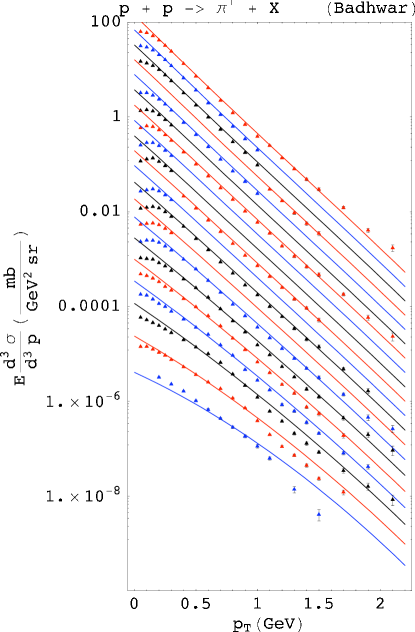
TABLE 4. Constants for the Mokhov parameterization.

Particle

$A$

$B$

$C$

$D$

$E$

$F$

$\;\;\pi^{+}$	60.1	1.9	0.18	0.3	12	2.7
$\;\;\pi^{-}$	51.2	2.6	0.17	0.3	12	2.7

II.2.5 Carey parameterization

The Carey carey parameterization, which only applies to $\pi^{-}$, is

$$E\frac{d^{3}\sigma}{d^{3}p}(\pi^{-})=N(p_{T}^{2}+0.86)^{-4.5}(1-x_{R})^{4}$$ (24)

where $N$ is an overall normalization fitted to be $N=13$ in reference blattnig and $x_{R}\equiv p/p_{\rm max}\approx 2p/\sqrt{s}$. The same value of $N$ is used in the present work. The Carey variables are $(p_{z},p_{T})$. To change to the variables $(x_{F},p_{T})$, we use $x_{R}=\sqrt{x_{F}^{2}+p_{T}^{2}/p_{\rm max}^{2}}$.

III COMPARISON TO DATA

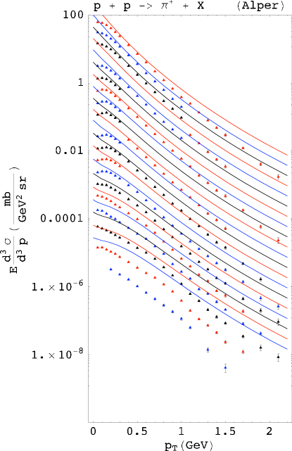
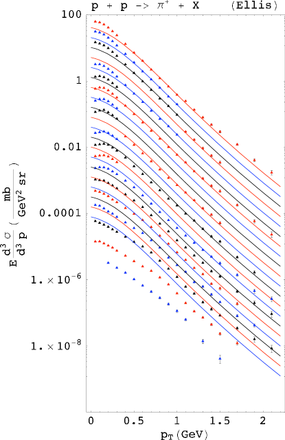
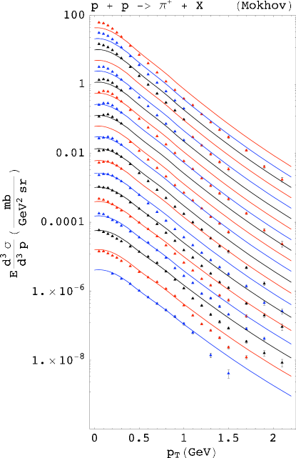
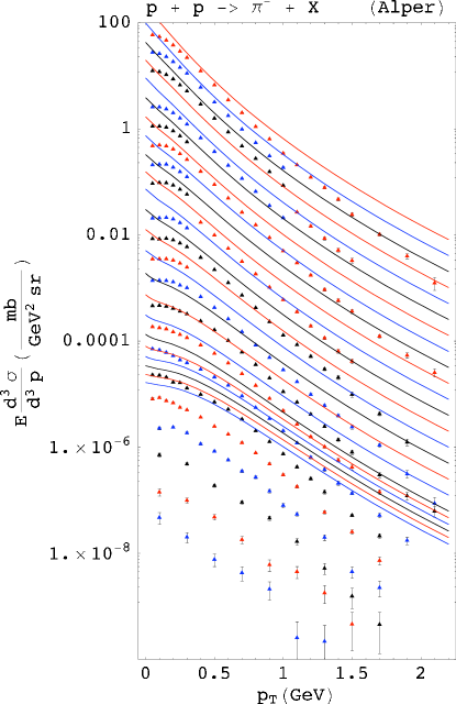
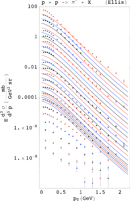
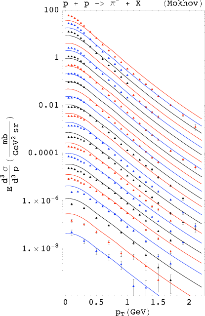
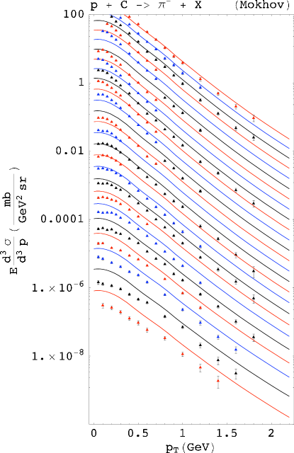
The above parameterizations are compared to the new experimental data in Figs. 1 - 13.

III.1 Comparison to $pp$ data

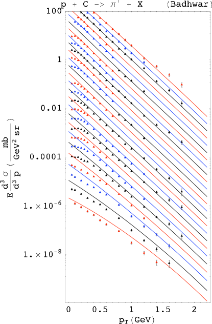
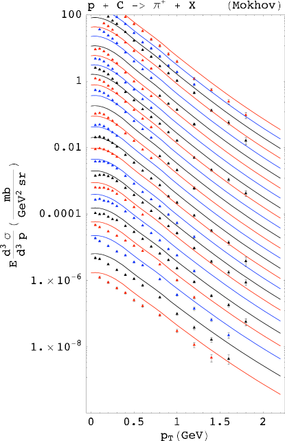
Positive pion production in $pp$ reactions is shown in Figs. 1 - 4. In agreement with the conclusions of the NA49 collaboration altpp , none of these arithmetic parameterizations is able to account for all the fine structure seen in the data. The Badhwar, Alper and Ellis parameterizations are unable to reproduce the shape of the differential cross section at low $p_{T}$. The Alper and Ellis parameterizations are unable to account for the data at larger values of $x_{F}$. However, on the positive side, the Mokhov parameterization (Fig. 4) does give a reasonable description of the shape at low $p_{T}$ and the Badhwar parameterization (Fig. 1) gives a reasonable fit to the data over all $x_{F}$ values for $p_{T}>0.3$ GeV. In general, the Alper and Ellis fits are not good, but the Badhwar and Mokhov fits are moderately good, but certainly not precise.

Figure 2: $\pi^{+}$ production in $pp$ collisions. Data from reference altpp is plotted against the parameterization of Alper alper . Values of $x_{F}$ and data and line multiplication are the same as Fig.1.

Figure 3: $\pi^{+}$ production in $pp$ collisions. Data from reference altpp is plotted against the parameterization of Ellis ellis . Values of $x_{F}$ and data and line multiplication are the same as Fig.1.

Figure 4: $\pi^{+}$ production in $pp$ collisions. Data from reference altpp is plotted against the parameterization of Mokhov mokhov . Values of $x_{F}$ and data and line multiplication are the same as Fig. 1.

Figure 5: $\pi^{-}$ production in $pp$ collisions. Data from reference altpp is plotted against the parameterization of Badhwar badhwar . The values of $x_{F}$ from top to bottom are 0.0, 0.01, 0.02, 0.025, 0.03, 0.04, 0.05, 0.06, 0.07, 0.075, 0.08, 0.1, 0.12, 0.15, 0.2, 0.25, 0.3, 0.35, 0.45, 0.55, 0.65, 0.75, 0.85. Following altpp , data and lines are multiplied successively by 0.5 up to $x_{F}=0.35$ and by 0.75 for $x_{F}\geq 0.45$ to allow for a better separation.

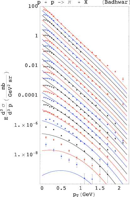
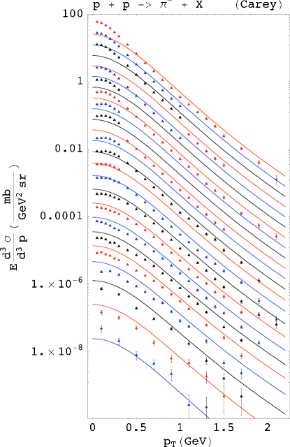
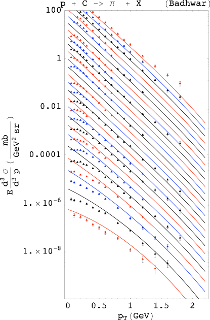
Negative pion production in $pp$ reactions is shown in Figs. 5 - 9. Again, in agreement with the conclusion of reference altpp , none of these arithmetic parameterizations is able to account for all the fine structure seen in the data. The conclusions are the same as for positive pions production, except that the Badhwar parameterization now fails for larger values of $x_{F}$. The Carey parameterization is reasonable except for small values of $x_{F}$ at low $p_{T}$. In general, the Alper and Ellis fits are not good, but the Badhwar, Mokhov and Carey fits are moderately good, but not precise.

Figure 6: $\pi^{-}$ production in $pp$ collisions. Data from reference altpp is plotted against the parameterization of Alper alper . Values of $x_{F}$ and data and line multiplication are the same as Fig.5.

Figure 7: $\pi^{-}$ production in $pp$ collisions. Data from reference altpp is plotted against the parameterization of Ellis ellis . Values of $x_{F}$ and data and line multiplication are the same as Fig.5.

Figure 8: $\pi^{-}$ production in $pp$ collisions. Data from reference altpp is plotted against the parameterization of Mohov mokhov . Values of $x_{F}$ and data and line multiplication are the same as Fig.5.

Figure 9: $\pi^{-}$ production in $pp$ collisions. Data from reference altpp is plotted against the parameterization of Carey carey . Values of $x_{F}$ and data and line multiplication are the same as Fig.5.

Figure 10: $\pi^{+}$ production in $pC$ collisions. Data from reference altpc is plotted against the parameterization of Badhwar badhwar multiplied by a best fit factor of $12^{0.9}$. The values of $x_{F}$ from top to bottom are -0.1, -0.075, -0.05, -0.04, -0.03, -0.025, -0.02, -0.01, 0.0, 0.01, 0.02, 0.025, 0.03, 0.04, 0.05, 0.06, 0.075, 0.1, 0.125, 0.15, 0.2, 0.25, 0.3, 0.4, 0.5. Following altpp , data and lines are multiplied successively by 0.5 to allow for a better separation.

III.2 Comparison to $pC$ data

Although the primary emphasis of this paper is on the $pp$ reactions, nevertheless it is of interest to see if the $pp$ parameterizations are able to scale to fit the new $pC$ data altpc , although a precise fit is not expected. We will only consider the parameterizations of Badhwar and Mokhov because they provided the best fits to the $pp$ data.

Figure 11: $\pi^{+}$ production in $pC$ collisions. Data from reference altpc is plotted against the parameterization of Mokhov mokhov multplied by a best fit factor of $12^{0.9}$. Values of $x_{F}$ and data and line multiplication are the same as Fig. 10.

One should note that in comparing to the $pC$ data we will assume the same cross section for proton-proton and proton-neutron scattering. However, as shown in the paper by Pawlowski and Szczurek pawlowski , this is known not to be true in general for the energy region of the new NA49 data. We justify our use of the same cross sections by noting the following. The data of Pawlowski and Szczurek pawlowski (see their Fig. 2), show that these cross sections are significantly different only for $x_{F}<-0.05$. For $x_{F}>-0.05$ the cross sections are very similar and in fact for $x_{F}>0$, Pawlowski and Szczurek pawlowski themselves state that $\sigma_{pp}^{\pi^{\pm}}\approx\sigma_{pn}^{\pi^{\pm}}$. In our comparisons, we show 25 different values of $x_{F}$. Only two of these, namely $x_{F}=-0.01$ and $x_{F}=-0.075$ are such that there is a significant difference between the proton-proton and proton-neutron cross section. For $\pi^{+}$ production the proton-proton cross section is about twice that of the proton-neutron cross section and vice-versa for $\pi^{-}$ pawlowski . This means that only for $x_{F}=-0.01$ and $x_{F}=-0.075$ our comparisons to data will be slightly worse for $\pi^{+}$ and slightly better for $\pi^{-}$. We now discuss various models.

Figure 12: $\pi^{-}$ production in $pC$ collisions. Data from reference altpc is plotted against the parameterization of Badhwar badhwar multplied by a best fit factor of $12^{0.9}$. Values of $x_{F}$ and data and line multiplication are the same as Fig. 10.

Figure 13: $\pi^{-}$ production in $pC$ collisions. Data from reference altpc is plotted against the parameterization of Mokhov mokhov multiplied by a best fit factor of $12^{0.9}$. Values of $x_{F}$ and data and line multiplication are the same as Fig. 10.

The wounded nucleon model was introduced by Bialas, Bleszynski and Czyz bialas . The number of wounded nucleons is simply the number of participants involved in the reaction. The main assumption is that the particle multiplicty is proportional to the number of wounded nucleons. Consider $pA$ reactions. The incident proton interacts with $\nu$ nucleons in the target nucleus soltz , which is some fraction of the total nucleon number $A$, and is determined from collision geometry and the hadron-nucleon cross section soltz . In a $pA$ reaction, the number of participants is $(1+\nu)$. Let $N_{pA}$ be the multiplicity of particles of interest produced in the $pA$ reaction, and let $N_{pp}$ be the particle multiplicity in the $pp$ reaction. For example this could be the number of pions produced in a reaction. The multiplicities are related by $N_{pA}=\frac{1}{2}(1+\nu)N_{pp}$ The $\frac{1}{2}$ factor is there because the “nucleon-nucleon interaction requires two wounded nucleons” navia . The following comes from reference navia . For a nucleus-nucleus collision let $A$ be the number of nucleons in the projectile and let $B$ be the number of nucleons in the target. Then navia $N_{AB}=\frac{1}{2}W_{AB}N_{pp}$ where $W_{AB}$ is the number of participant nucleons, i.e. the “number of nucleons that have interacted at least once” navia . This is given by navia $W_{AB}=A\frac{\sigma_{pB}}{\sigma_{AB}}+B\frac{\sigma_{pA}}{\sigma_{AB}}$ where $\sigma_{pA}$ and $\sigma_{pB}$ are the proton-nucleus inelastic cross sections and $\sigma_{AB}$ is the nucleus-nucleus cross section given in reference navia . If the projectile nucleus is actually a proton then $W_{pB}=\frac{\sigma_{pB}}{\sigma_{pB}}+B\frac{\sigma_{pp}}{\sigma_{pB}}=1+B\frac{\sigma_{pp}}{\sigma_{pB}}$ or $1+\nu=W_{pA}=1+A\frac{\sigma_{pp}}{\sigma_{pA}}$ showing that bialkowska $\nu=A\frac{\sigma_{pp}}{\sigma_{pA}}$. In $pA$ or $AA$ collisions then the particle multiplicity scales with the number of wounded nucleons, which is often calculated with Glauber theory huang .

Instead of wounded nucleon or participant scaling, one can have binary scaling. The total number of produced particles in nuclear collisions comes from both soft and hard processes. Soft processes should scale with the number of participants and hard processes should scale yin with the average number of binary nucleon-nucleon collisions denoted as $N_{\rm coll}$. Reference adcox contains a nice introduction to hard processes. For example, the PHENIX experiment adcox focuses on detecting large transverse momentum $p_{T}$ particles that arise from the early stages of relativistic heavy ion collisions. In the early stage nucleon-nucleon collisions cause jet production resulting from hard parton collisions. The jets subsequently decay into high momentum hadrons with $p_{T}\sim 2$ Gev adcox . The quark-gluon plasma (QGP) forms at a later time in the collision and the early scattered partons move through the QGP region leading to the phenomenon known as jet quenching which is signified by a “depletion in the yield of high $p_{T}$ hadrons” adcox . Observation of this jet quenching is therefore a “potential signature for QGP formation.”

The nuclear modification factor is a measure of nuclear effects and has been discussed by many authors blume ; szczurek ; yin ; adams ; adler ; adcox . For proton-nucleus reactions,

$$R_{pA}=\frac{Ed^{3}\sigma_{pA}/d^{3}p}{N_{\rm coll}\;Ed^{3}\sigma_{pp}/d^{3}p}$$ (25)

For nucleus-nucleus reactions,

$$R_{AB}=\frac{Ed^{3}\sigma_{AB}/d^{3}p}{N_{\rm coll}\;Ed^{3}\sigma_{NN}/d^{3}p}$$ (26)

where $NN$ refers to the nucleon-nucleon cross section. Instead of $d^{3}p$, other variables can be used such as $x_{F}$, $p_{T}$, rapidity, psuedorapidity, etc. The nuclear modification factor $R=1$ in the absence of nuclear effects, i.e. if the nuclear cross section is just an incoherent superposition of nucleon-nucleon collisions. For low $p_{T}<2$ GeV it has been found adcox that $R<1$ and this is due to the fact that the reactions scales with the number of participants (participant scaling), rather than the number of binary collisions adcox . For $p_{T}>2$ GeV “particle production in $pA$ collisions is enhanced compared to binary scaling” adcox , which is the Cronin effect.

Again consider participant scaling versus binary scaling. The nucleus-nucleus cross section could scale either as a function of the number of participants (often called wounded nucleons) or as a function of the number of binary nucleon-nucleon collisions. Binary scaling would indicate no collective effects whatsoever. However if there are some collective effects then these should manifest themselves by scaling with the number of participants. Obviously binary collisions are harder and lead to high $p_{T}$ processes such as jet production (from individual parton collisions) and heavy flavor production. Participant effects are generally softer processes at smaller $p_{T}$ such as soft hadron production, transverse energy flow and other collective phenomena. Both the number of participants $N_{\rm part}$ and the number of binary collisions $N_{\rm coll}$ is large for small impact parameter (central collisions) and drops off smoothly at larger impact parameters (peripheral collisions). Also we always have $N_{\rm coll}>N_{\rm part}$, because there can be many re-scatterings among the participants.

For a long time it has been known that energetic particle production in proton-nucleus collisions increases faster than the number of binary nucleon-nucleon collisions adler . In other words, particle production in nuclear collisions is enhanced compared to binary scaling adcox . This is known as the Cronin effect. Various physical mechanisms can contribute to the Cronin effect such as multiple parton scattering in the initial stage of the collision yin , Fermi motion szczurek , etc. Reference adler points out that the “the cause of the Cronin effect and its species dependence are not yet completely understood”, where species dependance refers to the fact that the size of the effect varies for different particles produced. A contribution from final state interactions is also possible adler . Reference adler provides a very nice summary of the Cronin effect. The $pA$ cross section is parameterized as adler ; vogt

$$E\frac{d^{3}\sigma}{d^{3}p}(p_{T},A)=E\frac{d^{3}\sigma}{d^{3}p}(p_{T},1)\;A^{\alpha(p_{T})}$$ (27)

where $\alpha>1$ indicates nuclear collective effects. Adler et al adler state that “the enhancement depends on the momentum and the type of particle produced, with protons and antiprotons exhibiting a much larger enhancment than pions and kaons at $p_{T}>2-3$ GeV.” They also point out that at $\sqrt{s}=27.4$ GeV, the enhancement reaches a maximum at $p_{T}=4.5$ GeV with $\alpha_{K}^{+}\sim\alpha_{\pi}^{+}=1.1$ and that at the same momentum $\alpha_{p}=1.3$ for protons adler .

In Figs. 10 - 13 we have simply multiplied the $pp$ parameterizations of Badhwar and Mokhov by a constant Cronin enhancement factor, $12^{\alpha}$, and compared them to the $pC$ data from NA49 altpc . In our previous $pp$ fits, the Badhwar parameterization worked best for high $p_{T}>0.5$ GeV and the Mokhov parameterization worked best for low $p_{T}<0.5$ GeV. Therefore we do not expect the Badhwar parameterization to fit low $p_{T}$ data for the $pC$ reaction and we do not expect the Mokhov parameterization to fit high $p_{T}$ data for the $pC$ reaction. We varied the value of $\alpha$ to find the best possible fit to the $pC$ data. Figs. 10 - 11 show the Badhwar fit to the high $p_{T}$ data with a best value of $\alpha=0.9$ and Figs. 12 - 13 show the Mokhov fit to the low $p_{T}$ data also with an independent best value of $\alpha=0.9$.

IV CONCLUSIONS

The NA49 collaboration altpp ; altpc has provided new precise data on pion production in $pp$ and $pC$ reactions at a beam momentum of 158 GeV. Although a precise fit is not expected, nevertheless it is of interest to compare currently available arithmetic parameterizations to the new data. Let us emphasize that we are not suggesting that arithmetic parameterizations are able to give a complete account of the new data et al altpp ; altpc . The numerical interpolation developed by the NA49 collaboration altpp ; altpc is far superior. The aim of this paper has rather been to see how well some parameterizations describe the data.

We conclude that the Alper and Ellis parameterizations do not fit the $pp$ data very well, and should not be used in this energy region. The Carey parameterization for $\pi^{-}$ works better but underpredicts the data at low $p_{T}$ for small values of $x_{F}$ and the predictions at high $p_{T}$ are only moderately good. The Badhwar parameterization for $\pi^{\pm}$ works well for high values of $p_{T}$, but does a poor job at low $p_{T}$, whereas the Mokhov parameterization is the other way around. It works best for low $p_{T}$ but not well for high $p_{T}$. Note also that the Badhwar parameterization for $\pi^{-}$ does not work well for large values of $x_{F}$, whereas the Mokhov parameterization works fine in this region. Regarding the $pp$ parameterizations, we conclude that for low $p_{T}<0.5$ GeV, it is best to use the Mokhov parameterization. For high $p_{T}>0.5$ GeV, is best to use the Badhwar parameterization, except for large values of $x_{F}>0.45$, where it is better to use Mokhov.

The Badhwar and Mokhov parameterizations gave good fits in certain $p_{T}$ ranges and we scaled them to the $pC$ data. In the Cronin effect, the scaling factor is $A^{\alpha(p_{T})}$. We found that the Badhwar parameterization gave the best fit for $\alpha\approx 0.9$, and the Mokhov parameterization also gave the best fit for $\alpha\approx 0.9$. As discussed above, the Badhwar parameterization works best for high $p_{T}$ and the Mokhov parameterization works best for low $p_{T}$. Therefore we conclude that the Cronin enhancement factor for the $pC$ reactions is $\alpha(p_{T})\approx 0.9$ in both the high $p_{T}>0.5$ GeV region and low $p_{T}<0.5$ GeV region. These results indicate the absence of nuclear collective effects adler for this $pC$ reaction altpc .

Acknowledgments. This work was supported by NASA grant NAG8-1901.

References

- (1) C. Alt et al. (NA49 Collaboration), Eur. Phys. J. C 45, 343 (2006).
- (2) C. Alt et al. (NA49 Collaboration), hep-ex/0606028..
- (3) R. Fernow, Introduction to Experimental Particle Physics (Cambridge University Press, New York, 1986); K. Kleinknecht, Detectors for Particle Radiation, 2nd ed., (Cambridge University Press, New York, 1998).
- (4) M. V. S. Rao and B. V. Sreekantan, Extensive Air Showers (World Scientific, Singapore, 1998).
- (5) T. K. Gaisser, Cosmic Rays and Particle Physics (Cambridge University Press, New York, 1990).
- (6) P. Sokolsky, Introduction to Ultrahigh Energy Cosmic Ray Physics (Addison-Wesley, Redwood City, CA, 1989).
- (7) M. S. Longair, High Energy Astrophysics, 2nd ed. (Cambridge University Press, New York, 1992)., Vol. 2.
- (8) J. W. Wilson, L. W. Townsend, W. S. Schimmerling, G. S. Khandelwal, F. Khan, J. E. Nealy, F. A. Cucinotta, L. C. Simonsen, J. L. Shinn and J. W. Norbury, Transport Methods and Interactions for Space Radiation, NASA Reference Publication No. 1257 (1991).
- (9) S. R. Blattnig, S. R. Swaminathan, A. T. Kruger, M. Ngom, and J. W. Norbury, Phys. Rev. D 62, 094030 (2000).
- (10) G. D. Badhwar, S. A. Stephens, and R.L. Golden, Phys. Rev. D 15, 820 (1977).
- (11) M. M. Kaufman Bernado, astro-ph/0504498.
- (12) E. Domingo-Santamaria and D. F. Torres, Astron. Astrophys. 444, 403 (2005).
- (13) T. Kamae, T. Abe, and T. Koi, Astrophys. J. 620, 244 (2005).
- (14) T. Kamae, N. Karlsson, T. Mizuno, T. Abe, and T. Koi, Astrophys. J. 647, 692 (2006).
- (15) S. R. Kelner, F. A. Aharonian, and V. V. Bugayov, Phys. Rev. D 74, 034018 (2006).
- (16) I. V. Moskalenko, astro-ph/0410241.
- (17) T. Prodanovic and B. D. Fields, astro-ph/0603618.
- (18) C. Blume, nucl-ex/0609022.
- (19) D. d’Enterria, Phys. Lett. B 596, 32 (2004).
- (20) D. d’Enterria, Eur. Phys. J. C 43, 295 (2005).
- (21) D. d’Enterria, J. Phys. G 31, S491 (2005).
- (22) R. Hagedorn, Relativistic Kinematics (W.A. Benjamin, Inc., New York, 1963).
- (23) B. P. Roe, Particle Physics at the new millenium (Springer-Verlag, New York, 1996).
- (24) P. D. B. Collins and A. D. Martin, Hadron Interactions (Adam Hilger Ltd., Bristol, 1984).
- (25) D. H. Perkins, Introduction to High Energy Physics, 2nd ed. (Addison-Wesley, Reading, Massachusetts, 1982).
- (26) J. Whitmore, Phys. Rep. 10, 273 (1974).
- (27) C. Y. Wong, Introduction to High-Energy Heavy-Ion Collisions (World Scientific, Singapore, 1994).
- (28) S. Nagamiya and M. Gyulassy, Adv. Nucl. Phys. 13, 201 (1984).
- (29) G. Giacomelli and M. Jacob, Phys. Rep. 55, 1 (1979).
- (30) M. J. Tannenbaum, Rep. Prog. Phys. 69, 2005 (2006).
- (31) W. Cassing, V. Metag, U. Mosel, and K. Nita, Phys. Rep. 188, 363 (1990).
- (32) B. Alper et al., Nucl. Phys. B 100, 237 (1975).
- (33) S. D. Ellis and R. Stroynowski, Rev. Mod. Phys. 49, 753 (1977).
- (34) N. V. Mokhov and S. I. Striganov, CP435, Workshop on the Front End of Muon Collider. 1998, pp. 453-459.
- (35) D. C. Carey et al., Phys. Rev. Lett. 33, 330 (1974).
- (36) P.Pawlowski and A.Szczurek, Phys. Rev. C 70 044908 (2004).
- (37) A. Bialas, A. Bleszynski, W. Czyz, Nucl. Phys. B 111, 461 (1976).
- (38) R. Soltz, J. Phys. G 27, 319 (2001).
- (39) C. E. Navia, H. V. Pinto, F. A. Pinto, R. H. Maldonado, and H. M. Portella, Phys. Rev. D 40, 2898 (1989).
- (40) H. Bialkowska, hep-ex/0609006.
- (41) D. W. Huang and E. Yen, Phys. Rev. C 40, 635 (1989).
- (42) Z. Yin, European Physical Journal (to be published).
- (43) K. Adcox et al. (PHENIX Collaboration), Phys. Rev. Lett. 88, 022301 (2002).
- (44) A. Szczurek and A. Budzanowski, nucl-th/0311025.
- (45) J. Adams et al. (STAR Collaboration), Phys. Rev. Lett. 97, 152302 (2006).
- (46) S. S. Adler et al. (PHENIX Collaboration), Phys. Rev. C 74, 024904 (2006).
- (47) R. Vogt, nucl-th/9903051.