,

Pion-photon Transition Distribution Amplitudes in the Spectral Quark Model

Abstract

The vector and axial pion-photon transition distribution amplitudes are analyzed in the Spectral Quark Model. We proceed by the evaluation of double distributions through the use of a manifestly covariant calculation based on the $\alpha$ representation of propagators. As a result polynomiality is incorporated and calculations become rather simple. Explicit formulas, holding at the low-energy quark-model scale, are obtained. The corresponding form factors for the anomalous decay $\pi^{0}\to\gamma\gamma^{\ast}$ and the radiative pion decays $\pi^{\pm}\to l^{\pm}\nu_{l}\gamma$ are also evaluated and confronted with the data.

Recently Pire and Szymanowski [1, 2] proposed generalizations of the parton distributions to the case where the initial and final states correspond to different particles. Such objects are termed transition distribution amplitudes (TDAs) and are relevant in the analysis of the virtual Compton scattering and other exclusive processes. For a recent review of a related topic of generalized parton distributions (GPDs) see, e.g., [3, 4, 5, 6, 7] and references therein. Of particular importance are the pion-photon vector and axial leading-twist TDAs, $V$ and $A$, which are the subject of this letter. A quark-model analysis of these objects has been undertaken by Tiburzi [8], where the relevant double distributions have been computed. Here we follow similar steps, however, instead of using parameterizations [9], we carry out an explicit analytical calculation all the way down using the Spectral Quark Model (SQM) [10]. This model possesses a regularization which allows for a uniform treatment of both anomalous and non-anomalous processes, essential in the study. It also encodes the vector-meson dominance and as a result leads to very successful phenomenology of numerous processes with pions, photons, or $\rho$-mesons. Below we obtain simple analytic expressions for $V$ and $A$ and the corresponding form factors, which hold at the low quark-model energy scale. Variants of chiral quark models have been used to obtain information on the pion structure function [11, 12], pion distribution amplitude [13, 14, 15, 16, 17], generalized parton distributions of the pion [18, 19, 20, 21, 22], and the photon and $\rho$ distribution amplitudes [23].

In this paper the considered TDAs are defined as [1]

$$\int\!\frac{dz^{-}}{2\pi}\,e^{ixp^{+}z^{-}}\!\langle\gamma(p^{\prime},\varepsilon)|\bar{\psi}(-\frac{z}{2})\gamma^{\mu}\frac{\tau^{a}}{2}{\psi}(\frac{z}{2})|\pi^{b}(p)\rangle\Big{|}_{\stackrel{{\scriptstyle z^{+}=0}}{{z_{T}=0}}}\!$$

$$=\!\frac{ie}{p^{+}f}\epsilon^{\mu\nu\alpha\beta}\varepsilon_{\nu}^{*}\,p_{\alpha}q_{\beta}V^{ab}(x,\zeta,t),$$

$$\int\!\frac{dz^{-}}{2\pi}\,e^{ixp^{+}z^{-}}\!\langle\gamma(p^{\prime},\varepsilon)|\bar{\psi}(-\frac{z}{2})\gamma^{\mu}\gamma_{5}\frac{\tau^{a}}{2}{\psi}(\frac{z}{2})|\pi^{b}(p)\rangle\Big{|}_{\stackrel{{\scriptstyle z^{+}=0}}{{z_{T}=0}}}\!$$

$$= \!\frac{e}{p^{+}f}(\varepsilon^{*}\cdot q)p^{\prime\mu}A^{ab}(x,\zeta,t)+\dots,$$ (3)

$$V^{ab}=\delta^{ab}V_{I=0}+i\epsilon^{ab3}V_{I=1},\;\;A^{ab}=\delta^{ab}A_{I=0}+i\epsilon^{ab3}A_{I=1},$$

where $\psi$ represents the iso-doublet quark field, $z$ is a light-cone coordinate ($z^{+}=0$, $z_{T}=0$), $p$ denotes the momentum of the pion, $f$ is the pion decay constant with $f=86$ MeV in the chiral limit, and the photon carries momentum $p^{\prime}=p+q$ and has polarization $\varepsilon$. Finally, in the asymmetric notation of GPDs we use $\zeta=q^{+}/p^{+}$ and $t=q^{2}$. We consider isovector quark bilinears. The isospin decomposition (3) follows from the fact that the photon couples to the quark through a combination of isoscalar and isovector coupling, i.e. the quark charge is $Q=1/(2N_{c})+\tau^{3}/2$. The presence of the gauge link operators $[-z/2,z/2]$ is understood in Eq. (Pion-photon Transition Distribution Amplitudes in the Spectral Quark Model,3) in order to guarantee gauge invariance of bilocal operators. For brevity, in Eq. (3) only the piece proportional to $(\varepsilon\cdot q)p^{\mu}$ is retained. The part proportional to $(\varepsilon\cdot q)q^{\mu}$, indicated by ellipses, corresponds to the pion pole term in the $t$-channel and is not relevant for the evaluation of the axial TDA (see [8] for a detailed discussion of the tensor structure including the pion pole term).

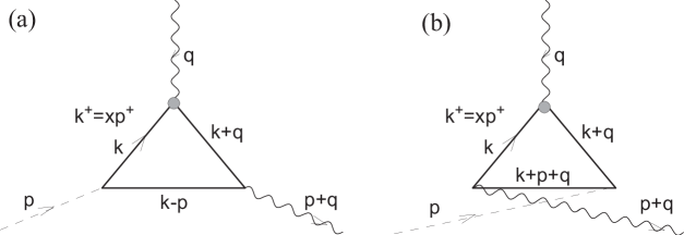
Figure 1: The direct (a) and crossed (b) Feynman diagrams for the quark-model evaluation of the pion-photon TDAs.

The quark-model evaluation of Eq. (Pion-photon Transition Distribution Amplitudes in the Spectral Quark Model,3) amounts to the calculation of the diagrams of Fig. 1, where the $+$ component of the momentum of the hit quark is constrained to the value $k^{+}=xP^{+}$. We denote $\omega$ as the constituent quark mass and use $\gamma_{5}\omega/f$ as the pion-quark coupling vertex as required by the Goldberger-Treiman relation at the quark level. We switch to the Euclidean momenta from now on. The $I=0$ and $I=1$ components are the following combinations of the direct and crossed diagrams of Fig. 1: $V_{I=0}=V+\bar{V}$, $V_{I=1}=N_{c}(V-\bar{V})$, where the bar indicates the crossed diagram, and similarly for $A$. Since the crossed contributions are related to the direct terms via a simple kinematic transformation, we first analyze the direct diagrams. For the vector TDA a simple algebra, involving the evaluation of the trace factor, yields

$$V(x,\zeta,t)=2\int\frac{d^{4}k}{(2\pi)^{4}}\frac{\delta(k\cdot n-x)\,\omega^{2}}{[{k^{2}+\omega^{2}}][{(k+q)^{2}+\omega^{2}}][{(k-p)^{2}+\omega^{2}}]},$$ (4)

where $n^{2}=0$, $p\cdot n=1$, and $q\cdot n=-\zeta$. Our basic technique makes use of the $\alpha$ representation for the scalar propagators, which allows for a covariant treatment of the $\delta$ function. Thus,

$$V(x,\zeta,t) = 2\,\omega^{2}\int\frac{d^{4}k}{(2\pi)^{4}}\int\frac{d\lambda}{2\pi}e^{i\lambda(k\cdot n-x)}$$

$$\times \int_{0}^{\infty}d\alpha\int_{0}^{\infty}d\beta\int_{0}^{\infty}d\gamma\,e^{-\alpha(k^{2}+\omega^{2})-\beta((k+q)^{2}+\omega^{2})-\gamma((k-p)^{2}+\omega^{2})}.$$

Next, we introduce the variables $s=\alpha+\beta+\gamma$, $y={\beta}/{s}$, and $z={\gamma}/{s}$, shift the momentum to $k=k^{\prime}+zp-yq+i\lambda n/(2s)$, and then perform the Gaussian integral over $k$. Note that since $\alpha,\beta,\gamma\geq 0$, we get $0\leq y,z\leq 1$ and also $y+z\leq 1$. As a result,

$$V\!=\!\frac{\omega^{2}}{8\pi^{2}}\!\int_{0}^{1}\!\!dy\!\int_{0}^{1}\!\!dz\theta(1\!-y\!-z)\!\int_{0}^{\infty}\!ds\delta\left(x\!-\!z\!-y\zeta\right)e^{-s[\omega^{2}+y(1-y)q^{2}+z(1-z)p^{2}+2yzp\cdot q]}$$ (6)

$$= \frac{1}{8\pi^{2}}\int_{0}^{1}dy\!\int_{0}^{1}dz\delta\left(x\!-\!z\!-\!y\zeta\right)D(z,y),$$

where

$$D(z,y) = \frac{\theta(1-y-z)\,\omega^{2}}{\omega^{2}+y(1-y)q^{2}+z(1-z)p^{2}+2yzp\cdot q},$$ (7)

is the double distribution for the vector TDA. With our Euclidean vectors $p^{2}=-m_{\pi}^{2}$, $q^{2}=-t$, and $2p\cdot q=m_{\pi}^{2}+t$ for the real photon. Equation (7) agrees with the result of Ref. [8]. Note that our use of the $\alpha$-representation has led to a direct evaluation of TDAs from the Feynman diagrams. This is a very simple alternative to the more involved expansion in moments, typically done in similar studies.

For TDAs the variable $\zeta$ cannot be assumed to be positive, as the crossing symmetry does not relate initial and final states, unlike for GPDs. In general we have $-1\leq\zeta\leq 1$. Next, we perform the $z$ integration, which sets $z=x-y\zeta$. For the case $\zeta\geq 0$ this gives

$$V(x,\zeta,t)=\frac{1}{8\pi^{2}}\left(\theta[x(\zeta\!-\!x)]\!\!\int_{0}^{\frac{x}{\zeta}}\!\!+\theta[(x\!-\!\zeta)(1\!-\!x)]\!\!\int_{0}^{\frac{1-x}{1-\zeta}}\right)\!dyD(x\!-y\zeta,y),\;(\zeta\geq 0),$$ (8)

with the first term having the support $x\in[0,\zeta]$, and the second $x\in[\zeta,1]$. For the case $\zeta<0$ we obtain

$$V(x,\zeta,t)=\frac{1}{8\pi^{2}}\left(\theta[x(\zeta-x)]\!\!\int_{\frac{x}{\zeta}}^{\frac{1-x}{1-\zeta}}\!\!+\theta[x(1-x)]\!\!\int_{0}^{\frac{1-x}{1-\zeta}}\right)dyD(x-y\zeta,y),\;(\zeta<0),$$ (9)

with the support $x\in[\zeta,0)$ for the first term and $x\in[0,1]$ for the second term. Thus the support is correct. As expected, the function $V$ is continuous in the $x$ variable, with the derivative $dV/dx$ discontinuous at the points $x=0,\zeta,1$.

The contribution from the crossed diagram is formally obtained from the direct diagram with the replacement and $p\to-p-q$. Replacing correspondingly $x\to\zeta-x$ and performing the München transformation: $z\to z$, $y\to 1-y-z$, yields the result ${\bar{V}}(x,\zeta,t)=V(\zeta-x,\zeta,t)$. The support of the crossed diagram reflects the support of the direct diagram. For the case $\zeta\geq 0$ it is $x\in[-1+\zeta,\zeta]$, while for $\zeta<0$ we have $x\in[-1+\zeta,0]$.

The evaluation of the axial TDA proceeds analogously, with the trace yielding an additional proportionality factor $(2k+q)\cdot\varepsilon$ as compared to the vector TDA in Eq. (4). The result is

$$A(x,\zeta,t)=\frac{1}{8\pi^{2}}\int_{0}^{1}dy\int_{0}^{1}dz\delta\left(x-z-y\zeta\right)(2y+2z-1)D(z,y).$$ (10)

In the present case ${\bar{A}}(x,\zeta,t)=-A(\zeta-x,\zeta,t)$, with the minus coming from the trace factor.

Expressing the TDAs through the double distributions has the known advantage of an automatic verification of the polynomiality conditions which ultimately correspond to proper implementation of the Lorentz invariance. Polynomiality is manifest from this form, as the moments $\int dxV(x,\zeta,t)x^{n}$ involve integrals with the factor $(z+y\zeta)^{n}$ and result in a polynomial in $\zeta$ of order $n$. We end these general considerations by writing down the double distributions in the so called symmetric variables, $\alpha$, and $\beta$ (not to be confused with the previously introduced Feynman parameters), defined as $y=(1+\alpha-\beta)/2$, $z=\beta$. For the vector case we find

$$D(\alpha,\beta)=\frac{\theta(1-|\alpha|-\beta)\theta(\beta)\omega^{2}}{\omega^{2}+[1-(\alpha-\beta)^{2}]q^{2}/4+\beta(1-\beta)p^{2}+(1+\alpha-\beta)\beta p\cdot q},$$ (11)

while for the axial case we find $(\alpha+\beta)D(\alpha,\beta)$, in full agreement with Ref. [8]. The theta functions provide the standard integration limits $\int_{0}^{1}d\beta\int_{-1+|\beta|}^{1-|\beta|}d\alpha$.

The general expressions presented above are formal, as quark models require regularization. The choice of a finite regularization is far from trivial, as requirements of the Lorentz and gauge invariance, as well as preservation of chiral Ward identities and in particular anomalies (crucial in the present study) impose severe and tight constraints. An elegant way of imposing a regularization which obeys these requirements is achieved in the Spectral Quark Model (SQM) [10]. In this model, developed in the spirit of the early work of Efimov and Ivanov [24], the quark mass $\omega$ is treated as a spectral parameter of a generalized Lehmann representation, which is integrated along a suitably chosen complex contour $C$. The chirally symmetric effective action constructed in Ref. [10] reads

$$\Gamma[U,v,a]=-iN_{c}\int_{C}d\omega\rho(\omega){\rm Tr}\log\left(i\hbox to0.0pt{\hbox to5.30904pt{\hfil/\hfil}\hss}\partial-\omega U^{5}-\left(\hbox to0.0pt{\hbox to5.20601pt{\hfil/\hfil}\hss}v+\hbox to0.0pt{\hbox to5.28589pt{\hfil/\hfil}\hss}a\gamma_{5}\right)\right),$$ (12)

where the trace for a bilocal (Dirac- and flavor-matrix valued) operator $A(x,x^{\prime})$ is given by ${\rm Tr}A=\int d^{4}x\,{\rm tr}\langle A(x,x)\rangle$ with ${\rm tr}$ denoting the Dirac trace and $\langle\,\rangle$ the flavor trace. The matrix $U^{5}=e^{i\gamma_{5}\mathchoice{\mbox{\boldmath$\displaystyle\tau$}}{\mbox{\boldmath$\textstyle\tau$}}{\mbox{\boldmath$\scriptstyle\tau$}}{\mbox{\boldmath$\scriptscriptstyle\tau$}}\cdot\mathchoice{\mbox{\boldmath$\displaystyle\pi$}}{\mbox{\boldmath$\textstyle\pi$}}{\mbox{\boldmath$\scriptstyle\pi$}}{\mbox{\boldmath$\scriptscriptstyle\pi$}}/f}=\frac{1}{2}(1+\gamma_{5})U+\frac{1}{2}(1-\gamma_{5})U^{\dagger}$, while $U=e^{{i}\mathchoice{\mbox{\boldmath$\displaystyle\pi$}}{\mbox{\boldmath$\textstyle\pi$}}{\mbox{\boldmath$\scriptstyle\pi$}}{\mbox{\boldmath$\scriptscriptstyle\pi$}}\cdot\mathchoice{\mbox{\boldmath$\displaystyle\tau$}}{\mbox{\boldmath$\textstyle\tau$}}{\mbox{\boldmath$\scriptstyle\tau$}}{\mbox{\boldmath$\scriptscriptstyle\tau$}}/f}$ is the flavor matrix representing the pseudoscalar pions in the nonlinear representation. The symbols $v^{\mu}$ and $a^{\mu}$ represent external vector and axial currents. In Eq. (12) the spectral density $\rho(\omega)$ acts as a regulator. Actually, the expressions for one-quark-loop observables in SQM are obtained from the preceding expressions by integrating over $\omega$ with the spectral density $\rho(\omega)$. For a generic observable $F$ we have

$$F_{\rm SQM}=\int_{C}d\omega\rho(\omega)F(\omega),$$ (13)

where $F(\omega)$ is the quark-model result with the quark mass set to $\omega$. In the meson-dominance version of SQM [10] we have

$$\rho(\omega) = \rho_{V}(\omega)+\rho_{S}(\omega),$$ (14)

$$\rho_{V}(\omega) = \frac{1}{2\pi i}\frac{1}{\omega}\frac{1}{(1-4\omega^{2}/M_{V}^{2})^{5/2}},\;\rho_{S}(\omega)=-\frac{1}{2\pi iN_{c}M_{S}^{4}}\frac{48\pi^{2}\langle\bar{q}q\rangle}{(1-4\omega^{2}/M_{S}^{2})^{5/2}},$$

where $M_{S}=M_{V}=m_{\rho}$ is the $\rho$-meson mass [25]. The contour $C$ for the spectral integration over $\omega$ and other details are given in Ref [10]. SQM generates the monopole pion electromagnetic form factor [10]. Interestingly, the model has the feature of the analytic quark confinement, i.e. the quark propagator has no poles, only cuts, in the complex momentum plane. Moreover, the evaluation of low-energy matrix elements in SQM is very simple and leads to numerous results reported in Ref. [10], in particular for the pion light-cone wave function, the pion structure function, the generalized parton distributions of the pion [21], low energy chiral Lagrangeans [25] and the photon, and $\rho$-meson structure functions [23].

Let us assume for simplicity from now on the chiral limit, $p^{2}=0$, and the real photon, $(p+q)^{2}=0$. The evaluation of the spectral integral is straightforward using the results of Ref. [25]. Then the double distribution for the vector TDA in SQM assumes the simple form

$${D}_{\rm SQM}(z,y)=\int_{C}d\omega\rho(\omega){D}(z,y)=\frac{\theta(1-y-z)}{\left(1-\frac{4y(1-y-z)t}{M_{V}^{2}}\right)^{5/2}}.$$ (15)

Remarkably, completely analytic expressions for the TDAs follow, fulfilling all a priori Lorentz, chiral and gauge invariance constraints. To our knowledge this is the first explicit calculation of TDAs in a regularized chiral quark model, and we list the results in some detail as their form may guide the used parameterizations of TDAs. We only show the results for the case $\zeta\geq 0$, as for $\zeta\leq 0$ they have a similar character. We find for the vector TDA

$$V_{\rm SQM}(x,\zeta,t) = \frac{M_{V}^{2}}{48\pi^{2}}\left(\theta[x(\zeta-x)]\left(\chi_{1}+\frac{\chi_{2}}{2}\right)+\theta[(1-x)(x-\zeta)]\chi_{2}\right),$$ (16)

where

$$\chi_{2}=\frac{2(x-1)\left[3(\zeta-1)M_{V}^{2}+t(x-1)^{2}\right]}{\left[(\zeta-1)M_{V}^{2}+t(x-1)^{2}\right]^{2}},$$ (17)

$$\chi_{1}=\frac{(x(\zeta-2)+\zeta)\left(3M_{V}^{2}(\zeta-1)\zeta^{2}+t\left(\left(\zeta^{2}+8\zeta-8\right)x^{2}+2(4-5\zeta)\zeta x+\zeta^{2}\right)\right)}{\left((\zeta-1)M_{V}^{2}+t(x-1)^{2}\right)^{2}\left({\zeta^{2}+\frac{4tx(x-\zeta)}{M_{V}^{2}}}\right)^{3/2}}.$$

Some special values are

$$V_{\rm SQM}(0,\zeta,t) = V_{\rm SQM}(1,\zeta,t)=0,\;\;V_{\rm SQM}(\zeta,\zeta,t)=\frac{M_{V}^{2}\left(3M_{V}^{2}+t(\zeta-1)\right)}{24\pi^{2}\left(M_{V}^{2}+t(\zeta-1)\right)^{2}},$$

$$V_{\rm SQM}(x,\zeta,0) = \frac{1}{8\pi^{2}}\left(\theta[x(\zeta-x)]\frac{x}{\zeta}+\theta[(1-x)(x-\zeta)]\frac{1-x}{1-\zeta}\right),$$

$$V_{\rm SQM}(x,0,t) = \frac{M_{V}^{2}\left(3M_{V}^{2}-t(1-x)^{2}\right)(1-x)}{24\pi^{2}\left(M_{V}^{2}-t(1-x)^{2}\right)^{2}}.$$ (18)

The functions $8\pi^{2}V_{\rm SQM}(x,\zeta,t)$ are shown at the top of Fig. 2 for two values of $t$ and for several values of $\zeta$, both positive and negative. The integration over $x$ produces the $\zeta$-independent (as required by polynomiality) form factors,

$$\int dxV^{I=0}_{\rm SQM}(x,\zeta;t)\!=\!\int dx\left(V_{\rm SQM}\!+\!{\bar{V}}_{\rm SQM}\right)=\frac{M_{V}^{2}}{24\pi^{2}}\left(\frac{2}{M_{V}^{2}-t}-\frac{\log\left(1-\frac{t}{M_{V}^{2}}\right)}{t}\right).$$

$$\int dxV^{I=1}_{\rm SQM}(x,\zeta;t)=\int dxN_{c}\left(V_{\rm SQM}-{\bar{V}}_{\rm SQM}\right)=0.$$ (19)

The isoscalar form factor is related to the pion-photon transition form factor,

$$F_{\pi\gamma\gamma^{\ast}}(t)=\frac{2}{f}\int dxV^{I=0}=\frac{1}{4\pi^{2}f}\left(1+\frac{5t}{6M_{V}^{2}}+\frac{7t^{2}}{9M_{V}^{7}}\dots\right),$$ (20)

where the factor of 2 comes from the fact, that either of the photons can be isoscalar. We read out the corresponding rms radius to be $\langle r^{2}\rangle^{1/2}_{\pi\gamma\gamma^{\ast}}=\sqrt{5}/M_{V}=0.57{\rm fm}$ for $M_{V}=770{\rm MeV}$. Equivalently, one may use the slope parameter $b_{\pi}=\frac{d}{dt}F_{\pi^{0}\gamma\gamma^{\ast}}(t)/F_{\pi^{0}\gamma\gamma^{\ast}}(t)\Big{|}_{t=0}$. SQM gives $b_{\pi}=5/(6M_{V}^{2})=1.4~{}{\rm GeV}^{-2}$, in very reasonable agreement with the experimental values quoted by the PDG [26]: $b_{\pi}=(1.79\pm 0.14\pm 14){\rm GeV}^{-2}$ originally reported by the CELLO collaboration [27], $b_{\pi}=(1.4\pm 1.3\pm 2.6){\rm GeV}^{-2}$ from Ref. [28], or $b_{\pi}=(1.4\pm 0.8\pm 1.4){\rm GeV}^{-2}$ given in [29].

The vector form factor is also related to the $F_{V}$ form factor appearing in the radiative pion decays, $\pi^{\pm}\to l^{\pm}\nu_{l}\gamma$ (for a review see e.g. [30] and references therein). With the assumption of CVC it is related to the the isoscalar form factor in the following way:

$$F_{V}(t)=\frac{\sqrt{2}m_{\pi}}{f}\int dxV^{I=0}=\frac{\sqrt{2}m_{\pi}}{8\pi^{2}f}\left(1+\frac{5t}{6M_{V}^{2}}+\dots\right).$$ (21)

The premultiplying factors follow the assumed conventions. The value at $t=0$ (for $f=93$ MeV) is $F_{V}(0)\simeq 0.026$, as listed in [26]. The experimental data fall one standard deviation below this CVC prediction, with $F_{V}(0)=0.017\pm 0.008$ [26].

Figure 2: Top: vector TDA $8\pi^{2}V_{\rm SQM}(x,\zeta,t)$ for $t=0$ (left) and $t=-0.4$ GeV (right) plotted as functions of $x$ for several values of $\zeta$: $-1$, $-2/3$, $-1/3$, $0$, $1/3$, $2/3$, and $1$. The value of $\zeta$ can be inferred from the position of the cusp for $\zeta>0$ or from the support for $\zeta<0$. Bottom: the same for the axial TDA $8\pi^{2}V_{\rm SQM}(x,\zeta,t)$. The vector curves are normalized to $1/2$, and the axial curves to $1/6$. The presented calculation is made in the Spectral Quark Model with $M_{V}=0.77$ GeV in chiral limit and for the real photon.

For the axial TDA the corresponding expressions are (for $\zeta\geq 0$)

$$A_{\rm SQM}(x,\zeta,t) = \frac{M_{V}^{2}}{48\pi^{2}}\left(\theta[x(\zeta-x)]\chi_{3}+\theta[(1-x)(x-\zeta)]x\chi_{2}\right),$$ (22)

where $\chi_{2}$ is given by Eq. (Pion-photon Transition Distribution Amplitudes in the Spectral Quark Model) and

$$\chi_{3}=\frac{(\zeta-1)^{2}M_{V}^{4}+t(x-1)(5x-2)(\zeta-1)M_{V}^{2}+t^{2}(x-1)^{3}(2x-1)}{t\left(t(x-1)^{2}+(\zeta-1)M_{V}^{2}\right)^{2}}+$$

$$\frac{1}{t\left(M_{V}^{2}+\frac{4tx(x-\zeta)}{\zeta^{2}}\right)^{3/2}\left(t(x-1)^{2}+(\zeta-1)M_{V}^{2}\right)^{2}}$$ (23)

$$\times\left[-(\zeta-1)^{2}\zeta^{3}M_{V}^{4}+t(\zeta-1)\zeta^{2}\left((\zeta-6)x^{2}+7\zeta x-2\zeta\right)M_{V}^{2}+\right.$$

$$\left.t^{2}\left(16x^{4}-24(x+1)\zeta x^{3}+6(x(x+6)+1)\zeta^{2}x^{2}-(5x(x(x+3)-1)+1)\zeta^{3}\right)\right].$$

The special values are

$$A_{\rm SQM}(0,\zeta,t)=A_{\rm SQM}(1,\zeta,t)=0,$$

$$A_{\rm SQM}(\zeta,\zeta,t)=\frac{\zeta M_{V}^{2}\left(3M_{V}^{2}+t(\zeta-1)\right)}{24\pi^{2}\left(M_{V}^{2}+t(\zeta-1)\right)^{2}}=\zeta V_{\rm SQM}(\zeta,\zeta,t),$$

$$A_{\rm SQM}(x,\zeta,0)=\frac{1}{8\pi^{2}}\left(\theta[x(\zeta\!-\!x)]\frac{x(\zeta x+x-\zeta)}{\zeta^{2}}+\theta[(1\!-\!x)(x\!-\!\zeta)]\frac{x(1\!-\!x)}{(1\!-\!\zeta)}\right),$$

$$A_{\rm SQM}(x,0,t)=\frac{M_{V}^{2}\left(3M_{V}^{2}-t(1-x)^{2}\right)(1-x)x}{24\pi^{2}\left(M_{V}^{2}-t(1-x)^{2}\right)^{2}}=xV_{\rm SQM}(x,0,t).$$ (24)

The form factors are

$$\int dxA^{I=0}_{\rm SQM}(x,\zeta,t)=\int dx\left(A_{\rm SQM}+{\bar{A}}_{\rm SQM}\right)=0,$$

$$\int dxA^{I=1}_{\rm SQM}(x,\zeta,t)\!=\!\int dxN_{c}\left(A_{\rm SQM}\!-\!{\bar{A}}_{\rm SQM}\right)=-\frac{M_{V}^{2}N_{c}}{24\pi^{2}}\frac{\log\left(1-\frac{t}{M_{V}^{2}}\right)}{t}.$$ (25)

The bottom part of Fig. 2 displays the function $8\pi^{2}A_{\rm SQM}(x,\zeta,t)$.

The axial TDA is related to the axial-vector form factor measured in the radiative pion decays $\pi^{\pm}\to l^{\pm}\nu_{l}\gamma$ via integration over the $x$ variable,

$$F_{A}(t)=\frac{\sqrt{2}m_{\pi}}{f}\int dxA^{I=1}(x,\zeta,t)=\frac{\sqrt{2}N_{c}m_{\pi}}{24\pi^{2}f}\left(1+\frac{t}{2M_{V}^{2}}+\frac{t^{2}}{3M_{V}^{4}}+\dots\right),$$ (26)

where the premultiplying factors are the same as in Eq. (21). The value at $t=0$ is $F_{A}(0)=F_{V}(0)\simeq 0.026$, which is a factor of 2 larger than the experimental number $F_{A}(0)=0.0115\pm 0.0005$ [26]. The same conclusions were reached in Ref. [8]. The predicted ratio $F_{A}(0)/F_{V}(0)=1$ compares to the experimental number of $F_{A}(0)/F_{V}(0)=0.7^{+0.6}_{-0.2}$ within one standard deviation. The $t$-dependence of the form factors is presented in Fig. 3. We note long tails due to a $\log(-t)/t$ behavior at large $t$. The axial form factor (dashed line) lies above the vector form factor (solid line), which in turn lies above the monopole vector-meson dominance form factor, drawn as reference (dotted line).

It is interesting to analyze our results in the light of Chiral Perturbation Theory in the large-$N_{c}$ limit [31], where $F_{A}(0)=4(L_{10}+L_{9})\sqrt{2}m_{\pi}/f_{\pi}=0.012\pm 0.008$ for $L_{9}=(6.9\pm 0.7)\cdot 10^{-3}$ and $L_{10}=(-5.5\pm 0.7)\cdot 10^{-3}$ (in fact the values of the low-energy constants $L_{9}$ and $L_{10}$ are determined from the pion electromagnetic form factor and the radiative pion decays). In the large-$N_{c}$ limit one imposes QCD-motivated short-distance constraints regarding the asymptotic falloff both for the difference of two-point vector minus axial correlators (the Weinberg sum rules) as well as the axial and electromagnetic form factors at large $t$ (see, e.g., [32]). In the single resonance approximation (SRA) one gets the same value for $F_{V}$ as above and since $L_{9}^{\rm SRA}=-4L_{10}^{\rm SRA}/3=f^{2}/2M_{V}^{2}$ a ratio $F_{A}(0)/F_{V}(0)\sim 1/2\sqrt{2}=0.35$ which produces a significantly lower value for the axial form factor, $F_{A}^{\rm SRA}(0)\sim 0.01$. In SQM one has $L_{9}^{\rm SQM}=-2L_{10}^{\rm SQM}=N_{c}/(48\pi^{2})$ [25] and hence $F_{A}^{\rm SQM}(0)=0.026$ in agreement with Eq. (26). The mismatch in the $L_{10}/L_{9}$ ratio in SQM and SRA stems from the absence of an explicit axial meson contribution in SQM which induces the violation of the second Weinberg sum rule pointed out previously [10] and generating a $F_{A}(0)$ about twice the experimental number. This feature is common to all known local quark models. The SQM axial radius and the large-$N_{c}$ SRA result coincide, $\langle r^{2}\rangle_{A}=3/M_{V}^{2}$, although at large $t$ SRA yields $F_{A}(t)\sim 1/t$ which is slightly more convergent than our result (25), which contains an additional $\log(-t)$. It would be interesting to pursue the present calculation to the nonlocal chiral quark models where both Weinberg sum rules are known to hold [33]. Finally, the large $t$-behavior is subjected to the QCD logarithmic radiative corrections.

Figure 3: Form factors $F_{\pi\to\gamma\gamma^{\ast}}(t)/F_{\pi\to\gamma\gamma^{\ast}}(0)$ (solid line) and $F_{A}(t)/F_{A}(0)$ (dashed line). The dotted line shows as reference the electromagnetic form factor which in SQM is a monopole $F_{\pi}^{\rm em}(t)=M_{V}^{2}/(M_{V}^{2}-t)$.

Actually, the results obtained above hold at a low energy scale of the quark model. In Ref. [11] an estimate of this scale based on the momentum sum rule has been given. For the present model or other local models, such as the Nambu–Jona-Lasinio model, the scale turns out to be very low, around 320 MeV. An independent estimate based on the pion light-cone distribution amplitude results in a very similar estimate [17]. For that reason, evolution is crucial for the case of DAs of PDFs, and undoubtedly will also be important for the present case of TDAs as well as the vector and axial form factors at large momenta. The results obtained so far simply provide the initial conditions for the QCD evolution, which at the leading order can be made with the usual ERBL equations [34, 35]. A detailed study of the evolution issues will be presented elsewhere.

In conclusion, we have presented an explicit quark-model study of the vector and axial leading-twist pion-photon TDAs. The results are analytic, which allows us to gain insight into the possible forms of non-perturbatively generated TDAs. Such predictions for TDAs or GPDs are scarce, and frequently one only makes guesses subject to the constraints coming from form factors, polynomiality, etc. Our method conforms to the Lorentz and gauge invariance, preserves the chiral Ward-Takahashi identities as well as satisfies anomalies, crucial in the study of the VAA processes. Since we proceed via the double distributions, our TDAs automatically satisfy the polynomiality constraints. The used technique of calculation, which takes advantage of the $\alpha$-representation of propagators and thus is manifestly covariant, makes a direct use of the Feynman diagrams and produces the results in a few straightforward steps. No expansion in terms of moments is necessary. This technique is applicable also in other calculations of this kind: PDFs, GPDs, as well as for other models, including the non-local models, where the quark mass depends on the virtuality. Our results correspond to a low-energy quark-model scale. After suitable QCD evolution the obtained results may be used in the studies of the virtual Compton scattering and other exclusive processes involving pions, photons, and the weak gauge bosons.

We thank Brian Tiburzi for helpful e-mail exchanges and for pointing out a mistake in one of our formulas.

References

[1]
B. Pire and L. Szymanowski, Phys. Rev.D71 (2005) 111501.
[2]
B. Pire and L. Szymanowski, Phys. Lett.B622 (2005) 83–92.
[3]
X.-D. Ji, J. Phys.G24 (1998)
1181–1205.
[4]
K. J. Golec-Biernat and A. D. Martin, Phys. Rev.D59 (1999) 014029.
[5]
K. Goeke, M. V. Polyakov, and M. Vanderhaeghen, Prog. Part. Nucl. Phys.47 (2001)
401–515.
[6]
M. Diehl, Phys. Rept.388
(2003) 41–277.
[7]
A. V. Belitsky and A. V. Radyushkin, Phys. Rept.418 (2005)
1–387.
[8]
B. C. Tiburzi, Phys. Rev.D72 (2005) 094001.
[9]
J. P. Lansberg, B. Pire, and L. Szymanowski, Phys. Rev.D73 (2006) 074014.
[10]
E. Ruiz Arriola and W. Broniowski, Phys. Rev.D67 (2003) 074021.
[11]
R. M. Davidson and E. Ruiz Arriola, Phys. Lett.B348 (1995)
163–169.
[12]
T. Frederico and G. A. Miller, Phys. Rev.D50 (1994)
210–216.
[13]
V. Y. Petrov, M. V. Polyakov, R. Ruskov, C. Weiss, and K. Goeke, Phys.
Rev.D59 (1999) 114018.
[14]
I. V. Anikin, A. E. Dorokhov, and L. Tomio, Phys. Atom. Nucl.64 (2001)
1329–1336.
[15]
M. Praszalowicz and A. Rostworowski, Phys. Rev.D64 (2001) 074003.
[16]
A. E. Dorokhov, JETP Lett.77 (2003) 63–67.
[17]
E. Ruiz Arriola and W. Broniowski, Phys. Rev.D66 (2002) 094016.
[18]
M. V. Polyakov and C. Weiss, Phys. Rev.D60 (1999) 114017.
[19]
S. Noguera, L. Theussl, and V. Vento, Eur. Phys. J.A20 (2004)
483–498.
[20]
B. C. Tiburzi and G. A. Miller, Phys. Rev.D67 (2003) 013010.
[21]
W. Broniowski and E. Ruiz Arriola, Phys. Lett.B574 (2003) 57–64.
[22]
S. Noguera and V. Vento, Eur. Phys. J.A28 (2006) 227–236.
[23]
A. E. Dorokhov, W. Broniowski, and E. Ruiz Arriola, Phys.
Rev.D74 (2006) 054023.
[24]
G. V. Efimov and M. A. Ivanov, Quark Confinement Model of Hadrons.
IOP, Bristol, 1993.
[25]
E. Megias, E. Ruiz Arriola, L. L. Salcedo, and W. Broniowski, Phys. Rev.D70 (2004) 034031.
[26]Particle Data Group Collaboration, S. Eidelman et al., Phys. Lett.B592 (2004)
1.
[27]CELLO Collaboration, H. J. Behrend et al., Z. Phys.C49 (1991)
401–410.
[28]
F. Farzanpay et al., Phys. Lett.B278 (1992)
413–418.
[29]SINDRUM-I Collaboration, R. Meijer Drees et al., Phys. Rev.D45
(1992)
1439–1447.
[30]
D. A. Bryman, P. Depommier and C. Leroy,
Phys. Rept. 88 (1982) 151.
[31]
G. Ecker, J. Gasser, H. Leutwyler, A. Pich, and E. de Rafael, Phys. Lett.B223 (1989)
425.
[32]
A. Pich, in The Phenomenology of Large QCD, Tempe, Arizona, Jan. 2002, p. 239,
ed. R. Lebed, World Scientific, Singapore, 2002.
hep-ph/0205030.
[33]
W. Broniowski, in Hadron Physics: Effective theories of low-energy QCD,
Coimbra, Portugal, Sept. 1999, AIP Conference Proceedings, vol. 508, p. 380,
eds. A. H. Blin, B. Hiller, M. C. Ruivo, C. A. Sousa and E. van Beveren,
AIP, Melville, New York, 1999,
hep-ph/9911204.
[34]
A. V. Efremov and A. V. Radyushkin, Phys. Lett.B94 (1980)
245–250.
[35]
G. P. Lepage and S. J. Brodsky, Phys. Rev.D22 (1980)
2157.