QCD at small ${\boldsymbol{x}}$ and nucleus-nucleus collisions

Abstract

At large collision energy $\sqrt{s}$ and relatively low momentum transfer $Q$, one expects a new regime of Quantum Chromo-Dynamics (QCD) known as “saturation”. This kinematical range is characterized by a very large occupation number for gluons inside hadrons and nuclei; this is the region where higher twist contributions are as large as the leading twist contributions incorporated in collinear factorization. In this talk, I discuss the onset of and dynamics in the saturation regime, some of its experimental signatures, and its implications for the early stages of Heavy Ion Collisions.

1 Hadrons and nuclei at high energy

A nucleon at low energy can be seen as made of three valence quarks, constantly interacting via gluon exchanges and virtual fluctuations at all space-time scales smaller than the size of the nucleon itself. In an interaction process with a probe, only those fluctuations which are longer lived/larger than the resolution of the probe are actually relevant. In addition, interaction processes at low energy are made very complicated by the fact that the constituents of the nucleon can interact during the time seen by the probe. When one boosts the nucleon to a higher energy, all its internal time scales are dilated, which simplifies the interaction process with the probe: the interactions among the constituents of the nucleon now occur over much larger time-scales, and therefore the probe sees only a collection of free constituents. Moreover, the life-time of the quantum fluctuations is also time dilated, and thus the number of gluons taking part to the interaction process increases with the collision energy. Simultaneously, the fluctuations that were already important at the lower energy are now evolving so slowly that they can be considered static over the time-scale seen by the external probe.

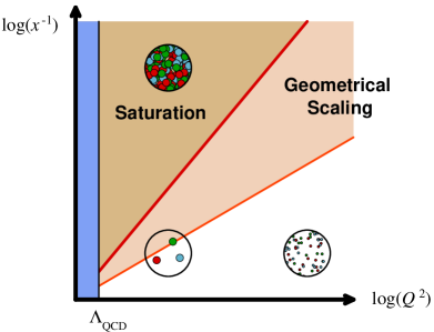
Figure 1: Saturation domain in the $(Q^{2},x)$ plane. We have also represented the larger domain where geometrical scaling occurs.

However, this growth with energy of the number of gluons in the wave-function of a nucleon (or nucleus) cannot continue indefinitely. Indeed, it would imply that nucleon-nucleon cross-sections grow faster than what is allowed by Froissart’s unitarity bound. In fact, an important aspect of the physics is missing in the above picture: gluons can recombine when their occupation number is large, a process known as gluon saturation [1]. To quantify when this new phenomenon occurs, one must compare the number of gluons per unit of transverse area, $\rho\sim xG(x,Q^{2})/\pi R^{2}$, and the cross-section for recombination, $\sigma\sim\alpha_{s}/Q^{2}$. Saturation occurs when $1\lesssim\rho\sigma$, or equivalently $Q^{2}\leq Q_{s}^{2}(x)$, where $Q_{s}(x)=\alpha_{s}xG(x,Q_{s}^{2})/\pi R^{2}$ is known as the saturation momentum. The equation $Q^{2}=Q_{s}^{2}(x)$ delineates the border of the saturation domain, indicated in figure 1. Phenomenologically, $Q_{s}^{2}$ varies like $A^{1/3}x^{-0.3}$ with the nucleus atomic number $A$ and the momentum fraction $x$.

2 Color Glass Condensate

The Color Glass Condensate (CGC) is a description of the nature of the saturated nuclear matter, in which a saturation scale emerges naturally. In the CGC description, the fast partons (large $x$) are described as static color sources – represented by a density $\rho({\boldsymbol{x}}_{\perp})$ in the transverse plane – that act as external sources. Conversely, the slow partons (low $x$), dominated by gluons, are described by the usual dynamical gauge fields $A^{\mu}$. Such a separation of the degrees of freedom was first proposed in the McLerran-Venugopalan model [2]. In order to make this description complete, one needs to specify the distribution $W_{{}_{Y}}[\rho]$ for the hard sources in a projectile that has evolved up to the rapidity $Y\equiv\ln(1/x)$. This distribution is in principle non-perturbative, but its evolution with rapidity $Y$ is controlled by an evolution equation that can be derived in perturbation theory [3],

$$\frac{\partial W_{{}_{Y}}[\rho]}{\partial Y}={\cal H}[\rho]\;W_{{}_{Y}}[\rho]\;,$$ (1)

known as the JIMWLK equation. This functional evolution equation can be seen as an extension of the BFKL equation [5] that incorporates the effect of gluon recombination. It has a very useful mean field approximation: the Balitsky-Kovchegov equation [4]. These evolution equations are presently known at leading logarithmic accuracy, but several recent works have extended them in order to include the Next-to-Leading Order corrections that come from the running of the strong coupling constant [6]. Another direction actively pursued is aimed at including “pomeron loops” in this description (see [7] for recent advances). Pomeron loops can be seen as fluctuations that are important in the region when the gluon occupation number is low, and may affect crucially the rapidity evolution of scattering amplitudes since it is controlled by the tail of the gluon distribution.

3 Experimental evidence of saturation

         

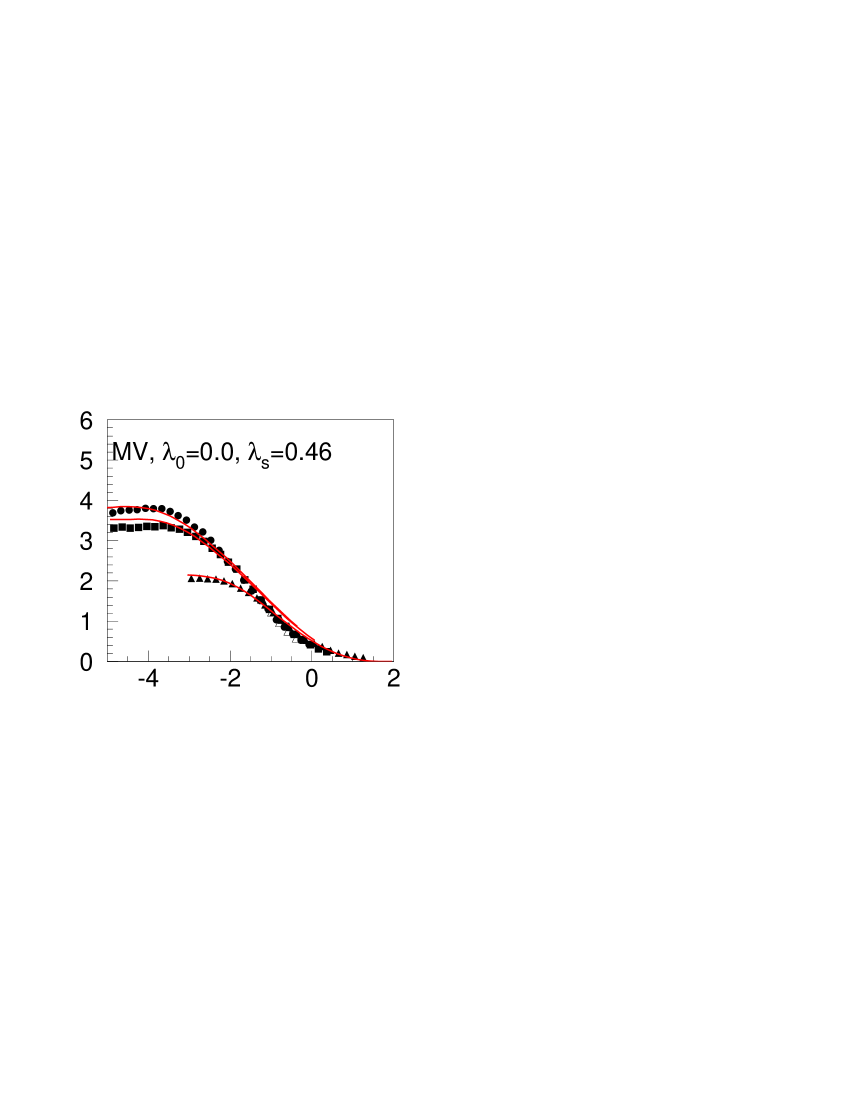
Figure 2: Left: geometrical scaling in the $\gamma^{*}$-proton cross-section at HERA. Right: Limiting fragmentation in RHIC data.

The first evidence of saturation comes from the “geometrical scaling” observed in Deep Inelastic Scattering at HERA [8]. There, the measured $\gamma^{*}p$ cross-section at $x\leq 0.01$ – which in principle depends on both variables $x$ and $Q^{2}$ – was found to depend only on the combination $\tau\equiv\ln(Q^{2}/Q_{s}^{2}(x))$ with $Q_{s}^{2}\propto x^{-0.3}$ (see the left panel of figure 2). Such a scaling is a direct consequence of the behavior of solutions of the evolution equation for the distribution of sources in the target proton, and the value of the exponent $0.3$ can be accounted for from a careful analysis of these solutions [9]. Going beyond this simple scaling, saturation physics leads to very good fits to a broad set of data from HERA and RHIC [10].

Another experimental result which is suggestive of saturation is the so-called “limiting fragmentation” (right panel of figure 2). By shifting the rapidity axis by the beam rapidity, one can see that the rapidity distribution for produced particles at collisions of various energies tend to some universal curve in the fragmentation region [11]. In the CGC framework, this property follows naturally from the unitarization of scattering amplitudes in the dense target, and the approximate Bjorken scaling in the fragmenting nucleus. The limiting curve then appears to be a reflection of the parton distribution at large $x$ in the fragmenting nucleus [12].

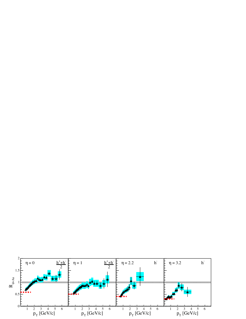
Figure 3: Forward suppression observed by BRAHMS.

The observation of the suppression of hadron spectra at rather large $p_{\perp}$ and forward rapidity in deuteron-gold collisions at RHIC [13] (see figure 3 for BRAHMS results) provides further information on the onset of saturation. The fact that the nuclear modification factor $R_{\rm dA}$ is larger than unity at mid rapidity is believed to be an effect of multiple scatterings (Cronin effect), and the suppression of this ratio at forward rapidities is a consequence of the shadowing that builds up via the evolution in $Y$ [14].

4 Initial particle production in nucleus-nucleus collisions

In order to use the CGC framework to describe the collision of two nucleons or nuclei, one needs two color sources $\rho_{1,2}$, representing respectively the two projectiles, that couple to the gauge fields (see [15] for a detailed discussion on this) via the following current,

$$J^{\mu}\equiv\delta^{\mu+}\delta(x^{-})\rho_{1}({\boldsymbol{x}}_{\perp})+\delta^{\mu-}\delta(x^{+})\rho_{2}({\boldsymbol{x}}_{\perp})\;.$$ (2)

As illustrated in figure 4, the description of Heavy Ion Collisions is usually split into several stages, each of them being described by different theoretical tools. It is expected that perturbation theory is appropriate for the very early stages, during which the constituents of the incoming nuclei are released and particles are initially produced.

     

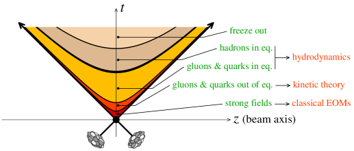
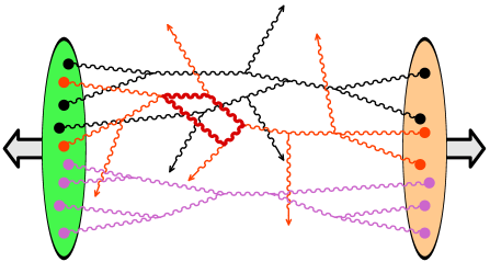
Figure 4: Left: the successive stages of a heavy ion collision. Right: typical diagram contributing to gluon production in the collision of two nuclei at high energy.

However, in a typical central heavy ion collision at high energy, 99% of the produced particles have a transverse momentum below 2 GeV – i.e. below the saturation momentum. In this region, collinear factorization breaks down, and it is believed that the CGC framework is more appropriate for describing the initial particle production.

In the saturation regime, the sources $\rho_{1,2}$ are typically of order of $1/g$, which alters the power counting for gluon production: adding an extra source to a given diagram does not change its order, implying that the color sources $\rho_{1,2}$ should be included to all orders. A typical diagram contributing to gluon production from these sources is illustrated in the right panel of figure 4. In general, there are several disconnected subdiagrams, including some that do not produce any gluon (vacuum diagrams) [17].

4.1 Gluon production at Leading Order

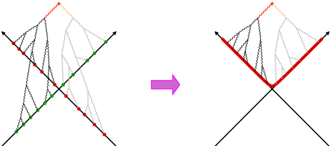
Figure 5: Gluon multiplicity at leading order. Left: tree retarded diagrams contributing to the gluon spectrum. The color sources are represented by red and green dots. Right: reformulation as an initial value problem on the light-cone.

At leading order [16], one must sum all the tree diagrams, with an arbitrary number of color sources – in general a very complicated task. However, for the inclusive gluon spectrum, this can be done from the classical solution of Yang-Mills equations with retarded boundary conditions. The retarded nature of the boundary conditions leads to an important simplification: one can reformulate the problem as an initial value problem where one specifies the fields and their first time derivatives just above the light-cone (and these initial conditions can be obtained analytically). This classical solution of the equation of motion is a sum of tree diagrams with retarded propagators, as illustrated in figure 5. An important feature of the classical solution of Yang-Mills equations is its invariance under boosts in the longitudinal solution, which implies that the field has only zero modes with respect to the rapidity variable $\eta$.

4.2 Gluon production at Next to Leading Order

In order to make the foundations of this description more robust, it is important to study loop corrections. One reason for doing so is to check the factorization of the leading logarithms of $1/x$ in the evolution of the distribution of sources $W[\rho_{1,2}]$, which is necessary for the internal consistency of this framework. Another motivation comes from the recent observation that the LO boost invariant solution is unstable against rapidity dependent perturbations [19] – and loop corrections are a natural origin for such perturbations.

Although the LO calculation of the gluon spectrum is non-perturbative since it requires to solve the Yang-Mills equation to all orders in the sources $\rho_{1,2}$, it turns out that one can express the 1-loop contributions as a perturbation of the initial value problem encountered at LO. There are two contributions, illustrated in figure 6. The NLO correction can be obtained by the action of some analytically calculable operator on the LO contribution, seen as a functional of the fields and canonical momenta on the light-cone [20],

$$\delta N_{{}_{NLO}}=\Big{[}\!\!\!\!\int\limits_{{\boldsymbol{x}}\in{\rm light-cone}}\!\!\!\!\!\!\!\!\delta{\cal A}({\boldsymbol{x}}){\boldsymbol{T}}_{\boldsymbol{x}}+\frac{1}{2}\!\!\!\!\int\limits_{{\boldsymbol{x}},{\boldsymbol{y}}\in{\rm light-cone}}\!\!\!\!\!\!\!\!{\boldsymbol{\Sigma}}({\boldsymbol{x}},{\boldsymbol{y}}){\boldsymbol{T}}_{\boldsymbol{x}}{\boldsymbol{T}}_{\boldsymbol{y}}\Big{]}\;N_{{}_{LO}}[{\cal A}_{\rm in}[\rho_{1},\rho_{2}]]\;.\;$$ (3)

In this formula, $\delta{\cal A}({\boldsymbol{x}})$ and ${\boldsymbol{\Sigma}}({\boldsymbol{x}},{\boldsymbol{y}})$ are respectively the 1-point and 2-point functions represented in green in figure 6 – they are in principle calculable analytically. ${\boldsymbol{T}}_{\boldsymbol{x}}$ is the generator of shifts of the initial condition at point ${\boldsymbol{x}}$ on the light-cone for the solution of Yang-Mills equations, i.e. a functional derivative $\delta/\delta{\cal A}_{\rm in}({\boldsymbol{x}})$.

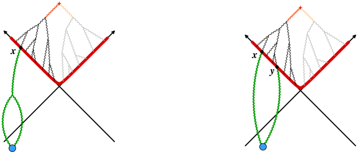
Figure 6: The two contributions to the gluon multiplicity at NLO.

Eq. (3) is sufficient to discuss the structure of singularities that arise at 1-loop :

• the coefficients $\delta{\cal A}$ and ${\boldsymbol{\Sigma}}$ are infinite, due to divergences in integrations over rapidity [21].

• the quantity ${\boldsymbol{T}}_{\boldsymbol{x}}\,{\cal A}(\tau,{\boldsymbol{y}})$ diverges when the time $\tau$ goes to infinity. This is due to the instability of the boost invariant classical solution found in [19].

The first type of divergences is related to the evolution with rapidity of the distributions $W[\rho_{1,2}]$. For the CGC framework to be consistent, one should be able to absorb these divergences in the rapidity dependence of $W[\rho_{1,2}]$ – a statement very similar in spirit to the factorization of collinear divergences in conventional perturbative QCD. Another way to state the same problem is to set fictitious boundaries in rapidity, $Y_{0}$ and $Y_{0}^{\prime}$, between the observable (here the number operator) and the color sources. Now, all integrations over rapidity in the observable are over the finite range $[Y_{0}^{\prime},Y_{0}]$, and thus lead to a finite result. Thus, $\delta{\cal A}$ and ${\boldsymbol{\Sigma}}$ become finite, but $Y_{0}$ and $Y_{0}^{\prime}$ dependent. Naturally, the distributions of color sources, $W[\rho_{1,2}]$, must now be evolved from the beam rapidities to $Y_{0}$ and $Y_{0}^{\prime}$ respectively. The factorization alluded to before is equivalent to the requirement that the $Y_{0}$ and $Y_{0}^{\prime}$ dependence cancel between the 1-loop correction to the observable and the rapidity evolution of the distributions of sources. For this cancellation to happen, one will need to establish the following relation for these divergent terms [20] :

$$\Big{[}\delta N_{{}_{NLO}}\Big{]}_{{\rm divergent}\atop{\rm coefficients}}=\Big{[}(Y_{0}-Y){\cal H}^{\dagger}[\rho_{1}]+(Y-Y_{0}^{\prime}){\cal H}^{\dagger}[\rho_{2}]\Big{]}\;N_{{}_{LO}}[{\cal A}_{\rm in}]\;,\;$$ (4)

where ${\cal H}[\rho]$ is the same Hamiltonian as in the JIMWLK evolution equation.

The second type of problem is due to an instability of the boost invariant solution of the classical Yang-Mills equations [19]. After resummation of these divergences to all orders, the operator acting on $N_{{}_{LO}}$ in Eq. (3) will be replaced by some functional $Z[{\boldsymbol{T}}_{\boldsymbol{x}}]$. Formally, one can perform a “Fourier transform” of this functional by introducing some auxiliary field $a({\boldsymbol{x}})$ on the light-cone, and then rewrite the contribution of the resummed unstable modes as

$$\Big{[}\delta N_{{}_{NLO}}\Big{]}_{{\rm unstable}\atop{\rm modes}} = \int\big{[}Da({\boldsymbol{x}})\big{]}\;\widetilde{Z}[a]\;\exp\Big{\{}i\int_{\boldsymbol{x}}a({\boldsymbol{x}}){\boldsymbol{T}}_{\boldsymbol{x}}\Big{\}}\;N_{{}_{LO}}[{\cal A}_{\rm in}]$$ (5)

$$= \int\big{[}Da({\boldsymbol{x}})\big{]}\;\widetilde{Z}[a]\;N_{{}_{LO}}[{\cal A}_{\rm in}+a]\;.$$

In other words, resumming the unstable modes can be done by solving the classical Yang-Mills equations with a fluctuation $a({\boldsymbol{x}})$ superimposed to the boost invariant initial condition ${\cal A}_{\rm in}$, with a distribution $\widetilde{Z}[a]$. This is the formal justification for the fluctuations added to the initial conditions in [19]. By a completely different approach [22], it appears that the functional $\widetilde{Z}[a]$ is a Gaussian, suggesting that the resummation of the unstable modes is simply an exponentiation.

5 Conclusions

QCD at small $x$, and in particular gluon saturation, has become an important aspect of hadronic collisions at RHIC and LHC energies. In nucleus-nucleus collisions, the CGC is the appropriate framework to study the early stages of the collision, because most of the particles are produced from low $x$ gluons. It seems now technically feasible to compute the 1-loop corrections to the gluon spectrum, and to resum their diverging terms. Doing so would allow one to prove for the CGC framework factorization results that are crucial for the overall consistency of this approach.

Acknowledgements :  Important parts of this talk are based on work done in collaboration with K. Fukushima, T. Lappi, L. McLerran and R. Venugopalan.

References

References

- [1] Gribov L V, Levin E M, Ryskin M G, Phys. Rep. 100, (1983) 1; Mueller A H, Qiu J-W, Nucl. Phys.B268, (1986) 427; Blaizot J P, Mueller A H, Nucl. Phys.B289, (1987) 847.
- [2] McLerran L D, Venugopalan R, Phys. Rev.D49, (1994) 2233; ibid. 3352; ibid. D50, (1994) 2225.
- [3] Jalilian-Marian J, Kovner A, McLerran L D, Weigert H, Phys. Rev. D55, (1997) 5414; Jalilian-Marian J, Kovner A, Leonidov A, Weigert H, Nucl. Phys. B504, (1997) 415; Phys. Rev. D59, (1999) 014014; ibid. 034007; ibid. Erratum 099903; Iancu E, Leonidov A, McLerran L D, Nucl. Phys. A692, (2001) 583; Phys. Lett. B510, (2001) 133; Ferreiro E, Iancu E, Leonidov A, McLerran L D, Nucl. Phys. A703, (2002) 489.
- [4] Balitsky I, Nucl. Phys. B463, (1996) 99; Kovchegov Yu, Phys. Rev. D61, (2000) 074018.
- [5] Balitsky I, Lipatov L N, Sov. J. Nucl. Phys. 28, (1978) 822; Kuraev E A, Lipatov L N, Fadin V S, Sov. Phys. JETP 45, (1977) 199.
- [6] Gardi E, Kuokkanen J, Rummukainen K, Weigert H, hep-ph/0609087; Kovchegov Yu, Weigert H, hep-ph/0609090; hep-ph/0612071; Balitsky I, Phys. Rev. D75, (2007) 014001.
- [7] Hatta Y, Iancu E, Marquet C, Soyez G, Triantafyllopoulos D N, Nucl. Phys. A773, (2006) 95; Iancu E, Marquet C, Soyez G, Nucl. Phys. A780, (2006) 52; Blaizot J-P, Iancu E, Triantafyllopoulos D N, hep-ph/0606253; Iancu E, de Santana Amaral J T, Soyez G, Triantafyllopoulos D N, hep-ph/0611105; Shoshi A I, Xiao B-W, hep-ph/0605282; Bondarenko S, Motyka L, Mueller A H, Shoshi A I, Xiao B-W, hep-ph/0609213; Kozlov M, Shoshi A I, Xiao B-W, hep-ph/0612053; Kozlov M, Levin E, Nucl. Phys. A779, (2006) 142; Kozlov M, Levin E, Prygarin A, hep-ph/0606260; Levin E, hep-ph/0608043; Kozlov M, Levin E, Khachatryan V, Miller J, hep-ph/0610084; Kovner A, Lublinsky M, Nucl. Phys. A779, (2006) 220.
- [8] H1 collaboration, Acta Phys. Polon. B33, (2002) 2841; ZEUS collaboration, Phys. Lett. B345, (1995) 576; Stasto A M, Golec-Biernat K, Kwiecinski J, Phys. Rev. Lett. 86, (2001) 596; Gelis F, Peschanski R, Schoeffel L, Soyez G, hep-ph/0610435.
- [9] Iancu E, Itakura K, McLerran L, Nucl. Phys. A708, (2002) 327; Munier S, Peschanski R, Phys. Rev. Lett. 91, (2003) 232001; Triantafyllopoulos D N, Nucl. Phys. B648 (2003) 293.
- [10] Iancu E, Itakura K, Munier S, Phys. Lett. B590, (2004) 199; Kowalski H, Motyka L, Watt G, Phys. Rev. D74, (2006) 074016; Forshaw J R, Sandapen R, Shaw G, JHEP 0611, (2006) 025; Dumitru A, Hayashigaki A, Jalilian-Marian J, Nucl. Phys. A770, (2006) 57; Goncalves V P, Kugeratski M S, Machado M V T, Navarra F S, Phys. Lett. B643, (2006) 273.
- [11] Bearden I G et al, Phys. Lett. B523, (2001) 227; Phys. Rev. Lett. 88, (2002) 20230; Back B B et al, Phys. Rev. Lett. 91, (2003) 052303; nucl-ex/0509034; Adams J et al, Phys. Rev. Lett. 95, (2005) 062301; Phys. Rev. C73, (2006) 034906.
- [12] Jalilian-Marian J, Phys. Rev. C70, (2004) 027902; Bialas A, Jeżabek M, Phys. Lett. B590, (2004) 233; Gelis F, Stasto A M, Venugopalan R, Eur. Phys. J C48, (2006) 489.
- [13] Arsene I et al., Phys. Rev. Lett. 93 (2004) 242303; Adams J et al., Phys. Rev. Lett. 97, (2006) 152302.
- [14] Kharzeev D, Levin E, McLerran L D, Phys. Lett. B561, (2003) 93; Baier R , Kovner A , Wiedemann U A, Phys. Rev. D68 (2003), 054009; Gelis F, Jalilian-Marian J, Phys. Rev. D67, (2003) 074019; Kharzeev D, Kovchegov Yu, Tuchin K, Phys. Rev. D68, (2003) 094013; Phys. Lett. B599, (2004) 23; Albacete J L, Armesto N, Kovner A, Salgado C A, Wiedemann U A, Phys. Rev. Lett. 92, (2004) 082001; Iancu E, Itakura K, Triantafyllopoulos D N, Nucl. Phys. A742, (2004) 182; Blaizot J-P, Gelis F, Venugopalan R, Nucl. Phys. A743, (2004) 13; Baier R, Mehtar-Tani Y, Schiff D, Nucl. Phys. A764, (2006) 515.
- [15] Hatta Y, Nucl. Phys. A781, (2007) 104.
- [16] Krasnitz A, Venugopalan R, Nucl. Phys. B557, (1999) 237; Phys. Rev. Lett. 84, (2000) 4309; ibid. 86, (2001) 1717; Krasnitz A, Nara Y, Venugopalan R, Nucl. Phys. A727, (2003) 427; Phys. Rev. Lett. 87, (2001) 192302; Lappi T, Phys. Rev. C67, (2003) 054903.
- [17] Gelis F, Venugopalan R, Nucl. Phys. A776, (2006) 135, ibid. A779, (2006) 177.
- [18] Gelis F, Kajantie K, Lappi T, Phys. Rev. C71, (2005) 024904; Phys. Rev. Lett. 96, (2006) 032304.
- [19] Romatschke P, Venugopalan R, Phys. Rev. Lett. 96, (2006) 062302; Eur. Phys. J. A29, (2006) 71; Phys. Rev. D74, (2006) 045011; Venugopalan R, these proceedings.
- [20] Gelis F, Lappi T, Venugopalan R, work in progress.
- [21] Lappi L, McLerran L D, Nucl. Phys. A772, (2006) 200.
- [22] Fukushima K, Gelis F, McLerran L D, hep-ph/0610416.