First correction to JIMWLK evolution from the classical equations of motion

Abstract

We calculate some ${\cal O}(\alpha_{s}^{2})$ corrections to the JIMWLK kernel in the framework of the light-cone wave function approach to the high energy limit of QCD. The contributions that we consider originate from higher order corrections in the strong coupling and in the density of the projectile to the solution of the classical Yang-Mills equations of motion that determine the Weizsäcker-Williams fields of the projectile. We study the structure of these corrections in the dipole limit, showing that they are subleading in the limit of large number of colours $N$, and that they cannot be fully recast in the form of dipole degrees of freedom.

1 Introduction: the wave function formalism and JIMWLK

The study of high gluon density QCD, pioneered in the MV model [1], has become a fashionable subject both due to its theoretical relevance and to eventual applications to small-$x$ DIS or high-energy nuclear collisions (see the review [2]). The main outcome of these studies was the JIMWLK equation which controls the evolution of the colour distribution of a hadron with increasing energy. In the last 3 years, the limitations of such evolution equation have become apparent in the form of the discussion of fluctuations and pomeron loops, see the reviews [3]. In all available schemes, a separation of scales is considered between fast partons which act as sources for the classical dynamics of the soft, slow glue. Considering gluon radiation and the arbitrariness of the fast-slow separation led to a renormalization group equation, the JIMWLK equation. A powerful framework to derive this equation, in which its limitations become apparent, is the wave function approach (WFA) [4] which we briefly introduce in this Section, see full details in [4, 5].

In the WFA the evolution is introduced in the wave function of the projectile scattering off a hadronic target. This wave function is the superposition of fast gluons with $k^{+}>\Lambda$. The scattering matrix with the target is the superposition of independent scattering matrices $S^{ab}$. Then, an average over target configurations is taken,

$$\Sigma_{Y}[S]=\langle\Psi^{i}(Y)|\Psi^{f}(Y)\rangle,\qquad\langle\Sigma\rangle=\int dS\,\Sigma[S]\,W_{Y}[S],$$ (1)

with $W_{Y}[S]$ the probability density for the target to have a certain configuration of the fields. After a boost $Y\to Y+\delta Y$, the wave functions become

$$|\Psi^{f}(Y+\delta Y)\rangle=\left\{1-\frac{1}{2}\delta Y\int d^{2}z\,b_{i}^{a}(z,S\rho)b_{i}^{a}(z,S\rho)\right.$$ (2)

$$+\left.i\int d^{2}z\,b_{i}^{a}(z,S\rho)\int_{(1-\delta Y)\Lambda}^{\Lambda}\frac{dk^{+}}{\sqrt{\pi}|k^{+}|^{1/2}}S^{ab}(z)a_{i}^{{}^{\dagger}b}(k^{+},z)\right\}|\Psi^{f}(Y)\rangle,$$

with $S^{ab}\to\delta^{ab}$ for $|\Psi^{i}(Y+\delta Y)\rangle$, $\rho$ the projectile density operator and $b_{i}^{a}$ the Weizsäcker-Williams fields of the projectile (WW) determined from the classical Yang-Mills equations of motion (EOMs), in which the hard gluons enter as an external source.

The resulting evolution equation is $\delta\Sigma[S]/\delta Y=\chi\,\Sigma[S]$, with the kernel given by

$$\chi=-\frac{1}{2\pi}\int_{z}\,\left[b_{i}^{a}(J_{L})b_{i}^{a}(J_{L})+b_{i}^{a}(J_{R})b_{i}^{a}(J_{R})-2S^{ba}(z)b_{i}^{a}(J_{L})b_{i}^{b}(J_{R})\right],$$ (3)

where $b_{i}^{a}$ depends on $z$ and $J_{L(R)}$ are left (right) colour rotation operators, whose action in the dipole model limit, with the projectile composed of colour dipoles [4], is illustrated in Figure 1. With the EOMs solved at lowest order in $g\rho$ in the $A^{+}=0$ gauge [1],

$$b^{a}_{i}(z)=g\left(b^{a}_{i1}(z)+g^{2}\,b^{a}_{i2}(z)+\mathcal{O}(g^{4})\right),\qquad b^{a}_{i1}(z)=\int\!{d^{2}x\over 2\pi}\,\left(\partial_{i}X\right)\rho^{a}(z),$$ (4)

with $\partial_{i}X\equiv\partial^{z}_{i}\ln\left(|z-x|\lambda\right)$, the JIMWLK evolution equation is obtained [4].

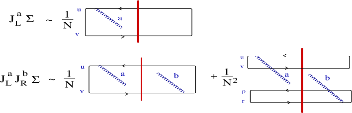
Figure 1: Diagrammatic representation of $J_{L}^{a}\Sigma$ (top) and $J_{L}^{a}J_{R}^{b}\Sigma$ (bottom). The target is represented by the vertical thick line.

2 First correction from the classical equations of motion

Two limitations of the derivation leading to JIMWLK are apparent: First, Equation (2) is an approximation only valid for a low-density projectile. Second, the solution of the EOMs is done at the lowest order in the density of the projectile, Equation (4). In this Section we explore the corrections to the latter by going to order $g^{3}\rho^{2}$ [5, 6],

$$b^{a}_{i2}(z)=-\frac{1}{4(2\pi)^{2}}f^{abc}\!\int d^{2}x\,d^{2}y\,(X\!\stackrel{{\scriptstyle\leftrightarrow}}{{\partial_{i}}}\!Y)\rho^{b}(x)\rho^{c}(y),$$ (5)

$X\!\stackrel{{\scriptstyle\leftrightarrow}}{{\partial_{i}}}\!Y\equiv X\left(\partial^{z}_{i}Y\right)-\left(\partial^{z}_{i}X\right)Y$. With this expression the expansion of the kernel becomes

$$\chi=\alpha_{s}\left(\chi^{1)}+\alpha_{s}\,\chi^{2)}+\mathcal{O}(\alpha_{s}^{2})\right),$$ (6)

whose leading term is the JIMWLK kernel

$$\alpha_{s}\chi^{1)}=-\frac{\alpha_{s}}{2\pi^{2}}\int_{xyz}\!\!(\partial_{i}X)(\partial_{i}Y)\left[J_{L}^{a}J_{L}^{a}+J_{R}^{a}J_{R}^{a}-2S^{ba}J_{L}^{a}J_{R}^{b}\right],$$ (7)

with the $J$’s and $S^{ab}$ depending on $z$, and the first correction reads

$$\chi^{2)}=-\frac{1}{(2\pi)^{2}}\int_{xywz}f^{abc}\,(\partial_{i}Y)(X\!\stackrel{{\scriptstyle\leftrightarrow}}{{\partial_{i}}}\!W)\,\left[J_{L}^{a}(x)J_{L}^{b}(y)J_{L}^{c}(w)+{\rm RRR}\right]$$

$$-2f^{acd}(\partial_{i}X)(Y\!\stackrel{{\scriptstyle\leftrightarrow}}{{\partial_{i}}}\!W)S^{ba}(z)\left[J_{L}^{b}(x)J_{R}^{c}(y)J_{R}^{d}(w)+{\rm LLR}\right].$$ (8)

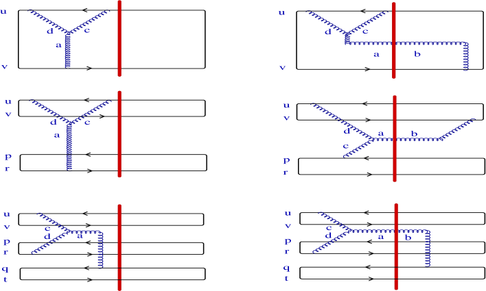
Figure 2: Diagrams corresponding to LLL (plots on the left) and LLR (plots on the right), see the text. The diagrams include one ($\propto 1/N$, top), two ($\propto 1/N^{2}$, middle) and three ($\propto 1/N^{3}$, bottom) active dipoles.

To proceed further we go to the dipole model limit, in which the action of the different terms can be explicitly computed and is illustrated in Figure 2. With $s(x,y)$ the $S$-matrix for a dipole, the kernel (8) can be separated [5] into three pieces containing one, two or three active dipoles with the corresponding $1/N$ suppression factors,

$$\chi^{2)}\Sigma[s]=\left(\chi^{2)}_{1/N}+\chi^{2)}_{1/N^{2}}+\chi^{2)}_{1/N^{3}}\right)\Sigma[s].$$ (9)

$\chi^{2)}_{1/N}$ is found to vanish. Thus the solution to next-to-leading order in the EOMs does not yield leading $1/N$ corrections and, therefore, it does not provide a correction to the BK equation [7]. $\chi^{2)}_{1/N^{2}}$ and $\chi^{2)}_{1/N^{3}}$ cannot be fully recast in terms of dipoles. Noting that any wave function or weight functional of a gluonic/dipole configuration has to be completely symmetric under the exchange of any number of gluons/dipoles, we get

$$\chi^{2)}_{1/N^{2}}\Sigma[s]=-\frac{i}{(2\pi)^{2}}\,\frac{1}{N^{2}}\int d^{2}z\,\Big{\{}[\partial_{i}(R\!-\!P)(U\!\stackrel{{\scriptstyle\leftrightarrow}}{{\partial_{i}}}\!V)$$ (10)

$$-\partial(V\!-\!U)(P\!\stackrel{{\scriptstyle\leftrightarrow}}{{\partial_{i}}}\!R)][N\,\mbox{tr}\{S_{u}^{\dagger}S_{v}S_{z}^{\dagger}S_{r}S_{p}^{\dagger}S_{z}\}]+\partial_{i}(V\!-\!U)$$

$$\times(R\!-\!P)\stackrel{{\scriptstyle\leftrightarrow}}{{\partial_{i}}}(V\!-\!U)\left[\mbox{tr}\{S_{z}^{\dagger}S_{v}S_{p}^{\dagger}S_{r}\}\mbox{tr}\{S_{u}^{\dagger}S_{z}\}-\mbox{tr}\{S_{u}^{\dagger}S_{z}S_{p}^{\dagger}S_{r}\}\mbox{tr}\{S_{z}^{\dagger}S_{v}\}\right.$$

$$\left.+\mbox{tr}\{S_{p}^{\dagger}S_{z}S_{u}^{\dagger}S_{r}\}\mbox{tr}\{S_{z}^{\dagger}S_{v}\}-\mbox{tr}\{S_{p}^{\dagger}S_{v}S_{z}^{\dagger}S_{r}\}\mbox{tr}\{S_{u}^{\dagger}S_{z}\}\right]\Big{\}}\,\frac{\delta^{2}\Sigma[s]}{\delta s(p,r)\delta s(u,v)}\,\,,$$

$$\chi^{2)}_{1/N^{3}}\Sigma[s]=-\frac{i}{2}\,\frac{1}{(2\pi)^{2}}\,\frac{1}{N^{3}}\int d^{2}z\left[\{\partial_{i}(R\!-\!P)\}\{(T\!-\!Q)\stackrel{{\scriptstyle\leftrightarrow}}{{\partial_{i}}}(V\!-\!U)\}\right]$$

$$\times\left[\mbox{tr}\{S^{\dagger}_{u}S_{v}S^{\dagger}_{q}S_{t}S^{\dagger}_{p}S_{r}\}+\mbox{tr}\{S^{\dagger}_{u}S_{t}S^{\dagger}_{q}S_{r}S^{\dagger}_{p}S_{v}\}+\mbox{tr}\{S^{\dagger}_{z}S_{r}S^{\dagger}_{p}S_{z}S^{\dagger}_{u}S_{v}S^{\dagger}_{q}S_{t}\}\right.$$

$$\left.+\mbox{tr}\{S^{\dagger}_{p}S_{r}S^{\dagger}_{z}S_{v}S^{\dagger}_{u}S_{t}S^{\dagger}_{q}S_{z}\}\right]\frac{\delta^{3}\Sigma[s]}{\delta s(q,t)\delta s(p,r)\delta s(u,v)}\,\,.$$ (11)

3 Conclusions

In this contribution we present the ${\cal O}(\alpha_{s}^{2})$ corrections to the JIMWLK evolution equation coming from the ${\cal O}(g^{3}\rho^{2})$ solution to the classical EOMs. The leading $1/N$ piece in the dipole model limit is found to vanish, thus yielding no correction to the BK equation. Subleading corrections do not show a closed dipole form. While the corrections we compute are certainly not the complete set of ${\cal O}(\alpha_{s}^{2})$ corrections to JIMWLK, they are part of the full solution and may turn to be important to fulfill general requirements of the complete theory of high gluon density QCD like dense-dilute duality [8].

References

References

[1]
McLerran L D and Venugopalan R 1994 Phys. Rev.D 49 2233;
D 49 3352;
D 50 2225
[2]
Iancu E and Venugopalan R 2003
Preprint hep-ph/0303204
[3]
Kovner A 2005 Acta Phys. Polon. B 36 3551;
Triantafyllopoulos D N 2005 ibid. 3593
[4]
Kovner A and Lublinsky M 2005 JHEP0503 001
[5]
Albacete J L, Armesto N and Milhano J G 2006 JHEP0611 074
[6]
Kovchegov Y V 1996 Phys. Rev.D 54 5463;
1997 Phys. Rev.D 55 5445
[7]
Balitsky I 1996 Nucl. Phys.B 463 99;
Kovchegov Y V 1999 Phys. Rev.D 60 034008
[8]
Kovner A and Lublinsky M 2005 Phys. Rev. Lett.94 181603