The role of the gluonic $gg\leftrightarrow ggg$ interactions in early thermalization in ultrarelativistic heavy-ion collisions

Abstract

We “quantify” the role of elastic as well as inelastic $gg\leftrightarrow ggg$ pQCD processes in kinetic equilibration within a pQCD inspired parton cascade. The contributions of different processes to kinetic equilibration are manifested by the transport collision rates. We find that in a central Au+Au collision at RHIC energy pQCD Bremstrahlung processes are much more efficient for momentum isotropization compared to elastic scatterings. For the parameters chosen the ratio of their transport collision rates amounts to $5:1$.

1 Introduction

It was speculated that a strongly coupled quark-gluon plasma (sQGP) Guyl is formed in Au+Au collisions at RHIC. This strong coupling, or strong interaction, makes the QGP to a fluid with very small viscosity. However, how strong the coupling must be in order to generate a quasi-ideal fluid is an open question.

Recently we have developed an on-shell parton cascade including elastic as well as inelastic $gg\leftrightarrow ggg$ pQCD processes to study the issue of thermalization Xu1 . Although the total cross section of the pQCD scatterings is a few $mb$, it is enough to drive the system into thermal equilibrium and also to generate a large elliptic flow $v_{2}$ in noncentral Au+Au collisions Xu2 .

Since with elastic pQCD scatterings alone no thermalization is expected to be achieved Xu1 ; serreau , the inelastic $gg\leftrightarrow ggg$ processes seem to play a leading role in early thermalization, although for the parameters chosen in Xu1 the cross section of $gg\to ggg$ collisions is a factor of 2 smaller than that of elastic scatterings. In order to understand this a transport cross section,

$$\sigma^{tr.}=\int d\theta\frac{d\sigma}{d\theta}sin^{2}\theta\,,$$ (1)

was introduced as a pertinent quantity measuring the contributions of different collision processes to kinetic equilibration dg , since large-angle collisions should contribute more to momentum isotropization. The results (see Fig. 48 in Xu1 ) showed that even due to the almost isotropic distribution of the collision angles in inelastic collisions its transport cross section is only the same as that of elastic scatterings. Therefore one cannot understand why the inclusion of the inelastic processes brings so much to kinetic equilibration. At first sight it seems to be an unsolvable problem. On the other hand, however, there is no reason to believe that momentum isotropization should relate to the angular distribution by means of the transport cross section and not by another formula. The concept of the transport cross section may be more intuitively than mathematically correct. In this work we will find a mathematically correct way to quantify the contribution of different processes to thermal equilibration and compare them with each other. The core issue is the transport collision rate. With this quantity we “quantify” the role of different collision processes in kinetic equilibration.

2 Parton cascade

The buildup of the parton cascade is based on the stochastic interpretation of the transition rate. This guarantees detailed balance, which is, by contrast, difficult when using the geometrical concept of the cross section molnar , especially for multiple scatterings like $ggg\to gg$. The particular feature of the numerical implementation in the parton cascade is the subdivision of space into small cell units. In cells the transition probabilities are evaluated for random sampling whether a particular scattering occurs or not. The smaller the cells, the more locally transitions will be realized.

The three-body gluonic interactions are described by the matrix element gb

$$|{\cal M}_{gg\to ggg}|^{2} = \frac{9g^{4}}{2}\frac{s^{2}}{({\bf q}_{\perp}^{2}+m_{D}^{2})^{2}}\,\frac{12g^{2}{\bf q}_{\perp}^{2}}{{\bf k}_{\perp}^{2}[({\bf k}_{\perp}-{\bf q}_{\perp})^{2}+m_{D}^{2}]}\times$$ (2)

$$\times\,\Theta(k_{\perp}\Lambda_{g}-\cosh y)\,.$$

The suppression of the radiation of soft gluons due to the Landau-Pomeranchuk-Migdal (LPM) effect biro ; wong ; Xu1 , which is expressed via the step function in Eq. (2), is modeled by the consideration that the time of the emission, $\sim\frac{1}{k_{\perp}}\cosh y$, should be smaller than the time interval between two scatterings or equivalently the gluon mean free path $\Lambda_{g}$. This leads to a lower cutoff for $k_{\perp}$ and to a decrease of the total cross section.

In this work we simulate the time evolution of gluons produced in a central Au+Au collision at RHIC energy. The initial gluons are taken as minijets with transverse momentum being greater than $1.4$ GeV, which are produced via semi-hard nucleon-nucleon collisions. Using the Glauber geometry the gluon number is initially about $700$ per momentum rapidity. These gluons take about $60\%$ of the total energy entered in the collision. Choosing such an initial condition and performing a simulation including Bremsstrahlung processes we obtain $dE_{T}/dy$ about $640$ GeV at midrapidity at a final time of $5$ fm/c, at which the energy density of gluons decreases to the critical value of $1$ GeV/$\mbox{fm}^{3}$. The value of $dE_{T}/dy$ obtained from the simulation is comparable with that from the experimental measurements at RHIC.

We concentrate on the central region: $0<x_{T}<1.5$ fm and $-0.2<\eta<0.2$, where $\eta$ denotes the space-time rapidity. Results which will be shown below are obtained in this region by ensemble average.

The importance of including inelastic pQCD $gg\leftrightarrow ggg$ processes to momentum isotropization is clearly demonstrated in Fig. 1, where the time evolution of the averaged momentum anisotropy, $<p_{Z}^{2}/E^{2}>$, is depicted.

Figure 1: Momentum anisotropy.

$p_{Z}$ and $E$ are, respectively, longitudinal momentum and energy of a gluon. The average is computed over all gluons in the central region. As comparison we have also performed a simulation with pure elastic processes starting with the same initial conditions. From Fig. 1 we see that while the gluon system is still far from kinetic equilibrium in the simulation with pure elastic scatterings (dashed curve), the momentum anisotropy relaxes to the value at equilibrium, $1/3$, in the simulation including inelastic processes (solid curve).

We fit the time evolution of the momentum anisotropy using the standard relaxation formula

$$F(t)=\frac{1}{3}+\left(\left<\frac{p_{Z}^{2}}{E^{2}}\right>(t_{0})-\frac{1}{3}\right)\exp\,(-\frac{t-t_{0}}{\theta(t_{0})})\,.$$ (3)

For simplicity we label now the momentum anisotropy by $Q:=<p_{Z}^{2}/E^{2}>$. $F(t)$ is only equal to $Q(t)$ at $t=t_{0}$. For fixed $t_{0}$ the relaxation time $\theta$ is a constant with respect to $t$. Such a fit can be done at every time point $t_{0}$. The two thin dotted curves in Fig. 1 are fits with $\theta=0.9$ fm/c at $t_{0}=0.3$ fm/c and $\theta=2.4$ fm/c at $t_{0}=1.2$ fm/c. We find that an isotropic state is achieved at about $1.0$ fm/c in the simulation including inelastic scattering processes. Moreover, we see that the relaxation time $\theta$ is generally time dependent. The two values of $\theta$ in the fits are obtained by guessing. Actually $\theta$ can be calculated exactly, since in order to make a local fit one should request that the time derivative of $F(t)$ and $Q(t)$ are equal at $t=t_{0}$. This leads to

$$\left.\dot{Q}(t)\right|_{t=t_{0}}=\left.\dot{F}(t)\right|_{t=t_{0}}=-(Q(t_{0})-Q_{eq.})\,\frac{1}{\theta(t_{0})}\,,$$ (4)

with $Q_{eq.}=1/3$. Changing $t_{0}$ to $t$ gives

$$\frac{\dot{Q}(t)}{Q_{eq.}-Q(t)}=\frac{1}{\theta(t)}.$$ (5)

Equation (5) expresses the relaxation rate $1/\theta$ of the momentum anisotropy. In the next section we analytically separate the relaxation rate into different terms corresponding particle diffusion and various scattering processes, and we define the transport collision rate which quantifies the contribution of a certain process to momentum isotropization.

3 Transport collision rate

For evaluating the momentum anisotropy at a certain space point one has to go to its co-moving frame, in which we have

$$Q(t)=\left.\left<\frac{p_{Z}^{2}}{E^{2}}\right>\right|_{x=0}=\frac{1}{n}\int\frac{d^{3}p}{(2\pi)^{3}}\frac{p_{Z}^{2}}{E^{2}}\,f(p,x=0,t)\,.$$ (6)

Taking the derivative in time gives

$$\dot{Q}(t)=\frac{1}{n}\int\frac{d^{3}p}{(2\pi)^{3}}\frac{p_{Z}^{2}}{E^{2}}\,\frac{\partial f}{\partial t}-Q(t)\frac{1}{n}\int\frac{d^{3}p}{(2\pi)^{3}}\frac{\partial f}{\partial t}\,.$$ (7)

We replace $\partial f/\partial t$ by

$$\frac{\partial f}{\partial t}=-\frac{\vec{p}}{E}\vec{\nabla}f+C_{22}+C_{23}+C_{32}$$ (8)

according to the Boltzmann equation. $C_{22}$, $C_{23}$ and $C_{32}$ denote, respectively, the collision term of $gg\to gg$, $gg\to ggg$ and $ggg\to gg$ process. It is obvious that the contribution of different processes to $\dot{Q}$ is additive. Except for a static system the diffusion term in Eq. (8) generally has contribution to $\dot{Q}(t)$, which we denote by $W_{diff.}$. $C_{22}$ has no contribution to the second integral in Eq. (7) due to particle number conservation. The same is also for the sum of $C_{23}$ and $C_{32}$ at chemical equilibrium. We rewrite Eq. (7) to

$$\dot{Q}(t)=W_{diff.}(t)+W_{22}(t)+W_{23}(t)+W_{32}(t)\,,$$ (9)

where $W_{22}$, $W_{23}$ and $W_{32}$ correspond to the $gg\to gg$, $gg\to ggg$ and $ggg\to gg$ process, respectively. According to (5) we then obtain

$$\frac{1}{\theta(t)}=R^{tr.}_{diff}(t)+R^{tr.}_{22}(t)+R^{tr.}_{23}(t)+R^{tr.}_{32}(t)\,,$$ (10)

where we define

$$R^{tr.}_{i}(t):=\frac{W_{i}(t)}{Q_{eq.}-Q(t)}\,.$$ (11)

We see that the relaxation rate of kinetic equilibration, $1/\theta$, is separated into additive parts corresponding to particle diffusion and collision processes. $R^{tr.}_{22}$, $R^{tr.}_{23}$ and $R^{tr.}_{32}$ stand for the transport collision rates of the respective interactions and quantify their contributions to kinetic equilibration. The extension to more than three-body processes is straightforward because the collision term is additive. We note that the definition of $R^{tr.}_{i}$ in Eq. (11) depends on which momentum anisotropy we are looking at. If one defines $<|p_{Z}|/E>$ as the momentum anisotropy for instance, the form $R^{tr.}_{i}$ will change accordingly.

Putting the explicit expression of the collision term via the matrix element of transition into (8), we obtain explicit expressions for $W_{i}$, which are summarized in the following:

$$W_{22}(t)= n<v_{rel}\,\tilde{\sigma}_{22}>_{2}-n\left<v_{rel}\frac{p^{2}_{1Z}}{E^{2}_{1}}\,\sigma_{22}\right>_{2}\,,$$ (12)

$$W_{23}(t)= \frac{3}{2}\,n<v_{rel}\,\tilde{\sigma}_{23}>_{2}-n\left<v_{rel}\frac{p^{2}_{1Z}}{E^{2}_{1}}\,\sigma_{23}\right>_{2}$$ (13)

$$-\frac{1}{2}\,Q(t)\,n<v_{rel}\,\sigma_{23}>_{2}\,,$$

$$W_{32}(t)= \frac{1}{3}n^{2}\left<\frac{\tilde{I}_{32}}{8E_{1}E_{2}E_{3}}\right>_{3}-\frac{1}{2}n^{2}\left<\frac{p^{2}_{1Z}}{E^{2}_{1}}\frac{I_{32}}{8E_{1}E_{2}E_{3}}\right>_{3}$$ (14)

$$+\frac{1}{6}\,Q(t)\,n^{2}\left<\frac{I_{32}}{8E_{1}E_{2}E_{3}}\right>_{3}\,,$$

where

$$\tilde{\sigma}_{22}:= \frac{1}{2s}\frac{1}{2!}\int d\Gamma^{{}^{\prime}}_{1}d\Gamma^{{}^{\prime}}_{2}\,\frac{p^{{}^{\prime}2}_{1Z}}{E^{{}^{\prime}2}_{1}}\,|{\cal M}_{12\to 1^{{}^{\prime}}2^{{}^{\prime}}}|^{2}\times$$ (15)

$$\times\,(2\pi)^{4}\delta^{(4)}(p_{1}+p_{2}-p^{{}^{\prime}}_{1}-p^{{}^{\prime}}_{2})$$

$$\tilde{\sigma}_{23}:= \frac{1}{2s}\frac{1}{3!}\int d\Gamma^{{}^{\prime}}_{1}d\Gamma^{{}^{\prime}}_{2}d\Gamma^{{}^{\prime}}_{3}\,\frac{p^{{}^{\prime}2}_{1Z}}{E^{{}^{\prime}2}_{1}}\,|{\cal M}_{12\to 1^{{}^{\prime}}2^{{}^{\prime}}3^{{}^{\prime}}}|^{2}\times$$ (16)

$$\times\,(2\pi)^{4}\delta^{(4)}(p_{1}+p_{2}-p^{{}^{\prime}}_{1}-p^{{}^{\prime}}_{2}-p^{{}^{\prime}}_{3})$$

$$I_{32}:= \frac{1}{2!}\int d\Gamma^{{}^{\prime}}_{1}d\Gamma^{{}^{\prime}}_{2}\,|{\cal M}_{123\to 1^{{}^{\prime}}2^{{}^{\prime}}}|^{2}\times$$ (17)

$$\times\,(2\pi)^{4}\delta^{(4)}(p_{1}+p_{2}+p_{3}-p^{{}^{\prime}}_{1}-p^{{}^{\prime}}_{2})$$

$$\tilde{I}_{32}:= \frac{1}{2!}\int d\Gamma^{{}^{\prime}}_{1}d\Gamma^{{}^{\prime}}_{2}\,\frac{p^{{}^{\prime}2}_{1Z}}{E^{{}^{\prime}2}_{1}}\,|{\cal M}_{123\to 1^{{}^{\prime}}2^{{}^{\prime}}}|^{2}\times$$ (18)

$$\times\,(2\pi)^{4}\delta^{(4)}(p_{1}+p_{2}+p_{3}-p^{{}^{\prime}}_{1}-p^{{}^{\prime}}_{2})$$

with $d\Gamma_{i}=d^{3}p_{i}/(2\pi)^{3}2E_{i}$ for short. $\sigma_{22}$ and $\sigma_{23}$ denote the standard pQCD cross section of the $gg\to gg$ and $gg\to ggg$ process, respectively. $v_{rel}=s/2E_{1}E_{2}$ is the relative velocity. $<>_{2}$ and $<>_{3}$ symbolize, respectively, an ensemble average over pairs and triplets of incoming particles. In the parton cascade simulations $f(p,x,t)\approx\sum_{i}\delta^{(3)}(p-p_{i})\delta^{(3)}(x-x_{i}(t))$, and we can approximately evaluate the averages $<>_{2}$ and $<>_{3}$ in local cells which have small volume, but a sufficient number of (test) particles to achieve high statistics.

The expression of $W_{i}$s in (12), (13) and (14) indicates the difference of the gain and loss in the momentum isotropization within one collision. The influence of the distribution of the collision angle on momentum isotropization is implicitly contained. However, the expression of the transport collision rate $R^{tr.}_{i}$ is clearly different from $n<v_{rel}\sigma^{tr.}_{i}>_{2}$ by the formula (1). (The index $i$ denotes $22$ or $23$.) Only in the special case that all particles are moving along the $Z-$axis (irrespective of $\pm$ sign) and have the same energy $E$,

$$f(p,x,t)\propto\delta(p_{X})\delta(p_{Y})\delta(p_{Z}-E)+\delta(p_{X})\delta(p_{Y})\delta(p_{Z}+E)\,,$$ (19)

the lab frame is the CM system for every colliding pair. In this case $p^{{}^{\prime}2}_{1Z}/E^{{}^{\prime}2}_{1}=\cos^{2}\theta^{*}$ and

$$R^{tr.}_{i}\sim n<v_{rel}\sigma^{tr.}_{i}>_{2}\,.$$ (20)

This result does not depend on the chosen direction of initial momentum. The only necessary conditions are that all particles move along the same direction and have the same energy. If we define the momentum anisotropy as $<|p_{Z}|/E>$, $R^{tr.}_{i}$ maintains its form (20), but $\sigma^{tr.}_{i}$ is changed to

$$\sigma^{tr.}_{i}=\int d\theta^{*}\frac{d\sigma_{i}}{d\theta^{*}}(1-\cos\theta^{*})\,.$$ (21)

Figure 2 shows the transport rates $R^{tr.}_{i}$ obtained from simulations employing the parton cascade.

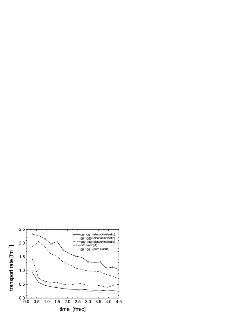
Figure 2: Transport rate.

The solid, dashed and dash-dotted curves depict, respectively, the transport collision rates $R^{tr.}_{22}$, $R^{tr.}_{23}$ and $R^{tr.}_{32}$ calculated in the simulation with both elastic and inelastic collisions. We realize the dominance of inelastic collisions in kinetic equilibration by computing the ratio $(R^{tr.}_{23}+R^{tr.}_{32})/R^{tr.}_{22}\approx 5$. The thin dotted curve in Fig. 2 presents $R^{tr.}_{22}$ in the simulation with pure elastic processes. When comparing this with the solid curve one cannot realize much difference.

The contribution of particle diffusion to kinetic equilibration, $R^{tr.}_{diff.}$, calculated in the simulation with both elastic and inelastic processes, is depicted in Fig. 2 by the symbols multiplied by $-1$. $R^{tr.}_{diff.}$, which is expressed by

$$R^{tr.}_{diff.}(t)=\frac{1}{Q_{eq.}-Q(t)}\frac{1}{n}\int\frac{d^{3}p}{(2\pi)^{3}}\frac{\vec{p}}{E}\,\cdot\vec{\nabla}f\,\left(Q(t)-\frac{p_{Z}^{2}}{E^{2}}\right)\,,$$ (22)

is not computed at a certain time as performed for the transport collision rates, because of the inaccurate extraction of $\vec{\nabla}f$. The diffusion rate is obtained by explicit counting of the particles which come in as well as go out of the central region within a time interval. Although the extraction of $R^{tr.}_{diff.}$ has a much larger statistical fluctuation, the sum $R^{tr.}_{diff.}+R^{tr.}_{22}+R^{tr.}_{23}+R^{tr.}_{32}$ gives a value consistent with the relaxation rate $1/\theta(t)$ as one would calculate via $\dot{Q}(t)/(Q_{eq.}-Q(t))$ directly from Fig. 1.

We also see that $R^{tr.}_{diff.}$ has a negative contribution to momentum isotropization and is quite large. We did not plot $-R^{tr.}_{diff.}$ from the simulation with pure elastic processes. It is slightly smaller than $R^{tr.}_{22}$ (thin dotted curve). We see that there is a big difference in the diffusion rate in both simulations. To understand this we assume Bjorken’s space-time picture of central ultrarelativistic heavy-ion collisions bjork and use the relation derived by Baym baym :

$$\frac{\vec{p}}{E}\cdot\vec{\nabla}f\approx\frac{p_{Z}}{E}\frac{\partial f}{\partial Z}=-\frac{p_{Z}}{t}\frac{\partial f}{\partial p_{Z}}\,.$$ (23)

Inserting Eq. (23) into Eq. (22) and calculating partial integrals give

$$R^{tr.}_{diff.}(t)\approx\frac{-2}{(Q_{eq.}-Q(t))\,t}\,\left(Q(t)-\left<\frac{p_{Z}^{4}}{E^{4}}\right>(t)\right)\,.$$ (24)

The formula confirms that $R^{tr.}_{diff.}$ is always negative. Using the approximation $<p_{Z}^{4}/E^{4}>\approx Q^{2}$ one can also realize that the larger is Q, the larger $-R^{tr.}_{diff.}$ is.

We have seen that only in an extreme case the transport collision rate can be reduced to a formula directly proportional to the transport cross section: $R^{tr.}\sim n<v_{rel}\,\sigma^{tr.}>_{2}$. It is interesting to know how the calculated transport collision rates differ from $n<v_{rel}\,\sigma^{tr.}>_{2}$. Such a comparison is necessary for understanding why the concept of transport cross section cannot explain the strong effect when including inelastic scattering processes. In Fig. 3 we depict $n<v_{rel}\,\sigma^{tr.}>_{2}$ calculated from the cascade simulations.

Figure 3: “Transport collision rate” in the concept of transport cross section.

At first we look at the results in the simulation with both elastic and inelastic collisions and calculate the inelastic to elastic ratio (dashed versus solid curve). It is almost a constant around $1.7$ in time, which indicates the dominance of the $gg\to ggg$ scattering processes in kinetic equilibration. Comparing Fig. 3 to Fig. 2 we realize that the results concerning elastic scatterings have no strong difference. On the contrary, $R^{tr.}_{23}$ is a factor of $2.5$ larger than $n<v_{rel}\,\sigma^{tr.}_{23}>_{2}$. The pQCD $gg\to ggg$ process is much more efficient for kinetic equilibration than one would expect via the transport cross section.

4 Bremsstrahlung process and the LPM effect

It is intuitively clear that a $2\to 3$ process will bring one more particle towards isotropy than a $2\to 2$ process. The kinematic factor should be $3/2$ and appears in Eq. (13) when assuming the decompositions

$$\left<v_{rel}\frac{p^{2}_{1Z}}{E^{2}_{1}}\,\sigma\right>_{2}\,\approx Q(t)<v_{rel}\,\sigma>_{2}\,.$$ (25)

Analogously we compare $W_{23}$ to $W_{32}$. The sum of the last term in Eq. (13) and Eq. (14) comes from the second term in Eq. (7) with $C_{23}+C_{32}$ instead of $\partial f/\partial t$ and should be zero at chemical equilibrium: we obtain

$$n<v_{rel}\,\sigma_{23}>_{2}=\frac{1}{3}n^{2}\left<\frac{I_{32}}{8E_{1}E_{2}E_{3}}\right>_{3}\,,$$ (26)

or equivalently $R_{23}=\frac{2}{3}R_{32}$. Assuming further the decomposition

$$\left<\frac{p^{2}_{1Z}}{E^{2}_{1}}\frac{I_{32}}{8E_{1}E_{2}E_{3}}\right>_{3}\,\approx Q(t)\left<\frac{I_{32}}{8E_{1}E_{2}E_{3}}\right>_{3}\,,$$ (27)

we have

$$W_{23}(t) \approx \frac{3}{2}(n<v_{rel}\,\tilde{\sigma}_{23}>_{2}-Q(t)\,n<v_{rel}\,\sigma_{23}>_{2})\,,$$

$$W_{32}(t) \approx \frac{1}{3}n^{2}\left<\frac{\tilde{I}_{32}}{8E_{1}E_{2}E_{3}}\right>_{3}-Q(t)\frac{1}{3}n^{2}\left<\frac{I_{32}}{8E_{1}E_{2}E_{3}}\right>_{3}.$$

These approximate expansions together with Eq. (26) lead to $W_{23}\approx\frac{3}{2}W_{32}$ and $R^{tr.}_{23}\approx\frac{3}{2}R^{tr.}_{32}$ at chemical equilibrium. Alone due to the kinematic reason a $2\to 3$ process is $50\%$ more efficient in kinetic equilibration than a $2\to 2$ or a $3\to 2$ process, when $\sigma_{22}=\sigma_{23}$ and $\tilde{\sigma}_{22}=\tilde{\sigma}_{23}$.

The LPM effect stems from the interference of the radiated gluons (originally photons in the QED medium) by multiple scattering of a parton though a medium. This is a coherent effect which leads to suppression of radiation of gluons with certain modes $(w,\vec{k})$. $w$ and $\vec{k}$ denote energy and momentum of a gluon respectively. Heuristically there is no suppression for gluons with a formation time $\tau=w/k_{T}^{2}$ smaller than the mean free path. This is called the Bethe-Heitler limit, where the gluon radiations induced at a different space-time point in the course of the propagation of a parton can be considered as independent events. These events within the Bethe-Heitler regime have been included in the parton cascade calculations. Radiation of other gluon modes with coherent suppression completely dropped out, which is indicated by the $\Theta$-function in the matrix element (2). The inclusion of those radiations would speed up thermalization. How to implement the coherent effect into a transport model solving the Boltzmann equation is a challenge.

The $\Theta$-function in the matrix element (2) results in a cut-off for $k_{T}$, the transverse momentum of a radiated gluon, $k_{T}>1/\Lambda_{g}$, where $\Lambda_{g}$ is the mean free path of a gluon. A higher value of the cut-off will decrease the total cross section of a $gg\to ggg$ collision on the one hand and make the collision angles large on the other hand. The latter leads to a large efficiency for momentum isotropization. Varying the cut-off downwards to a smaller value one would enter into the LPM suppressed regime. Although parton cascade calculations set up with smaller cut-offs cannot completely take the LPM effect into account, one can roughly estimate the contribution of the coherent effect to kinetic equilibration. Such calculations will be done in a subsequent paper.

5 Conclusion

Employing the parton cascade we have investigated the importance of including pQCD Bremsstrahlung processes to thermalization. The question addressed is how to understand the observed fast equilibration in theoretical terms. The special emphasis is put on expressing the transport collision rate in a correct manner. The concept of transport cross section only gives a qualitative understanding of the dominant contribution of large-angle scatterings to momentum isotropization but not a correct way to manifest the various contributions. In case we are studying parton thermalization in a central Au+Au collision at RHIC energy the old concept of the transport cross sections would strongly underestimate the contribution of $gg\to ggg$ to kinetic equilibration. The correct results showed that the inclusion of pQCD Bremsstrahlung processes increases the efficiency by a factor of $5$ for thermalization. The large efficiency stems partly from the increase of particle number in the final state of $gg\to ggg$ collisions, but mainly from the almost isotropic angular distribution in Bremsstrahlung processes due to the effective implementation of LPM suppression. The detailed understanding of the latter has to be developed in future investigations.

References

- (1) Miklos Gyulassy and Larry McLerran, Nucl.Phys.A 750, (2005) 30-63.
- (2) Zhe Xu and Carsten Greiner, Phys.Rev.C 71, (2005) 064901.
- (3) Zhe Xu and Carsten Greiner, Proceedings of Quark Matter 2006, hep-ph/0509324.
- (4) J. Serreau and D. Schiff, J. High Energy Phys. 0111, (2001) 039.
- (5) P. Danielewicz and M. Gyulassy, Phys.Rev.D 31, (1985) 53.
- (6) D. Molnar, Proceedings of Quark Matter 1999, Nucl.Phys.A 661, (1999) 205-260.
- (7) J.F. Gunion and G. Bertsch, Phys.Rev.D 25, (1982) 746.
- (8) T.S. Biro et al, Phys.Rev.C 48, (1993) 1275.
- (9) S.M.H. Wong, Nucl.Phys.A 607, (1996) 442.
- (10) J.D. Bjorken, Phys.Rev.D 27, (1983) 140.
- (11) G. Baym, Phys.Lett.B 138, (1984) 18.