Novel Effects in Electroweak Breaking from a Hidden Sector

Abstract

The Higgs boson offers a unique window to hidden sector fields $S_{i}$, singlets under the Standard Model gauge group, via the renormalizable interactions $|H|^{2}S_{i}^{2}$. We prove that such interactions can provide new patterns for electroweak breaking, including radiative breaking by dimensional transmutation consistent with LEP bounds, and trigger the strong enough first order phase transition required by electroweak baryogenesis.

1. Introduction. The Standard Model (SM) of electroweak and strong interactions can not be considered as a fundamental theory, since it fails to provide an answer to many open questions (the hierarchy, cosmological constant and flavor problems, the origin of baryons, the Dark Matter and Dark Energy of the Universe, …), but rather as an effective theory with a physical cutoff $\Lambda$ that most likely shall be probed at the LHC experiment. Many SM extensions, e.g. string theory, contain hidden sectors with a matter content transforming non-trivially under a hidden sector gauge group but singlet under the SM gauge group. It has recently been noticed that the SM Higgs field $H$ plays a very special role with respect to such hidden sector since it can provide a window (a portal hidden0 ) into it through the renormalizable interaction $|H|^{2}S_{i}^{2}$ where the bosons $S_{i}$ are SM singlets.

This coupling to the hidden sector can have important implications both theoretically and for LHC phenomenology as has been discussed in recent literature hidden0 ; hidden1 ; hidden2 ; hidden3 ; hidden4 ; hidden5 ; hidden6 ; hiding . In this letter we show that the presence of a hidden sector may have dramatic consequences for electroweak symmetry breaking (in particular it enables new patterns of electroweak symmetry breaking, including radiative breaking by dimensional transmutation consistent with present LEP bounds on the Higgs mass) and for electroweak baryogenesis (it makes easy to get a first order phase transition as strong as required for electroweak baryogenesis). Furthermore, under mild assumptions those hidden sector fields are stable and can constitute the Dark Matter of the Universe.

2. Electroweak breaking. We will consider a set of $N$ fields $S_{i}$ coupled to the SM Higgs doublet by the (tree-level) potential

$$V_{0}=\,m^{2}H^{\dagger}H+\lambda\,(H^{\dagger}H)^{2}+\zeta^{2}H^{\dagger}H\sum_{i}S_{i}^{2}.$$ (1)

We will assume for the moment that the fields $S_{i}$ are massless so they only will get a mass from electroweak breaking. In the background Higgs field configuration defined by $\langle H^{0}\rangle=h/\sqrt{2}$, the one-loop effective potential (in Landau gauge and $\overline{MS}$ scheme) is given by

$$V=\frac{m^{2}}{2}h^{2}+\frac{\lambda}{4}h^{4}+\sum_{\alpha}\frac{N_{\alpha}M_{\alpha}^{4}}{64\pi^{2}}\left[\ln\frac{M_{\alpha}^{2}}{Q^{2}}-C_{\alpha}\right]\ ,$$ (2)

where $\alpha=\{S,Z,W,t,h,G\}$ for singlet hidden sector fields, gauge bosons, top, Higgs and Goldstones respectively, with $N_{\alpha}=\{N,3,6,-12,1,3\}$. Inspired by the case of stops, we choose $N=12$ for our numerical work. Next, $C_{\alpha}=3/2$ for fermions or scalars and $5/6$ for gauge bosons, and the $h$-dependent masses are $M_{S}^{2}=\zeta^{2}h^{2}$, $M_{Z}^{2}=(g^{2}+g^{\prime 2})h^{2}/4$, $M_{W}^{2}=g^{2}h^{2}/4$, $M_{t}^{2}=h_{t}^{2}h^{2}/2$, $M_{h}^{2}=3\lambda h^{2}+m^{2}$, $M_{G}^{2}=\lambda h^{2}+m^{2}$. The renormalization scale $Q$ enters explicitly in the one-loop logarithmic correction and implicitly through the dependence of all couplings and fields on $t=\ln Q$ in such a way that $dV/dt=0$ is satisfied. For now we simply choose the scale as $Q=M_{t}(v)$ and fix the parameters (at that scale) to get $\langle h\rangle=v\simeq 246$ GeV.

For $\zeta^{2}<h_{t}^{2}/2\simeq 0.65$ the one-loop term in (2) is dominated by the standard top contribution but for $\zeta^{2}>h_{t}^{2}/2$ hidden scalars start to dominate. The structure of the effective potential is best described by using Fig. 1. Consider first the $(\zeta,\lambda)$-plane in the upper plot. Besides the lines of constant $M_{h}$, we can distinguish four regions. i) The region below the blue line [defined by $V^{\prime\prime}(v)=0$] is forbidden: there $M_{h}^{2}<0$. The extremal at $h=v$ is a maximum that degenerates into an inflection point on the blue line. ii) In the region above the blue line but below the red line there is an electroweak minimum, but it is a false minimum with respect to the (true) minimum at the origin. The red line is defined by $V(v)=V(0)$, i.e. both minima, at the origin and at $h=v$, are degenerate on that line. This region ii) is therefore unphysical without a mechanism to populate the metastable minimum (in general, the true minimum at the origin would be preferred at high temperature and the electroweak transition would never take place). iii) In the region above the red line but below the green line [defined by $V^{\prime\prime}(0)=0$] the electroweak minimum is stable and there is a barrier separating the false minimum at the origin from the electroweak minimum ($m^{2}>0$). This region is very interesting for two reasons:

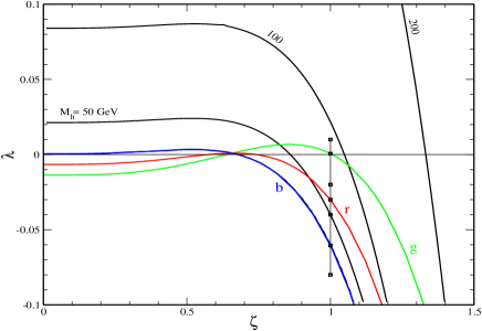
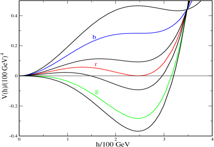
Figure 1: Upper plot: In the plane $(\zeta,\lambda)$, the green line corresponds to the condition $V^{\prime\prime}(0)=0$, the red to $V(v)=V(0)$ and the blue to $V^{\prime\prime}(v)=0$. Black solid lines correspond to the indicated values of $M_{h}$. Lower plot: Potential for $\zeta=1.0$ and different values of $\lambda$ (or $M_{h}$) as marked on the vertical line in upper plot.

• The barrier between both minima (at zero temperature) will produce an overcooling of the Higgs field at the origin at finite temperature, strengthening the first order phase transition (see below).

• Electroweak symmetry breaking is not associated with the presence of a tachyonic mass at the origin, as in the SM. Instead it is triggered by radiative corrections via the mechanism of dimensional transmutation.

The minimum at the origin becomes a maximum at the green line. In fact the green line corresponds to the conformal case where $m^{2}=0$ and electroweak breaking proceeds by pure dimensional transmutation (see also Nicolai ). iv) Finally, in the region above the green line the origin is a maximum as in the SM, with $m^{2}<0$.

Notice that, while $\lambda>0$ is required in the SM case ($\zeta=0$ axis), now $\lambda<0$ is accessible for sufficiently large $\zeta$. The shape of the potential for the different cases is illustrated by the lower plot of Fig. 1, where $\zeta=1$ has been fixed and we vary $\lambda$ as indicated by the vertical line in the upper plot of Fig. 1. From bottom-up the potentials have decreasing values of $\lambda$. The lowest potential corresponds to $\lambda=0.01$ and has the conventional maximum at the origin. The green potential corresponds to the conformal case where $m^{2}=0$ (in this particular example also $\lambda$ is zero!). The next line corresponds to $\lambda=-0.02$ with a barrier between the origin and the electroweak minimum while for the red potential the two minima become degenerate. The next line corresponds to the potential for $\lambda=-0.04$ where the electroweak minimum is already a false minimum, which becomes an inflection point at the blue line where $M_{h}=0$. Finally the highest line corresponds to $\lambda=-0.08$ and the electroweak extremal is a maximum (the potential has a minimum somewhere else, for some $\langle h\rangle>v$. If $\zeta^{2}$ were smaller, $\zeta^{2}\stackrel{{\scriptstyle<}}{{{}_{\sim}}}h_{t}^{2}/2$, the potential would instead be destabilized due to $\lambda<0$.).

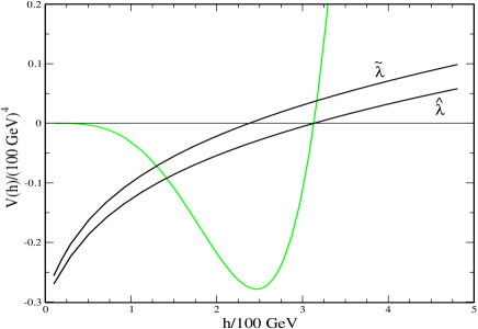
Figure 2: Green: Effective potential for the conformal case. Black: running $\tilde{\lambda}$ and $\hat{\lambda}$, with $Q=M_{t}(h)$.

In order to have a better understanding of the phenomenon of radiative electroweak breaking by dimensional transmutation in this setting consider the conformal case with $m^{2}=0$. Then improve the one-loop effective potential of Eq. (2) by including the running with the renormalization scale of couplings and wave functions. We use for that the SM renormalization group equations (RGEs) supplemented by the effects of $S_{i}$ loops plus the RGEs for the new couplings to the hidden sector (see eqPRD for details). The RGE-improved effective potential is scale independent and we can take advantage of that to take $Q=M_{t}(h)$ as a convenient choice to evaluate the potential at the field value $h$ (with all couplings ran to that particular renormalization scale). This results in a “tree-level” approximation $V\simeq(1/4)\hat{\lambda}h^{4}$ with lambdaeff

$$\hat{\lambda}\equiv\lambda+\sum_{\alpha}\frac{N_{\alpha}\kappa_{\alpha}^{2}}{64\pi^{2}}\left[\ln\frac{\kappa_{\alpha}}{h_{t}^{2}}-C_{\alpha}\right]\ ,$$ (3)

where the $\kappa_{\alpha}$’s are coupling constants, defined by the masses as $M_{\alpha}^{2}=(1/2)\kappa_{\alpha}h^{2}$. The behavior of the one-loop potential as a function of $h$ is captured by the “tree-level” approximation above through the running of $\hat{\lambda}$ with the renormalization scale, linked to a running with $h$ by the choice $Q=M_{t}(h)$. To illustrate this, we show in Fig. 2 the effective potential for this conformal case (green lines in Fig. 1) with $m^{2}=0$ and $\zeta=1$, together with the effective quartic coupling $\hat{\lambda}(h)$. We can see that the scale of dimensional transmutation is related to the scale at which the potential crosses through zero. The structure of the potential is then determined by the evolution of $\hat{\lambda}$: for small $h$, $\hat{\lambda}<0$ destabilizes the origin while, for larger $h$, $\hat{\lambda}>0$ stabilizes the potential curving it upwards in the usual way.

We can define a different effective coupling, $\tilde{\lambda}$, by the approximation $\partial V/\partial h\simeq\tilde{\lambda}h^{3}$, which fixes $\tilde{\lambda}$ to be given by (3) with $C_{\alpha}\rightarrow C_{\alpha}-1/2$. Fig. 2 shows that $\tilde{\lambda}$ crosses through zero precisely at the minimum of the potential. This shows then how the electroweak scale is generated by dimensional transmutation: a suitably defined effective quartic Higgs coupling turns from positive to negative values, with $v$ given by the implicit condition $\tilde{\lambda}(v)=0$. Needless to say, such running of $\tilde{\lambda}$ would not be possible in the SM and is due to the effect of $\zeta$ in the RGEs, which counterbalances the effect of $h_{t}$.

3. Electroweak phase transition. In the presence of hidden sector fields $S_{i}$ coupled to the SM Higgs as in Eq. (1) the electroweak phase transition is strengthened by: a) The thermal contribution from $S_{i}$, if $\zeta$ is large enough. This fact was known already Anderson:1991zb ; Espinosa:1993bs . b) The fact that, in part of the $(\zeta,\lambda)$-plane, there is a barrier separating the origin (energetically favored at high temperature) and the electroweak minimum at zero temperature. This effect is new barrier .

To study the strength of the phase transition we consider the effective potential at finite temperature, $T$. In the one-loop approximation and after resumming hard-thermal loops for Matsubara zero modes, the thermal correction to the effective potential $\Delta V_{T}$ is given by

$$\frac{T^{4}}{2\pi^{2}}\sum_{\alpha}N_{\alpha}\int_{0}^{\infty}dx\ x^{2}\log\left[1-\varepsilon_{\alpha}e^{-\sqrt{x^{2}+M_{\alpha}^{2}/T^{2}}}\right]$$

$$+\frac{T}{12\pi}\sum_{\alpha}\frac{1+\varepsilon_{\alpha}}{2}N_{\alpha}\left\{M^{3}_{\alpha}-\left[M^{2}_{\alpha}+\Pi_{\alpha}(T^{2})\right]^{3/2}\right\}\ ,$$ (4)

where $\varepsilon_{\alpha}=+1(-1)$ for bosons (fermions) and $\Pi_{\alpha}(T^{2})$ is the thermal mass of the corresponding field (for more details see Ref. eqPRD ). The considered approximation is good enough for our purposes since, as we will see, the phase transition is strongly first order and mainly driven by the contribution to the thermal potential of the $S_{i}$ fields for which the thermal screening $\Pi_{S}$ is enough to solve the infrared problem. Notice that the second term in Eq. (4), responsible for the thermal barrier, takes care of the thermal resummation for bosonic zero modes.

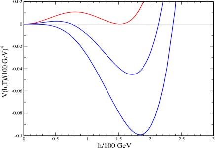
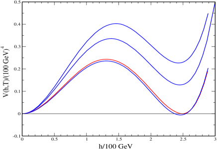
Figure 3: Effective potential around the EW phase transition, for $M_{h}=125$ GeV. Upper plot: $\zeta=0.8$ and $T=110.85$, 108.00 and 105.00 GeV, with $R\simeq 1.37$. Lower plot: Same for $\zeta=1.365$ and $T=50.00$, 40.00, 30.08 and 0 GeV with $R\simeq 8$.

We define $T_{c}$ as the critical temperature at which the origin and the non-trivial minimum at $\langle h(T_{c})\rangle$ become degenerate, calling its ratio $R\equiv\langle h(T_{c})\rangle/T_{c}$. The baryogenesis condition for non-erasure of the previously generated baryon asymmetry requires $R\stackrel{{\scriptstyle>}}{{{}_{\sim}}}1$ Bochkarev:1990gb . In general, identifying the critical temperature with the real tunneling temperature (which is smaller) underestimates $R$ so that our approximation provides a conservative estimate of the order parameter $R$. For a more detailed analysis see Ref. eqPRD .

We illustrate in Fig. 3 the behavior of the effective potential around the critical temperature for a fixed Higgs mass ($M_{h}=125$ GeV) and for two typical cases. In the upper plot we consider a case where the strength of the phase transition is only due to the thermal barrier from $S_{i}$ fields (with $\zeta=0.8$) with no $T=0$ barrier, leading to $R\simeq 1.37$. In the lower plot, with $\zeta=1.365$, the barrier persists all the way down to $T=0$ making the value of $R$ much larger ($R\simeq 8$). The dependence of $R$ with $\zeta$ for different values of $M_{h}$ is displayed in Fig. 4 where the strong enhancement in the values of $R$ produced inside the region where the barrier between the origin and the electroweak minima persists at $T=0$ is apparent (the square dots mark in each case the region beyond which there is a barrier at $T=0$). The answer to the general question of what is the upper bound on the Higgs mass to avoid baryon asymmetry washout depends on how large $\zeta$ can be, which in turn depends on the cutoff $\Lambda$. A low cutoff, e.g. $\Lambda\sim 1-10$ TeV, allows values of $\zeta$ up to $1.3-1.8$ while a higher cutoff $\Lambda\sim 10^{5}$ GeV would only allow values of $\zeta\stackrel{{\scriptstyle<}}{{{}_{\sim}}}1$.

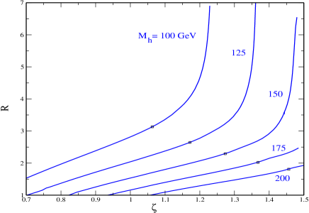
Figure 4: $R\equiv\langle h(T_{c})\rangle/T_{c}$ as a function of $\zeta$ for several values of $M_{h}$, as indicated.

A pending issue is how the baryon asymmetry is created (perhaps by the hidden sector) since within the SM the amount of CP violation, given by the CKM phase, is admittedly insufficient Gavela:1994dt (although a way out associated with physics solving the flavor problem at a high-scale was proposed in Berkooz:2004kx ). An interesting possibility from the low energy point of view is the appearance of CP-violating effective operators. For instance the dimension-six operator $g^{2}|H|^{2}F\tilde{F}/(32\pi^{2}\Lambda^{2})$ can generate the baryon-to-entropy ratio (for maximal CP violation) Dine:1990fj $n_{B}/s\sim 3.1\kappa\times 10^{-9}\left(T_{c}/\Lambda\right)^{2}$, where $\kappa\simeq 0.01-1$, which is roughly consistent with WMAP data for $\Lambda$ in the TeV range.

4. Conclusion. In this letter we have explored new and dramatic effects that a hidden sector, singlet under the SM gauge group, can have concerning electroweak symmetry breaking and electroweak baryogenesis. Completely new patterns for the Higgs potential and new ways of radiative breaking by dimensional transmutation are found, some of them indirectly leading to a very strong EW first order phase transition. For such a strong first-order phase transition the model can provide a strong signature in gravitational waves Randall:2006py . Moreover if the hidden sector has a global $U(1)$ symmetry that guarantees the stability of $S_{i}$-scalars (as we are assuming) and some subsector of it has a large invariant mass it can also provide good candidates for Dark Matter McDonald ; eqPRD .

- (1) B. Patt and F. Wilczek, [hep-ph/0605188].
- (2) R. Schabinger and J. D. Wells, Phys. Rev. D 72, 09300 (2005) [hep-ph/0509209]; M. Bowen, Y. Cui and J. Wells, [hep-ph/0701035].
- (3) M. J. Strassler and K. M. Zurek, [hep-ph/0604261]; [hep-ph/0605193]; M. J. Strassler, [hep-ph/0607160];
- (4) S. Chang, P. J. Fox and N. Weiner, JHEP 0608, 068 (2006) [hep-ph/0511250].
- (5) G. Burdman, Z. Chacko, H. S. Goh and R. Harnik, [hep-ph/0609152].
- (6) D. G. Cerdeño, A. Dedes and T. E. J. Underwood, JHEP 0609, 067 (2006) [hep-ph/0607157].
- (7) D. O’Connell, M. J. Ramsey-Musolf and M. B. Wise, [hep-ph/0611014].
- (8) J. R. Espinosa and J. F. Gunion, Phys. Rev. Lett. 82, 1084 (1999) [hep-ph/9807275]; O. Bahat-Treidel, Y. Grossman and Y. Rozen, [hep-ph/0611162].
- (9) K. A. Meissner and H. Nicolai, [hep-th/0612165]. This model is similar in spirit to ours when but considers one singlet with a non zero vacuum expectation value.
- (10) J.R. Espinosa, J. M. No and M. Quirós, to appear.
- (11) Similar effective Higgs couplings are used in J. A. Casas, J. R. Espinosa and M. Quirós, Phys. Lett. B 342, 171 (1995) [hep-ph/9409458]; Phys. Lett. B 382, 374 (1996) [hep-ph/9603227].
- (12) G. W. Anderson and L. J. Hall, Phys. Rev. D 45, 2685 (1992).
- (13) J. R. Espinosa and M. Quirós, Phys. Lett. B 305, 98 (1993) [hep-ph/9301285].
- (14) Although it is also possible in other models. See e.g. M. Pietroni, Nucl. Phys. B 402, 27 (1993) [hep-ph/9207227]; C. Grojean, G. Servant and J. D. Wells, Phys. Rev. D 71, 036001 (2005) [hep-ph/0407019].
- (15) A. I. Bochkarev, S. V. Kuzmin and M. E. Shaposhnikov, Phys. Rev. D 43, 369 (1991).
- (16) M. B. Gavela, P. Hernández, J. Orloff, O. Péne and C. Quimbay, Nucl. Phys. B 430, 382 (1994) [hep-ph/9406289].
- (17) M. Berkooz, Y. Nir and T. Volansky, Phys. Rev. Lett. 93, 051301 (2004) [hep-ph/0401012].
- (18) M. Dine, P. Huet, R. L. Singleton and L. Susskind, Phys. Lett. B 257, 351 (1991).
- (19) L. Randall and G. Servant, [hep-ph/0607158]; C. Grojean and G. Servant, [hep-ph/0607107].
- (20) J. McDonald, Phys. Rev. Lett. 88, 091304 (2002) [hep-ph/0106249].