A model for high-energy, small-angle pion-nucleus bremsstrahlung, $\pi^{-}+A\rightarrow\pi^{-}+\gamma+A$, is developed within the Glauber diffraction theory. Special attention is focussed on the possibility of measuring the pion polarisability in such reactions. That is the case under the Coulomb peak provided the bremsstrahlung photon carries practically all the energy of the incident pion. Only radiation from external legs is considered.

PACS: 13.40-f, 24.10.Ht, 25.80.Ht

1 Introduction

Consider a high-energy coherent nuclear production process

$$a+A\rightarrow a^{\star}+A$$

with quantum numbers exchanged those of the photon. Such a reaction can be initiated by a one-photon exhange, Coulomb production, or by strong interactions. The characteristic feature of Coulomb production is a very sharp peak near the forward direction. As energy increases the peak becomes sharper and at the same time moves towards smaller angles. As a consequence, it becomes possible to disentangle Coulomb and strong production. If the final state hadron $a^{\star}$ is a resonance the decay rate $\Gamma(a^{\star}\rightarrow a\gamma)$ can be determined. This was first noticed by Primakoff [1], and many radiative decay rates have been determined this way. A unified theoretical description of both strong and Coulomb production within the Glauber model was presented in ref. [2].

The final state hadron $a^{\star}$ need not be a resonance. It can also be a multiparticle state. In that case Coulomb production gives information on the cross section for the reaction $\gamma+a\rightarrow\gamma+a^{\star}$ [3]. An example is pionic Coulomb production or bremsstrahlung,

$$\pi^{-}+A\rightarrow\pi^{-}+\gamma+A$$

which is driven by low-energy Compton scattering $\gamma+\pi^{-}\rightarrow\gamma+\pi^{-}$. It has been suggested [4], that by studying pionic Coulomb production important information on the Compton amplitude can be extracted. The low-energy Compton scattering amplitude is a sum of two contributions, a structure-independent Thomson term, and a structure-dependent Rayleigh term. The latter is fixed by the pion polarisability, and could, under ideal circumstancies be determined in high-energy nuclear Coulomb production. An experiment with this aim has been performed [5], and a reasonable value for the pion polarisability was extracted.

We shall investigate pionic Coulomb production within the Glauber model [6]. In particular, we are interested in determining the nuclear form factors that accompany the various terms in the underlying Compton amplitude.

Our presentation is arranged as follows. First, we recall the theoretical description of low-energy pion Compton scattering. Then, we use this information to develop, in the Born approximation, the nuclear small-angle amplitude for pionic Coulomb production. Finally, we show how these expressions are changed when nuclear multiple scattering is taken into account. Coulomb as well as nuclear multiple scattering is considered.

2 Pion Compton scattering

The driving amplitude for pionic Coulomb production is the the low-energy pion Compton amplitude. It is important to understand the origin and structure of the various contributions to this amplitude since different sub amplitudes might lead to different form factors when embedded in the nucleus. That we need the low-energy amplitude can be understood by looking at the the reaction from a coordinate system where the initial pion is at rest and the nucleus runs past at high speed. Since we are in the Coulomb region the momentum transfer is extremely tiny and the kick to the pion consequently very gentle.

The Compton amplitude can be written as

$${\mathcal{M}}(\gamma(q_{1})\pi^{-}(p_{1})\rightarrow\gamma(q_{2})\pi^{-}(p_{2}))={\mathcal{M}}_{\mu\nu}\epsilon_{1}^{\mu}(q_{1})\epsilon_{2}^{\nu}(q_{2})\ .$$

Gauge invariance requires that, for real as well as virtual photons with $q^{2}\neq 0$, the Compton tensor satisfies

$${\mathcal{M}}_{\mu\nu}q_{1}^{\mu}={\mathcal{M}}_{\mu\nu}q_{2}^{\nu}=0\ .$$

We need the dominant contributions to the amplitude at small c.m. energies. They are the Born terms and the polarisability terms.

For pions there are three Born amplitudes described by the Feynman diagrams of fig. 1.

Figure 1: Born diagrams for pion Compton scattering.

Their sum is gauge invariant

$${\mathcal{M}}_{\mu\nu}^{B}=ie^{2}\left[2g_{\mu\nu}-\frac{(2p_{2}+q_{2})_{\nu}(2p_{1}+q_{1})_{\mu}}{2p_{2}\cdot q_{2}}-\frac{(2p_{1}-q_{2})_{\nu}(2p_{2}-q_{1})_{\mu}}{-2p_{1}\cdot q_{2}}\right].$$ (2.1)

This expression is correct also when $q_{1}^{2}\neq 0$, and that will be important for our applications. In the low-energy limit the amplitude ${\mathcal{M}}_{\mu\nu}^{B}$ reduces to the structure-independent Thompson term.

Terms quadratic in the photon energies are structure dependent, Rayleigh terms. They come from diagrams like

Figure 2: One-loop Feynman diagrams in chiral-Lagrangian theory.

In second order of the photon momenta we can construct two gauge invariant Compton tensors, which we choose to be

$${\mathcal{M}}_{\mu\nu}^{I}=ie^{2}\,\displaystyle{\frac{2m_{\pi}\beta_{\pi}}{\alpha}}\bigg{[}q_{1}\cdot q_{2}\,g_{\mu\nu}-q_{2\mu}q_{1\nu}\bigg{]}$$ (2.2)

with $\beta_{\pi}$ the magnetic polarisability, and

$$\begin{array}[]{rl}{\mathcal{M}}_{\mu\nu}^{II}=&ie^{2}\,\displaystyle{\frac{-2(\alpha_{\pi}+\beta_{\pi})}{m_{\pi}\alpha}}\bigg{[}p_{1}\cdot q_{1}p_{1}\cdot q_{2}\,g_{\mu\nu}+q_{1}\cdot q_{2}\,p_{1\mu}p_{1\nu}\\ &-p_{1}\cdot q_{1}\,q_{2\mu}p_{1\nu}-p_{1}\cdot q_{2}\,p_{1\mu}q_{1\nu}\bigg{]}\end{array}$$ (2.3)

with $\alpha_{\pi}$ the electric polarisability. The Compton amplitude is the sum of the above individual contributions, expressions (2.1), (2.2) and (2.3). Evaluated in the lab system (initial pion at rest) the Compton amplitude reads

$$\begin{array}[]{rl}{\mathcal{M}}=&i8\pi m_{\pi}\big{[}\displaystyle{-\frac{\alpha}{m_{\pi}}}\mbox{\boldmath{${\epsilon}$}}_{1}\cdot\mbox{\boldmath{${\epsilon}$}}_{2}\\ &+\alpha_{\pi}\omega_{1}\omega_{2}\mbox{\boldmath{${\epsilon}$}}_{1}\cdot\mbox{\boldmath{${\epsilon}$}}_{2}+\beta_{\pi}(\mbox{\boldmath{${q}$}}_{1}\times\mbox{\boldmath{${\epsilon}$}}_{1})\cdot(\mbox{\boldmath{${q}$}}_{2}\times\mbox{\boldmath{${\epsilon}$}}_{2})\big{]}\ .\end{array}$$

In ChPT one obtains in the one-loop order [7]

$$\alpha_{\pi^{\pm}}=-\beta_{\pi^{\pm}}=2.7\cdot 10^{-4}\ \mbox{\rm fm}^{3}.$$

In this order one has, $\alpha_{\pi^{\pm}}+\beta_{\pi^{\pm}}=0$, and we shall assume this relation throughout. Also two-loop contributions to the polarisabilities have been calculated [8], and found to be small. Therefore, we put ${\mathcal{M}}_{\mu\nu}^{II}=0.$ It is useful to introduce the dimensionless parameter

$$\lambda=\frac{\beta_{\pi^{\pm}}m_{\pi^{\pm}}^{3}}{\alpha}=-0.013\ .$$ (2.4)

There is no agreement on the experimental value of the polarisability so we shall use the value (2.4) as a guide in our deliberations.

3 Pionic bremsstrahlung: Born approximation

Pionic bremsstrahlung can be accompanied both by electromagnetic and strong interactions. We are interested in the region of small momentum transfers to the nucleus, and in particular the Coulomb region. This means that when the pion interaction with the nucleus is through a one-photon exchange, then the relevant Compton amplitude is a low-energy amplitude, as desired.

The kinematics of pionic bremsstrahlung is

$$\pi^{-}(p_{1})+A(p)\rightarrow\pi^{-}(p_{2})+\gamma(q_{2})+A(p^{\prime})\ .$$

Our interest is focussed on coherent high-energy interactions where the energies of the pions, as well as that of the radiated photon, are many GeV:s. Coherence demands that the transverse momenta $\mbox{\boldmath{${p}$}}_{2\bot}$ and $\mbox{\boldmath{${q}$}}_{2\bot}$ be much smaller than the inverse of the nuclear radius $R_{A}$, and as a consequence of the high energies, the longitudinal momentum transfer to the nucleus may be ignored. Thus, to a precision sufficient for the subsequent analysis we put

$$p_{1z}=p_{2z}+q_{2z}$$

with $z$ denoting the longitudinal direction. The energy transfer to the nucleus can likewise be ignored.

The one-photon exchange graph is pictured in fig. 3. The small blob in the

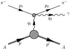
Figure 3: Born diagram for pionic bremsstrahlung.

graph represents the full pion-Compton amplitude; the large blob the photon-nucleus electromagnetic vertex. The pion charge is $-e$, the nuclear charge $Ze$, and the nucleus is treated as a spin-zero particle. With $q_{1}$ the virtual photon four-momentum, these assumptions lead to a Coulomb production amplitude

$${\mathcal{M}}_{C}=\frac{-i}{q_{1}^{2}}{\mathcal{M}}_{\mu\nu}(p_{2},q_{2};p_{1},q_{1})(-iZe)(p+p^{\prime})^{\mu}\epsilon_{2}^{\nu}\ .$$ (3.5)

Since the Compton tensor ${\mathcal{M}}_{\mu\nu}$ is gauge invariant we may also make the replacement $p+p^{\prime}=2p+q_{1}\rightarrow 2p$.

The expression for ${\mathcal{M}}_{C}$ is covariant and valid in all coordinate systems. We prefer to work in the lab system where the initial nucleus, of mass $M_{A}$, is at rest. Choosing a polarisation vector $\epsilon_{2}$ with vanishing time component, leads to

$$\begin{array}[]{rcl}{\mathcal{M}}_{C}&=&8i\pi M_{A}\,\displaystyle{\frac{-2Z\alpha}{q_{1}^{2}}}\,e\bigg{[}\left(\frac{E_{1}\mbox{\boldmath{${p}$}}_{2}\cdot\mbox{\boldmath{${\epsilon}$}}_{2}}{p_{2}\cdot q_{2}}-\frac{E_{2}\mbox{\boldmath{${p}$}}_{1}\cdot\mbox{\boldmath{${\epsilon}$}}_{2}}{p_{1}\cdot q_{2}}\right)\\ &&\\ &&\qquad\qquad\qquad\qquad\qquad+\displaystyle{\frac{\lambda\omega_{2}}{m_{\pi}^{2}}}\,(\mbox{\boldmath{${p}$}}_{2}-\mbox{\boldmath{${p}$}}_{1})\cdot\mbox{\boldmath{${\epsilon}$}}_{2}\bigg{]}\ .\end{array}$$ (3.6)

Here, the first two terms originate from the Compton Born terms of eq.(2.1). The $g_{\mu\nu}$ Born term does not contribute to ${\mathcal{M}}_{C}$. Instead, the first term of (3.6) originates from the middle term of eq.(2.1) and represents a pion-nucleus elastic scattering step followed by a pionic bremsstrahlung step. Similarly, the second term of (3.6) originates from the last term of eq.(2.1) and represents a pionic bremsstrahlung step followed by a pion-nucleus elastic scattering step.

The last term of (3.6), finally, is generated by the polarisability contribution, eq.(2.2), to the Compton amplitude. In this term the radiated and exchanged photons are attached to the same vertex. The second polarisability contribution, eq.(2.3), vanishes since we presume $\alpha_{\pi}+\beta_{\pi}=0$.

Pionic bremsstrahlung from the external pion legs can also occur in nuclear interactions, as depicted in fig. 4. For $\pi^{-}$ scattering, with $q_{1}=p-p^{\prime}$

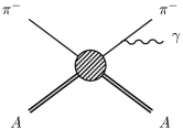
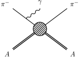
Figure 4: Pion bremsstrahlung in nuclear scattering.

the four-momentum transfer to the nucleus, as above, the nuclear contribution to pionic bremsstrahlung reads

$${\mathcal{M}}_{N}=e\bigg{[}-\frac{\epsilon_{2}\cdot p_{2}}{p_{2}\cdot q_{2}}{\mathcal{M}}_{\pi A}(s_{1},q_{1})+\frac{\epsilon_{2}\cdot p_{1}}{p_{1}\cdot q_{2}}{\mathcal{M}}_{\pi A}(s_{2},q_{1})\bigg{]}\ .$$ (3.7)

Here, ${\mathcal{M}}_{\pi A}(s,q)$ is the elastic pion-nucleus scattering amplitude at energy $s$ and momentum transfer $q$. The nuclear scattering steps occur with the same momentum transfer. In the first term of (3.7) the pion-nucleus scattering occurs after the photon is radiated, and the amplitude should therefore be evaluated at energy $s_{2}=(p_{2}+p^{\prime})^{2}$. Similarly, the pion-nucleus amplitude of the second term of eq.(3.7) is evaluated at $s_{1}=(p_{1}+p)^{2}$. To insure gauge invariance of ${\mathcal{M}}_{N}$ one could, e.g., evaluate the pion-nucleus amplitudes at the same energy $s$. The alternative is to add an appropriate counter term arising from internal radiation. We shall not do so, however, but shall take the amplitude (3.7) as it stands. The error committed is probably negligible.

The pion-nucleus amplitude ${\mathcal{M}}_{\pi A}(s,q)$ is related to the pion-nucleus elastic scattering amplitude in the lab system, $F_{N}(E,\mbox{\boldmath{${q}$}})$, through

$${\mathcal{M}}_{\pi A}(s,q)=8i\pi M_{A}\,F_{N}(E,\mbox{\boldmath{${q}$}})$$ (3.8)

with $E$ the pion lab energy. The amplitude $F_{N}(E,\mbox{\boldmath{${q}$}})$ depends only on the transverse part $\mbox{\boldmath{${q}$}}_{\bot}$ of ${q}$.

In our application we are in an energy region where the pion-nucleus total cross section $\sigma_{\pi A}$ may be considered independent of energy. If in addition, we specialise to the region of Coulomb production the dependence on momentum transfer can be ignored, and a simple energy dependence emerges

$$F_{N}(E,0)=\frac{ik}{4\pi}\sigma_{\pi A}(1-i\alpha_{\pi A})\equiv\frac{ik}{4\pi}\sigma_{\pi A}^{\prime}\ .$$ (3.9)

Since at high energies there is no distinction between $k$ and $E$ we can write the nuclear bremsstrahlung contribution as

$${\mathcal{M}}_{N}=8i\pi M_{A}\,\frac{ie\sigma_{\pi A}^{\prime}}{4\pi}\bigg{[}\frac{E_{1}\mbox{\boldmath{${\epsilon}$}}_{2}\cdot\mbox{\boldmath{${p}$}}_{2}}{p_{2}\cdot q_{2}}-\frac{E_{2}\mbox{\boldmath{${\epsilon}$}}_{2}\cdot\mbox{\boldmath{${p}$}}_{1}}{p_{1}\cdot q_{2}}\bigg{]}\ .$$ (3.10)

The factor inside the brackets is identical to the corresponding factor in eq.(3.6) describing radiation from the external legs.

The strong pion-nucleus amplitude ${\mathcal{M}}_{\pi A}$ is conveniently calculated in the Glauber model. Further details below.

4 Elastic Coulomb scattering

At this point it is useful to recall the eikonal description of elastic Coulomb scattering. The Coulomb potential for $\pi^{-}$-nucleus scattering is

$$V_{C}(\mbox{\boldmath{${r}$}})=-\frac{Z\alpha}{r}$$ (4.11)

and the scattering amplitude in the Born approximation

$$f_{C}(E,\mathbf{q})=-\frac{E}{2\pi}\int\textrm{d}^{3}x\,e^{-i\mathbf{q}\cdot\mathbf{x}}\,V_{C}(\mathbf{r})=\frac{2Z\alpha E}{\mathbf{q}^{2}}$$ (4.12)

with the momentum transfer $\mbox{\boldmath{${q}$}}=\mbox{\boldmath{${k}$}}^{\prime}-\mbox{\boldmath{${k}$}}$. In reality, at high energies the momentum tranfer is transverse so that $\mathbf{q}=\mathbf{q}_{\bot}$.

Elastic Coulomb scattering to all orders in the fine-structure constant is exactly reproduced by the eikonal approximation

$$f_{C}(E,\mathbf{q})=\frac{ik}{2\pi}\int\textrm{d}^{2}b\,e^{-i\mathbf{q}\cdot\mathbf{b}}[1-e^{i\chi_{C}(\mathbf{b})}]$$ (4.13)

with the point-like Coulomb phase function

$$\chi_{C}(\mathbf{b}) = -\eta\ln(b/2a)$$ (4.14)

$$\eta = 2Z\alpha/v\ .$$ (4.15)

Here, $a$ is a cut-off parameter introduced in order to make the phase function finite. The Coulomb potential is cut off at a radius $r=a$.

At high energies there is no distinction between $E$ and $k$, and $v=1$. A straightforward integration gives the well-known result

$$f_{C}(E,\mathbf{q}) = \frac{2Z\alpha E}{\mathbf{q}^{2}}\exp[i\sigma_{\eta}+i\eta\ln(aq)]$$ (4.16)

$$\sigma_{\eta} = 2\arg\Gamma(1-i\eta/2)\ .$$ (4.17)

A thorough description of Coulomb scattering in the eikonal approximation can be found in [6], but also [9] contains useful information. For an extended charge distribution the phase-shift function takes the form

$$\chi_{C}(b)=-\eta\left[\ln(b/2a)+2\pi\int_{b}^{\infty}T(b^{\prime})\ln(b^{\prime}/b)b^{\prime}\textrm{d}b^{\prime}\right]$$ (4.18)

where the target-thickness function $T(b)$ corresponds to a nuclear charge-density distribution normalised to unity.

In the real world pions obey the Klein-Gordon equation which contains one term that is linear in the Coulomb potential $V_{C}(\mbox{\boldmath{${r}$}})$, and one which is quadratic. The above applies to the linear term. The quadratic term leads to corrections that can be expanded in powers of $\sin\theta/2=q/2k$. For a point charge in the Klein-Gordon case [10]

$$f_{C}^{KG}(E,\mathbf{q}) = f_{C}(E,\mathbf{q})\left\{1+\frac{\pi(Z\alpha)^{2}e^{i\sigma_{1}}}{\eta}\frac{q}{2k}+\ldots\right\}$$ (4.19)

$$\sigma_{1} = 2[\arg\Gamma(\mbox{${\textstyle\frac{1}{2}}$}+i\eta/2)-\arg\Gamma(1+i\eta/2)]\ .$$ (4.20)

A few of the higher order corrections have also been evaluated [11]. The important point for us is that we consider the very small angular region where the correction terms safely can be neglected. The corrections due to the extension of the nuclear charge distribution are negligible as well.

5 Pionic bremsstrahlung: eikonal approximation

The Born amplitudes are strongly modified by nuclear multiple scattering, a modification most easily calculated in the eikonal approximation. But first a remark on the four-momentum transfer to the nucleus, $q_{1}$. Its time component can always be neglected, so that

$$-q_{1}^{2}=\mathbf{q}_{1}^{2}=\mathbf{q}_{1\bot}^{2}+q_{1z}^{2}\ .$$ (5.21)

The longitudinal momentum transfer $-q_{1z}$ is tiny and can be replaced by its minimum value

$$q_{min}=\frac{m^{2}\omega_{2}}{2E_{1}E_{2}}$$ (5.22)

but we shall start by neglecting $q_{1z}$ altogether and later return to the modifications dictated by its presence.

In the Coulomb-induced bremsstrahlung amplitude (3.6), Coulomb scattering in the one-photon approximation is described by the factor

$$\frac{2Z\alpha E_{1}}{\mathbf{q}_{1\bot}^{2}}\ .$$ (5.23)

The very first term of (3.6) represents Coulomb scattering followed by bremsstrahlung. To include multiple Coulomb scattering we add all diagrams with multiple-photon exchanges between the pion and the nucleus. If all these exchanges occur before the bremsstrahlung step then we simply replace the Born amplitude (5.23) by the full Coulomb amplitude of eq.(4.13). The contributions from the diagrams where radiation occurs from an intermediate pion line, i.e., when we have photon exchanges both before and after the radiation step, cancel to a large extent. Therefore, diagrams with radiation from internal lines are ignored. The corresponding argument applies to the second term of (3.6) as well.

The nuclear-induced bremsstrahlung amplitude (3.7), must be similarly modified. The pion can radiate when between two nucleon collisions, if we view the nuclear interaction as caused by multiple interactions between the pion and the nucleons of the nucleus. Again, the contributions from the internal radiation diagrams cancel when summed.

A further generalisation is to include Coulomb and nuclear exchanges simultaneously. Since internal radiation diagrams are ignored we get

$${\mathcal{M}}_{rad}=8\pi iM_{A}e\bigg{[}-\displaystyle{\frac{E_{2}\mbox{\boldmath{${p}$}}_{1}\cdot\mbox{\boldmath{${\epsilon}$}}_{2}}{p_{1}\cdot q_{2}}}+\displaystyle{\frac{E_{1}\mbox{\boldmath{${p}$}}_{2}\cdot\mbox{\boldmath{${\epsilon}$}}_{2}}{p_{2}\cdot q_{2}}}\bigg{]}{\mathcal{F}}_{rad}(\mbox{\boldmath{${q}$}}_{1\bot})\ .$$ (5.24)

The factor ${\mathcal{F}}_{rad}(\mbox{\boldmath{${q}$}}_{\bot})$ is the pion-nucleus scattering amplitude, including both its Coulomb and nuclear interactions. In the Glauber model

$${\mathcal{F}}_{rad}(\mbox{\boldmath{${q}$}}_{\bot})=\frac{iv}{2\pi}\int\textrm{d}^{2}b\,e^{-i\mathbf{q}_{\bot}\cdot\mathbf{b}}\left(1-e^{i(\chi_{C}(\mathbf{b})+\chi_{N}(\mathbf{b}))}\right)$$ (5.25)

with the momentum transfer $\mathbf{q}_{\bot}$ in the impact parameter plane. The function ${\mathcal{F}}_{rad}(\mbox{\boldmath{${q}$}}_{\bot})$ is energy independent, providing we can put $v=1$ and neglect the energy dependence of the pion-nucleus potentials. The phase-shift functions are related to the corresponding potentials, whether Coulomb or nuclear, through

$$\chi(\mathbf{b})=\frac{-1}{v}\int_{-\infty}^{\infty}\textrm{d}z\,V(\mathbf{b},z)\ .$$ (5.26)

We can, in a well-known fashion, decompose ${\mathcal{F}}_{rad}(\mbox{\boldmath{${q}$}})$ into a purely Coulomb and a Coulomb-distorted nuclear amplitude by writing

$${\mathcal{F}}_{rad}(\mbox{\boldmath{${q}$}}_{\bot}) = \frac{iv}{2\pi}\int\textrm{d}^{2}b\,e^{-i\mathbf{q}_{\bot}\cdot\mathbf{b}}\left(1-e^{i\chi_{C}(\mathbf{b})}\right)$$ (5.27)

$$+\frac{iv}{2\pi}\int\textrm{d}^{2}b\,e^{-i\mathbf{q}_{\bot}\cdot\mathbf{b}}e^{i\chi_{C}(\mathbf{b})}\left(1-e^{i\chi_{N}(\mathbf{b})}\right)$$

$$\equiv [f_{C}(E,\mbox{\boldmath{${q}$}}_{\bot})+f_{N}(E,\mbox{\boldmath{${q}$}}_{\bot})]/E\ .$$

The analytic expression of the Coulomb amplitude $f_{C}(E,\mbox{\boldmath{${q}$}}_{\bot})$ for a point charge distribution is given in eq.(4.16).

The polarisation-induced bremsstrahlung amplitude is the third term of (3.6). Before proceeding we note the identities $(\mbox{\boldmath{${p}$}}_{2}-\mbox{\boldmath{${p}$}}_{1})\cdot\mbox{\boldmath{${\epsilon}$}}_{2}=\mbox{\boldmath{${q}$}}_{1}\cdot\mbox{\boldmath{${\epsilon}$}}_{2}$ and

$${\frac{2Z\alpha}{\mbox{\boldmath{${q}$}}_{1}^{2}}}\,\mbox{\boldmath{${q}$}}_{1}\cdot\mbox{\boldmath{${\epsilon}$}}_{2}=\displaystyle{\frac{i}{2\pi}}\int\textrm{d}^{3}r\,e^{-i\mathbf{q}_{1}\cdot\mathbf{r}}\,\mbox{\boldmath{${\epsilon}$}}_{2}\cdot\mbox{\boldmath{${\nabla}$}}V_{C}(\mbox{\boldmath{${r}$}})\ .$$ (5.28)

The polarisation potential is hence proportional to the gradient of the Coulomb potential. We now replace the plane waves of the Born approximation by distorted waves, assume energy-independent pion-nucleus potentials and neglect the longitudinal momentum transfer $q_{1z}$. Introducing phase-shift functions instead of potentials leads to the energy-independent expression, $v=v_{1}=v_{2}$,

$${\frac{-iv}{2\pi}}\int\textrm{d}^{2}b\,e^{-i\mathbf{q}_{1\bot}\cdot\mathbf{b}}\,\mbox{\boldmath{${\epsilon}$}}_{2}\cdot\mbox{\boldmath{${\nabla}$}}\chi_{C}(\mathbf{b})e^{i(\chi_{C}(\mathbf{b})+\chi_{N}(\mathbf{b}))}\ .$$ (5.29)

With help of the identity

$$e^{i(\chi_{C}(\mathbf{b})+\chi_{N}(\mathbf{b}))}=e^{i\chi_{C}(\mathbf{b})}-e^{i\chi_{C}(\mathbf{b})}(1-e^{i\chi_{N}(\mathbf{b})})$$ (5.30)

we can easily isolate a purely Coulombic term from a rest term which involves also nuclear effects. After partial integration of the first term of (5.30) and an angular integration of the second one, expression (5.29) can be written as

$$\mathbf{q}_{1\bot}\cdot\mbox{\boldmath{${\epsilon}$}}_{2}{\mathcal{F}}_{pol}(\mbox{\boldmath{${q}$}}_{1\bot})\ .$$ (5.31)

The energy-independent form factor ${\mathcal{F}}_{pol}(\mbox{\boldmath{${q}$}}_{1\bot})$ is

$${\mathcal{F}}_{pol}(\mbox{\boldmath{${q}$}}_{\bot})=[f_{C}(E,\mathbf{q}_{\bot})+f_{P}(E,\mathbf{q}_{\bot})]/E$$ (5.32)

with $f_{C}(E,\mathbf{q}_{\bot})$ the elastic Coulomb scattering amplitude and the new amplitude $f_{P}(E,\mathbf{q}_{\bot})$ defined by, $q_{\bot}=\|\mathbf{q}_{\bot}\|$,

$$f_{P}(E,\mathbf{q}_{\bot})=k\int_{0}^{\infty}b^{2}\textrm{d}b\,\frac{J_{1}(q_{\bot}b)}{q_{\bot}b}\frac{\textrm{d}\chi_{C}(b)}{\textrm{d}b}e^{i\chi_{C}(b)}(1-e^{i\chi_{N}(b)})\ .$$ (5.33)

The last factor of the integrand guarantees that the integrand vanishes outside the nuclear mass distribution. From the definition of the Coulomb phase for extended charge distributions, eq.(4.18), we derive

$$\frac{\textrm{d}\chi_{C}(b)}{\textrm{d}b}=-2\pi\eta\frac{1}{b}\int_{0}^{b}b^{\prime}\textrm{d}b^{\prime}\,T(b^{\prime})\ .$$ (5.34)

The result of all this is a polarisation contribution to the bremsstrahlung amplitude

$${\mathcal{M}}_{pol}=8\pi ieM_{A}\bigg{[}\frac{\lambda}{m_{\pi}^{2}}\,\omega_{2}\mathbf{q}_{1}\cdot\mbox{\boldmath{${\epsilon}$}}_{2}\bigg{]}{\mathcal{F}}_{pol}(\mbox{\boldmath{${q}$}}_{1\bot})\ .$$ (5.35)

To get the complete ${\mathcal{M}}$-amplitude we add the amplitude ${\mathcal{M}}_{rad}$ representing radiation from external legs;

$${\mathcal{M}} = 8\pi ieM_{A}\bigg{\{}\big{[}-\displaystyle{\frac{E_{2}\mbox{\boldmath{${p}$}}_{1}\cdot\mbox{\boldmath{${\epsilon}$}}_{2}}{p_{1}\cdot q_{2}}}+\displaystyle{\frac{E_{1}\mbox{\boldmath{${p}$}}_{2}\cdot\mbox{\boldmath{${\epsilon}$}}_{2}}{p_{2}\cdot q_{2}}}\big{]}{\mathcal{F}}_{rad}(\mbox{\boldmath{${q}$}}_{1\bot})$$ (5.36)

$$\quad\quad+\big{[}\frac{\lambda}{m_{\pi}^{2}}\,\omega_{2}\mathbf{q}_{1}\cdot\mbox{\boldmath{${\epsilon}$}}_{2}\big{]}{\mathcal{F}}_{pol}(\mbox{\boldmath{${q}$}}_{1\bot})\bigg{\}}\ .$$

So far we have kept the cut-off parameter $a$ of the Coulomb potential. This was intentional. We now remove the dependence on this parameter by removing a phase factor common to all amplitudes. This is conventionally done so that the Coulomb phase in the integrand of the nuclear amplitude, $f_{N}(E,\mbox{\boldmath{${q}$}}_{\bot})$ eq.(5.27), varies as slowly as possibly over the domain of integration. Since the main contribution comes from a region close to the nuclear rim, this goal is achieved by setting $2a=R_{u}$ in eq.(4.18). Here, $R_{u}$ is the equivalent radius of the uniform nuclear mass distribution.

Let us now return to the question of the longitudinal momentum transfer, $q_{min}$. In the nuclear and polarisation amplitudes, eqs (5.27) and (5.33), the integration is over the nuclear region, which has a finite extension. Since $q_{min}R_{u}\ll 1$ all dependence on $q_{min}$ can be ignored. Extracting appropriate phase factors we may write, with $q_{\bot}=\|\mathbf{q}_{\bot}\|$,

$$f_{N}(E,\mathbf{q}_{\bot}) = ike^{i\delta_{B}}\int b\textrm{d}b\,J_{0}(q_{\bot}b)\left(1-e^{i\chi_{N}(b)}\right)$$ (5.37)

$$f_{P}(E,\mathbf{q}_{\bot}) = ke^{i\delta_{B}^{\prime}}\int_{0}^{\infty}b^{2}\textrm{d}b\,\frac{J_{1}(q_{\bot}b)}{q_{\bot}b}\frac{\textrm{d}\chi_{C}(b)}{\textrm{d}b}(1-e^{i\chi_{N}(b)})$$ (5.38)

for the nuclear and polarisation amplitudes. The Bethe phases $\delta_{B}$ and $\delta_{B}^{\prime}$ need not be factorised as indicated. The original integrations could also have been carried out.

The pure Coulomb amplitude is more of a problem. In the Born approximation, as layed out in eq.(3.5), the Coulomb denominator contains the longitudinal momentum transfer through $\mathbf{q}_{1}^{2}=\mathbf{q}_{1\bot}^{2}+q_{min}^{2}$. When $q_{\bot}\gg q_{min}$ the dependence on $q_{min}$ can safely be ignored, but under the Coulomb peak, where $q_{\bot}\approx q_{min}$ that is not possible. A subsequent question is then how the nuclear form factor depends on $q_{min}$. This question has not yet been resolved analytically. Of course, the scattering amplitude can be calculated numerically, but until we have done so we suggest the point-charge Coulomb amplitude be chosen as

$$f_{C}(E,\mathbf{q}_{\bot})=\frac{2Z\alpha E}{\mathbf{q}_{\bot}^{2}+q_{min}^{2}}\,\exp[i\sigma_{\eta}+i\eta\ln(q_{\bot}R_{u}/2)]\ .$$ (5.39)

The form factor for extended charge distributions can, as is necessary for large momentum transfers, be calculated as in ref.[9].

6 Cross sections

The cross section distribution in the lab system is

$$\textrm{d}\sigma=\frac{1}{4p_{1}M_{A}}\left|{\mathcal{M}}\right|^{2}{\rm dLips}$$ (6.40)

where $p_{1}$ is the incident pion lab momentum. The Lorentz-invariant phase space is as always

$${\rm dLips} = (2\pi)^{4}\delta(p_{1}+p_{A}-p_{2}-q_{2}-p_{A}^{\prime})\frac{\textrm{d}^{3}p_{A}^{\prime}}{(2\pi)^{3}2E_{A}^{\prime}}\frac{\textrm{d}^{3}p_{2}}{(2\pi)^{3}2E_{2}}\frac{\textrm{d}^{3}q_{2}}{(2\pi)^{3}2\omega_{2}}$$ (6.41)

$$= \frac{1}{16\pi M_{A}}\frac{\textrm{d}^{2}p_{2\bot}}{(2\pi)^{2}}\frac{\textrm{d}^{2}q_{2\bot}}{(2\pi)^{2}}\frac{\textrm{d}q_{2z}}{p_{2z}q_{2z}}\ .$$

The pion propagators of eq.(5.36) can be rewritten as

$$p_{1}\cdot q_{2} = \frac{1}{2x}\left[\mathbf{q}_{2\bot}^{2}+x^{2}m_{\pi}^{2}\right]$$ (6.42)

$$p_{2}\cdot q_{2} = \frac{1}{2x^{\prime}}\left[(\mathbf{q}_{2\bot}-x^{\prime}\mathbf{p}_{2\bot})^{2}+x^{\prime 2}m_{\pi}^{2}\right]$$ (6.43)

with the parameters

$$x = \frac{q_{2z}}{p_{1}}=\frac{\omega_{2}}{E_{1}}$$ (6.44)

$$x^{\prime} = \frac{q_{2z}}{p_{2z}}=\frac{\omega_{2}}{E_{2}}=\frac{x}{1-x}\ .$$ (6.45)

The matrix element in eq.(5.36) can be further simplified. Since the polarisation vector $\mbox{\boldmath{${\epsilon}$}}_{2}$ lies in the plane orthogonal to $\mbox{\boldmath{${q}$}}_{2}$, the scalar products with the polarisation vector can be replaced by

$$\mbox{\boldmath{${p}$}}_{1}\cdot\mbox{\boldmath{${\epsilon}$}}_{2} = -\frac{1}{x}\,\mbox{\boldmath{${q}$}}_{2\bot}\cdot\mbox{\boldmath{${\epsilon}$}}_{2}$$ (6.46)

$$\mbox{\boldmath{${p}$}}_{2}\cdot\mbox{\boldmath{${\epsilon}$}}_{2} = (\mbox{\boldmath{${p}$}}_{2\bot}-\frac{1}{x^{\prime}}\,\mbox{\boldmath{${q}$}}_{2\bot})\cdot\mbox{\boldmath{${\epsilon}$}}_{2}$$ (6.47)

$$(\mbox{\boldmath{${p}$}}_{2}-\mbox{\boldmath{${p}$}}_{1})\cdot\mbox{\boldmath{${\epsilon}$}}_{2} = \mbox{\boldmath{${q}$}}_{1\bot}\cdot\mbox{\boldmath{${\epsilon}$}}_{2}\ ,$$ (6.48)

where perpendicular still means perpendicular to the incident pion direction. The new expression for the matrix element becomes more transparent

$${\cal M} = 16\pi ieM_{A}\left[\bigg{\{}\frac{E_{2}\mathbf{q}_{2\bot}}{\mathbf{q}_{2\bot}^{2}+x^{2}m_{\pi}^{2}}-\frac{E_{1}(\mathbf{q}_{2\bot}-x^{\prime}\mathbf{p}_{2\bot})}{(\mathbf{q}_{2\bot}-x^{\prime}\mathbf{p}_{2\bot})^{2}+x^{\prime 2}m_{\pi}^{2}}\bigg{\}}{\mathcal{F}}_{rad}(\mbox{\boldmath{${q}$}}_{1\bot})\right.$$ (6.49)

$$\left.\quad\quad+\frac{\lambda}{2}\frac{\omega_{2}\mathbf{q}_{1\bot}}{m_{\pi}^{2}}\,{\mathcal{F}}_{pol}(\mbox{\boldmath{${q}$}}_{1\bot})\right]\cdot\mbox{\boldmath{${\epsilon}$}}_{2}$$

and the summation over the photon polarisation directions embarrasingly trivial

$$\sum\left|{\cal M}\right|^{2} = 64(2\pi)^{2}e^{2}M_{A}^{2}$$ (6.50)

$$\times\left|\left[\frac{E_{2}\mathbf{q}_{2\bot}}{\mathbf{q}_{2\bot}^{2}+x^{2}m_{\pi}^{2}}-\frac{E_{1}(\mathbf{q}_{2\bot}-x^{\prime}\mathbf{p}_{2\bot})}{(\mathbf{q}_{2\bot}-x^{\prime}\mathbf{p}_{2\bot})^{2}+x^{\prime 2}m_{\pi}^{2}}\right]\right.{\mathcal{F}}_{rad}(\mbox{\boldmath{${q}$}}_{1\bot})$$

$$\left.\quad\quad+\frac{\lambda}{2}\frac{\omega_{2}\mathbf{q}_{1\bot}}{m_{\pi}^{2}}\,{\mathcal{F}}_{pol}(\mbox{\boldmath{${q}$}}_{1\bot})\right|^{2}$$

We recall that $\mbox{\boldmath{${q}$}}_{1}$ is the momenum transfer to the nucleus and

$$\mbox{\boldmath{${q}$}}_{1}=\mbox{\boldmath{${q}$}}_{2}+\mbox{\boldmath{${p}$}}_{2}$$ (6.51)

with $\mbox{\boldmath{${p}$}}_{2}$ the momentum of the final state pion and $\mbox{\boldmath{${q}$}}_{2}$ the momentum of the final state photon. In eq.(6.50) only the dependence on $\mbox{\boldmath{${q}$}}_{1\bot}$ is indicated. The longitudinal component is fixed by the relation

$$-q_{1z}=\frac{1}{2p_{1}}[2p_{2}\cdot q_{2}+\mbox{\boldmath{${q}$}}_{1\bot}^{2}]\ .$$ (6.52)

For all practical purposes it can be replaced by its value in the forward direction, $-q_{1z}=q_{min}$, with $q_{min}$ as given by eq.(5.22). As a consequence, the denominator $\mbox{\boldmath{${q}$}}_{1}^{2}=\mbox{\boldmath{${q}$}}_{1\bot}^{2}+q_{1z}^{2}$ of the Coulomb amplitude never vanishes. However, the factor multiplying the form factor ${\mathcal{F}}_{rad}$ in eq.(6.50) vanishes in the forward direction, since there $\mbox{\boldmath{${p}$}}_{1}\cdot\mbox{\boldmath{${\epsilon}$}}_{2}=\mbox{\boldmath{${p}$}}_{2}\cdot\mbox{\boldmath{${\epsilon}$}}_{2}=0$.

The cross section distribution is dominated by the first term of eq.(6.50) which is multiplied by the form factor ${\mathcal{F}}_{rad}$. The second term is proportional to the polarisability parameter $\lambda$ and the form factor ${\mathcal{F}}_{pol}$ and is generally smaller. Since ${\mathcal{F}}_{rad}$ is exactly the amplitude we encounter in elastic pion-nucleus scattering, this observation allows us to distinguish three regions, characterised by increasing values of the momentum transfer:

1. dominance of Coulomb bremsstrahlung

2. competition between Coulomb and nuclear bremsstrahlung

3. dominance of nuclear bremsstrahlung

In order to localise the proper Coulomb region we first localise the overlap region where Coulomb and nuclear contributions are of similar size. That happens when in the form factor ${\cal F}_{rad}$, eq.(5.27), the Coulomb $f_{C}$ and nuclear $f_{N}$ amplitudes are equal in size. This, according to eq.(8.65), is roughly the case when

$$\frac{2Z\alpha}{\mbox{\boldmath{${q}$}}_{1\bot}^{2}}=\frac{1}{2}R_{u}^{2}\ .$$ (6.53)

Putting $Z=A/2$ as a further approximation gives

$$\mbox{\boldmath{${q}$}}_{1\bot}^{2}\approx\frac{2\alpha}{r_{0}^{2}}A^{1/3}=0.5\cdot 10^{-3}A^{1/3}\quad{\rm(GeV/c)}^{2}\ .$$ (6.54)

Consequently, in the transition region we have for a typical nucleus $|t|\approx 10^{-3}$ (GeV/c)²; in the Coulomb-dominated region $|t|\approx 10^{-4}$ (GeV/c)²; and in the nuclear-dominated region $|t|\approx 10^{-2}$ (GeV/c)².

In the form factor ${\mathcal{F}}_{pol}$ the nuclear contribution $f_{P}$ is substantially smaller than the corresponding $f_{N}$ in ${\mathcal{F}}_{rad}$ and would thus need larger momentum transfers to make itself noticed. For Cu the ratio $|f_{P}(E,0)/f_{N}(E,0)|=0.12$ derived from the formulae in the Appendix, supports this statement.

There are kinematic variables, beside those chosen above, that are of fundamental interest, e.g.,

$$t = q_{1}^{2}$$ (6.55)

$$s = (p_{2}+q_{2})^{2}$$ (6.56)

$$\Delta = (p_{2}-p_{1})^{2}$$ (6.57)

which relate to properties of the underlying pion-Compton scattering process. In fact, $t$ is the squared momentum transfer to the nucleus, but also the squared mass of the virtual photon; $s$ is the square of the c.m. energy and $\Delta$ the squared momentum transfer in the pion-Compton scattering process. A simple calculation ends in the results

$$t = -\mbox{\boldmath{${q}$}}_{1\bot}^{2}-\left(\frac{\omega_{2}m_{\pi}}{2E_{1}E_{2}}\right)^{2}m_{\pi}^{2}$$ (6.58)

$$s = \frac{E_{1}}{E_{2}}m_{\pi}^{2}+\frac{1}{x^{\prime}}(\mathbf{q}_{2\bot}-x^{\prime}\mathbf{p}_{2\bot})^{2}$$ (6.59)

$$\Delta = -\frac{E_{1}}{E_{2}}\left[\mathbf{p}_{2\bot}^{2}+x^{2}m_{\pi}^{2}\right]\ .$$ (6.60)

From the expression for $s$ we conclude that in the Coulomb region the Compton scattering takes place at a lab energy of

$$\omega_{lab}=\mbox{${\textstyle\frac{1}{2}}$}x^{\prime}m_{\pi}\ .$$

Similarly, from the expression for $\Delta$ we conclude that the scattering angle in the pion-Compton c.m. system is $\theta_{cm}=90^{\circ}$, and in the lab system

$$\cos\theta_{lab}=-\frac{E_{1}-E_{2}}{E_{1}+E_{2}}=-\frac{x}{2-x}\ .$$

When $x^{\prime}$ is large, which is an interesting region, then $\omega_{lab}$ is also large, and one can legitimately ask where our basic amplitude for the Compton process breaks down.

Finally, there is the question of region of applicability of the model described above. It is commonly stated that the radiation from the external legs dominates as long as the propagator denominators, eqs (6.42) and (6.43), are of order $m_{\pi}^{2}$ or smaller. Our formulae should therefore work well into the nuclear region. A quantification of this statement would mean estimating diagrams where the photon is radiated from internal lines. We leave that investigation to a future paper.

7 Under the spell of the Coulomb peak

Pionic bremsstrahlung at very small momentum transfers, i.e. in the Coulomb region, is of special interest since it is there one can hope to extract the pion polarisability.

In the Coulomb region the transverse momentum transfers are so small they can safely be neglected in the propagators of eqs (6.42) and (6.43). Furthemore, as explained above, in this region the Coulomb contributions dominate the form factors ${\mathcal{F}}_{rad}$ and ${\mathcal{F}}_{pol}$, and both may be replaced by $f_{C}(E,\mbox{\boldmath{${q}$}}_{\bot})/E$ from eq.(5.39). After some straightforward simplifications we get the cross section distribution

$$\frac{\textrm{d}\sigma}{\textrm{d}^{2}q_{2\bot}\textrm{d}^{2}p_{2\bot}\textrm{d}x}=\frac{4Z^{2}\alpha^{3}}{\pi^{2}m_{\pi}^{4}}\Bigg{[}\frac{\mbox{\boldmath{${q}$}}_{1\bot}^{2}}{(\mbox{\boldmath{${q}$}}_{1\bot}^{2}+q_{min}^{2})^{2}}\Bigg{]}\Bigg{[}\frac{1-x}{x^{3}}\left(1+\frac{\lambda x^{2}}{2(1-x)}\right)^{2}\Bigg{]}$$ (7.61)

with $x=\omega_{2}/E_{1}$ from eq.(6.44).

The factor inside the first pair of brackets is typical for Coulomb production. It has the Coulomb propagator, with the minimum momentum transfer, but due to the numerator it vanishes in the forward direction. This last property can readily be seen from expression (3.6). In the forward direction, the pion momenta $\mbox{\boldmath{${p}$}}_{1}$ and $\mbox{\boldmath{${p}$}}_{2}$ are both parallel to the photon momentum $\mbox{\boldmath{${q}$}}_{2}$. Hence, $\mbox{\boldmath{${p}$}}_{1}\cdot\mbox{\boldmath{${\epsilon}$}}_{2}=\mbox{\boldmath{${p}$}}_{2}\cdot\mbox{\boldmath{${\epsilon}$}}_{2}=0$ and the ${\mathcal{M}}$-amplitude vanishes.

The factor inside the second pair of brackets contain the dependence on the pion polarisability. Since from chiral-Lagrangian theory, eq.(2.4), we expect $\lambda\approx-0.01$, this dependence is very weak. Let us define $R(x)$ as

$$R(x)=\left|1+\frac{\lambda x^{2}}{2(1-x)}\right|^{2}\ .$$ (7.62)

Suppose then that the bremsstrahlung photon carries half of the energy of the incident pion. This gives $R(0.5)=0.99$, and a tiny 1% effect from the polarisability. To make a difference, the photon must take nearly all the energy of the incident pion. As an example $R(0.95)=0.78$, a healthy 20% effect. But, increasing the $x-$value implies according to eq.(7.61) at the same time diminishing the cross section. Going from $x=0.5$ to $x=0.95$ means a reduction in cross section by a factor of 100. We conclude that it is possible, but certainly very difficult, to measure the pion polarisability in pion bremsstrahlung experiments.

Our result is at variance with that of Antipov et al.[5]. In ref.[12] a formula for the factor $R$ is given. It differs from ours in that only the term linear in $\lambda$ is kept, and it comes with a different factor.

Acknowledgements. I would like to thank Barabara Badelek for drawing my attention to the importance of pionic bremsstrahlung.

8 Appendix

In order to estimate the size of the nuclear contributions we calculate the corresponding forward amplitudes for uniform nuclear mass and charge distributions. A typical choice of nuclear radius parameter is

$$R_{u}=r_{0}A^{1/3}$$ (8.63)

with $r_{0}=1.1$ fm. The normalised uniform density is then

$$\rho(\mbox{\boldmath{${r}$}})=\frac{3}{4\pi R_{u}^{3}}\,\theta(R_{u}-r)\equiv\rho_{0}\theta(R_{u}-r)$$ (8.64)

so that the mass and charge distributions become $\rho_{A}(\mbox{\boldmath{${r}$}})=A\rho(\mbox{\boldmath{${r}$}})$ and $\rho_{Z}(\mbox{\boldmath{${r}$}})=Z\rho(\mbox{\boldmath{${r}$}})$.

The forward elastic nuclear amplitude, void of Coulomb distortion, is according to eq.(5.37)

$$f_{N}(E,0)=ik\int_{0}^{R_{u}}b\textrm{d}b\,\big{(}1-\exp[-\mbox{${\textstyle\frac{1}{2}}$}\sigma^{\prime}T_{A}(b)]\big{)}$$ (8.65)

with $T_{A}(b)=2A\rho_{0}R_{u}\sqrt{1-b^{2}/R_{u}^{2}}$. As always $\sigma^{\prime}=\sigma(1-i\alpha)$, with $\sigma$ the pion-nucleon total cross section and $\alpha$ the phase of the forward elastic pion-nucleon scattering amplitude. In terms of the parameter

$$\xi=\frac{3\sigma^{\prime}}{4\pi r_{0}^{2}}A^{1/3}$$ (8.66)

we get

$$f_{N}(E,0)=ikR_{u}^{2}\left[\frac{1}{2}-\frac{1}{\xi^{2}}+e^{-\xi}\left(\frac{1}{\xi}+\frac{1}{\xi^{2}}\right)\right]\ .$$ (8.67)

The forward polarisability amplitude, void of Coulomb distortion, is according to eq.(5.38)

$$f_{P}(E,0)=-2\pi\alpha E\int_{0}^{\infty}b\textrm{d}b\,\left[\int_{0}^{b}b^{\prime}\textrm{d}b^{\prime}\,T_{Z}(b^{\prime})\right]\left(1-\exp[-\mbox{${\textstyle\frac{1}{2}}$}\sigma^{\prime}T_{A}(b)]\right)$$ (8.68)

A straightforward integration gives

$$f_{P}(E,0)=-\alpha ZER_{u}^{2}\left[\frac{3}{10}-\frac{1}{\xi^{2}}+\frac{24}{\xi^{5}}-e^{-\xi}\left(\frac{24}{\xi^{5}}+\frac{24}{\xi^{4}}+\frac{12}{\xi^{3}}+\frac{3}{\xi^{2}}\right)\right].$$ (8.69)

The scale factor $\alpha Z$ in front makes $f_{P}$ smaller than $f_{N}$

If we take a cross section $\sigma=25$ mb, and $\alpha=0$, then the numerical parameter is $\xi=0.49A^{1/3}$.

References

• [1] H. Primakoff, Phys.Rev. 81 (1951) 899.
• [2] G. Fäldt et al., Nucl.Phys. B41 (1972) 125; G. Fäldt, Nucl.Phys. B43 (1972) 591.
• [3] A. Halprin, C.M. Andersen, and H. Primakoff, Phys.Rev. 152 (1966) 1295.
• [4] A.S. Gal’perin et al., Sov.J.Nucl.Phys. 32 (1980) 545.
• [5] Yu.M. Antipov et al., Phys.Lett. 121B (1983) 445; Yu.M. Antipov et al., Z.Phys. C24 (1984) 39; Yu.M. Antipov et al., Z.Phys. C26 (1984) 495.
• [6] R.J. Glauber, in Lectures in theoretical physics, edited by W.E. Brittin and L.G. Dunham (Interscience, New York, 1959), vol. 1, p. 315; R.J. Glauber, in High Energy Physics and Nuclear Structure, Proceedings of the Second International Conference, Rehovot, 1967, edited by G. Alexander (North-Holland, Amsterdam, 1967), p.311; R.J. Glauber, in High-Energy Physics and Nuclear Structure, edited by S. Devons (Plenum, New York, 1970), p.207.
• [7] M.V. Terent’ev, Sov.J.Nucl.Phys. 16 (1973) 87; J.F. Donoghue and B.R. Holstein, Phys.Rev. D40 (1989) 2378.
• [8] U. Bürgi, Phys.Lett. 377B (1996) 147; U. Bürgi, Nucl.Phys. B479 (1996) 392.
• [9] G. Fäldt, Phys.Rev. D2 (1970) 846; G. Fäldt and I. Hulthage, Nucl.Phys. A302 (1978) 433.
• [10] H.M. Pilkuhn, Relativistic Particle Physics (Springer-Verlag, 1979).
• [11] M.D. Cooper, R.H. Jeppesen and M.B. Johnson, Phys.Rev. C20 (1979) 696.
• [12] Yu.M. Antipov et al., preprint JINR-P1-86-710 (Dubna, 1986).