Implications of Canonical Gauge Coupling Unification in High-Scale Supersymmetry Breaking

Abstract

We systematically construct two kinds of models with canonical gauge coupling unification and universal high-scale supersymmetry breaking. In the first we introduce standard vector-like particles while in the second we also include non-standard vector-like particles. We require that the gauge coupling unification scale is from $5\times 10^{15}$ GeV to the Planck scale, that the universal supersymmetry breaking scale is from 10 TeV to the unification scale, and that the masses of the vector-like particles ($M_{V}$) are universal and in the range from 200 GeV to 1 TeV. Using two-loop renormalization group equation (RGE) running for the gauge couplings and one-loop RGE running for Yukawa couplings and the Higgs quartic coupling, we calculate the supersymmetry breaking scales, the gauge coupling unification scales, and the corresponding Higgs mass ranges. When the vector-like particle masses are less than 1 TeV, these models can be tested at the LHC.

I Introduction

There is no known symmetry in effective field theory or string theory that can constrain the cosmological constant $\Lambda_{\rm CC}$ to be zero. Why the cosmological constant is so tiny compared to the Planck scale $M_{\rm Pl}$ or string scale $M_{\rm String}$ ($\Lambda_{\rm CC}\sim 10^{-122}M_{\rm Pl}^{4}$) is a great mystery in particle physics and cosmology. In addition, because the Standard Model (SM) Higgs boson mass is not stable against quantum corrections, the weak scale, which is about 16 (15) order smaller than $M_{\rm Pl}$ ($M_{\rm String}$), presents another puzzle. These are the cosmological constant problem and gauge hierarchy problem, respectively. Supersymmetry can solve the gauge hierarchy problem elegantly; however, it can ameliorate but cannot solve the cosmological constant problem.

Because there exists an enormous “landscape” for long-lived metastable vacua in the Type II string theories with flux compactifications where the moduli can be stabilized and supersymmetry may be broken String , we may explain the tiny value of the cosmological constant by the “weak anthropic principle” Weinberg , and solve the gauge hierarchy problem simultaneously without invoking weak scale supersymmetry Agrawal:1998xa . Although the strong CP problem is still a big challenge in the string landscape Donoghue:2003vs , it can be solved by the well known Peccei–Quinn mechanism PQ . The axion solutions can be stabilized by the gauged discrete $Z_{N}$ Peccei–Quinn symmetry Babu:2002ic ; Barger:2004sf arising from the breaking of an anomalous $U(1)_{A}$ gauge symmetry in string constructions MGJS ; Svrcek:2006yi . The axion can also be a cold dark matter candidate Barger:2004sf .

One consequence of the string landscape is that supersymmetry can be broken at a high scale if we have many supersymmetry breaking parameters or many hidden sectors HSUSY ; NASD . Because the string landscape is mainly based on Type II orientifolds with flux compactifications, the supersymmetry breaking soft masses and trilinear $A$ terms are generically about $M_{\rm String}^{2}/M_{\rm Pl}$, at least in the known models Camara:2004jj ; LRS . We shall assume universal supersymmetry breaking in this paper.

Supposing that the cosmological constant and gauge hierarchy problems are indeed solved in the string landscape, what would the guiding principle for our model building and new physics search be? In this paper, we consider canonical gauge coupling unification as our main guiding principle to study new physics in the extensions of the SM, which would be expected in Grand Unified Theories (GUTs). Achieving the SM gauge coupling unification for high-scale supersymmetry breaking is an interesting question. It is well known that gauge coupling unification cannot be achieved in the SM with the canonical normalization of the $U(1)_{Y}$ hypercharge interaction, i.e., the Georgi-Glashow $SU(5)$ normalization Langacker:1991an , unless we introduce additional vector-like particles at the weak scale Frampton:1983sh ; Choudhury:2001hs ; Morrissey:2003sc ; Kehagias:2005vz . However, it can indeed be realized at about $10^{16-17}$ GeV for non-canonical $U(1)_{Y}$ normalizations Barger:2005gn .

In this paper we systematically construct the models with canonical gauge coupling unification and universal high-scale supersymmetry breaking by introducing extra SM vector-like fermions at the weak scale . To avoid the dimension-6 proton decay problem and quantum gravity effects, we require that the gauge coupling unification scale ($M_{U}$) is in the range from $5\times 10^{15}$ GeV to the Planck scale. We also assume that the supersymmetry breaking scale ($M_{S}$) can be from 10 TeV to the unification scale. The masses of the vector-like fermions ($M_{V}$) could in principle be arbitrary. However, we restrict our attention to the case of a universal $M_{V}$ in the range from 200 GeV to 1 TeV. This is motivated by simplicity and because such particles would be observable at the LHC. Furthermore, in some models there are additional symmetries which require $M_{V}$ to be generated by the vacuum expectation value of a Standard Model singlet field which is tied to the electroweak scale Cvetic:1997ky . To have such gauge coupling unification, we show that the total contributions to the one-loop beta function of $SU(2)_{L}$ ($\Delta b_{2}$) from the vector-like fermions must be equal to those of $SU(3)_{C}$ ($\Delta b_{3}$), i.e. $\Delta b_{2}=\Delta b_{3}$, and we also obtain the constraint $2/5\leq\Delta b_{2}-\Delta b_{1}\leq 13/5$, where $\Delta b_{1}$ is the total contribution to the one-loop beta function of $U(1)_{Y}$. There are only finite possibilities for $\Delta b_{2}-\Delta b_{1}$ due to the quantization of $\Delta b_{i}$. To systematically study gauge coupling unification with high-scale supersymmetry breaking, we employ the one-loop beta function equivalent relations among the particle sets, which was originally proposed in Ref. LMN . If the gauge coupling unification can be achieved in a model with a set of vector-like fermions which have $\Delta b_{2}=\Delta b_{3}$ and $\Delta b_{2}-\Delta b_{1}=c_{b}$, all the models with gauge coupling unification and the vector-like fermions which have $\Delta b_{2}=\Delta b_{3}$ and $\Delta b_{2}-\Delta b_{1}=c_{b}$ can be constructed by adding particles such that the one-loop beta function equivalent relations hold for the additional particle sets.

We consider two kinds of models. For the first kind, we introduce the standard vector-like particles whose quantum numbers are identical to those of the SM fermions and their Hermitian conjugates, the particles in the $SU(5)$ symmetric representation and their Hermitian conjugates, and the $SU(5)$ adjoint particles. For the second kind, we introduce non-standard vector-like particles which are charged under the $SU(3)_{C}\times SU(2)_{L}$ and neutral under $U(1)_{Y}$. These particles can arise from string constructions Dienes:1996du ; Blumenhagen:2005mu  . After identifying viable models, we use two-loop renormalization group equation (RGE) running for the SM gauge couplings and one-loop RGE running for the Yukawa couplings and the Higgs quartic coupling to calculate the supersymmetry breaking scales, gauge coupling unification scales, and the corresponding Higgs mass ranges for the models with simple sets of extra vector-like fermions for $M_{V}=200$ GeV and 1 TeV. In the first kind of models, $\Delta b_{2}-\Delta b_{1}$ can only be equal to $6/5$ and $12/5$, and then the corresponding supersymmetry breaking scale can only be around $10^{10}$ GeV and $10^{15}$ GeV, respectively. In the second kind, $\Delta b_{2}-\Delta b_{1}$ can be $n/5$ with $n=2,3,...,13$, and the supersymmetry breaking scale can be from $10^{5}$ GeV to $10^{16}$ GeV if we include uncertainties from the threshold corrections at the scales $M_{V}$, $M_{S}$ and $M_{U}$. The masses of the vector-like fermions are within the reach of the Large Hadron Collider (LHC).

We briefly discuss the phenomenological consequences of the models, which will be presented in detail elsewhere.

This paper is organized as follows: in Section II, we present our calculation procedure. We consider canonical gauge coupling unification and the Higgs mass ranges in the models with standard vector-like particles and non-standard vector-like particles in Sections III and IV, respectively. In Section V, we comment on phenomenological consequences. Our discussions and conclusions are in Section VI. The renormalization group equations are given in Appendix A, and the two-loop beta functions for the additional vector-like particles are given in Appendix B.

II Calculation Procedure

We consider models with canonical gauge coupling unification where the supersymmetry breaking scale is from 10 TeV to the unification scale. In this range the constraints on the electric dipole moments (EDMs) of the electron and neutron due to the generic CP violations in the supersymmetry breaking soft terms can automatically be satisfied. The cosmological constant problem and gauge hierarchy problem are assumed to be solved by the string landscape. We assume that the strong CP problem can be solved by the Peccei–Quinn mechanism. The axion can be a cold dark matter candidate. The additional vector-like fermions could also provide possible cold dark matter candidates. Similar to the new minimal SM Davoudiasl:2004be , the neutrino masses and mixings can be explained by the see-saw mechanism by introducing two or three right-handed neutrinos Seesaw , and the baryon asymmetry can be generated by leptogenesis Fukugita:1986hr or other mechanisms.

In supersymmetric models there generically exist one pair of Higgs doublets $H_{u}$ and $H_{d}$. We define the SM Higgs doublet $H$, which is fine-tuned to have a weak-scale mass, as $H\equiv-\cos\beta i\sigma_{2}H_{d}^{*}+\sin\beta H_{u}$, where $\sigma_{2}$ is the second Pauli matrix and $\tan\beta$ is a mixing parameter NASD ; Barger:2004sf . Inspired by the supersymmetry breaking on Type II orientifolds with flux compactifications Camara:2004jj ; LRS , we assume universal supersymmetry breaking at scale $M_{S}$, i.e., the gauginos, squarks, sleptons, Higgsinos, and the other combination of the scalar Higgs doublets ($\sin\beta i\sigma_{2}H_{d}^{*}+\cos\beta H_{u}$) have a universal supersymmetry breaking soft mass around $M_{S}$.

We require that the gauge coupling unification scale is higher than $5\times 10^{15}$ GeV so that the dimension-6 proton decay via exchange of the $X$ and $Y$ gauge bosons can be suppressed, and that the scale is smaller than the Planck scale ($2.4\times 10^{18}$ GeV) so that quantum gravity effects can be neglected . To achieve canonical gauge coupling unification, we introduce vector-like fermions, and for simplicity we assume that their masses ($M_{V}$) are universal and from 200 GeV to 1 TeV so that they can be observed at the LHC. Our analysis can be easily extended to the cases where $M_{V}$ takes either non-universal or higher values. The superpartners of these vector-like fermions (scalar components in the supermultiplets) are assumed to have supersymmetry breaking soft masses around $M_{S}$. If $M_{S}\sim M_{U}$, the canonical gauge coupling unification is realized in the SM through the introduction of the vector-like particles.

The one-loop $\Delta b_{i}$ relevant from $M_{S}$ to $M_{U}$ are given in the following Sections. From $M_{V}$ to $M_{S}$, the one-loop beta functions $\Delta b_{i}$ from the vector-like fermions should be 2/3 of those for the complete supermultiplets. The renormalization group equations in the SM and the Minimal Supersymmetric Standard Model (MSSM) can be found in Appendix A. The two-loop beta functions from these extra vector-like fields are given in Appendix B. We consider two-loop RGE running for the SM gauge couplings and one-loop running for the Yukawa couplings and the Higgs quartic coupling. For simplicity, we only consider the contributions to the gauge coupling RGE running from the Yukawa couplings of the third family of the SM fermions, i.e., the top quark, bottom quark and $\tau$ lepton Yukawa couplings. We do not consider the contributions to the gauge coupling RGE running from the Yukawa couplings of the extra vector-like particles.

We denote the gauge couplings for $U(1)_{Y}$, $SU(2)_{L}$, and $SU(3)_{C}$ as $g_{Y}$, $g_{2}$, and $g_{3}$, respectively, and define $g_{1}\equiv{\sqrt{5/3}}g_{Y}$. The major prediction in the models with high-scale supersymmetry breaking is the Higgs boson mass Barger:2004sf ; Barger:2005gn ; Gogoladze:2006ps . We can calculate the Higgs boson quartic coupling $\lambda$ at the supersymmetry breaking scale $M_{S}$

$$\lambda({M_{S}})=\frac{g_{2}^{2}(M_{S})+3g_{1}^{2}(M_{S})/5}{4}\cos^{2}2\beta~{},$$ (1)

and then evolve it down to the weak scale. The renormalization group equation for the Higgs quartic coupling is also given in Appendix A. Using the one-loop effective Higgs potential with top quark radiative corrections, we calculate the Higgs boson mass by minimizing the effective potential

$$V_{eff}=m_{h}^{2}H^{\dagger}H-\frac{\lambda}{2!}(H^{\dagger}H)^{2}-\frac{3}{16\pi^{2}}h_{t}^{4}(H^{\dagger}H)^{2}\left[\log\frac{h_{t}^{2}(H^{\dagger}H)}{Q^{2}}-\frac{3}{2}\right]\,,$$ (2)

where $m_{h}^{2}$ is the bare Higgs mass squared, $h_{t}$ is the top quark Yukawa coupling, and the scale $Q$ is chosen to be at the Higgs boson mass. We use the one-loop corrected ${\overline{MS}}$ top quark Yukawa coupling Arason:1991ic , which is related to the top quark pole mass by

$$m_{t}=h_{t}v\left(1+\frac{16}{3}\frac{g_{3}^{2}}{16\pi^{2}}-2\frac{h_{t}^{2}}{16\pi^{2}}\right)\,.$$ (3)

We define $\alpha_{i}=g_{i}^{2}/4\pi$ and denote the $Z$ boson mass as $M_{Z}$. In the following numerical calculations, we use top quark pole mass $m_{t}=171.4\pm 2.1~{}\rm GeV$ Brubaker:2006xn , the strong coupling constant $\alpha_{3}(M_{Z})=0.1189\pm 0.0010$ Bethke:2006ac . The fine structure constant $\alpha_{EM}$, weak mixing angle $\theta_{W}$ and Higgs vacuum expectation value (VEV) $v$ at $M_{Z}$ are Yao:2006px

$$\alpha^{-1}_{EM}(M_{Z})=127.904\pm 0.019\,,$$

$$\sin^{2}\theta_{W}(M_{Z})=0.23122\pm 0.00015\,,$$

$$v=174.10\,{\rm GeV}\,.$$ (4)

III Models with Standard Vector-like Particles

To achieve canonical gauge coupling unification, we first introduce the vector-like particles whose quantum numbers are the same as those of the SM fermions and their Hermitian conjugates, particles in the $SU(5)$ symmetric representation and their Hermitian conjugates, and the $SU(5)$ adjoint particles. Their quantum numbers under $SU(3)_{C}\times SU(2)_{L}\times U(1)_{Y}$ and their contributions to one-loop beta functions, $\Delta b\equiv(\Delta b_{1},\Delta b_{2},\Delta b_{3})$ as complete supermultiplets are

$$XQ+{\overline{XQ}}={\mathbf{(3,2,{1\over 6})+({\bar{3}},2,-{1\over 6})}}\,,\quad\Delta b=({1\over 5},3,2)\,;$$ (5)

$$XU+{\overline{XU}}={\mathbf{({3},1,{2\over 3})+({\bar{3}},1,-{2\over 3})}}\,,\quad\Delta b=({8\over 5},0,1)\,;$$ (6)

$$XD+{\overline{XD}}={\mathbf{({3},1,-{1\over 3})+({\bar{3}},1,{1\over 3})}}\,,\quad\Delta b=({2\over 5},0,1)\,;$$ (7)

$$XL+{\overline{XL}}={\mathbf{(1,2,{1\over 2})+({1},2,-{1\over 2})}}\,,\quad\Delta b=({3\over 5},1,0)\,;$$ (8)

$$XE+{\overline{XE}}={\mathbf{({1},1,{1})+({1},1,-{1})}}\,,\quad\Delta b=({6\over 5},0,0)\,;$$ (9)

$$XG={\mathbf{({8},1,0)}}\,,\quad\Delta b=(0,0,3)\,;$$ (10)

$$XW={\mathbf{({1},3,0)}}\,,\quad\Delta b=(0,2,0)\,;$$ (11)

$$XT+{\overline{XT}}={\mathbf{(1,3,1)+(1,3,-1)}}\,,\quad\Delta b=({{18}\over 5},4,0)\,;$$ (12)

$$XS+{\overline{XS}}={\mathbf{(6,1,-{2\over 3})+({\bar{6}},1,{2\over 3})}}\,,\quad\Delta b=({16\over 5},0,5)\,;$$ (13)

$$XY+{\overline{XY}}={\mathbf{(3,2,-{5\over 6})+({\bar{3}},2,{5\over 6})}}\,,\quad\Delta b=(5,3,2)\,.\,$$ (14)

There are three mass scales in our models: the universal mass for the vector-like particles $M_{V}$, the supersymmetry breaking scale $M_{S}$, and the gauge coupling unification scale $M_{U}$. The viable values of $\Delta b$ for our choices of scales: 200 GeV $\leq M_{V}\leq$ 1 TeV, 10 TeV $\leq M_{S}\leq M_{U}$ and $5.0\times 10^{15}$ GeV $<M_{U}<$ $2.4\times 10^{18}$ GeV, are limited. At one-loop level, only the relative differences between the beta functions are relevant so that $(\Delta b_{1},\Delta b_{2},\Delta b_{3})$ is essentially equivalent to $(0,\Delta b_{2}-\Delta b_{1},\Delta b_{3}-\Delta b_{1})$, i.e., increasing or decreasing $\Delta b_{1}$, $\Delta b_{2}$, and $\Delta b_{3}$ by the same amount does not affect these mass scales, but they do increase or decrease the strength of the unified gauge couplings, respectively. As long as we keep $\Delta b_{1}$ less than around $10$, the gauge couplings at the unification scale will remain perturbative.

Let us first study the possible values for $\Delta b_{3}-\Delta b_{2}$. The choices of $\Delta b_{3}-\Delta b_{2}\leq-1$ and $\Delta b_{3}-\Delta b_{2}\geq 1$ respectively produce too small and too large values for the $SU(2)_{L}\times SU(3)_{C}$ gauge coupling unification scale $M_{U}$. Assuming $M_{S}=M_{U}$ and the SM gauge couplings at the weak scale, we show the one-loop $SU(2)_{L}\times SU(3)_{C}$ unification scale $M_{U}$ for the cases $(\Delta b_{2}=1,\Delta b_{3}=0)$ and $(\Delta b_{2}=1,\Delta b_{3}=2)$ in the left plot of Fig. 1. For $(\Delta b_{2}=1,\Delta b_{3}=0)$, $M_{U}$ is smaller than $8\times 10^{14}~{}\rm GeV$, which is the maximal unification scale for the case $\Delta b_{3}-\Delta b_{2}\leq-1$. For $(\Delta b_{2}=1,\Delta b_{3}=2)$, $M_{U}$ is larger than $10^{20}~{}\rm GeV$, which is the minimal unification scale for $\Delta b_{3}-\Delta b_{2}\geq 1$. Because the two-loop RGE running can only change the unification scale by a factor less than 5 for the models we have studied in this paper and $\Delta b_{2}$ and $\Delta b_{3}$ only take integer values, we obtain  that $\Delta b_{3}=\Delta b_{2}$. We also observe that gauge coupling unification including a canonically normalized $U(1)_{Y}$ requires $2/5\leq\Delta b_{2}-\Delta b_{1}\leq 13/5$ in the models with high-scale supersymmetry breaking. For $\Delta b_{2}-\Delta b_{1}>3$, $M_{S}$ is larger than $M_{U}$, and $1/5$, $14/5$ or $3$ cannot be generated from the given particle sets.

In the right plot of Fig. 1 we show the dependence of $M_{S}$ and $M_{U}$ on $\Delta b_{2}-\Delta b_{1}$, based on one-loop RGE running for the SM gauge couplings. In two-loop RGE running, the actual values of $\Delta b$’s will shift $M_{S}$ and $M_{U}$ away from those indicated by the curves. Curves for both $M_{S}$ and $M_{U}$ are plotted for $M_{V}=200~{}\rm GeV$ and $M_{V}=1~{}{\rm TeV}$. However, for $M_{U}$ the two dotted curves are too close to each other to be discerned. The solid curves are for $M_{S}$, with the upper one for $M_{V}=200~{}\rm GeV$ and the lower for $M_{V}=1~{}{\rm TeV}$. As we increase $\Delta b_{2}-\Delta b_{1}$, the increase in $M_{U}$ is gradual, but the increase in $M_{S}$ is very rapid.

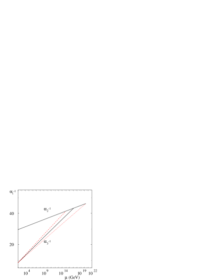
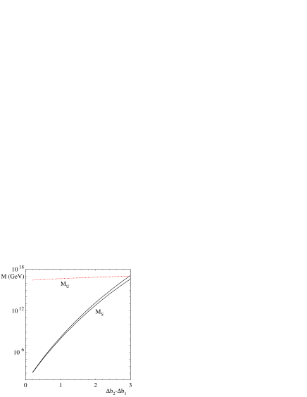
Figure 1: Left: The intersections of the upper solid line with the dashed line, solid line and the dotted line show the one-loop $SU(3)_{C}\times SU(2)_{L}$ gauge coupling unification scale for $(\Delta b_{2}=1,\Delta b_{3}=0)$, $(\Delta b_{2}=1,\Delta b_{3}=1)$, and $(\Delta b_{2}=1,\Delta b_{3}=2)$, respectively. Right: Mass scales $M_{S}$ (solid) and $M_{U}$ (dotted) as functions of $\Delta b_{2}-\Delta b_{1}$ from one-loop RGE running. The upper curves correspond to $M_{V}=200~{}\rm GeV$ and the lower curves $M_{V}=1~{}{\rm TeV}$.

Using the constraints on $\Delta b_{1}$, $\Delta b_{2}$, and $\Delta b_{3}$, we are ready to generate the complete sets of vector-like particles that will ensure canonical gauge coupling unification. Because $\Delta b_{3}=\Delta b_{2}$ and $2/5\leq\Delta b_{2}-\Delta b_{1}\leq 13/5$, there are only finite possibilities for $\Delta b_{2}-\Delta b_{1}$ due to the quantization of $\Delta b_{i}$. We employ the equivalent relations of the one-loop beta function for the particle sets LMN . If we can achieve canonical gauge coupling unification by introducing one set of the vector-like fermions with $\Delta b_{3}=\Delta b_{2}$ and $\Delta b_{2}-\Delta b_{1}=c_{b}$, it also holds for one-loop equivalent sets, defined as those with the same $\Delta b_{3}-\Delta b_{2}$ and $\Delta b_{2}-\Delta b_{1}$ at one loop, because the two-loop effects give only small corrections. The complete independent one-loop beta function equivalent relations for the particle sets are LMN

$$EQV1:XQ+XU+XE\sim 0~{},~{}~{}{\rm or}~{}~{}{\overline{XQ}}+{\overline{XU}}+{\overline{XE}}\sim 0\,;$$ (15)

$$EQV2:XD+XL\sim 0~{},~{}~{}{\rm or}~{}~{}{\overline{XD}}+{\overline{XL}}\sim 0\,;$$ (16)

$$EQV3:XW+XG+XY+{\overline{XY}}\sim 0\,;$$ (17)

$$EQV4:XQ+XT+XS\sim 0~{},~{}~{}{\rm or}~{}~{}{\overline{XQ}}+{\overline{XT}}+{\overline{XS}}\sim 0\,;$$ (18)

$$EQV5:2(XD+{\overline{XD}})+XE+{\overline{XE}}+XW\sim 0\,;$$ (19)

$$EQV6:XL+{\overline{XL}}+2(XE+{\overline{XE}})+XW+XG\sim 0\,;$$ (20)

$$EQV7:XD+XE\sim XU~{},~{}~{}{\rm or}~{}~{}{\overline{XD}}+{\overline{XE}}\sim{\overline{XU}}\,;$$ (21)

$$EQV8:3(XE+{\overline{XE}})+2XW\sim XT+{\overline{XT}}\,;$$ (22)

$$EQV9:XU+XE\sim 2XD+XY~{},~{}~{}{\rm or}~{}~{}{\overline{XU}}+{\overline{XE}}\sim 2{\overline{XD}}+{\overline{XY}}\,.~{}\,$$ (23)

where $0$ means the zero particle set. Equivalent relations (15) – (18) correspond respectively to 10, 5, 24, and 15-plets of $SU(5)$.

The conditions $\Delta b_{2}=\Delta b_{3}$ and $2/5\leq\Delta b_{2}-\Delta b_{3}\leq 13/5$ for canonical gauge coupling unification are satisfied by the simple sets

$$Z1:XW+2(XD+{\overline{XD}})\,,~{}~{}\Delta b=({4\over 5},2,2)\sim(0,{6\over 5},{6\over 5})\,;$$ (24)

$$Z2:XW+3(XD+{\overline{XD}})+(XL+{\overline{XL}})\,,~{}~{}\Delta b=({9\over 5},3,3)\sim(0,{6\over 5},{6\over 5})\,;$$ (25)

$$Z3:XQ+{\overline{XQ}}+XU+{\overline{XU}}\,,~{}~{}\Delta b=({9\over 5},3,3)\sim(0,{6\over 5},{6\over 5})\,;$$ (26)

$$Z4:XQ+{\overline{XQ}}+XD+{\overline{XD}}+XE+{\overline{XE}}\,,~{}~{}\Delta b=({9\over 5},3,3)\sim(0,{6\over 5},{6\over 5})\,;$$ (27)

$$Z5:XG+3(XL+{\overline{XL}})\,,~{}~{}\Delta b=({9\over 5},3,3)\sim(0,{6\over 5},{6\over 5})\,;$$ (28)

$$Z6:XG+XW+XL+{\overline{XL}}+XE+{\overline{XE}}\,,~{}~{}\Delta b=({9\over 5},3,3)\sim(0,{6\over 5},{6\over 5})\,;$$ (29)

$$Z7:XG+XW+XD+{\overline{XD}}+2(XL+{\overline{XL}})+XE+{\overline{XE}}\,,$$

$$~{}~{}~{}~{}~{}~{}~{}~{}~{}~{}~{}~{}\Delta b=({14\over 5},4,4)\sim(0,{6\over 5},{6\over 5})\,;$$ (30)

$$Z8:XQ+{\overline{XQ}}+XD+{\overline{XD}}\,,~{}~{}\Delta b=({3\over 5},3,3)\sim(0,{12\over 5},{12\over 5})\,;$$ (31)

$$Z9:XG+XW+XL+{\overline{XL}}\,,~{}~{}\Delta b=({3\over 5},3,3)\sim(0,{12\over 5},{12\over 5})\,;$$ (32)

$$Z10:XT+{\overline{XT}}+XW+2XG\,,~{}~{}\Delta b=({18\over 5},6,6)\sim(0,{12\over 5},{12\over 5})\,,$$ (33)

all of which either have $\Delta b_{2}-\Delta b_{1}=6/5$ (sets $Zi$, $i=1,\dots,9$) or $\Delta b_{2}-\Delta b_{1}=12/5$ (sets $Z8$, $Z9$, $Z10$). The sets $Zi$ ($i=2,...,7$) may be generated from $Z_{1}$, and $Z9$ and $Z10$ from $Z8$ by using one-loop beta function equivalent relations:

Equiv. sets	Equiv. relations	Equiv. sets	Equiv. relations
$Z2\sim Z1$	2	$Z3\sim Z1$	1, 5
$Z4\sim Z3$	7	$Z5\sim Z1$	2, 5, 6
$Z6\sim Z1$	5, 6	$Z7\sim Z6$	2
$Z9\sim Z8$	1, 6, 7	$Z10\sim Z8$	5, 6, 8

Table 1: Equivalent sets and the equivalent relations involved.

With two-loop RGE running for the gauge couplings and one-loop running for the Yukawa and Higgs quartic coupling, we show the supersymmetry breaking scales, the gauge coupling unification scales and the corresponding Higgs mass ranges for $M_{V}=200~{}\rm GeV$ and 1 TeV in Table 2. The Higgs boson mass ranges correspond to the variation of $\tan\beta$ between 1.5 and 50, with smaller $\tan\beta$ giving a smaller Higgs boson mass, and $\alpha_{s}$ and $m_{t}$ with their $1\sigma$ ranges. For the same $\Delta b_{2}-\Delta b_{1}$, the actual values of $\Delta b_{1}$ and $\Delta b_{2}$, as well as the different two-loop beta functions due to the different additional particle contents can affect RGE running, and hence these mass scales and Higgs boson masses. This is evident in comparing the $Z1$, $Z3$ and $Z5$ sets. The $Z1$ set has different $\Delta b_{1}$ from $Z3$ and $Z5$, while $Z3$ and $Z5$ differ in the two-loop beta functions due to the different extra particles involved. For $Z1$ through $Z9$ the Higgs mass ranges are from about 119 GeV to 143 GeV for $M_{V}=200~{}\rm GeV$ and from about 122 GeV to 145 GeV for $M_{V}=1~{}{\rm TeV}$. The Higgs mass ranges are from 103 GeV to 143 GeV and from 113 GeV to 145 GeV in the model with the $Z10$ set for $M_{V}=200~{}\rm GeV$ and $M_{V}=1~{}{\rm TeV}$, respectively. The Higgs mass ranges are larger (i.e., a lighter Higgs is allowed) in the model with the $Z10$ set than the other models because the values of $\Delta b_{1}$ and $\Delta b_{2}$ are larger. In general, for the models with $\Delta b_{2}-\Delta b_{1}=6/5$, the supersymmetry breaking scale is around $10^{10}~{}\rm GeV$. For those with $\Delta b_{2}-\Delta b_{1}=12/5$, the supersymmetry breaking scale is about $10^{15}~{}\rm GeV$, which can be considered as the GUT scale up to uncertainties from the threshold corrections at the scales $M_{V}$, $M_{S}$, and $M_{U}$. For a particular model with the $Zi$ set, the SM gauge couplings, the Higgs quartic coupling at the supersymmetry breaking scale, as well as the physical Higgs mass will decrease if we increase $M_{V}$.

		$M_{V}=200~{}\rm GeV$			$M_{V}=1000~{}\rm GeV$
$Z$	$\Delta b_{2}-\Delta b_{1}$	$M_{S}$	$M_{U}$	$m_{h}$	$M_{S}$	$M_{U}$	$m_{h}$
$Z1$	6/5	$2.9\times 10^{10}$	$3.6\times 10^{16}$	123 - 144	$1.8\times 10^{10}$	$3.3\times 10^{16}$	125 - 145
$Z2$	6/5	$2.5\times 10^{10}$	$4.4\times 10^{16}$	121 - 143	$1.5\times 10^{10}$	$4.0\times 10^{16}$	124 - 145
$Z3$	6/5	$4.0\times 10^{10}$	$4.0\times 10^{16}$	121 - 143	$2.3\times 10^{10}$	$3.7\times 10^{16}$	124 - 145
$Z4$	6/5	$5.1\times 10^{10}$	$4.0\times 10^{17}$	121 - 143	$2.9\times 10^{10}$	$3.7\times 10^{16}$	124 - 145
$Z5$	6/5	$6.6\times 10^{10}$	$8.1\times 10^{16}$	121 - 143	$4.5\times 10^{10}$	$7.1\times 10^{16}$	123 - 145
$Z6$	6/5	$1.3\times 10^{10}$	$7.0\times 10^{16}$	121 - 143	$8.2\times 10^{10}$	$6.1\times 10^{16}$	123 - 145
$Z7$	6/5	$9.6\times 10^{10}$	$9.8\times 10^{16}$	119 - 143	$6.7\times 10^{10}$	$8.1\times 10^{16}$	122 - 145
$Z8$	12/5	$8.2\times 10^{15}$	$6.2\times 10^{16}$	119 - 143	$3.0\times 10^{15}$	$5.6\times 10^{16}$	123 - 145
$Z9$	12/5	$3.9\times 10^{15}$	$9.6\times 10^{16}$	119 - 143	$1.6\times 10^{15}$	$8.3\times 10^{16}$	123 - 145
$Z10$	12/5	$3.0\times 10^{15}$	$3.1\times 10^{17}$	103 - 143	$1.4\times 10^{15}$	$2.1\times 10^{17}$	113 - 145

Table 2: The supersymmetry breaking scales, the gauge coupling unification scales, and the corresponding Higgs mass ranges for $M_{V}=200~{}\rm GeV$ and $1000~{}\rm GeV$ in the models with $Zi$ sets of vector-like particles. All masses are in GeV.

As an example, we show the two-loop RGE running for the SM gauge couplings in the model with the $Z3$ set in Fig. 2.

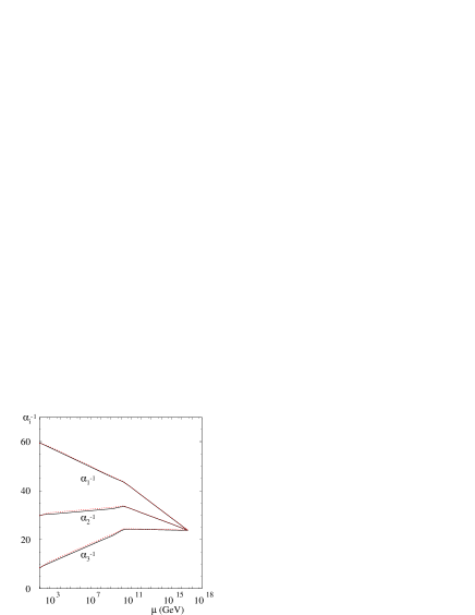
Figure 2: Two-loop gauge coupling unification in the model with the $Z3$ set of vector-like particles. The solid curves are for $M_{V}=200~{}\rm GeV$, while the nearly overlapping dotted curves are for $M_{V}=1~{}{\rm TeV}$.

IV Models with Non-Standard Vector-like Particles

In string model building, we may have vector-like particles which are charged under $SU(3)_{C}\times SU(2)_{L}$ and neutral under $U(1)_{Y}$ Dienes:1996du ; Blumenhagen:2005mu . Often, such particles also carry hidden sector charges. Thus, we introduce such non-standard vector-like particles in this Section. Their quantum numbers under $SU(3)_{C}\times SU(2)_{L}\times U(1)_{Y}$ and their contributions to one-loop beta functions as complete supermultiplets are

$$XQ0+{\overline{XQ0}}={\mathbf{(3,2,0)+({\bar{3}},2,0)}}\,,\quad\Delta b=(0,3,2)\,;$$ (34)

$$XD0+{\overline{XD0}}={\mathbf{({\bar{3}},1,0)+({3},1,0)}}\,,\quad\Delta b=(0,0,1)\,;$$ (35)

$$XL0+{\overline{XL0}}={\mathbf{(1,2,0)+({1},2,0)}}\,,\quad\Delta b=(0,1,0)\,;$$ (36)

$$XS0+{\overline{XS0}}={\mathbf{(6,1,0)+({\bar{6}},1,0)}}\,,\quad\Delta b=(0,0,5)~{}.~{}\,$$ (37)

We do not consider $XU0+\overline{XU0}$, $XT0$ or $XY0+\overline{XY0}$ because they are equivalent to $XD0+\overline{XD0}$, $XW$, and $XQ0+\overline{XQ0}$, respectively.

Note that the states in (34) and (36) have half-integer electric charge, and that the lightest such particles would be stable. Due to the stringent experimental limits on the natural abundances of such particles and their bound states Lee:2002sa , they would have to be much more massive than the reheating temperature after a period of inflation Kudo:2001ie . Thus, for them to exist at the TeV scale the reheating temperature would have to be extremely low Gogoladze:2006si .

The additional independent one-loop beta function equivalent relations for the standard and non-standard particle sets are

$$NEQV1:2XD0+3XL0\sim XQ0~{},~{}~{}{\rm or}~{}~{}2{\overline{XD0}}+3{\overline{XL0}}\sim{\overline{XQ0}}\,;$$ (38)

$$NEQV2:5XD0\sim XS0~{},~{}~{}{\rm or}~{}~{}5{\overline{XD0}}\sim{\overline{XS0}}\,;$$ (39)

$$NEQV3:2XD+XE+2XL0\sim 0~{},~{}~{}{\rm or}~{}~{}2{\overline{XD}}+{\overline{XE}}+2{\overline{XL0}}\sim 0\,;$$ (40)

$$NEQV4:5XE+6XD0+6XL0\sim 0~{},~{}~{}{\rm or}~{}~{}5{\overline{XE}}+6{\overline{XD0}}+6{\overline{XL0}}\sim 0\,.~{}\,$$ (41)

We consider the following simple sets of standard and non-standard vector-like particles

$$NZ1:XD0+{\overline{XD0}}+XL+{\overline{XL}}\,,~{}~{}\Delta b=({3\over 5},1,1)\sim(0,{2\over 5},{2\over 5})\,;$$ (42)

$$NZ2:4(XD0+{\overline{XD0}})+XT+{\overline{XT}}\,,~{}~{}\Delta b=({18\over 5},4,4)\sim(0,{2\over 5},{2\over 5})\,;$$ (43)

$$NZ3:XL0+{\overline{XL0}}+XD+{\overline{XD}}\,,~{}~{}\Delta b=({2\over 5},1,1)\sim(0,{3\over 5},{3\over 5})\,;$$ (44)

$$NZ4:2(XD0+{\overline{XD0}})+XW+XE+{\overline{XE}}\,,~{}~{}\Delta b=({6\over 5},2,2)\sim(0,{4\over 5},{4\over 5})\,;$$ (45)

$$NZ5:XD0+{\overline{XD0}}+XL0+{\overline{XL0}}\,,~{}~{}~{}\Delta b=(0,1,1)\,;$$ (46)

$$NZ6:XQ0+{\overline{XQ0}}+XU+{\overline{XU}}\,,~{}~{}\Delta b=({8\over 5},3,3)\sim(0,{7\over 5},{7\over 5})\,;$$ (47)

$$NZ7:XQ0+{\overline{XQ0}}+XD+{\overline{XD}}+XE+{\overline{XE}}\,,~{}~{}\Delta b=({8\over 5},3,3)\sim(0,{7\over 5},{7\over 5})\,;$$ (48)

$$NZ8:XD0+{\overline{XD0}}+XD+{\overline{XD}}+XW\,,~{}~{}\Delta b=({2\over 5},2,2)\sim(0,{8\over 5},{8\over 5})\,;$$ (49)

$$NZ9:XL0+{\overline{XL0}}+XG+2(XL+{\overline{XL}})\,,~{}~{}\Delta b=({6\over 5},3,3)\sim(0,{9\over 5},{9\over 5})\,;$$ (50)

$$NZ10:2(XD0+{\overline{XD0}})+XW\,,~{}~{}\Delta b=(0,2,2)\,;$$ (51)

$$NZ11:XS0+5(XL+{\overline{XL}})\,,~{}~{}\Delta b=(3,5,5)\sim(0,2,2)\,;$$ (52)

$$NZ12:XD0+{\overline{XD0}}+XL0+{\overline{XL0}}+XQ+{\overline{XQ}}+XU+{\overline{XU}}\,,$$

$$\quad\quad\quad~{}~{}\Delta b=({9\over 5},4,4)\sim(0,{11\over 5},{11\over 5})\,;$$ (53)

$$NZ13:2(XL0+{\overline{XL0}})+XG+XL+{\overline{XL}}\,,~{}~{}\Delta b=({3\over 5},3,3)\sim(0,{12\over 5},{12\over 5})\,;$$ (54)

$$NZ14:2(XL0+{\overline{XL0}})+XT+{\overline{XT}}+2XG\,,~{}~{}\Delta b=({18\over 5},6,6)\sim(0,{12\over 5},{12\over 5})\,;$$ (55)

$$NZ15:XQ0+{\overline{XQ0}}+XD+{\overline{XD}}\,,~{}~{}\Delta b=({2\over 5},3,3)\sim(0,{13\over 5},{13\over 5})\,.$$ (56)

		$M_{V}=200~{}\rm GeV$			$M_{V}=1000~{}\rm GeV$
$NZ$	$\Delta b_{2}-\Delta b_{1}$	$M_{S}$	$M_{U}$	$m_{h}$	$M_{S}$	$M_{U}$	$m_{h}$
$NZ1$	2/5	$5.7\times 10^{5}$	$2.4\times 10^{16}$	114 - 139	$4.8\times 10^{5}$	$2.3\times 10^{16}$	114 - 139
$NZ2$	2/5	$1.8\times 10^{6}$	$2.9\times 10^{16}$	114 - 140	$1.6\times 10^{6}$	$6.4\times 10^{16}$	107 - 139
$NZ3$	3/5	$9.0\times 10^{6}$	$2.6\times 10^{16}$	119 - 142	$1.4\times 10^{6}$	$3.6\times 10^{16}$	115 - 144
$NZ4$	4/5	$2.6\times 10^{8}$	$3.0\times 10^{16}$	121 - 143	$1.8\times 10^{8}$	$2.8\times 10^{16}$	122 - 144
$NZ5$	1	$1.9\times 10^{9}$	$3.1\times 10^{16}$	124 - 144	$1.2\times 10^{9}$	$3.0\times 10^{16}$	125 - 145
$NZ6$	7/5	$3.9\times 10^{11}$	$4.3\times 10^{16}$	121 - 144	$2.1\times 10^{11}$	$4.0\times 10^{16}$	124 - 145
$NZ7$	7/5	$4.9\times 10^{11}$	$4.3\times 10^{16}$	121 - 144	$2.5\times 10^{11}$	$4.0\times 10^{16}$	124 - 145
$NZ8$	8/5	$2.7\times 10^{12}$	$4.2\times 10^{16}$	124 - 144	$1.3\times 10^{11}$	$3.9\times 10^{16}$	126 - 146
$NZ9$	9/5	$7.3\times 10^{12}$	$9.1\times 10^{16}$	121 - 143	$3.8\times 10^{12}$	$7.9\times 10^{16}$	124 - 145
$NZ10$	2	$1.5\times 10^{14}$	$4.8\times 10^{16}$	124 - 144	$6.5\times 10^{13}$	$4.5\times 10^{16}$	126 - 146
$NZ11$	2	$2.2\times 10^{13}$	$3.1\times 10^{17}$	113 - 142	$1.2\times 10^{13}$	$2.3\times 10^{17}$	119 - 145
$NZ12$	11/5	$1.2\times 10^{15}$	$7.4\times 10^{16}$	116 - 143	$4.7\times 10^{14}$	$6.5\times 10^{16}$	121 - 145
$NZ13$	12/5	$2.9\times 10^{15}$	$1.1\times 10^{17}$	120 - 143	$1.2\times 10^{15}$	$9.1\times 10^{16}$	123 - 145
$NZ14$	12/5	$2.0\times 10^{15}$	$3.6\times 10^{17}$	104 - 143	$9.8\times 10^{14}$	$2.4\times 10^{17}$	113 - 145
$NZ15$	13/5	$4.7\times 10^{16}$	$6.6\times 10^{16}$	118 - 143	$1.6\times 10^{16}$	$6.0\times 10^{16}$	123 - 145

Table 3: Same as Table 2, only for the $NZi$ sets.

With the non-standard vector-like particles, $\Delta b_{2}-\Delta b_{1}$ can be $n/5$, where $n=2,3,...,13$. The sets with $\Delta b_{3}=\Delta b_{2}$ and $\Delta b_{2}-\Delta b_{1}=6/5$ are given in the previous Section. Simple estimates of the supersymmetry breaking scales and the unification scales from one-loop RGE running are already presented in the right plot of Fig. 1. With two-loop RGE running for the SM gauge couplings and one-loop running for the Yukawa couplings and Higgs quartic coupling included, we present the more reliable supersymmetry breaking scales, gauge coupling unification scales and the corresponding Higgs boson mass ranges in Table 3. The supersymmetry breaking scales can be from $10^{5}~{}\rm GeV$ to the GUT scale if we include the uncertainties from threshold corrections at $M_{V}$, $M_{S}$ and $M_{U}$. In general, the supersymmetry breaking scale will be higher for the models with larger $\Delta b_{2}-\Delta b_{1}$.

We show the two-loop RGE running of the SM gauge couplings in the model with the $NZ1$ set in Fig. 3. Because of the smaller $\Delta b_{2}-\Delta b_{1}$ value, the supersymmetry breaking scale is lower compared to Fig. 2.

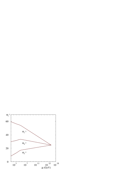
Figure 3: Same as Fig. 2, only for the $NZ1$ set.

V Comments on the Phenomenological Consequences

We now address the problem of how vector-like particles have masses at the electroweak scale. Since mass terms of vector-like particles are invariant under the Standard Model gauge group, we are allowed to write terms like $\overline{XQ}\,XQ$ in the Lagrangian, and the natural scale of this mass might be the unification scale. This would then lead to a new fine tuning problem. A natural mechanism to forbid such mass terms is to embed the particles in a larger symmetry group such that the only mass terms allowed are through Yukawa couplings with a singlet field $S$, for example $S\,\overline{XQ}\,XQ$, with $S$ having a VEV at the electroweak scale. This is the mechanism of mass generation of vector-like down-type quarks based on the group $E_{6}$ which could arise from heterotic string compactification. The question of why vector-like particles do not occur in complete GUT multiplets can be understood by breaking the GUT symmetry via Wilson lines Braun:2005ux or orbifold projections Orbifold . Another consequence of the singlet field $S$ is that we can obtain a strong first order electroweak phase transition with the presence of the trilinear interaction $SH^{\dagger}H$ in the Higgs potential, similar to the next to the Minimal Supersymmetric Standard Model Pietroni ; DFMHS and the supersymmetric $U(1)^{\prime}$ model Kang:2004pp .

The vector-like fermions can yield rich low energy phenomenology. Models with $XD$ and $\overline{XD}$ have received a lot of attention because they naturally occur in heterotic string inspired $E_{6}$ models Barger:1985nq . It is interesting to note that transformation under the Standard Model gauge group does not uniquely specify all the properties of such vector-like particles. For example, the superpotential of $XD$ and $\overline{XD}$ has to be defined before a complete description can be given. Three possibilities depending on lepton and baryon number assignments are (a) down type quark, (b) leptoquark, and (c) diquark. For a review of the production and decays of these particles see Ref. Hewett:1988xc ; KLN . They may also be quasi-stable decaying only by higher-dimensional operators Fairbairn:2006gg with cosmological and collider implications KLN ; Fairbairn:2006gg . For the models with $XU$ and ${\overline{XU}}$, there are new effects in top and charm quark (e.g., $D$ meson) physics, while for the models with $XD$ and ${\overline{XD}}$, we have new effects in $B$ physics Morrissey:2003sc ; Barger:1995dd ; Deshpande:2003nx . Also, models with $XQ$, ${\overline{XQ}}$, $XD$ and ${\overline{XD}}$ can explain the bottom quark forward-backward asymmetry ($A_{FB}^{b}$) Choudhury:2001hs . Neutrino masses and mixings can be generated if there exist $XW$ and $XL$/$\overline{XL}$, or two $XW$, or two $XL$/$\overline{XL}$. The neutral component of $XW$ or $XL/{\overline{XL}}$ can be a cold dark matter candidate if there exists a discrete symmetry and their masses are around the TeV scale REST . The models with $XW$, $XL$, and ${\overline{XL}}$, may not only explain the dark matter but also generate the baryon asymmetry via electroweak baryogenesis Carena:2004ha . Similar to split supersymmetry, the supersymmetry breaking scale may not be higher than $10^{12}~{}\rm GeV$ in the models with $XG$ and the standard vector-like quarks because $XG$ cannot decay fast enough via Yukawa couplings in the superpotential to satisfy cosmological constraints Arvanitaki:2005fa . For models with $XG$ but no other standard vector-like quarks, the cosmological constraint on $XG$ and the phenomenological consequences deserve detailed study because $XG$ can be stable at least in some orbifold models. Similarly, whether the non-standard vector-like particles can decay, and the cosmological constraints on the non-standard vector-like particles and their phenomenological consequences deserve further detailed study.

Let us focus on the experimentally viable models which have standard vector-like particles. Suppose that the axion is the cold dark matter candidate, and we introduce two or three right-handed neutrinos to explain the neutrino masses and mixings and the baryon asymmetry. The simple models with $10^{10}$ GeV-scale supersymmetry breaking are those with $Z1$ and $Z3$ sets, and the simplest with $10^{15}$ GeV-scale supersymmetry breaking is the one with the $Z8$ set. If that axion does not contribute to the dominant cold dark matter density, and the neutrino masses and mixings are generated due to the $R-$parity violating terms Grossman:2003gq , the model with the $Z2$ set is the simplest which has a dark matter candidate and can explain the baryon asymmetry.

The phenomenological consequences of our models, for example, new effects in the meson physics, CP violation, and the collider signatures at the LHC will be presented in detail elsewhere.

VI Discussions and Conclusions

We studied the canonical gauge coupling unification in the extensions of the SM with universal high-scale supersymmetry breaking by introducing additional SM vector-like fermions. To avoid the dimension-6 proton decay problem and quantum gravity effects, we require that the gauge coupling unification scale is from $5\times 10^{15}$ GeV to the Planck scale. We assume that the supersymmetry breaking scale is below the unification scale, and that the universal masses of the vector-like fermions are from 200 GeV to 1 TeV. In order to have the canonical gauge coupling unification and to satisfy these requirements and assumptions, we showed that $\Delta b_{2}=\Delta b_{3}$ and $2/5\leq\Delta b_{2}-\Delta b_{1}\leq 13/5$ for the extra vector-like particles. To systematically construct the models with canonical gauge coupling unification, we used the technique of the one-loop beta function equivalent relations for the particle sets. We discussed two kinds of models. The first kind of models have standard vector-like particles while the second kind of models have standard and non-standard ones. In the models with simple sets of extra vector-like fermions whose universal masses are $200$ GeV and $1~{}{\rm TeV}$, we presented the supersymmetry breaking scales, gauge coupling unification scales, and the corresponding Higgs mass ranges. In the first kind of models, $\Delta b_{2}-\Delta b_{1}$ can only be equal to $6/5$ and $12/5$, and then the corresponding supersymmetry breaking scale can only be around $10^{10}$ GeV and $10^{15}$ GeV, respectively. In the second kind, $\Delta b_{2}-\Delta b_{1}$ can be $n/5$, in which $n=2,3,...,13$, so the supersymmetry breaking scale can be from $10^{5}$ GeV to $10^{16}$ GeV. Because the universal masses for the vector-like fermions are within the reach of the LHC, these models can definitely be tested at the LHC.

We briefly commented on some phenomenological consequences of these models, which deserve further detailed study.

Appendix A Renormalization Group Equations

In this Appendix, we give the renormalization group equations in the SM and MSSM. The general formulae for the renormalization group equations in the SM are given in Refs. mac ; Cvetic:1998uw , and those for the supersymmetric models in Refs. Barger:1992ac ; Barger:1993gh ; Martin:1993zk .

First, we summarize the renormalization group equations in the SM. The two-loop equations for the gauge couplings are

$$(4\pi)^{2}\frac{d}{dt}~{}g_{i}=g_{i}^{3}b_{i} + \frac{g_{i}^{3}}{(4\pi)^{2}}\left[\sum_{j=1}^{3}B_{ij}g_{j}^{2}-\sum_{\alpha=u,d,e}d_{i}^{\alpha}{\rm Tr}\left(h^{\alpha\dagger}h^{\alpha}\right)\right]~{},~{}\,$$ (57)

where $t=\ln\mu$ and $\mu$ is the renormalization scale. $g_{1}$, $g_{2}$ and $g_{3}$ are the gauge couplings for $U(1)_{Y}$, $SU(2)_{L}$ and $SU(3)_{C}$, respectively, where we use the $SU(5)$ normalization $g_{1}^{2}\equiv(5/3)g_{Y}^{2}$. The beta-function coefficients are

$$b=\left(\frac{41}{10},-\frac{19}{6},-7\right)~{},~{}B=\pmatrix{\frac{199}{50}&\frac{27}{10}&\frac{44}{5}\cr\frac{9}{10}&\frac{35}{6}&12\cr\frac{11}{10}&\frac{9}{2}&-26}~{},~{}$$ (58)

$$d^{u}=\left(\frac{17}{10},\frac{3}{2},2\right)~{},~{}d^{d}=\left(\frac{1}{2},\frac{3}{2},2\right)~{},~{}d^{e}=\left(\frac{3}{2},\frac{1}{2},0\right)~{}.~{}\,$$ (59)

Since the contributions in Eq. (57) from the Yukawa couplings arise from the two-loop diagrams, we only need Yukawa coupling evolution at one-loop order. The one-loop renormalization group equations for the Yukawa couplings are

$$(4\pi)^{2}\frac{d}{dt}~{}h^{u} = h^{u}\left(-\sum_{i=1}^{3}c_{i}^{u}g_{i}^{2}+\frac{3}{2}h^{u\dagger}h^{u}-\frac{3}{2}h^{d\dagger}h^{d}+\Delta_{2}\right)~{},~{}$$ (60)

$$(4\pi)^{2}\frac{d}{dt}~{}h^{d} = h^{d}\left(-\sum_{i=1}^{3}c_{i}^{d}g_{i}^{2}-\frac{3}{2}h^{u\dagger}h^{u}+\frac{3}{2}h^{d\dagger}h^{d}+\Delta_{2}\right)~{},~{}$$ (61)

$$(4\pi)^{2}\frac{d}{dt}~{}h^{e} = h^{e}\left(-\sum_{i=1}^{3}c_{i}^{e}g_{i}^{2}+\frac{3}{2}h^{e\dagger}h^{e}+\Delta_{2}\right)~{},~{}\,$$ (62)

where $h^{u}$, $h^{d}$ and $h^{e}$ are the Yukawa couplings for the up-type quark, down-type quark, and lepton, respectively. Also, $c^{u}$, $c^{d}$, and $c^{e}$ are given by

$$c^{u}=\left(\frac{17}{20},\frac{9}{4},8\right)~{},~{}c^{d}=\left(\frac{1}{4},\frac{9}{4},8\right)~{},~{}c^{e}=\left(\frac{9}{4},\frac{9}{4},0\right)~{},~{}$$ (63)

and

$$\Delta_{2} = {\rm Tr}(3h^{u\dagger}h^{u}+3h^{d\dagger}h^{d}+h^{e\dagger}h^{e})~{}.~{}$$ (64)

The one-loop renormalization group equation for the Higgs quartic coupling is

$$(4\pi)^{2}\frac{d}{dt}~{}\lambda = 12\lambda^{2}-\left({9\over 5}g_{1}^{2}+9g_{2}^{2}\right)\lambda+{9\over 4}\left({3\over{25}}g_{1}^{4}+{2\over 5}g_{1}^{2}g_{2}^{2}+g_{2}^{4}\right)+4\Delta_{2}\lambda-4\Delta_{4}~{},~{}\,$$ (65)

where

$$\Delta_{4} = {\rm Tr}\left[3(h^{u\dagger}h^{u})^{2}+3(h^{d\dagger}h^{d})^{2}+(h^{e\dagger}h^{e})^{2}\right]~{}.~{}$$ (66)

Next, we summarize the renormalization group equations in the MSSM. The two-loop renormalization group equations for the gauge couplings are

$$(4\pi)^{2}\frac{d}{dt}~{}g_{i} = g_{i}^{3}b_{i}+\frac{g_{i}^{3}}{(4\pi)^{2}}\left[~{}\sum_{j=1}^{3}B_{ij}g_{j}^{2}-\sum_{\alpha=u,d,e}d_{i}^{\alpha}{\rm Tr}\left(y^{\alpha\dagger}y^{\alpha}\right)\right]~{},~{}\,$$ (67)

where the beta-function coefficients are

$$b=\left(\frac{33}{5},1,-3\right)~{},~{}~{}~{}B=\pmatrix{\frac{199}{25}&\frac{27}{5}&\frac{88}{5}\cr\frac{9}{5}&25&24\cr\frac{11}{5}&9&14}~{},~{}$$ (68)

$$d^{u}=\left(\frac{26}{5},6,4\right)~{},~{}d^{d}=\left(\frac{14}{5},6,4\right)~{},~{}d^{e}=\left(\frac{18}{5},2,0\right)~{}.~{}$$ (69)

The one-loop renormalization group equations for Yukawa couplings are

$$(4\pi)^{2}\frac{d}{dt}~{}y^{u} = y^{u}\left[3y^{u\dagger}y^{u}+y^{d\dagger}y^{d}+3{\rm Tr}(y^{u\dagger}y^{u})-\sum_{i=1}^{3}c_{i}^{u}g_{i}^{2}\right]~{},~{}$$ (71)

$$(4\pi)^{2}\frac{d}{dt}~{}y^{d} = y^{d}\left[y^{u\dagger}y^{u}+3y^{d\dagger}y^{d}+{\rm Tr}(3y^{d\dagger}y^{d}+y^{e\dagger}y^{e})-\sum_{i=1}^{3}c_{i}^{d}g_{i}^{2}\right]~{},~{}$$ (72)

$$(4\pi)^{2}\frac{d}{dt}~{}y^{e} = y^{e}\left[3y^{e\dagger}y^{e}+{\rm Tr}(3y^{d\dagger}y^{d}+y^{e\dagger}y^{e})-\sum_{i=1}^{3}c_{i}^{e}g_{i}^{2}\right]~{},~{}\,$$ (73)

where $y^{u}$, $y^{d}$ and $y^{e}$ are the Yukawa couplings for the up-type quark, down-type quark, and lepton, respectively. $c^{u}$, $c^{d}$, and $c^{e}$ are given by

$$c^{u}=\left(\frac{13}{15},3,\frac{16}{3}\right)~{},~{}c^{d}=\left(\frac{7}{15},3,\frac{16}{3}\right)~{},~{}c^{e}=\left(\frac{9}{5},3,0\right)~{}.~{}\,$$ (74)

Appendix B Two-Loop Beta Functions for the Vector-Like Particles

In this Appendix, we present two-loop beta functions contributions to the SM gauge couplings from the vector-like particles which are introduced in Sections III and IV. The general formulae are also given in Refs. mac ; Cvetic:1998uw ; Barger:1992ac ; Barger:1993gh ; Martin:1993zk .

The two-loop beta functions ($\Delta B_{ij}$) from the extra particles in the non-supersymmetric models are

$$\Delta B^{XQ+{\overline{XQ}}}=\pmatrix{\frac{1}{150}&\frac{3}{10}&\frac{8}{15}\cr\frac{1}{10}&\frac{49}{2}&8\cr\frac{1}{15}&3&\frac{76}{3}}~{},~{}\Delta B^{XU+{\overline{XU}}}=\pmatrix{\frac{64}{75}&0&\frac{64}{15}\cr 0&0&0\cr\frac{8}{15}&0&\frac{38}{3}}~{},~{}\,$$ (75)

$$\Delta B^{XD+{\overline{XD}}}=\pmatrix{\frac{4}{75}&0&\frac{16}{15}\cr 0&0&0\cr\frac{2}{15}&0&\frac{38}{3}}~{},~{}\Delta B^{XL+{\overline{XL}}}=\pmatrix{\frac{9}{50}&\frac{9}{10}&0\cr\frac{3}{10}&\frac{49}{6}&0\cr 0&0&0}~{},~{}\,$$ (76)

$$\Delta B^{XE+{\overline{XE}}}=\pmatrix{\frac{36}{25}&0&0\cr 0&0&0\cr 0&0&0}~{},~{}\Delta B^{XG}=\pmatrix{0&0&0\cr 0&0&0\cr 0&0&48}~{},~{}\,$$ (77)

$$\Delta B^{XW}=\pmatrix{0&0&0\cr 0&\frac{64}{3}&0\cr 0&0&0}~{},~{}\Delta B^{XT+{\overline{XT}}}=\pmatrix{\frac{108}{25}&\frac{72}{5}&0\cr\frac{24}{5}&\frac{128}{3}&0\cr 0&0&0}~{},~{}\,$$ (78)

$$\Delta B^{XS+{\overline{XS}}}=\pmatrix{\frac{128}{75}&0&\frac{64}{3}\cr 0&0&0\cr\frac{8}{3}&0&\frac{250}{3}}~{},~{}\Delta B^{XY+{\overline{XY}}}=\pmatrix{\frac{25}{6}&\frac{15}{2}&\frac{40}{3}\cr\frac{5}{2}&\frac{49}{2}&8\cr\frac{5}{3}&3&\frac{76}{3}}~{},~{}\,$$ (79)

$$\Delta B^{XQ0+{\overline{XQ0}}}=\pmatrix{0&0&0\cr 0&\frac{49}{2}&8\cr 0&3&\frac{76}{3}}~{},~{}\Delta B^{XD0+{\overline{XD0}}}=\pmatrix{0&0&0\cr 0&0&0\cr 0&0&\frac{38}{3}}~{},~{}\,$$ (80)

$$\Delta B^{XL0+{\overline{XL0}}}=\pmatrix{0&0&0\cr 0&\frac{49}{6}&0\cr 0&0&0}~{},~{}\Delta B^{XS+{\overline{XS}}}=\pmatrix{0&0&0\cr 0&0&0\cr 0&0&\frac{250}{3}}~{}.~{}\,$$ (81)

In the supersymmetric models

$$\Delta B^{XQ+{\overline{XQ}}}=\pmatrix{\frac{1}{75}&\frac{3}{5}&\frac{16}{15}\cr\frac{1}{5}&21&16\cr\frac{2}{15}&6&\frac{68}{3}}~{},~{}\Delta B^{XU+{\overline{XU}}}=\pmatrix{\frac{128}{75}&0&\frac{128}{15}\cr 0&0&0\cr\frac{16}{15}&0&\frac{34}{3}}~{},~{}\,$$ (82)

$$\Delta B^{XD+{\overline{XD}}}=\pmatrix{\frac{8}{75}&0&\frac{32}{15}\cr 0&0&0\cr\frac{4}{15}&0&\frac{34}{3}}~{},~{}\Delta B^{XL+{\overline{XL}}}=\pmatrix{\frac{9}{25}&\frac{9}{5}&0\cr\frac{3}{5}&7&0\cr 0&0&0}~{},~{}\,$$ (83)

$$\Delta B^{XE+{\overline{XE}}}=\pmatrix{\frac{72}{25}&0&0\cr 0&0&0\cr 0&0&0}~{},~{}\Delta B^{XG}=\pmatrix{0&0&0\cr 0&0&0\cr 0&0&54}~{},~{}\,$$ (84)

$$\Delta B^{XW}=\pmatrix{0&0&0\cr 0&24&0\cr 0&0&0}~{},~{}\Delta B^{XT+{\overline{XT}}}=\pmatrix{\frac{216}{25}&\frac{144}{5}&0\cr\frac{48}{5}&48&0\cr 0&0&0}~{},~{}\,$$ (85)

$$\Delta B^{XS+{\overline{XS}}}=\pmatrix{\frac{256}{75}&0&\frac{128}{3}\cr 0&0&0\cr\frac{16}{3}&0&\frac{290}{3}}~{},~{}\Delta B^{XY+{\overline{XY}}}=\pmatrix{\frac{25}{3}&15&\frac{80}{3}\cr 5&21&16\cr\frac{10}{3}&6&\frac{68}{3}}~{},~{}\,$$ (86)

$$\Delta B^{XQ0+{\overline{XQ0}}}=\pmatrix{0&0&0\cr 0&21&16\cr 0&6&\frac{68}{3}}~{},~{}\Delta B^{XD0+{\overline{XD0}}}=\pmatrix{0&0&0\cr 0&0&0\cr 0&0&\frac{34}{3}}~{},~{}\,$$ (87)

$$\Delta B^{XL0+{\overline{XL0}}}=\pmatrix{0&0&0\cr 0&7&0\cr 0&0&0}~{},~{}\Delta B^{XS0+{\overline{XS0}}}=\pmatrix{0&0&0\cr 0&0&0\cr 0&0&\frac{290}{3}}~{}.~{}\,$$ (88)

References

• (1) R. Bousso and J. Polchinski, JHEP 0006, 006 (2000); S. B. Giddings, S. Kachru and J. Polchinski, Phys. Rev. D 66, 106006 (2002); S. Kachru, R. Kallosh, A. Linde and S. P. Trivedi, Phys. Rev. D 68, 046005 (2003); L. Susskind, arXiv:hep-th/0302219; F. Denef and M. R. Douglas, JHEP 0405, 072 (2004); JHEP 0503, 061 (2005).
• (2) S. Weinberg, Phys. Rev. Lett.  59 2607 (1987).
• (3) V. Agrawal, S. M. Barr, J. F. Donoghue and D. Seckel, Phys. Rev. Lett.  80, 1822 (1998); Phys. Rev. D 57, 5480 (1998).
• (4) J. F. Donoghue, Phys. Rev. D 69, 106012 (2004) [Erratum-ibid. D 69, 129901 (2004)].
• (5) R. D. Peccei and H. R. Quinn, Phys. Rev. Lett. 38 1440 (1977); Phys. Rev. D16 1791 (1977).
• (6) K. S. Babu, I. Gogoladze and K. Wang, Phys. Lett. B 560, 214 (2003).
• (7) V. Barger, C. W. Chiang, J. Jiang and T. Li, Nucl. Phys. B 705, 71 (2005).
• (8) M. B. Green and J. H. Schwarz, Phys. Lett. B149 117 (1984); Nucl. Phys. B255 93 (1985); M. B. Green, J. H. Schwarz and P. West, Nucl. Phys. B254 327 (1985).
• (9) P. Svrcek and E. Witten, JHEP 0606 (2006) 051 [arXiv:hep-th/0605206].
• (10) A. Giryavets, S. Kachru and P. K. Tripathy, JHEP 0408 002 (2004); L. Susskind, arXiv:hep-th/0405189; M. R. Douglas, arXiv:hep-th/0405279; arXiv:hep-th/0409207; M. Dine, E. Gorbatov and S. Thomas, arXiv:hep-th/0407043; E. Silverstein, arXiv:hep-th/0407202; J. P. Conlon and F. Quevedo, JHEP 0410, 039 (2004); M. Dine, D. O’Neil and Z. Sun, JHEP 0507, 014 (2005).
• (11) N. Arkani-Hamed and S. Dimopoulos, JHEP 0506, 073 (2005).
• (12) P. G. Camara, L. E. Ibanez and A. M. Uranga, Nucl. Phys. B 708, 268 (2005); L. E. Ibáñez, Phys. Rev. D 71, 055005 (2005); A. Font and L. E. Ibanez, JHEP 0503, 040 (2005).
• (13) D. Lüst, S. Reffert and S. Stieberger, Nucl. Phys. B 727, 264 (2005); Nucl. Phys. B 706, 3 (2005).
• (14) H. Georgi and S. L. Glashow, Phys. Rev. Lett.  32, 438 (1974); P. Langacker and M. X. Luo, Phys. Rev. D 44, 817 (1991); J. R. Ellis, S. Kelley and D. V. Nanopoulos, Phys. Lett. B 260, 131 (1991); U. Amaldi, W. de Boer and H. Furstenau, Phys. Lett. B 260, 447 (1991).
• (15) P. H. Frampton and S. L. Glashow, Phys. Lett. B 131, 340 (1983) [Erratum-ibid. B 135, 515 (1984)]. S. Nandi, Phys. Lett. B 142, 375 (1984); H. Murayama and T. Yanagida, Mod. Phys. Lett. A 7, 147 (1992); T. G. Rizzo, Phys. Rev. D 45, 3903 (1992); G. F. Giudice and A. Romanino, Nucl. Phys. B 699, 65 (2004) [Erratum-ibid. B 706, 65 (2005)].
• (16) D. Choudhury, T. M. P. Tait and C. E. M. Wagner, Phys. Rev. D 65, 053002 (2002).
• (17) D. E. Morrissey and C. E. M. Wagner, Phys. Rev. D 69, 053001 (2004).
• (18) A. Kehagias and N. D. Tracas, arXiv:hep-ph/0506144.
• (19) V. Barger, J. Jiang, P. Langacker and T. Li, Phys. Lett. B 624, 233 (2005); Nucl. Phys. B 726, 149 (2005).
• (20) W. M. Yao et al. [Particle Data Group], J. Phys. G 33, 1 (2006).
• (21) M. Cvetic, D. A. Demir, J. R. Espinosa, L. L. Everett and P. Langacker, Phys. Rev. D 56, 2861 (1997) [Erratum-ibid. D 58, 119905 (1998)] [arXiv:hep-ph/9703317].
• (22) T. Li, H. Murayama and S. Nandi, unpublished.
• (23) K. R. Dienes, Phys. Rept.  287, 447 (1997).
• (24) R. Blumenhagen, M. Cvetic, P. Langacker and G. Shiu, Ann. Rev. Nucl. Part. Sci.  55, 71 (2005).
• (25) H. Davoudiasl, R. Kitano, T. Li and H. Murayama, Phys. Lett. B 609, 117 (2005).
• (26) H. Fritzsch and P. Minkowski, Phys. Lett. B 62, 72 (1976); M. Gell-Mann, P. Ramond, and R. Slansky, in Supergravity, ed. F. van Nieuwenhuizen and D. Freedman, (North Holland, Amsterdam, 1979) p. 315; T. Yanagida, Proc. of the Workshop on Unified Theory and the Baryon Number of the Universe, KEK, Japan, 1979; S. Weinberg, Phys. Rev. Lett.  43, 1566 (1979); R. N. Mohapatra and G. Senjanovic, Phys. Rev. Lett. 44, 912 (1980).
• (27) M. Fukugita and T. Yanagida, Phys. Lett. B 174, 45 (1986); P. H. Frampton, S. L. Glashow and T. Yanagida, Phys. Lett. B 548, 119 (2002); V. Barger, D. A. Dicus, H. J. He and T. Li, Phys. Lett. B 583, 173 (2004).
• (28) V. Barger, J. Jiang, P. Langacker and T. Li, arXiv:hep-ph/0612206.
• (29) I. Gogoladze, T. Li and Q. Shafi, arXiv:hep-ph/0602040.
• (30) H. Arason, D. J. Castano, B. Keszthelyi, S. Mikaelian, E. J. Piard, P. Ramond and B. D. Wright, Phys. Rev. D 46, 3945 (1992); H. E. Haber, R. Hempfling and A. H. Hoang, Z. Phys. C 75, 539 (1997).
• (31) [CDF Collaboration], arXiv:hep-ex/0507091.
• (32) E. Brubaker et al. [Tevatron Electroweak Working Group], arXiv:hep-ex/0608032.
• (33) S. Bethke, arXiv:hep-ex/0606035.
• (34) I. T. Lee et al., Phys. Rev. D 66, 012002 (2002) [arXiv:hep-ex/0204003]; M. L. Perl, E. R. Lee and D. Loomba, Mod. Phys. Lett. A 19, 2595 (2004).
• (35) A. Kudo and M. Yamaguchi, Phys. Lett. B 516, 151 (2001) [arXiv:hep-ph/0103272].
• (36) I. Gogoladze, T. Li, V. N. Senoguz and Q. Shafi, Phys. Rev. D 74, 126006 (2006) [arXiv:hep-ph/0608181].
• (37) M. Pietroni, Nucl. Phys. B402, 27 (1993).
• (38) A. T. Davies, C. D. Froggatt and R. G. Moorhouse, Phys. Lett. B 372, 88 (1996); S. J. Huber and M. G. Schmidt, Eur. Phys. J. C10, 473 (1999); Nucl. Phys. B 606, 183 (2001).
• (39) J. Kang, P. Langacker, T. Li and T. Liu, Phys. Rev. Lett.  94, 061801 (2005).
• (40) V. Braun, Y. H. He, B. A. Ovrut and T. Pantev, Phys. Lett. B 618, 252 (2005).
• (41) Y. Kawamura, Prog. Theor. Phys.  103, 613 (2000); G. Altarelli and F. Feruglio, Phys. Lett. B 511, 257 (2001); L. Hall and Y. Nomura, Phys. Rev. D 64, 055003 (2001); A. Hebecker and J. March-Russell, Nucl. Phys. B 613, 3 (2001); T. Li, Phys. Lett. B 520, 377 (2001); Nucl. Phys. B 619, 75 (2001).
• (42) V. D. Barger, N. Deshpande, R. J. N. Phillips and K. Whisnant, Phys. Rev. D 33, 1912 (1986) [Erratum-ibid. D 35, 1741 (1987)].
• (43) J. L. Hewett and T. G. Rizzo, Phys. Rept.  183, 193 (1989).
• (44) J. Kang, P. Langacker, and B. D. Nelson, in preparation.
• (45) M. Fairbairn, A. C. Kraan, D. A. Milstead, T. Sjostrand, P. Skands and T. Sloan, arXiv:hep-ph/0611040.
• (46) V. D. Barger, M. S. Berger and R. J. N. Phillips, Phys. Rev. D 52, 1663 (1995) [arXiv:hep-ph/9503204].
• (47) N. G. Deshpande and D. K. Ghosh, Phys. Lett. B 593, 135 (2004).
• (48) R. Essig and S. Thomas, in preparation.
• (49) M. Carena, A. Megevand, M. Quiros and C. E. M. Wagner, Nucl. Phys. B 716, 319 (2005).
• (50) A. Arvanitaki, C. Davis, P. W. Graham, A. Pierce and J. G. Wacker, Phys. Rev. D 72, 075011 (2005).
• (51) Y. Grossman and S. Rakshit, Phys. Rev. D 69, 093002 (2004).
• (52) M. E. Machacek and M. T. Vaughn, Nucl. Phys. B 222, 83 (1983); Nucl. Phys. B 236, 221 (1984); Nucl. Phys. B 249, 70 (1985).
• (53) G. Cvetic, C. S. Kim and S. S. Hwang, Phys. Rev. D 58, 116003 (1998).
• (54) V. D. Barger, M. S. Berger and P. Ohmann, Phys. Rev. D 47, 1093 (1993).
• (55) V. D. Barger, M. S. Berger and P. Ohmann, Phys. Rev. D 49, 4908 (1994).
• (56) S. P. Martin and M. T. Vaughn, Phys. Rev. D 50, 2282 (1994), and references therein.