FTUV 07-0117

Monopolium: the key to monopoles

Luis N. Epele^a, Huner Fanchiotti^a, Carlos A. García Canal^a

and Vicente Vento^b

(a) Laboratorio de Física Teórica, Departamento de Física, IFLP
Facultad de Ciencias Exactas, Universidad Nacional de La Plata
C.C. 67, 1900 La Plata, Argentina.
(E-mail: garcia@venus.fisica.unlp.edu.ar )

(b) Departamento de Física Teórica and Instituto de Física Corpuscular
Universidad de Valencia and Consejo Superior de Investigaciones Científicas
E-46100 Burjassot (Valencia), Spain

(E-mail: Vicente.Vento@uv.es)

Abstract

Dirac showed that the existence of one magnetic pole in the universe could offer an explanation for the discrete nature of the electric charge. Magnetic poles appear naturally in most Grand Unified Theories. Their discovery would be of greatest importance for particle physics and cosmology. The intense experimental search carried thus far has not met with success. Moreover, if the monopoles are very massive their production is outside the range of present day facilities. A way out of this impasse would be if the monopoles bind to form monopolium, a monopole- antimonopole bound state, which is so strongly bound, that it has a relatively small mass. Under these circumstances it could be produced with present day facilities and the existence of monopoles could be indirectly proven. We study the feasibility of detecting monopolium in present and future accelerators.

Pacs: 14.80.Hv, 95.30.Cq, 98.70.-f, 98.80.-k

Keywords: monopoles, monopolium, decays

1 Introduction

The theoretical justification for the existence of classical magnetic poles, hereafter called monopoles, is that they add symmetry to Maxwell’s equations and explain charge quantization [1, 2] . Dirac formulated his theory of monopoles considering them basically point like particles and quantum mechanical consistency conditions lead to the so called Dirac Quantization Condition (DQC),

$$e\,g=\frac{N}{2}\;,\mbox{ N = 1,2,...}\;,$$ (1)

where $e$ is the electron charge, $g$ the monopole magnetic charge and we will use natural units $\hbar=c=1$. In this theory the monopole mass, $m$, is a parameter, limited only by classical reasonings to be $m>2$ GeV [3]. In non-Abelian gauge theories monopoles arise as topologically stable solutions through spontaneous breaking via the Kibble mechanism [4]. They are allowed by most Grand Unified Theory (GUT) models, have finite size and come out extremely massive $m>10^{16}$ GeV. There are also models based on other mechanisms with masses between those two extremes [3, 5, 6]. All these monopoles satisfy Dirac’s quantization condition as a consequence of the monopolar structure and the semiclassical quantization [7].

All the attempts to discover or produce monopoles have met with failure. [3, 5, 7, 8, 9, 10]. This lack of experimental confirmation has led many physicist to abandon the hope in their existence. A way out of this impasse is the old idea of Dirac [1, 11], namely, monopoles are not seen freely because they are confined by their strong magnetic forces forming a bound state called monopolium [12, 13].

Several cosmological scenarios compatible with all cosmological requirements[14, 15, 16, 17] have been proposed [12, 18, 19, 20] with the aim of making the existence of monopolium compatible with the observation of ultrahigh-energy cosmic rays (UHECRS) [21, 22]. From these cosmological scenarios we have learned that the study of the monopolium annihilation process provides us with information regarding the existence of monopoles, even if they are difficult to detect or to produce in a free asymptotic state. This phenomenon is not a novel feature of physics. Quark-gluon confinement describes the strong limit of Quantum Chromodynamics, the theory of the hadronic interactions, and their existence is proven by the detection of jets, showers of conventional hadrons. There is however a main difference between the two scenarios. In the monopolium case, the elementary constituents may be separated asymptotically, when they are orbiting far from each other, if the energy provided to the system is high enough, while in the quark-gluon case this is not possible. In practice, however, there is no big difference, since due to the very high binding energies of monopolium, asymptotic monopoles might only be found, for short periods of time, in the center of galaxies, or clusters of galaxies, not in our laboratories.

In the present work we aim at determining the existence and the dynamics of monopoles in the laboratory. The philosophy behind the present calculation is that the standard model allows for the existence of monopoles which are spin 0 bosons. Therefore, given the appropriate kinematics we should be able to produce them. However, past experience has taught us that this is not feasible because, most probably, their mass is very large and their production is outside our present experimental capabilities. Our proposal here, is that due to the large coupling between monopole and anti-monopole the two bind to form a low mass monopolium state. This state can be produce as an intermediate virtual state and we study its subsequent decays. Thus, in an indirect way monopole physics can be revealed.

2 Monopolium detection

We proceed to discuss signatures of monopolium, the monopole-antimonopole bound state, when produced in $e^{+}e^{-}$ annihilation. We use to describe the interaction the low energy effective theory of Ginzburg and Schiller [23]. This theory is based on the standard electroweak theory and in order to couple the monopoles to the photon and weak bosons one considers that $m>>m_{Z_{0}}$, $m_{Z_{0}}$ being the mass of the $Z_{0}$ boson, and that the monopole interacts with the fundamental fields of the $SU(2)\otimes U(1)$ theory before symmetry breaking, i.e., with the isoscalar field B, in the conventional notation of the standard model [25]. In this way the photon, $\gamma$, and the weak boson, $Z_{0}$, have the same coupling except for an additional $\tan{\theta_{W}}$ , where $\theta_{W}$ is the Weinberg angle, for the latter. The effective description is based on the one loop approximation of the fundamental theory and therefore the effective coupling is proportional to $g_{eff}\sim\frac{\omega}{m}\,g$, where $\omega$ is an energy scale which is below the monopole production threshold, thus rendering the theory perturbative. The dynamical scheme proposed by Ginzburg and Schiller leads to effective couplings in a vector like theory between the monopole and the photon [23], given by

$$g_{eff}^{\gamma}=C(J_{m})\,g\,\frac{\omega}{m}=C(J_{m})\,\frac{\omega\,N}{2\,e\,m}$$ (2)

with $C(J_{m})\sim 1$, $\omega$ the photon energy, $m$ the monopole mass and $N$ the monopole charge. The effective interaction between the monopole and the $Z_{0}$ becomes

$$g_{eff}^{Z}=\tan(\theta_{W})\,g_{eff}^{\gamma}$$ (3)

where $\theta_{W}$ is the Weinberg angle and naturally here $\omega$ refers to the $Z_{0}$ energy. We have used the Dirac quantization condition Eq.(1) to express the coupling in terms of the electron charge.

We study the process

$$e^{+}e^{-} \rightarrow A\rightarrow M+A^{\prime}$$ (4)

$$\;\;\;\;\;\;\;\;\;\;\hookrightarrow B+C,$$

shown in Fig. 1, where $A,A^{\prime},B,C$ are $\gamma$’s or $Z_{0}$’s, in all allowed combinations and $M$ represents a monopolium state. We consider that the particle A’ carries away the spin of the photon and therefore $M$ represents the lowest scalar monopolium state. The coupling arises as a consequence of the generalization of scalar electrodynamics [24].

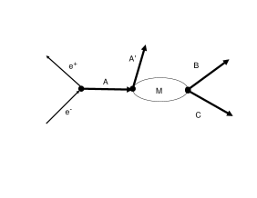
Figure 1: Diagrammatic description of the reactions studied.

The standard expression for the cross section in these cases results in

$$\sigma=\left(\frac{\pi}{E_{e}}\right)^{2}\,G\,\frac{4\,M^{2}\,\Gamma_{ee\gamma}\,\Gamma_{BC}}{\left(P^{2}-M^{2}\right)^{2}+M^{2}\,\Gamma_{M}^{2}}$$ (5)

Here $M$ stands for the monopolium mass, $P$ for the monopolium four-momentum and $G$ is defined by

$$G=\frac{2\,J_{M}+1}{(2\,s_{e}+1)\,\sqrt{(2\,s_{B}+1)\,(2\,s_{C}+1)}},$$

where $J_{M}$ indicates the total angular momentum of monopolium. We recall that the so called unitarity bound, restricts the validity of the Ginzburg-Schiller approximation to $M<m/6$ [7]. The interesting physical situation occurs when $M\ll m$ and consequently, from (2) and the fact that $\omega\sim M$, one gets $g_{eff}\sim g(M/m)\ll 1$, which grants validity to the perturbative approach.

We enter now the computation of the widths $\Gamma$. Taking into account that

$$|\emph{M}_{ee\gamma}|^{2}=\left|<e^{+}\,e^{-}\,|\,\frac{1}{(q^{2}-m_{A}^{2})}\,|\,M,A^{\prime}>\right|^{2}=4\,\pi\,\alpha\,g_{A}^{2}\,g_{A}^{\prime\,2}\,\frac{1}{\left(q^{2}-m_{A}^{2}\right)^{2}}\,\left|\psi_{M}(0)\right|^{2},$$

where $m_{A}$ is the mass of the $A$ particle in Fig. 1. Here $q=(2\,E_{e},\vec{0})$. One obtains,

$$\Gamma_{ee\gamma}=4\,\alpha^{2}\,g_{A}^{2}\,g_{A^{\prime}}^{2}\,\frac{E_{e}^{2}}{\left(4\,E_{e}^{2}-m_{A}^{2}\right)^{2}}\;\left|\psi_{M}(0)\right|^{2}.$$ (6)

Note that the monopolium mass could be small and therefore we have to keep the mass term in the denominator.

We now proceed to calculate

$$\Gamma_{BC}=2\,\pi\,|\emph{M}_{BC}|^{2}\,\rho(E_{BC})$$

Using the standard result [26] we obtain

$$\Gamma_{BC}=\frac{8\,\pi\,g_{B}^{2}\,g_{C}^{2}}{m}\,\left|\psi_{M}(0)\right|^{2},$$ (7)

where the approximation $m\gg m_{B},m_{C}$ has been used. Here $m_{B}$ and $m_{C}$ represent respectively the masses of the $B$ and $C$ particles of Fig. 1.

The cross section, generalized to include the propagation of an unstable particle of width $\Gamma_{A}$ (for us $A=Z_{0}$), becomes

$$\sigma = \frac{2\,G}{(16)^{4}\,\pi^{5}}\,\frac{(\tan\theta_{W})^{2\zeta_{0}}}{\alpha^{3}}\,\frac{M^{2}}{m^{10}}\,|\psi_{M}(0)|^{4}$$ (8)

$$\frac{E_{A^{\prime}}^{2}E_{B}^{2}\,E_{C}^{2}\,(2\,E_{e})^{2}}{\left[(4\,E_{e}^{2}-m_{A}^{2})^{2}+m_{A}^{2}\,\Gamma_{A}^{2}\right]\,\left[(2\,E_{e}-E_{A^{\prime}})^{2}-E_{A^{\prime}}^{2}-M^{2})^{2}+M^{2}\,\Gamma_{M}^{2}\right]}$$

where $\zeta_{0}$ indicates the number of $Z_{0}$’s present among particles $A,\,A^{\prime},\,B$ and $C$ and we have used energy-momentum conservation at the vertex.

In order to go ahead with the calculation, one has to obtain the wave function corresponding to monopolium. This is done and analyzed in the next sections.

3 Monopolium Potential

Our calculation of monopolium reduces to a quantum mechanical bound state calculation which provides us with its mass and its wave function in the relative frame. We will use a static non relativistic approximation and therefore our first step is to define the potential that binds the poles to form monopolium.

We restrict our calculation to the lowest charge monopole, i.e. $N=1$ in the Dirac condition Eq.(1). We regard the monopole as possessing some spatial extension in line with the arguments of Schiff and Goebel [27, 28]. This assumption makes the potential energy of the monopole-antimonopole interaction non-singular when the relative separation goes to zero. Mathematically we describe this feature by means of an exponential cut-off in the interaction potential,

$$V(r)=-g^{2}\,\left(\frac{1-\exp{(-\mu\,r)}}{r}\right).$$ (9)

We fix the cut-off parameter $\mu$ by physical arguments. Eq.(9) has the following properties,

• $r\rightarrow\infty$

  $$V(r)\rightarrow-\frac{g^{2}}{r}$$ (10)

• $r\rightarrow 0$

  $$V(r) \rightarrow -g^{2}\,\mu+\ldots$$ (11)

When the monopole-antimonopole are closest to each other the distance between the corresponding centers $O$ and $O^{\prime}$ is $r_{OO^{\prime}}\sim 2\,r_{m}$, where $r_{m}$ is the pole radius. For our estimates $r_{m}\sim 4\,r_{classical}$ seems reasonable since this choice will allow the monopolium bound state to have very small mass for strong binding. Then

$$\mu=2\,\frac{m}{g^{2}}.$$ (12)

Consequently, the effective potential finally becomes

$$V(r)=-g^{2}\,\frac{1-\exp\left(-2\,\frac{r}{r_{classical}}\right)}{r}.$$ (13)

Note that with our choice, for $r\rightarrow 0$, $V(r)\rightarrow-2m$. Thus, the mass of the bound state becomes the energy over the minimum

$$M=2\,m+E_{binding}.$$ (14)

     

Figure 2: The figure on the left shows the Coulomb and the Coulomb with exponential cut-off potentials. The figure on the right shows energy levels of the Coulomb potential used as energy levels of the cut-off potential. Note that the lowest energy states of the cut-off potential correspond to excited states of the Coulomb potential.

Summarizing, our analysis shows that the cut-off potential is quite close to the Coulomb potential as long as the monopole radius, $r_{m}$ is greater than the classical monopole radius $r_{classical}$. Thus, we shall use the ”magnetic” Coulomb potential (Fig. 2) as our interaction in what follows. However, it is important to note, as will be shown next, that the lowest energy states of the cut-off potential correspond to excited states of the magnetic Coulomb potential (Fig. 2.).

We use a non-relativistic approximation whose validity we will shortly discuss. Solving the Schrödinger equation for monopolium we obtain its binding energy, and therefore the mass of the system is given by [29]

$$M=2\,m-\left(\frac{1}{8\,\alpha}\right)^{2}\,\frac{m}{n^{2}}>0.$$ (15)

where $\alpha=e^{2}=1/137$ and $n$ is the principal quantum number. We see that we can reach zero mass for $n\sim 12$ and therefore for $n>17$ the formula is well defined and describes all values of $M$

$$0\leq M\ \leq 2m$$

.

The monopolium radius is given by

$$\frac{r_{M}}{r_{classical}}=48\alpha^{2}n^{2}.$$ (16)

Now we introduce the size parameter $\rho=r_{M}/r_{classical}$.

By substituting $n^{2}$ from Eq.(16) into Eq.(15), we obtain an equation for the monopolium mass as a function of its size, namely

$$M=m\left(2-\frac{3}{4\rho}\right),$$ (17)

which is plotted in Fig. 3. Although for low values of $\rho$ our approximation becomes worse, we expect, that the soft behavior of the wave function at the origin, allows for order of magnitude estimates. This formula is extremely important in our development because it transmutates principal quantum numbers of the Coulomb potential into mass scales which are crucial to substantiate our scenario.

Figure 3: Mass of the monopolium as a function of the size parameter.The unitarity bound corresponding to $\rho\sim\;0.41$ is shown.

The perturbative expansion of Ginzburg and Schiller used in the calculation of the production process limits, due to unitariry, the maximum value of the ratio of $\frac{M}{m}<1/6$ [7]. We incorporate this external additional requirement to the bound state calculation, which is free from it, by showing the bound in all relevant figures.

Before we continue, a discussion on the validity of the non-relativistic approximation is necessary. Let us therefore analyze how relativistic corrections will affect our calculation. As the monopoles are spin 0 bosons one may describe the system by a Schrödinger type equation and the first corrections to it do not start at order $\beta^{2}$ but at order $\beta^{4}$ (apart from merely the kinetic terms) [30]. These additional terms to order $\beta^{6}$ are,

$$-\frac{\Delta^{4}}{8m^{4}}\;\;;\;-\frac{\Delta^{6}}{16m^{6}}\;;\;\frac{g^{2}}{32m^{5}}[\Delta^{2},[\Delta^{2},\frac{1}{r}]].$$ (18)

They can be treated as perturbations to the Schrödinger equation. In the appendix we give detailed account of the calculation of these corrections.

Figure 4: Shown are the non relativistic $\beta$ (solid), the relativistic bosonic $\beta_{rel}$ (dashed), the first order correction $\beta_{rel}$ (dot-dashed) and the ratio of an upper bound to the order $\beta^{4}$ potential term to the binding energy to order $\beta^{4}$ with correct kinematics (dotted). The unitarity bound is also shown.

We show in Fig. 4 that the correction to the potential energy can be neglected safely, for an order of magnitude estimate, if the kinetic terms are fully taken into account. Moreover, we show that the minimal relativistic correction, consisting in the simplest approximation to the Klein–Gordon equation, namely in incorporating the mass [30], leads to a velocity

$$\beta^{(1)}_{rel}=\frac{\beta}{1+\frac{\beta^{2}}{2}},$$ (19)

which is almost indistinguishable from the more complete given by Eq.(34).

Furthermore, since our potential is cut off for small values of $r$ we expect a slow down of the particles with respect to the conventional Coulomb potential and therefore the non-relativistic treatment is more accurate than in the pure Coulomb case. Moreover, the calculation for the wave function at the origin is less sensitive to the short range behavior of the potential, than the velocity which depends on the slope of the wave function.

4 Cross section estimates

We proceed to use the formalism just developed to describe the production and decay of monopolium. The analysis that follows is physically appealing because the mass of monopolium may be chosen small, much smaller than the monopole mass, thus detection can occur at relatively low energies. Monopolium production is accompanied by radiation, which is also described by the formalism. Furthermore the calculation is easy to perform and physically understandable.

It seems therefore safe to go ahead to calculate the monopolium decay probability as a function of $\rho$. The range of values of $\rho$ : $3/8<\rho<\infty$. Moreover,

$$n=\frac{1}{4\,\alpha}\,\sqrt{\frac{\rho}{3}}$$

and therefore, given a value of $\rho$, one can determine $n$ and this fixes $|\psi(0)|^{2}$, which is what one needs for computing the decay probability. In summary, the calculation seems to be feasible in terms of only one mass scale, the mass of the monopole, $m$, and one parameter, $\rho$.

Let us consider the case when monopolium is produced in its ground state, its wave function will have $\ell=0$. Consequently [29]

$$\psi_{n,0,0}=\frac{1}{a^{3/2}}\,N_{n,0}\,F_{n,0}\left(\frac{2\,r}{n\,a}\right)\,Y^{0}_{0}(\Omega)$$ (20)

with

$$a=\frac{1}{m\,e^{2}}\,\,\,\,;\,\,\,\,N_{n,0}=\frac{2}{n^{2}}\,\sqrt{\frac{(n-1)!}{(n!)^{3}}}$$

and

$$F_{n,0}(x)=e^{-1/2\,x}\,L^{1}_{n-1}(x)\,\,\,\,;\,\,\,\,L^{1}_{n-1}(x)=\sum^{n-1}_{s=0}\,(-1)^{s}\,\frac{(n!)^{2}}{(n-s-1)!\,(s+1)!\,s!}\,x^{s}$$

We need $|\psi_{n,0,0}(0)|$. Then, taking into account that

$$\lim_{x\rightarrow 0}L^{1}_{n-1}(x)=n\,n!\,\,\,;\,\,\,\lim_{x\rightarrow 0}F_{n,0}(x)=n\,n!$$

one has

$$|\psi_{n,0,0}(0)|=\frac{1}{a^{3/2}}\,\frac{2}{n}\,\frac{1}{\sqrt{n}}$$ (21)

The reduced mass of the monopolium system is $m/2$ and the Dirac condition Eq.(1) can be written as

$$g^{2}\,e^{2}=\frac{1}{4}\,\,\,\,\Rightarrow\,\,\,\,\alpha_{g}\,\alpha_{e}=\frac{1}{4}$$

one gets

$$|\psi_{n,0,0}(0)|=\frac{1}{4}\,\left(\frac{m}{2\,\alpha_{e}\,n}\right)^{3/2}$$ (22)

Finally one can write the wave function in terms of the variable $\rho$ to obtain

$$|\psi_{n,0,0}(0)|=\frac{1}{4}\,\left(\frac{2\sqrt{3}\,m}{\sqrt{\rho}}\right)^{3/2}$$ (23)

This is the main ingredient to be included in the expression for the cross section that was computed before.

For spin zero monopoles and being particularly interested in $n$ large and $\ell=0$ , one has $G\sim 1/4$. Replacing the value of the wave function given in (23), and using the relation between $M$ and $\rho$ the cross section, Eq.(8), becomes

$$\sigma = \frac{1}{4^{6}}\frac{27}{32\,\pi^{5}}\,\frac{(\tan\theta_{W})^{2N_{Z_{0}}}}{\alpha^{3}}\,\frac{M^{2}}{m^{4}}\,\left(\frac{4}{3}\,\left(2-\frac{M}{m}\right)\right)^{3}\,$$ (24)

$$\frac{E_{A^{\prime}}^{2}\,E_{B}^{2}\,E_{C}^{2}\,(2\,E_{e})^{2}}{\left[(4\,E_{e}^{2}-m_{A}^{2})^{2}+(m_{A}^{2}\Gamma_{A}^{2}\right]\left[\left((2E_{e}-E_{A^{\prime}})^{2}-E_{A^{\prime}}^{2}-M^{2}\right)^{2}+M^{2}\Gamma_{M}^{2}\right]}.$$

We proceed to describe the case when $A$ is a photon propagator and the external particles $A^{\prime},B$ and $C$ are outgoing photons. Clearly $A=Z_{0}$, $A^{\prime}=B=\gamma,C=\gamma$ also contributes to the $3\gamma$ cross-section. We omit it here for simplicity, since we are just estimating the observability of the process, not its precise magnitude.

In the case under consideration the above cross section becomes,

$$\sigma=\frac{2}{4^{6}\pi^{5}\,\alpha^{3}}\,\frac{M^{2}}{m^{4}}\left(2-\frac{M}{m}\right)^{3}\,\frac{E_{A^{\prime}}^{2}\,E_{B}^{2}\,E_{C}^{2}}{4E_{e}^{2}\;\left[\left((2E_{e}-E_{A^{\prime}})^{2}-E_{A^{\prime}}^{2}-M^{2}\right)^{2}+M^{2}\Gamma_{M}^{2}\right]}\;.$$ (25)

It is evident from the above equation that the cross-section has a resonant structure for

$$E_{A^{\prime}}=E_{e}\left(1-\left(\frac{M}{2\,E_{e}}\right)^{2}\right)$$

In order to maximize the cross-section we will set ourselves on top of the resonant peak and moreover will choose

$$E_{B}=E_{C}=\frac{E_{e}}{2}\left(1+\left(\frac{M}{2\,E_{e}}\right)^{2}\right),$$

which are the values for the energy that maximize the numerator, $E_{B}^{2}E_{C}^{2}$, while satisfying the conservation equations

$$E_{A^{\prime}}+E_{B}+E_{C}=2E_{e}.$$

and

$$\vec{p}_{A^{\prime}}+\vec{p}_{B}+\vec{p}_{C}=\vec{0}$$

These substitutions lead finally to the formula

$$\sigma=\frac{2}{4^{8}\pi^{5}\,\alpha^{3}}\left(\frac{1}{\Gamma_{M}}\right)^{2}\left(\frac{E_{e}}{m}\right)^{4}\left(2-\frac{M}{m}\right)^{3}\left(1-\left(\frac{M}{2E_{e}}\right)^{4}\right)\left(1+\left(\frac{M}{2E_{e}}\right)^{2}\right).$$ (26)

The monopolium width is dominated by the 2 $\gamma$ decay,

$$\Gamma_{M}\sim\Gamma_{BC}(E_{B}=E_{C}=M/2)=\frac{\pi}{8\alpha^{2}}\left(\frac{M}{m}\right)^{3}\,\left(2-\frac{M}{m}\right)^{3/2}M,$$ (27)

with a correction from the $Z_{0}$ decays which is about $30\%$ and which for the purposes of our calculation is irrelevant. Using this width we obtain for the cross section,

$$\sigma\sim\frac{2\alpha}{4^{3}\,\pi^{7}}\frac{m^{2}}{M^{4}}\,\left(\left(\frac{2\,E_{e}}{M}\right)^{4}-1\right)\,\left(1+\left(\frac{M}{2E_{e}}\right)^{2}\right).$$ (28)

The results of our calculation are shown in Figs. 5 and 6 which we now comment. We have two parameters in our calculation, namely the monopole mass $m$ and the monopolium mass $M$. We use in the plots $M$ and the ratio $M/m$. Unitarity imposes a restriction on the latter $M/m<0.15$ as can be seen in Fig. 3. We show data for two values of this ratio, $0.01$, which serves for the purpose of developing our idea and satisfies clearly the unitarity bound, and $0.0001$, which could realize certain cosmological monopole scenarios. The equations are sufficiently simple for any one to play with them. In Fig. 5 we show on the left the cross section at resonance as a function on the mass of the monopolium and for a beam energy just above the monopolium threshold, i.e. $2\,E_{e}=M+0.001\;GeV$. This extreme case leads to low values for the cross section due to the vicinity of the threshold zero (see for comparison the dotted line which is away from the threshold), but is physically very appealing because the photon of the first vertex carries almost no energy and we have a representation of the scalar monopolium decay with two photons appearing back to back with an energy of $M/2$. In this case the photon of the first vertex simply is present to carry away the spin of the intermediate photon but (almost) no energy. We see that the value of the cross section increases as $M/m$ decreases. Thus initially monopolium made of heavier monopoles, for a fixed mass, would be easier to see, if it were not because as shown in the right figure, its width decreases dramatically.

Figure 5: Logarithmic plot of the cross section at resonance (in $fb$) (left) and the monopolium width (in $GeV$) (right) as a function of the monopolium mass (in $GeV$). The vertical lines represent the Tevatron ($M\sim 265\,GeV$)[9] and the LHC ($M\sim 1100\,GeV$) bounds. In the left plot the full lines have been calculated for a beam energy slightly larger than the monopolium mass, $2E_{e}=M+0.001$, to avoid the threshold zero and maximize monopolium production. The dotted line corresponds to a value of $E_{e}$ $100MeV$ above the threshold. The different curves are obtained for the shown values of $M/m=0.01\mbox{ or }0.0001$.

We include the limits of the Tevatron and LHC, which in our way of presenting the data are trivial. Note however, that both in the Tevatron and in LHC, the expected processes are the inverse of the studied here, namely the 2 $\gamma$ (and other mentioned alternatives) of producing monopolium [23, 31].

Let us emphasize at this point looking at the data the interest of what we have named a two scale scenario. The two scales are the monopole mass and the monopolium mass. Our scenario becomes very interesting if the two scales are very different. It is the existence of an additional scale, which is represented in our scheme by the parameter $M/m$, which renders the present investigation exciting. If monopolium is a strongly bound system, it is its relatively low mass which limits the usefulness of the accelerators for monopole physics and not that of the monopole, conventionally assumed to be very large. If monopoles could bind to an almost zero mass bound state we could study monopole physics at relatively low energies.

Figure 6: Logarithmic plot of the cross section at resonance (in $fb$) (left) as a function of beam energy $E_{e}$ for a fixed mass of the monopolium of $1000\;GeV$. The different curves are obtained for the shown values of $M/m=0.01:0.0001$.

In Fig. 6 we show for a fixed monopolium mass how the peak cross section changes with the energy of the beams. We see that the threshold effect is extremely narrow and that the cross section jumps immediately several orders of magnitude. Thus the three photon detection seems much more favorable than the two photon one. The signal is clear: one photon recoiling against two others, whose dynamics describes a resonant structure. Once the threshold effect disappears the cross section is relatively flat with energy.

Let us summarize our findings. In our two scale scenario,

• the studied cross section has a resonant peak (see Eq.(32)) at the monopolium mass $M$;

• the order of magnitude of the cross section is ”almost” beam energy independent, once we are away from the threshold, and is consistent with observability in present day machines [23, 31, 32, 33] for monopolium masses of up to $1000\,GeV$ (see Figs. 5 and 6) and monopole masses only limited by the validity of our theoretical approach;

• a similar analysis can be carried out for $\gamma\,Z_{0}$ and 2$Z_{0}$ decays;

• a similar analysis can be carried out for hadronic production, complicated by the inclusion of the sub-structure of the intervening hadrons.

• Our analysis can generalized to study the $2\,\gamma$, $\gamma\,Z_{0}$ and $2\,Z_{0}$ monopolium production process which should be the dominating mechanism for LHC.

5 Conclusions

We have performed an investigation looking for hints of the so far not seen monopoles. Our working assumption is that monopoles appear strongly bound forming monopolium, a monopole-antimonopole bound state, due to their strong electromagnetic interaction.

We develop a scenario in which monopolium is produced and desintegrates into 2$\gamma$, $\gamma\,Z_{0}$ and 2$Z_{0}$’s. We detail the structure and magnitude of the first of this processes to determine observability. We develop a two energy scale scenario, whose

• low scale is governed by monopolium and we consider for quantitative purposes that it could be reachable by present day machines.

• and whose high energy scale is governed by the monopole mass and arises through the structure of monopolium.

  $$m>>E_{e}.$$

Under these circumstances we can estimate the cross section as a function of the monopolium mass. The monopole mass is determined by the value of the cross section and any mass is attainable, the limitations only arising from the approximations used in our model.

Since at present we can not calculate the monopolium parameters, $M$ and $\Gamma_{M}$, the experimental endeavor is not easy. There are however some features which might simplify the task,

• the resonance peak of the monopolium can be found in four exit channels 3$\gamma$, $2\gamma\,Z_{0}$ and $\gamma\,2\,Z_{0}$’s and $3\,Z_{0}$’s;

• monopolium can be produced in an excited state before it annihilates, thus the annihilation process will be accompanied by a Rydberg radiation spectrum;

• the same processes can be studied hadronically, the only complication arising from the inclusion of the hadron sub-structure.

The calculated values for the cross sections, corresponding to reasonable monopolium mass scenarios, render our calculation interesting and this line of research worth pursuing.

6 Acknowledgement

This work was initiated while VV was visiting the Universidad Nacional de La Plata. He wishes to thank the members of the department for their hospitality. VV was supported by MCYT-FIS2004-05616-C02-01, GV-GRUPOS03/094, a travel grant of the University of Valencia. LNE, HF and CAGC were partially supported by CONICET and ANPCyT Argentina.

Appendix A Appendix: Relativistic corrections

Let us define the relativistic factor $\beta=v/c$ through the equation

$$\beta^{2}=<n\,l\,m_{l}\,m_{s}|\frac{p^{2}}{m^{2}}|n\,l\,m_{l}\,m_{s}>.$$ (29)

It can be easily calculated using the exact expectation value to give [29],

$$\beta=\sqrt{\frac{3}{4\rho}}.$$ (30)

This result, which coincides with the semiclassical treatment and the use of Ehrenfest’s theorems, namely equating the centrifugal and Coulomb forces

$$m\frac{v^{2}}{r}=\frac{e^{2}}{r^{2}}\,\,\,\Rightarrow\,\,\,\frac{p^{2}}{2\,m}=\frac{1}{2}\,\frac{e^{2}}{r}$$

which leads to

$$E=\frac{p^{2}}{2\,m}-\frac{e^{2}}{r}=\frac{p^{2}}{2\,m}-\frac{p^{2}}{m}=-\frac{p^{2}}{2\,m}.$$

This corresponds to equating the absolute values of the kinetic and the binding energies,

$$Kinetic\,\,Energy=|Binding\,\,Energy|,$$ (31)

which gives

$$\frac{p^{2}}{m}=\left(\frac{1}{8\,\alpha}\right)^{2}\,\frac{m}{n^{2}},$$

that gives rise, using Eq.(16), to

$$\frac{p^{2}}{m^{2}}=\frac{3}{4}\,\frac{1}{\rho}.$$

Thus, the non-relativistic calculation is only truly valid for $\rho>3/4$.

One can easily incorporate the kinetic terms in Eq.(18) to the lowest order approximation leading to,

$$m\;(\frac{\beta^{2}}{2}-\frac{\beta^{4}}{8}+\frac{\beta^{6}}{16}+...)$$ (32)

Performing the virial theorem calculation,

$$E_{total}=m\;({1+\frac{\beta^{2}}{2}-\frac{\beta^{4}}{8}+\frac{\beta^{6}}{16}})$$ (33)

and therefore the relativistic velocity turns out to be

$$\beta_{rel}=\frac{\beta}{1+\frac{\beta^{2}}{2}-\frac{\beta^{4}}{8}+\frac{\beta^{6}}{16}}.$$ (34)

The non-relativistic velocity $\beta$ and the relativistic one $\beta_{rel}$ are shown in Fig. 4. Finally the correction to the potential compared to the binding energy becomes,

$$\frac{\frac{g^{2}}{32m^{4}}<[\Delta^{2},[\Delta^{2},\frac{1}{r}]]>}{|E_{binding}|}<\frac{g^{2}}{32}\;\frac{p^{3}}{m^{3}}\approx\frac{137}{128}\beta^{3}_{rel}.$$ (35)

The upper bound is also shown in Fig. 4

References

- [1] P.A.M. Dirac, Proc. Roy. Soc. A133 (1931) 60, Phys. Rev. 74 (1940) 817.
- [2] J. D. Jackson, Classical Electrodynamics, de Gruyter, N.Y. (1982).
- [3] N. Craigie, G. Giacomelli, W. Nahern and Q. Shafi, Theory and detection of magnetic monopoles in gauge theories, World Scientific, Singapore1986.
- [4] T.W.B. Kibble, J. Phys. A 9 (1976) 1387, Phys. Rep. 67 (1980) 183; A. Vilenkin, Phys. Rep. 121 (1985) 263.
- [5] G. Giacomelli and L. Patrizii, hep-ex/0506014.
- [6] A. De Rújula, Nucl. Phys.B435 (1995) 257.
- [7] P.D.B. Martin Collins,A.D. Martin and E.J. Squires, Particle Physics and cosmology, Wiley, N.Y. (1989); K. A. Milton, Rep. Prog. Phys. 69 , 1637 (2006).
- [8] Review of Particle Physics, S. Eidelman et al., Physics Letters B592 2004 1.
- [9] Reviews of Particles Properties, W-M Yao et al., Jour. of Phys. G33 (2006) 1.
- [10] M. J. Mulhearn, Ph.D. Thesis MIT 2004.
- [11] Ya.B Zeldovich and M. Yu. Khlopov, Phys. Lett. 79 (1978) 239.
- [12] C.T. Hill, Nucl. Phys. B224 (1983) 469.
- [13] V.K. Dubrovich. Gravitation and Cosmology, Supplement, 8, 122 (2002)
- [14] E.W. Kolb and M.S. Turner in The Early Universe, Addison-Wesley, New York (1990).
- [15] S. Ahlen et al., Phys. Rev. Lett. 72 (1994) 608
- [16] E.N. Parker, Astrophys. J. 180 (1970) 383; M.S. Turner, E.N. Parker and T. Bogdan, Phys. Rev. D26 (1982) 1296.
- [17] F.C. Adams et al., Phys. Rev. Lett. 70 (1993) 2511.
- [18] P. Bhattacharjee and G. Sigl, Phys. Rev. D51 (1995) 4079.
- [19] J. J. Blanco-Pillado and K. D. Olum, Phys. Rev D60 (1999) 083001.
- [20] V. Vento, Are monopoles hiding in monoplium? astro-ph/0511764.
- [21] N. Hayashida et al., Phys. Rev. Lett. 73, 3491 (1994).
- [22] D.J. Bird et al., Astrophys. J. 424, 491 (1994).
- [23] I.F. Ginzburg and A. Schiller, Phys. Rev. D60, 075016 (1999); Phys. Rev. D60 075016 (2000).
- [24] C. Itzykson and B. Zuber, Quantum Field Theory,(McGraw-Hill, N.Y. 1985)
- [25] S. Weinberg, The Quantum theory of fields (Cambridge University Press, 1996); T.P. Cheng and L.F. Lee, Theory of elementary particles (Oxford University Press, 1982); M.E. Peskin and D.V. Schroeder, An introduction to quantum field theory, by (HarperCollins, 1995).
- [26] J.M. Jauch and F. Rorhlich, The theory of electrons and photons (Springer 1975).
- [27] L.I. Schiff, Phys. Rev. 160 (1967) 1257.
- [28] C.J. Goebel, Quanta, Essays in Theoretical Physics, eds. P.G.O. Freund, C.J. Goebel and Y. Nambu (Chicago, 1970).
- [29] A. Galindo and P. Pascual, Quantum Mechanics (Springer, 1991).
- [30] F.J. Yndurain, Relativistic Quantum Mechanics and Introduction to Field Theory (Springer 1996).
- [31] Yu. Kurochin, I. Satsunkevich and Dz. Shoukavy, Mod. Phys. Lett. bf A21 (2006) 2873.
- [32] I.F. Ginzburg, G.L. Kotkin, V.G. Serbo and V. I. Telnov, Nucl. Inst. and Methods Phys. Res. 205 (1983) 47; I.F. Ginzburg, G.L. Kotkin, S.L. Panfil, V.G. Serbo and V. I. Telnov, Nucl. Inst. and Methods Phys. Res. 219 (1984) 5.
- [33] R. Brinkmann et al., Nucl. Inst. and Methods Phys. Res. A 406 (1998) 13.