Hard exclusive electroproduction of a pion in the backward region

Abstract

We study the scaling regime of pion electroproduction in the backward region, $eN\to e^{\prime}N^{\prime}\pi$. We compute the leading-twist amplitude in the kinematical region, where it factorises into a short-distance matrix element and long-distance dominated nucleon Distribution Amplitudes and nucleon to pion Transition Distribution Amplitudes. Using the chiral limit of the latter, we obtain a first estimate of the cross section, which may be experimentally studied at JLab or Hermes.

I Introduction

In TDApiproton ; Pire:2005mt , we introduced the framework to study backward pion electroproduction

$$\gamma^{\star}(q)N(p_{1})\to N^{\prime}(p_{2})\pi(p_{\pi}),$$ (1)

on a proton (or neutron) target, in the Bjorken regime ($q^{2}$ large and $q^{2}/(2p_{1}.q)$ fixed) in terms of Transition Distribution Amplitudes (TDAs), as well as the reaction $N(p_{1})\bar{N}(p_{2})\to\gamma^{\star}(q)\pi(p_{\pi})$ in the near forward region. This extended the concept of Generalised Parton Distributions. Such an extension of the GPD framework has already been advocated in the pioneering work of Frankfurt:1999fp .

The TDAs involved in the description of Deeply-Virtual Compton Scattering (DVCS) in the backward kinematics

$$\gamma^{\star}(q)N(p_{1})\to N^{\prime}(p_{2})\gamma(p_{\gamma})$$ (2)

and the reaction $N(p_{1})\bar{N}(p_{2})\to\gamma^{\star}(q)\gamma(p_{\gamma})$ in the near forward region were given in Lansberg:2006uh .

This followed the same lines as in TDApigamma , where we have argued that factorisation theorems Collins:1996fb for exclusive processes apply to the case of the reaction $\pi^{-}\,\pi^{+}\,\to\,\gamma^{*}\,\gamma$ in the kinematical regime where the off-shell photon is highly virtual (of the order of the energy squared of the reaction) but the momentum transfer $t$ is small. Besides, in this simpler mesonic case, a perturbative limit may be obtained Pire:2006ik for the $\gamma^{\star}$ to $\rho$ transition. For the $\gamma\to\pi$ one, we have recently shown TDApigamma-appl that experimental analysis of processes such as $\gamma^{\star}\gamma\to\rho\pi$ and $\gamma^{\star}\gamma\to\pi\pi$, which involve the latter TDAs, could be carried out, e.g. the background from the Bremsstrahlung is small if not absent and rates are sizable at present $e^{+}e^{-}$ facilities.

Whereas in the pion to photon case, models used for GPDs Tiburzi:2005nj ; Broniowski:2007fs ; noguera ; GPD_pion could be applied to TDAs since they are defined from matrix elements of the same quark-antiquark operators, this is not obvious for the nucleon to meson or photon TDAs, which are defined from matrix elements of a three-quark operator. Before estimates based on models such as the meson-cloud model Pasquini:2006dv become available, it is important to use model-independent information coming from general theorems. We will use here the constraints for the proton to pion TDAs derived in the chiral limit.

The structure of this paper is the following: first, we recall the necessary kinematics related to hard electroproduction of a pion as well as the definitions of the proton to pion TDAs, which enter the description of the latter process in the backward region; secondly, we establish the limiting constraints on the TDAs in the chiral limit when the final-state pion is soft; thirdly, we calculate the hard contribution for the process; hence, extrapolating the limiting value of the TDAs to the large-$\xi$ region, we give a first evaluation of the unpolarised cross section, by restricting the analysis of the hard part to the sole Efremov-Radyushkin-Brodsky-Lepage (ERBL) region, where all the three quarks struck by the virtual photon have positive light-cone momentum fraction of the target proton.

This analysis is motivated by the experimental conditions Laveissiere:2003jf ; CLAS ; Airapetian:2001iy of JLab and Hermes at moderate electron energies. Related processes with three-quark exchanges in the hard scattering were recently studied in Braun:2006td similarly to what was proposed in Pobylitsa:2001cz .

II Kinematics and definitions

II.1 The electroproduction process $eP\to e^{\prime}P^{\prime}\pi^{0}$

Let us first recall the kinematics for the electron proton collisions (see e.g. Mulders:1990xw ). As usual, we shall work in the one-photon-exchange approximation and consider the differential cross section for $\gamma^{\star}(q)P(p_{1})\to P^{\prime}(p_{2})\pi^{0}(p_{\pi})$ in the center-of-mass frame of the pion and the final-state proton (see the kinematics in Fig. 1). The photon flux $\Gamma$ is defined in the Hand convention to be

$$\Gamma=\frac{\alpha_{em}}{2\pi^{2}}\ \frac{E_{e^{\prime}}}{E_{e}}\ \frac{W^{2}-M^{2}}{2MQ^{2}}\ \frac{1}{1-\epsilon},$$ (3)

with $E_{e}$ the energy of the initial electron in the lab frame (beam energy), $E_{e^{\prime}}$ the one of the scattered electron, $W$ the invariant mass of the $P^{\prime}\pi^{0}$ pair, $M$ the proton mass, $Q^{2}$ the virtuality of the exchanged photon ($Q^{2}=-q^{2}=-(p_{e}-p_{e^{\prime}})^{2}$) and $\epsilon=\frac{1-y}{1-y+y^{2}/2}$ ($y=\frac{q.p_{1}}{p_{e}.p_{1}}$) its linear polarisation parameter. The five-fold differential cross section for the process $eP\to e^{\prime}P^{\prime}\pi^{0}$ can then be reduced to a two-fold one, expressible in the center-of-mass frame of the $P^{\prime}\pi^{0}$ pair, times the flux factor $\Gamma$:

$$\frac{d^{5}\sigma}{dE_{e^{\prime}}d^{2}\Omega_{e}d^{2}\Omega_{\pi}^{\ast}}=\Gamma\ \frac{d^{2}\sigma}{d^{2}\Omega_{\pi}^{\ast}},$$ (4)

where $\Omega_{e}$ is the differential solid angle for the scattered electron in the lab frame, $\Omega_{\pi}^{*}$ is the differential solid angle for the pion in the $P^{\prime}\pi^{0}$ center-of-mass frame, such that $d\Omega_{\pi}^{*}=d\varphi\,d\cos\theta^{*}_{\pi}$. $\theta^{*}_{\pi}$ is defined as the polar angle between the virtual photon and the pion in the latter system. $\varphi$ is the azimuthal angle between the electron plane and the plane of the process $\gamma^{\star}P\to P^{\prime}\pi^{0}$ (hadronic plane) ($\varphi=0$ when the pion is emitted in the half plane containing the outgoing electron, see also Fig. 1).

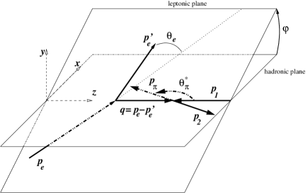
Figure 1: (Backward) electroproduction of a pion on a proton in the center-of-mass frame of the $\gamma^{\star}$ proton.

In general, we have contributions from different polarisations of the photon. For that reason, we define four polarised cross sections, which do not depend on $\varphi$ but only on $W$, $Q^{2}$ and $\theta^{*}_{\pi}$, $d^{2}\sigma_{\mbox{\tiny T}}$, $d^{2}\sigma_{\mbox{\tiny L}}$, $d^{2}\sigma_{\mbox{\tiny TL}}$ and $d^{2}\sigma_{\mbox{\tiny TT}}$. The $\varphi$ dependence is therefore more explicit since

$$\frac{d^{2}\sigma}{d\Omega_{\pi}^{*}} = \frac{d^{2}\sigma_{\mbox{\tiny T}}}{d\Omega_{\pi}^{*}}\ +\ \epsilon\ \frac{d^{2}\sigma_{\mbox{\tiny L}}}{d\Omega_{\pi}^{*}}+\sqrt{2\epsilon(1+\epsilon)}\ \frac{d^{2}\sigma_{\mbox{\tiny TL}}}{d\Omega_{\pi}^{*}}\cos{\varphi}$$ (5)

$$+\ \epsilon\ \frac{d^{2}\sigma_{\mbox{\tiny TT}}}{d\Omega_{\pi}^{*}}\cos{2\varphi}.$$

As we shall show below, at the leading-twist accuracy, the QCD mechanism considered here contributes only to $\frac{d^{2}\sigma_{\mbox{\tiny T}}}{d\Omega_{\pi}^{*}}$ and $\frac{d^{2}\sigma_{\mbox{\tiny TT}}}{d\Omega_{\pi}^{*}}$.

II.2 The subprocess $\gamma^{\star}P\to P^{\prime}\pi^{0}$

In the scaling regime, the amplitude for $\gamma^{\star}P(p_{1})\to P^{\prime}(p_{2})\pi(p_{\pi})$ in the backward kinematics –namely small $u=(p_{\pi}-p_{1})^{2}=\Delta^{2}$ or $\cos\theta^{*}_{\pi}$ close to -1– then involves the TDAs $T(x_{i},\xi,\Delta^{2})$, where $x_{i}$ ($i=1,2,3$) denote the light-cone-momentum fractions carried by participant quarks and $\xi$ is the skewedness parameter such that $2\xi=x_{1}+x_{2}+x_{3}$.

The amplitude is then a convolution of the proton DAs, a perturbatively-calculable-hard-scattering amplitude and the TDAs, defined from the Fourier transform of a matrix element of a three-quark-light-cone operator between a proton and a meson state. We have shown that these TDAs obey QCD evolution equations, which follow from the renormalisation-group equation of the three-quark operator. Their $Q^{2}$ dependence is thus completely under control.

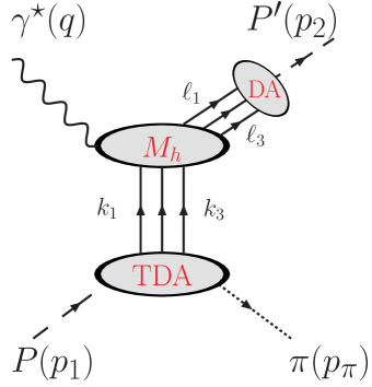
Figure 2: The factorisation of the process $\gamma^{\star}P\to P^{\prime}\;\pi$ into proton-distribution amplitudes (DA), the hard-subprocess amplitude ($M_{h}$) and proton $\to$ pion transition distribution amplitudes (TDA) .

The momenta of the process $\gamma^{\star}P\to P^{\prime}\pi$ are defined as shown in Fig. 1 and Fig. 2. The $z$-axis is chosen along the initial nucleon and the virtual photon momenta and the $x-z$ plane is identified with the collision or hadronic plane (Fig. 1). Then, we define the light-cone vectors $p$ and $n$ ($p^{2}$=$n^{2}$=0) such that $2~{}p.n=1$, as well as $P=\frac{1}{2}(p_{1}+p_{\pi})$, $\Delta=p_{\pi}-p_{1}$ and its transverse component $\Delta_{T}$ ($\Delta_{T}.\Delta_{T}=\Delta_{T}^{2}<0$), which we choose to be along the $x$-axis. From those, we define $\xi$ in an usual way as $\xi=-\frac{\Delta.n}{2P.n}$.

We can then express the momenta of the particles through their Sudakov decomposition and, keeping the first-order corrections in the masses and $\Delta_{T}^{2}$, we have:

$$\begin{split}p_{1}&=(1+\xi)p+\frac{M^{2}}{1+\xi}n,\\ q&\simeq-2\xi\Big{(}1+\frac{(\Delta_{T}^{2}-M^{2})}{Q^{2}}\Big{)}p+\frac{Q^{2}}{2\xi\Big{(}1+\textstyle\frac{(\Delta_{T}^{2}-M^{2})}{Q^{2}}\Big{)}}n,\\ p_{\pi}&=(1-\xi)p+\frac{m_{\pi}^{2}-\Delta_{T}^{2}}{1-\xi}n+\Delta_{T},\end{split}$$

$$\begin{split}p_{2}&\simeq-2\xi\frac{(\Delta_{T}^{2}-M^{2})}{Q^{2}}p\;+\\ &\Big{[}\frac{Q^{2}}{2\xi\Big{(}1+\textstyle\frac{(\Delta_{T}^{2}-M^{2})}{Q^{2}}\Big{)}}-\frac{m_{\pi}^{2}-\Delta_{T}^{2}}{1-\xi}+\frac{M^{2}}{1+\xi}\Big{]}n-\Delta_{T},\\ \Delta&=-2\xi p+\Big{[}\frac{m_{\pi}^{2}-\Delta_{T}^{2}}{1-\xi}-\frac{M^{2}}{1+\xi}\Big{]}n+\Delta_{T}.\end{split}$$ (6)

The polarisation vectors of the virtual photon are chosen to be (in the $P^{\prime}\pi^{0}$ center-of-mass frame):

$$\begin{split}&\varepsilon_{L}(q)\simeq\frac{2\xi(Q^{2}+\Delta_{T}^{2}-M^{2})}{Q^{3}}p+\frac{Q^{3}}{2\xi(Q^{2}+\Delta_{T}^{2}-M^{2})}n,\\ &\varepsilon_{T_{1}}(q)=\varepsilon_{x},~{}~{}\varepsilon_{T_{2}}(q)=\varepsilon_{y}.\end{split}$$ (7)

We also have

$$\begin{split}W^{2}=(p_{1}+q)^{2}\simeq\frac{(1-\xi)Q^{2}}{2\xi}-(\Delta_{T}^{2}-M^{2}),\end{split}$$ (8)

where we have kept the leading term in $Q^{2}$ and the next-to-leading one which does not vanish in the limit $\xi\to 1$. This provides us with the following relation between $\xi$ and $W^{2}$

$$\begin{split}\xi\simeq\frac{Q^{2}}{Q^{2}+2(W^{2}+\Delta_{T}^{2}-M^{2})},\end{split}$$ (9)

which reduces to the usual one, $\xi\simeq\frac{Q^{2}}{Q^{2}+2W^{2}}$, when $M^{2}$ and $\Delta_{T}^{2}$ can be neglected compared to $W^{2}$ (which is not the case in the $\xi\to 1$ limit). Furthermore, we have the exact relation

$$\begin{split}x_{B}=\frac{Q^{2}}{2p_{1}.q}=\frac{Q^{2}}{W^{2}+Q^{2}-M^{2}},\end{split}$$ (10)

which gives

$$\begin{split}\xi\simeq\frac{x_{B}}{2-x_{B}}.\end{split}$$ (11)

Finally, we have (neglecting the pion mass):

$$\begin{split}\Delta_{T}^{2}=\frac{1-\xi}{1+\xi}u-2M^{2}\frac{1-\xi}{(1+\xi)^{2}}\xi.\end{split}$$ (12)

In Ref. TDApiproton , we have defined the leading-twist proton to pion $P\to\pi$ transition distribution amplitudes from the Fourier transform of the matrix element

$$\begin{split}\langle\pi|\,\epsilon^{ijk}{q}^{i^{\prime}}_{\alpha}(z_{1}n)\,[z_{1};z_{0}]_{i^{\prime},i}\,{q}^{j^{\prime}}_{\beta}(z_{2}n)\,[z_{2};z_{0}]_{j^{\prime}j}\,{q}^{k^{\prime}}_{\gamma}(z_{3}n)\\ \times[z_{3};z_{0}]_{k^{\prime}k}\,|P\rangle.\end{split}$$ (13)

The brackets $[z_{i};z_{0}]$ in Eq. (13) account for the insertion of a path-ordered gluonic exponential along the straight line connecting an arbitrary initial point $z_{0}n$ and a final one $z_{i}n$:

$$\begin{split}[z_{i};z_{0}]\equiv{\rm P\ exp\,}\biggl{[}ig\!\!\!\int_{0}^{1}\!\!\!dt\,(z_{i}-z_{0})n_{\mu}A^{\mu}(n[tz_{i}+(1-t)z_{0}])\biggr{]}\end{split}$$ (14)

which provide the QCD-gauge invariance for such non-local operator and equal unity in a light-like (axial) gauge.

The leading-twist TDAs for the $p\to\pi^{0}$ transition, $V^{p\pi^{0}}_{i}\!\!(x_{i},\xi,\Delta^{2})$, $A^{p\pi^{0}}_{i}\!\!(x_{i},\xi,\Delta^{2})$ and $T^{p\pi^{0}}_{i}\!\!(x_{i},\xi,\Delta^{2})$ are defined here as :

$$4{\cal F}\Big{(}\langle\pi^{0}(p_{\pi})|\,\epsilon^{ijk}u^{i}_{\alpha}(z_{1}n)u^{j}_{\beta}(z_{2}n)d^{k}_{\gamma}(z_{3}n)\,|P(p_{1},s_{1})\rangle\Big{)}=$$ (15)

$$i\frac{f_{N}}{f_{\pi}}\Big{[}V^{p\pi^{0}}_{1}(p\!\!\!/C)_{\alpha\beta}(N^{+})_{\gamma}+A^{p\pi^{0}}_{1}(p\!\!\!/\gamma^{5}C)_{\alpha\beta}(\gamma^{5}N^{+})_{\gamma}+T^{p\pi^{0}}_{1}(\sigma_{p\mu}C)_{\alpha\beta}(\gamma^{\mu}N^{+})_{\gamma}$$

$$+M^{-1}V^{p\pi^{0}}_{2}(p\!\!\!/C)_{\alpha\beta}(\Delta\!\!\!/\!_{T}N^{+})_{\gamma}+M^{-1}A^{p\pi^{0}}_{2}(p\!\!\!/\gamma^{5}C)_{\alpha\beta}(\gamma^{5}\Delta\!\!\!/\!_{T}N^{+})_{\gamma}+M^{-1}T^{p\pi^{0}}_{2}(\sigma_{p\Delta_{T}}C)_{\alpha\beta}(N^{+})_{\gamma}$$

$$+M^{-1}T^{p\pi^{0}}_{3}(\sigma_{p\mu}C)_{\alpha\beta}(\sigma^{\mu\Delta_{T}}N^{+})_{\gamma}+M^{-2}T^{p\pi^{0}}_{4}(\sigma_{p\Delta_{T}}C)_{\alpha\beta}(\Delta\!\!\!/\!_{T}N^{+})_{\gamma}\;\Big{]},$$

where $\sigma^{\mu\nu}=1/2[\gamma^{\mu},\gamma^{\nu}]$ with $\sigma^{p\mu}=p_{\nu}\sigma^{\nu\mu}$,…, $C$ is the charge conjugation matrix and $N^{+}$ is the large component of the nucleon spinor ($N=(n\!\!\!/p\!\!\!/+p\!\!\!/n\!\!\!/)N=N^{-}+N^{+}$ with $N^{+}\sim\sqrt{p_{1}^{+}}$ and $N^{-}\sim\sqrt{1/p_{1}^{+}}$). $f_{\pi}$ is the pion decay constant ($f_{\pi}=131$ MeV) and $f_{N}$ has been estimated through QCD sum rules to be of order $5.2\cdot 10^{-3}$ GeV² CZ . All the TDAs $V_{i}$, $A_{i}$ and $T_{i}$ are dimensionless. Note that the first three terms in (15) are the only ones surviving the limit $\Delta_{T}\to 0$.

III The soft-pion limit

We now derive the general limit of these three contributing TDAs at $\Delta_{T}=0$ in the soft-pion limit, when $\xi$ gets close to 1 (see also Lansberg:2007se ). In that limit, the soft-meson theorem AD derived from current algebra apply Pobylitsa:2001cz , which allow us to express these 3 TDAs in terms of the 3 Distribution Amplitudes (DAs) of the corresponding baryon. In the case of the proton DA CZ , $V^{p}(x_{i})$, $A^{p}(x_{i})$, $T^{p}(x_{i})$ are defined such as

$$\begin{split}4{\cal F}_{DA}\Big{(}\langle 0|\epsilon_{ijk}u^{i}_{\alpha}(z_{1}n)&u^{j}_{\beta}(z_{2}n)d^{k}_{\gamma}(z_{3}n)|P(p,s)\rangle\Big{)}=f_{N}\times\\ \Big{[}&V^{p}(x_{i})(p\!\!\!/C)_{\alpha\beta}(\gamma^{5}N^{+})_{\gamma}\\ +&A^{p}(x_{i})(p\!\!\!/\gamma^{5}C)_{\alpha\beta}N^{+}_{\gamma}\\ +&T^{p}(x_{i})(\sigma_{p\mu}\,C)_{\alpha\beta}(\gamma^{\mu}\gamma^{5}N^{+})_{\gamma}\Big{]},\end{split}$$ (16)

with ${\cal F}_{DA}\equiv(p.n)^{3}\int^{\infty}_{-\infty}\Pi_{j}\frac{dz_{j}}{(2\pi)^{3}}e^{i\Sigma_{k}x_{k}z_{k}p.n}$ where $p$ is here the proton momentum.

Inspired by Pobylitsa:2001cz , which considered the related case of the distribution amplitude of the proton-meson system, we use the soft pion theorems AD to write:

$$\langle\pi^{a}(p_{\pi})|{\cal O}|N(p_{1},s_{1})\rangle=-\frac{i}{f_{\pi}}\langle 0|[Q^{a}_{5},{\cal O}]|N(p_{1},s_{1})\rangle$$ (17)

$$\!\!\!\!+\frac{ig_{A}}{4f_{\pi}p_{1}.p_{\pi}}\sum_{s^{\prime}_{1}}\bar{N}(p_{1},s^{\prime}_{1})p\!\!\!/_{\pi}\gamma_{5}\tau^{a}N(p_{1},s_{1})\langle 0|{\cal O}|N(p_{1},s^{\prime}_{1})\rangle$$

The second term, which takes care of the nucleon pole term, does not contribute at threshold and will not be considered in the following.

For the transition $p\to\pi^{0}$, $Q^{a}_{5}=Q^{3}_{5}$ and ${\cal O}=u_{\alpha}u_{\beta}d_{\gamma}$. Since the commutator of the chiral charge $Q_{5}$ with the quark field $\psi$ ($\tau^{a}$ being the Pauli matrix)

$$[Q_{5}^{a},\psi]=-\frac{\tau^{a}}{2}\gamma^{5}\psi\;,$$ (18)

the first term in the rhs of Eq. (III) gives three terms from $(\gamma^{5}u)_{\alpha}u_{\beta}d_{\gamma}$, $u_{\alpha}(\gamma^{5}u)_{\beta}d_{\gamma}$ and $u_{\alpha}u_{\beta}(\gamma^{5}d)_{\gamma}$. The corresponding multiplication by $\gamma^{5}$ (or $(\gamma^{5})^{T}$ when it acts on the index $\beta$) on the vector and axial structures of the DA (Eq. (16)) gives two terms which cancel and the third one, which remains, is the same as the one for the TDA up to the modification that on the DA decomposition, $p$ is the proton momentum, whereas for the TDA one, $p$ is the light-cone projection of $P$, ${\it i.e.}$ half the proton momentum if $\xi=1$. This introduces a factor $2\xi$ in the relations between the 2 DAs $A^{p}$ and $V^{p}$ and the 2 TDAs $V^{p\pi^{0}}_{1}$ and $A^{p\pi^{0}}_{1}$, which is canceled though by the factor one half in Eq. (18).

To what concerns the tensorial structure multiplying $T^{p}$, the three terms are identical at leading-twist accuracy and corresponds to the structure multiplying $T^{p\pi^{0}}_{1}$, this gives a factor 3. Finally, an extra factor $(4\xi)^{-1}$ appears when one goes to the momentum space Lansberg:2007se . We eventually have at $\Delta_{T}=0$:

$$V^{p\pi^{0}}_{1}(x_{1},x_{2},x_{3},\xi,\Delta^{2})=\frac{V^{p}}{4\xi}\Big{(}\frac{x_{1}}{2\xi},\frac{x_{2}}{2\xi},\frac{x_{3}}{2\xi}\Big{)},$$

$$A^{p\pi^{0}}_{1}(x_{1},x_{2},x_{3},\xi,\Delta^{2})=\frac{A^{p}}{4\xi}\Big{(}\frac{x_{1}}{2\xi},\frac{x_{2}}{2\xi},\frac{x_{3}}{2\xi}\Big{)},$$ (19)

$$T^{p\pi^{0}}_{1}(x_{1},x_{2},x_{3},\xi,\Delta^{2})=\frac{3T^{p}}{4\xi}\Big{(}\frac{x_{1}}{2\xi},\frac{x_{2}}{2\xi},\frac{x_{3}}{2\xi}\Big{)}.$$

Note the factor $\frac{1}{2\xi}$ in the argument of the DA in Eq. (III). We refer to Lansberg:2007se for a complete discussion. Indeed, for the TDAs, the $x_{i}$ are defined with respect to $p$ ( see e.g. ${\cal F}\equiv(p.n)^{3}\int^{\infty}_{-\infty}\Pi_{j}\frac{dz_{j}}{(2\pi)^{3}}e^{i\Sigma_{k}x_{k}z_{k}p.n}$) which tends to $\frac{p_{1}}{2}$ when $\xi\to 1$. Therefore, they vary within the interval $[-2,2]$, whereas for the DAs, the momentum fractions are defined with respect to the proton momentum $p_{1}$ and vary between 0 and 1.

Our results are comparable to the ones for the proton-pion DAs obtained in Braun:2006td . Finally, it is essential to note that these limiting values are not zero, unlike for some GPDs. Hence, we find it reasonable to conjecture that these expressions give the right order of magnitude of the TDAs for quite large values of $\xi$ (say $\xi\geq 0.5$) in a first estimate of cross sections.

IV Hard-amplitude calculation

At leading order in $\alpha_{s}$, the amplitude ${\cal M}^{\lambda}_{s_{1}s_{2}}$ for $\gamma^{\star}(q,\lambda)P(p_{1},s_{1})\to P^{\prime}(p_{2},s_{2})\pi^{0}(p_{\pi})$ reads

$$\begin{split}&{\cal M}^{\lambda}_{s_{1}s_{2}}=-i\frac{(4\pi\alpha_{s})^{2}\sqrt{4\pi\alpha_{em}}f_{N}^{2}}{54f_{\pi}Q^{4}}\times\\ &\Big{[}\underbrace{\bar{u}(p_{2},s_{2})\varepsilon\!\!\!/(\lambda)\gamma^{5}u(p_{1},s_{1})}_{{\cal S}^{\lambda}_{s_{1}s_{2}}}\\ &~{}~{}~{}~{}~{}~{}~{}~{}~{}~{}~{}~{}~{}~{}~{}~{}~{}~{}~{}~{}~{}~{}\times\underbrace{\int\limits^{1+\xi}_{-1+\xi}\!\!\!d^{3}x\int\limits_{0}^{1}\!\!d^{3}y\Bigg{(}2\sum\limits_{\alpha=1}^{7}T_{\alpha}+\sum\limits_{\alpha=8}^{14}T_{\alpha}\Bigg{)}}_{{\cal I}}\\ &-\underbrace{\varepsilon(\lambda)_{\mu}\Delta_{T,\nu}\bar{u}(p_{2},s_{2})(\sigma^{\mu\nu}+g^{\mu\nu})\gamma^{5}u(p_{1},s_{1})}_{{\cal S^{\prime}}^{\lambda}_{s_{1}s_{2}}}\\ &~{}~{}~{}~{}~{}~{}~{}~{}~{}~{}~{}~{}~{}~{}~{}~{}~{}~{}~{}\times\underbrace{\int\limits^{1+\xi}_{-1+\xi}\!\!\!d^{3}x\int\limits_{0}^{1}\!\!d^{3}y\Bigg{(}2\sum\limits_{\alpha=1}^{7}T^{\prime}_{\alpha}+\sum\limits_{\alpha=8}^{14}T^{\prime}_{\alpha}\Bigg{)}}_{{\cal I^{\prime}}}\Big{]},\end{split}$$ (20)

where the coefficient $T_{\alpha}$ and $T^{\prime}_{\alpha}$$(\alpha=1,...,14)$ are functions of $x_{i}$,$y_{j}$,$\xi$ and $\Delta^{2}$ and are given in Table (LABEL:tab:coeff_funct). In general, we have 21 diagrams: we have not drawn 7 others which differ only to the 7 first ones by a permutation between the $u$-quark lines $1$ and $2$. The symmetry of the integration domain and of the DAs and TDAs with respect to the changes $x_{1}\leftrightarrow x_{2}$ and $y_{1}\leftrightarrow y_{2}$ therefore tells us that they give the same contributions as the 7 first diagrams. They are accounted for by a factor 2 in the last equation.

The integrals in Eq. (LABEL:eq:ampl-bEPM1) are understood with two delta-functions insuring momentum conservation:

$$\begin{split}&\int d^{3}x\equiv\int dx_{1}dx_{2}dx_{3}\delta(2\xi-x_{1}-x_{2}-x_{3})\end{split}$$ (21)

and

$$\begin{split}&\int d^{3}y\equiv\int dy_{1}dy_{2}dy_{3}\delta(1-y_{1}-y_{2}-y_{3}).\end{split}$$ (22)

The expression in Eq. (LABEL:eq:ampl-bEPM1) is to be compared with the leading-twist amplitude for the baryonic-form factor CZ

$$\begin{split}&{\cal M}^{\lambda}\propto-i\bar{u}(p_{2})\varepsilon\!\!\!/(\lambda)u(p_{1})\frac{\alpha_{s}^{2}f_{N}^{2}}{Q^{4}}\\ &\int\limits_{0}^{1}d^{3}x\int\limits_{0}^{1}d^{3}y\Bigg{(}2\sum\limits_{\alpha=1}^{7}T^{p}_{\alpha}(x_{i},y_{j},\xi,t)+\sum\limits_{\alpha=8}^{14}T^{p}_{\alpha}(x_{i},y_{j},\xi,t)\Bigg{)}.\end{split}$$ (23)

The factors $T^{p}_{\alpha}$ are very similar to the $T_{\alpha}$ obtained here.

Table 1: 14 of the 21 diagrams contributing to the hard-scattering amplitude with their associated coefficient $T_{\alpha}$ and $T^{\prime}_{\alpha}$. The seven first ones with $u$-quark lines inverted are not drawn. The crosses represent the virtual-photon vertex.

$\alpha$		$T_{\alpha}$	$T^{\prime}_{\alpha}$
1		$\frac{-Q_{u}(2\xi)^{2}[(V_{1}^{p\pi^{0}}-A_{1}^{p\pi^{0}})(V^{p}-A^{p})+4T^{p\pi^{0}}_{1}T^{p}+2\frac{\Delta^{2}_{T}}{M^{2}}T^{p\pi^{0}}_{4}T^{p}]}{(2\xi-x_{1}-i\epsilon)^{2}(x_{3}-i\epsilon)(1-y_{1})^{2}y_{3}}$	$\frac{-Q_{u}(2\xi)^{2}[(V_{2}^{p\pi^{0}}-A_{2}^{p\pi^{0}})(V^{p}-A^{p})+2(T^{p\pi^{0}}_{2}+T^{p\pi^{0}}_{3})T^{p}]}{(2\xi-x_{1}-i\epsilon)^{2}(x_{3}-i\epsilon)(1-y_{1})^{2}y_{3}}$
2		$0$	$0$
3		$\frac{Q_{u}(2\xi)^{2}[4T^{p\pi^{0}}_{1}T^{p}+2\frac{\Delta^{2}_{T}}{M^{2}}T^{p\pi^{0}}_{4}T^{p}]}{(x_{1}-i\epsilon)(2\xi-x_{2}-i\epsilon)(x_{3}-i\epsilon)y_{1}(1-y_{1})y_{3}}$	$\frac{Q_{u}(2\xi)^{2}[2(T^{p\pi^{0}}_{2}+T^{p\pi^{0}}_{3})T^{p}]}{(x_{1}-i\epsilon)(2\xi-x_{2}-i\epsilon)(x_{3}-i\epsilon)y_{1}(1-y_{1})y_{3}}$
4		$\frac{-Q_{u}(2\xi)^{2}[(V_{1}^{p\pi^{0}}-A_{1}^{p\pi^{0}})(V^{p}-A^{p})]}{(x_{1}-i\epsilon)(2\xi-x_{3}-i\epsilon)(x_{3}-i\epsilon)y_{1}(1-y_{1})y_{3}}$	$\frac{-Q_{u}(2\xi)^{2}[(V_{2}^{p\pi^{0}}-A_{2}^{p\pi^{0}})(V^{p}-A^{p})]}{(x_{1}-i\epsilon)(2\xi-x_{3}-i\epsilon)(x_{3}-i\epsilon)y_{1}(1-y_{1})y_{3}}$
5		$\frac{Q_{u}(2\xi)^{2}[(V_{1}^{p\pi^{0}}+A_{1}^{p\pi^{0}})(V^{p}+A^{p})]}{(x_{1}-i\epsilon)(2\xi-x_{3}-i\epsilon)(x_{3}-i\epsilon)y_{1}(1-y_{2})y_{3}}$	$\frac{Q_{u}(2\xi)^{2}[(V_{2}^{p\pi^{0}}+A_{2}^{p\pi^{0}})(V^{p}+A^{p})]}{(x_{1}-i\epsilon)(2\xi-x_{3}-i\epsilon)(x_{3}-i\epsilon)y_{1}(1-y_{2})y_{3}}$
6		$0$	$0$
7		$\frac{-Q_{d}(2\xi)^{2}[2(V_{1}^{p\pi^{0}}V^{p}+A_{1}^{p\pi^{0}}A^{p})]}{(x_{1}-i\epsilon)(2\xi-x_{3}-i\epsilon)^{2}y_{1}(1-y_{3})^{2}}$	$\frac{-Q_{d}(2\xi)^{2}[2(V_{2}^{p\pi^{0}}V^{p}+A_{2}^{p\pi^{0}}A^{p})]}{(x_{1}-i\epsilon)(2\xi-x_{3}-i\epsilon)^{2}y_{1}(1-y_{3})^{2}}$
8		$0$	$0$
9		$\frac{-Q_{u}(2\xi)^{2}[(V_{1}^{p\pi^{0}}-A_{1}^{p\pi^{0}})(V^{p}-A^{p})+4T^{p\pi^{0}}_{1}T^{p}+2\frac{\Delta^{2}_{T}}{M^{2}}T^{p\pi^{0}}_{4}T^{p}]}{(2\xi-x_{1}-i\epsilon)^{2}(x_{2}-i\epsilon)(1-y_{1})^{2}y_{2}}$	$\frac{-Q_{u}(2\xi)^{2}[(V_{2}^{p\pi^{0}}-A_{2}^{p\pi^{0}})(V^{p}-A^{p})+2(T^{p\pi^{0}}_{2}+T^{p\pi^{0}}_{3})T^{p}]}{(2\xi-x_{1}-i\epsilon)^{2}(x_{2}-i\epsilon)(1-y_{1})^{2}y_{2}}$
10		$\frac{-Q_{u}(2\xi)^{2}[(V_{1}^{p\pi^{0}}+A_{1}^{p\pi^{0}})(V^{p}+A^{p})+4T^{p\pi^{0}}_{1}T^{p}+2\frac{\Delta^{2}_{T}}{M^{2}}T^{p\pi^{0}}_{4}T^{p}]}{(x_{1}-i\epsilon)(2\xi-x_{2}-i\epsilon)^{2}y_{1}(1-y_{2})^{2}}$	$\frac{-Q_{u}(2\xi)^{2}[(V_{2}^{p\pi^{0}}+A_{2}^{p\pi^{0}})(V^{p}+A^{p})+2(T^{p\pi^{0}}_{2}+T^{p\pi^{0}}_{3})T^{p}]}{(x_{1}-i\epsilon)(2\xi-x_{2}-i\epsilon)^{2}y_{1}(1-y_{2})^{2}}$
11		$0$	$0$
12		$\frac{Q_{d}(2\xi)^{2}[(V_{1}^{p\pi^{0}}+A_{1}^{p\pi^{0}})(V^{p}+A^{p})]}{(x_{1}-i\epsilon)(x_{2}-i\epsilon)(2\xi-x_{3}-i\epsilon)y_{1}(1-y_{2})y_{2}}$	$\frac{Q_{d}(2\xi)^{2}[(V_{2}^{p\pi^{0}}+A_{2}^{p\pi^{0}})(V^{p}+A^{p})]}{(x_{1}-i\epsilon)(x_{2}-i\epsilon)(2\xi-x_{3}-i\epsilon)y_{1}(1-y_{2})y_{2}}$
13		$\frac{-Q_{d}(2\xi)^{2}[4T^{p\pi^{0}}_{1}T^{p}+2\frac{\Delta^{2}_{T}}{M^{2}}T^{p\pi^{0}}_{4}T^{p}]}{(x_{1}-i\epsilon)(2\xi-x_{1}-i\epsilon)(x_{2}-i\epsilon)y_{1}(1-y_{2})y_{2}}$	$\frac{-Q_{d}(2\xi)^{2}[2(T^{p\pi^{0}}_{2}+T^{p\pi^{0}}_{3})T^{p}]}{(x_{1}-i\epsilon)(2\xi-x_{1}-i\epsilon)(x_{2}-i\epsilon)y_{1}(1-y_{2})y_{2}}$
14		$\frac{Q_{d}(2\xi)^{2}[(V_{1}^{p\pi^{0}}-A_{1}^{p\pi^{0}})(V^{p}-A^{p})]}{(x_{1}-i\epsilon)(2\xi-x_{1}-i\epsilon)(x_{2}-i\epsilon)y_{1}y_{2}(1-y_{3})}$	$\frac{Q_{d}(2\xi)^{2}[(V_{2}^{p\pi^{0}}-A_{2}^{p\pi^{0}})(V^{p}-A^{p})]}{(x_{1}-i\epsilon)(2\xi-x_{1}-i\epsilon)(x_{2}-i\epsilon)y_{1}y_{2}(1-y_{3})}$

V Cross-section estimate for unpolarised protons

When $\xi$ is large, the ERBL region covers most of the integration domain. This corresponds to the emission of three quarks of positive light-cone-momentum fraction off the target proton. Therefore it is legitimate to approximate the cross section only from the ERBL region. As a consequence, the integration on the momentum fractions contained in the TDAs between $-1+\xi$ and ${1+\xi}$ (see Eq. (LABEL:eq:ampl-bEPM1)) can be converted into one between 0 and 1 by a change of variable and can be carried out straightforwardly.

On the other hand, we have at our disposal a reasonable estimation of the TDAs $V_{1}^{p\pi^{0}}$, $A_{1}^{p\pi^{0}}$ and $T_{1}^{p\pi^{0}}$ in the large-$\xi$ region and for vanishing $\Delta_{T}$ thanks to the soft pion limit (see section III). As a consequence, we have all the tools needed for a first evaluation of the unpolarised cross section for $\gamma^{\star}P\to P^{\prime}\pi^{0}$ for large $\xi$ and when $\Delta^{2}_{T}$ is vanishing.

The differential cross section for unpolarised protons in the proton-pion center-of-mass frame is calculated as usual from the averaged-squared amplitudes, ${|{\cal M}_{i}|}^{2}$ ($i=T,L,TT,LT$):

$$\begin{split}\frac{d\sigma_{i}}{d\Omega^{*}_{\pi}}=&\frac{1}{64\pi^{2}W^{2}}\frac{\sqrt{(p_{\pi}.p_{2})^{2}-m_{\pi}^{2}M^{2})}}{\sqrt{(p_{1}.q)^{2}+M^{2}Q^{2})}}{|{\cal M}_{i}|}^{2}\\ \simeq&\frac{W^{2}-M^{2}}{64\pi^{2}W^{2}\sqrt{(W^{2}+M^{2}+Q^{2})^{2}-4W^{2}M^{2}}}{|{\cal M}_{i}|}^{2}.\end{split}$$ (24)

The ${|{\cal M}_{i}|}^{2}$ are obtained from squaring and summing (resp. averaging) ${\cal M}^{\lambda}_{s_{1}s_{2}}$ over the final (resp. initial) proton helicities with given appropriate combinations of the photon helicity $\lambda$ Mulders:1990xw . The expression of ${\cal M}^{\lambda}_{s_{1}s_{2}}$ are obtained from Eq. (LABEL:eq:ampl-bEPM1).

For vanishing $\Delta^{2}_{T}$, the spinorial structure ${\cal S}^{\lambda}_{s_{1}s_{2}}$

$$\begin{split}\bar{u}(p_{2},s_{2})\varepsilon\!\!\!/(\lambda)\gamma^{5}u(p_{1},s_{1})\end{split}$$ (25)

only survives. To obtain ${|{\cal M}_{T}|}^{2}$, we square the latter and sum over the proton helicities and the transverse polarisations of the photon, it gives a factor $\frac{2(1+\xi)Q^{2}}{\xi}$. On the other hand, ${|{\cal M}_{L}|}^{2}$, vanishes at the leading-twist accuracy, as in the nucleon-form-factor case. The same is true for $|{{\cal M}_{LT}}|^{2}$ and ${|{\cal M}_{TT}|}^{2}$ since the $x$ and $y$ direction are not distinguishable when $\Delta^{2}_{T}$ is vanishing.

Contrariwise, if we wanted to consider the spinorial structure ${\cal S^{\prime}}^{\lambda}_{s_{1}s_{2}}$ – arising when $\Delta^{2}_{T}\neq 0$ –

$$\begin{split}\varepsilon(\lambda)_{\mu}\Delta_{T,\nu}\bar{u}(p_{2},s_{2})(\sigma^{\mu\nu}+g^{\mu\nu})\gamma^{5}u(p_{1},s_{1})\;,\end{split}$$ (26)

$|{{\cal M}_{TT}}|^{2}$, and thus $\frac{d\sigma_{TT}}{d\Omega^{*}_{\pi}}$, would not be zero and the cross section would show a $\cos 2\varphi$ dependence.

The remaining part still to be considered is now entirely contained in the factor $\cal I$ of Eq. (LABEL:eq:ampl-bEPM1) for which we need to choose parametrisations for the DAs and the TDAs. For the sake of coherence, we shall choose the same parametrisation for both. Since the asymptotic limit Lepage:1980fj $V^{p}(x_{i})=T^{p}(x_{i})=\varphi_{as}=120x_{1}x_{2}x_{3}$ and $A(x_{i})=0$ is known to give a vanishing proton-form factor and the wrong sign to the neutron one, we shall not use it.

Note, however, that the isospin relations between the TDAs $V^{p\pi^{0}}_{1}$, $A^{p\pi^{0}}_{1}$ and $T^{p\pi^{0}}_{1}$ differ from those between the DAs; the factor 3 in Eq. (III) clearly illustrates this fact. Therefore, whereas the asymptotic limit choices give a vanishing proton form factor due to a full cancellation between the 14-diagram contributions, the resulting expression will not vanish here even for the asymptotic DAs and TDAs derived in the soft limit.

Yet, we shall rather consider the more reasonable choices of V. L. Chernyak and A. R. Zhitnitsky CZ (noted CZ) based on an analysis of QCD sum rules.

Therefore, we take for the DAs:

$$\begin{split}V^{p}(x_{i})&=\varphi_{as}[11.35(x_{1}^{2}+x_{2}^{2})+8.82x_{3}^{2}-1.68x_{3}-2.94],\\ A^{p}(x_{i})&=\varphi_{as}[6.72(x_{2}^{2}-x_{1}^{2})],\\ T^{p}(x_{i})&=\varphi_{as}[13.44(x_{1}^{2}+x_{2}^{2})+4.62x_{3}^{2}+0.84x_{3}-3.78],\\ \end{split}$$ (27)

and for the limiting value of the TDAs

$$\begin{split}V^{p\pi^{0}}\!\!&=\frac{\varphi_{as}}{2^{5}\xi^{4}}[\frac{11.35}{(2\xi)^{2}}(x_{1}^{2}+x_{2}^{2})+\frac{8.82}{(2\xi)^{2}}x_{3}^{2}-\frac{1.68}{2\xi}x_{3}-2.94],\\ A^{p\pi^{0}}\!\!&=\frac{\varphi_{as}}{2^{5}\xi^{4}}[\frac{6.72}{(2\xi)^{2}}(x_{2}^{2}-x_{1}^{2})],\\ T^{p\pi^{0}}\!\!&=\frac{3\varphi_{as}}{2^{5}\xi^{4}}[\frac{13.44}{(2\xi)^{2}}(x_{1}^{2}+x_{2}^{2})+\frac{4.62}{(2\xi)^{2}}x_{3}^{2}+\frac{0.84}{2\xi}x_{3}-3.78].\\ \end{split}$$ (28)

With this choice, we get the following analytic result valid at large values of $\xi$:

$$\begin{split}\frac{d\sigma}{d\Omega^{*}_{\pi}}&\Big{|}_{\theta^{*}_{\pi}=\pi}=\frac{0.389\alpha_{em}\alpha_{s}^{4}f_{N}^{4}\pi^{3}(W^{2}-M^{2})}{f^{2}_{\pi}W^{2}\sqrt{(W^{2}+M^{2}+Q^{2})^{2}-4W^{2}M^{2}}}\\ &\times\frac{4.5\times 10^{7}(1+\xi)}{Q^{6}\xi}.\end{split}$$ (29)

The algebraic factors come from the DA and TDA parametrisation (Eqs. (27) & (28)). For $\xi=0.8$, we have the $Q^{2}$ dependence of $\frac{d\sigma}{d\Omega^{*}_{\pi}}\big{|}_{\theta^{*}_{\pi}=\pi}$ shown in Fig. 3 for $\alpha_{s}=0.4$.

Figure 3: $\frac{d\sigma}{d\Omega^{*}_{\pi}}\big{|}_{\theta^{*}_{\pi}=\pi}$ for $\xi=0.8$ as function of $Q^{2}$.

Our lack of knowledge of the TDAs unfortunately prevents us from comparing our results with existing data Laveissiere:2003jf . Indeed these data at $Q^{2}=1$GeV² are mostly in the resonance region ($W<1.5$ GeV) except for the large $W$ tail of the distribution, which however correspond to small values of the skewedness parameter ($\xi<.3$). We thus need a realistic model for the $p\to\pi$ TDAs at smaller values of $\xi$ before discussing present data. The issue is more favorable at higher energies, where higher values of $\xi$ can be attained above the resonance region, as for instance at HERMES and with CEBAF at 12 GeV  JLAB12 . Our calculation of the cross section, in an admittedly quite narrow range of the parameters, can thus serve as a reasonable input to the feasibility study of backward pion electroproduction at CEBAF at 12 GeV, in the hope to reach the scaling regime, in which we are interested.

The corresponding results for the asymptotic choice are three order of magnitude smaller. This shows how sensitive the amplitude is with respect to non-perturbative input of the DAs. This has to be paralleled with the perfect cancellations in the proton-form-factor calculation in this limit. The breaking of the isospin relations for the TDAs prevents some of these cancellations, but the full cross section is still shrunk down, whereas the CZ choice gives a much larger contribution as expected.

VI Conclusion

Hard-exclusive electroproduction of a meson in the backward region thus opens a new window in the understanding of hadronic physics in the framework of the collinear-factorisation approach of QCD. Of course, the most important and most difficult problem to solve, in order to extract reliable precise information on the $p\to\pi$ Transition Distribution Amplitudes from an incomplete set of observables such as cross sections and asymmetries, is to develop a realistic model for the TDAs. This is the subject of non-perturbative studies such as, e.g. lattice simulations. We have derived the limit of these TDAs when the pion momentum is small and we have provided a first estimate of the cross section in the kinematical regime which should be accessed at JLab at 12 GeV.

This estimate, which is unfortunately reliable only in a restricted kinematical domain, also shows an interesting sensitivity to the underlying model for the proton DA. Beside information about the pion content in protons through the TDAs, backward pion electroproduction is therefore also likely to bring us information about the protons DAs themselves.

Finally, it is worthwhile to note that the analysis presented here could be easily extended to $ep\to e^{\prime}n\pi^{+}$, $ep\to e^{\prime}\Delta^{0}\pi^{+}$, $ep\to e^{\prime}\Delta^{+}\pi^{0}$, $ep\to e^{\prime}\Delta^{++}\pi^{-}$ and similar reactions with a neutron target, for which data can also be expected private2 .

References

• (1) B. Pire and L. Szymanowski, Phys. Lett. B 622 (2005) 83 [arXiv:hep-ph/0504255]. Note that a multiplicative factor $4\xi^{2}$ is missing in Eq. 23 of the published version.
• (2) B. Pire and L. Szymanowski, PoS HEP2005 (2006) 103 [arXiv:hep-ph/0509368].
• (3) L. L. Frankfurt, P. V. Pobylitsa, M. V. Polyakov and M. Strikman, Phys. Rev. D 60 (1999) 014010 [arXiv:hep-ph/9901429].
• (4) J. P. Lansberg, B. Pire and L. Szymanowski, Nucl. Phys. A 782 (2007) 16 [arXiv:hep-ph/0607130].
• (5) B. Pire and L. Szymanowski, Phys. Rev. D 71 (2005) 111501 [arXiv:hep-ph/0411387].
• (6) J. C. Collins, L. Frankfurt and M. Strikman, Phys. Rev. D 56 (1997) 2982 [arXiv:hep-ph/9611433].
• (7) B. Pire, M. Segond, L. Szymanowski and S. Wallon, Phys. Lett. B 639 (2006) 642 [arXiv:hep-ph/0605320].
• (8) J. P. Lansberg, B. Pire and L. Szymanowski, Phys. Rev. D 73 (2006) 074014 [arXiv:hep-ph/0602195].
• (9) B. C. Tiburzi, Phys. Rev. D 72 (2005) 094001 [arXiv:hep-ph/0508112].
• (10) W. Broniowski and E. Ruiz Arriola, arXiv:hep-ph/0701243.
• (11) S. Noguera, private communication.
• (12) W. Broniowski and E. Ruiz Arriola, Phys. Lett. B 574 (2003) 57 [arXiv:hep-ph/0307198]. L. Theussl, et al., Eur. Phys. J. A 20 (2004) 483 [arXiv:nucl-th/0211036]; A. E. Dorokhov and L. Tomio, Phys. Rev. D 62 (2000) 014016 [arXiv:hep-ph/9803329]; F. Bissey, et al., Phys. Lett. B 547 (2002) 210 [arXiv:hep-ph/0207107]. F. Bissey, et al., Phys. Lett. B 587 (2004) 189 [arXiv:hep-ph/0310184].
• (13) B. Pasquini and S. Boffi, Phys. Rev. D 73 (2006) 094001 [arXiv:hep-ph/0601177].
• (14) G. Laveissiere et al. [JLab Hall A Collaboration], Phys. Rev. C 69 (2004) 045203 [arXiv:nucl-ex/0308009].
• (15) M. Ungaro et al. [CLAS Collaboration], Phys. Rev. Lett.  97 (2006) 112003 [arXiv:hep-ex/0606042]; R. W. Gothe [CLAS Collaboration], AIP Conf. Proc.  814 (2006) 278.
• (16) A. Airapetian et al. [HERMES Collaboration], Phys. Lett. B 535 (2002) 85 [arXiv:hep-ex/0112022].
• (17) V. M. Braun, D. Y. Ivanov, A. Lenz and A. Peters, Phys. Rev.  D 75 (2007) 014021 [arXiv:hep-ph/0611386].
• (18) P. V. Pobylitsa, M. V. Polyakov and M. Strikman, Phys. Rev. Lett.  87 (2001) 022001 [arXiv:hep-ph/0101279].
• (19) P. J. Mulders, Phys. Rept.  185 (1990) 83.
• (20) V. L. Chernyak and A. R. Zhitnitsky, Phys. Rept.  112, 173 (1984);
• (21) J. P. Lansberg, B. Pire and L. Szymanowski, to appear in PRD, rapid communication. [arXiv:0710.1267].
• (22) S. Adler and R. Dashen, Current Algebras, Benjamin, New York, 1968.
• (23) G. P. Lepage and S. J. Brodsky, Phys. Rev. D 22 (1980) 2157.
• (24) J. Roche, C. E. Hyde-Wright, B. Michel, C. Munoz Camacho, et al. [Hall A Collaboration], arXiv:nucl-ex/0609015.
• (25) M. Garçon, F.X. Girod, private communication.