Low Intermediate Scales for Leptogenesis in Supersymmetric
${\bf SO(10)}$ Grand Unified Theories

Abstract

A low intermediate scale within minimal supersymmetric $SO(10)$ GUTs is a desirable feature to accommodate leptogenesis. We explore this possibility in models where the intermediate gauge symmetry breaks spontaneously by (a) doublet Higgs scalars and also (b) by triplets. In both scenarios gauge coupling unification requires the scale of left-right symmetry breaking ($M_{R}$) to be close to the unification scale. This will entail unnaturally small neutrino Yukawa couplings to avoid the gravitino problem and allow successful leptogenesis. We point out that any one of three options – threshold corrections due to the mass spectrum near the unification scale, gravity induced non-renormalizable operators near the Planck scale, or presence of additional light Higgs multiplets – can permit unification along with much lower values of $M_{R}$ as required for leptogenesis. In the triplet model, independent of these corrections, we find a lower bound on the intermediate scale, $M_{R}>10^{9}$ GeV, arising from the requirement that the theory must remain perturbative at least upto the GUT scale. We show that in the doublet model $M_{R}$ can even be in the TeV region which, apart from permitting resonant leptogenesis, can be tested at LHC and ILC.

I Introduction

An area where the standard model based on the group $SU(3)_{C}\times SU(2)_{L}\times U(1)_{Y}\equiv{\cal G}_{std}$ merits improvement is the origin of parity violation. The most natural extension that addresses this issue is the left-right symmetric model in which the gauge group is enlarged to $SU(3)_{C}\times SU(2)_{L}\times SU(2)_{R}\times U(1)_{(B-L)}\equiv{\cal G}_{LR}$ lr . Here, the left-handed fermions transform nontrivially under $SU(2)_{L}$ and are singlet under $SU(2)_{R}$, while it is the converse for the right-handed fermions. It is then possible to extend the definition of parity of the Lorentz group to all particles and ensure that the theory is invariant under the transformation of parity. Spontaneous breaking of the group $SU(2)_{R}$ would trigger violation of parity in the low energy theory. It is also possible to break the parity symmetry spontaneously by the vacuum expectation value ($vev$) of a gauge singlet scalar field which has odd parity dpar . In either case, parity violation at low energy originates from some spontaneous symmetry breaking at high energy.

The simplest grand unified theory (GUT) that includes the left-right symmetric extension of the standard model is based on the gauge group $SO(10)$ and has been studied very widely so10 . In recent times there is renewed interest in the $SO(10)$ GUT stemming from the predictability of the minimal structure of the models min1 . These minimal $SO(10)$ models with the most economical choices of Higgs scalars have several interesting features min1 ; min2 ; min3 ; min4 . Here we show that the possibility of leptogenesis  lept ; lepto can also be accommodated in these models. From an analysis of gauge coupling unification, we determine the scale of left-right symmetry breaking, which is intimately related to a successful prediction of leptogenesis in these models. An apparent obstacle arises in the following form: either these models do not allow any intermediate mass scales or the intermediate left-right symmetry breaking scale comes out to be large ($\sim 10^{15}$ GeV). To implement leptogenesis, on the other hand, the left-right symmetry breaking scale has to be much lower. We exhibit several alternate possibilities which may provide a way out from this impasse.

There are two broad classes of minimal $SO(10)$ models: those with only doublet Higgs scalars (Model I) and the conventional left-right symmetric model including triplet Higgs scalars (Model II). In both versions, a bi-doublet Higgs scalar ($\phi\equiv(1,2,2,0)$ under ${\cal G}_{LR}$) gives mass to the charged fermions and also a Dirac mass to the neutrinos f1 . In an $SO(10)$ GUT, this bi-doublet $\phi$ belongs to the representation ${\bf 10,120}$ or ${\bf 126}$. Usually a ${\bf 10}$ representation is chosen. However, for correct fermion mass relations gj , a ${\bf\overline{126}}$ representation containing the field $\phi^{\prime}\equiv\{15,2,2\}$ under the group $SU(4)_{C}\times SU(2)_{L}\times SU(2)_{R}\equiv{\cal G}_{PS}$ is often chosen.

The main differences between Models I and II lie in the Higgs scalar that breaks the left-right symmetry and the generation of neutrino masses. Lepton number violation in these models arises from the Higgs scalars that break the $B-L$ symmetry and hence the left-right symmetry. The origin of leptogenesis is also different in these two models. There is a natural mechanism of resonant leptogenesis in Model I (see below) while Model II has other advantages.

In Model I, the left-right symmetric group ${\cal G}_{LR}$ is broken by an $SU(2)_{R}$ doublet Higgs scalar $\chi_{R}\equiv(1,1,2,-1)$ when its neutral component acquires a $vev$ $\langle\chi^{\circ}_{R}\rangle\sim v_{R}$. Left-right parity implies the presence of an $SU(2)_{L}$ doublet Higgs scalar $\chi_{L}\equiv(1,2,1,-1)$. The $vev$ of the neutral component of this field, $\langle\chi^{\circ}_{L}\rangle\sim v_{L}$, in addition to $\langle\phi\rangle$, breaks the electroweak symmetry.

In this Model there is an extra singlet fermion, $S$, that combines with the neutrinos and a new type of see-saw mechanism is operational valle . There are several interesting features associated with this. The one relevant here is that the singlet fermions can be almost degenerate with the neutrinos, leading to resonant leptogenesis naturally in this scenario new .

In Model II, an $SU(2)_{R}$ triplet Higgs scalar $\bar{\Delta}_{R}\equiv(1,1,3,2)$ breaks the left-right symmetric group ${\cal G}_{LR}$. When the neutral component acquires a $vev$, $\langle{\bar{\Delta}}^{\circ}_{R}\rangle\sim v_{R}$, it gives Majorana masses to the right-handed neutrinos breaking lepton number by two units. When the bi-doublet Higgs scalar $\phi$ breaks the electroweak symmetry, this leads to the small see-saw neutrino mass see-saw . Due to left-right parity, there is also an $SU(2)_{L}$ triplet Higgs scalar $\bar{\Delta}_{L}\equiv(1,3,1,2)$. Although these scalars have a mass at the parity breaking scale $M_{R}$, the $vev$ of the neutral component of this field is extremely tiny and can give small Majorana masses to the left-handed neutrinos leading to the type II see-saw mechanism, explanation of large neutrino mixings through $b-\tau$ unification, and parameterization of all fermion masses, mixings, and CP-violation. Decays of the right-handed neutrinos or the left-handed triplet Higgs scalars can generate a lepton asymmetry at the scale $M_{R}$. With high left-right symmetry breaking scale and asymptotic parity conservation, Model II is truly a renormalizable high scale SUSY $SO(10)$ theory of fermion masses and mixings min1 ; min2 ; min3 ; goh .

The Majorana mass of right-handed neutrinos is given by $M_{N}\sim\tilde{f}v_{R}$, where $\tilde{f}$ is the Yukawa coupling. The right-handed neutrino mass-scale controls leptogenesis as well as light neutrino masses and, in particular, a value around $10^{9}$ GeV or lower is favored by the ‘gravitino constraint’ discussed below. Since $\tilde{f}$ does not affect the experimentally measured charged fermion masses at low energies, one can assign any value to it, leaving the left-right symmetry breaking scale unrestricted. However, such a low RH neutrino mass is likely to give too large contributions to the left-handed neutrino masses through the see-saw mechanism, contradicting experimental observation. The main motivation of the see-saw mechanism was to avoid arbitrarily small Yukawa couplings, so we shall assume the value of $\tilde{f}$ to be of order unity f2 .

While considering leptogenesis in the minimal supersymmetric $SO(10)$ GUTs, the potential problem grav arising from the overclosure of the universe by gravitinos (and its adverse influence on the successful Big Bang Nucleosynthesis predictions) must be taken into account. This requires the reheating temperature, $T_{RH}$, to be less than $\sim 10^{8}$ GeV. Since leptogenesis takes place just below the scale of left-right symmetry breaking, $M_{R}>T_{RH}$ can make models inconsistent with the above or at least unnatural. However, Model I may still be consistent because it offers the alternative of resonant leptogenesis.

Using renormalization group (RG) equations, in the following sections we examine for both Models whether gauge coupling unification at all allows a low left-right symmetry breaking scale which would make successful leptogenesis viable.

Models I and II have the same symmetry breaking chain:

$$SO(10) \stackrel{{\scriptstyle 210~{}(M_{U})}}{{\longrightarrow}} SU(3)_{C}\times SU(2)_{L}\times SU(2)_{R}\times U(1)_{B-L}$$

$$\stackrel{{\scriptstyle 16~{}{\rm or}~{}126~{}(M_{R})}}{{\longrightarrow}} SU(3)_{C}\times SU(2)_{L}\times U(1)_{Y}$$

$$\stackrel{{\scriptstyle 10~{}(M_{Z})}}{{\longrightarrow}} SU(3)_{C}\times U(1)_{Q}$$

At the GUT scale, the symmetry is broken by the vacuum expectation value of a ${\bf 210}$ dimensional representation of $SO(10)$. The ${\bf 210}$ has a singlet under the subgroup ${\cal G}_{PS}$, i.e., $\{1,1,1\}$, which is odd under parity. When this field acquires a $vev$, $SO(10)$ is broken to ${\cal G}_{PS}$ and D-parity is also spontaneously broken (i.e., $g_{2L}\neq g_{2R}$). To keep D-parity intact at this level we have to look elsewhere. The $SO(10)$ 210 also contains a {15,1,1} under ${\cal G}_{PS}$ which is D-parity even. This is the field to which the $vev$ must be ascribed to get the desired symmetry breaking to ${\cal G}_{LR}$ while keeping D-parity intact.

The left-right symmetry, ${\cal G}_{LR}$, is broken by the $vev$ of the fields $F+\bar{F}$, where $F$ is a ${\bf{16}(\equiv\bf{\Gamma})}$ dimensional representation for Model I and a ${\bf 126}$ dimensional representation for Model II. Finally, the electroweak symmetry breaking takes place by the $vev$ of a 10-plet of $SO(10)$. In the minimal models under consideration, there are no other Higgs representations.

The simplicity of the minimal supersymmetric $SO(10)$ GUT allows several interesting predictions. With some standard assumptions it is possible to determine the mass scales involved in the symmetry breaking. Below, we shall show that one-loop renormalization group evolution leads to left-right symmetry breaking and unification scales,

$$M_{R}^{0}\simeq 1.3\times 10^{16}~{}{\rm GeV},~{}~{}~{}~{}M_{U}^{0}\simeq 2.9\times 10^{16}~{}{\rm GeV}.$$ (1)

$M_{R}^{0}$ and $M_{U}^{0}$ are already very close. But, the situation worsens when two-loop RG contributions are included and we find that no intermediate scales are allowed at all below the unification scale. All this makes leptogenesis unnatural in this class of models. We suggest some possible remedies.

In this paper we show that inclusion of GUT-threshold effects, gravitational corrections through $\rm{dim}.5$ operators, or presence of additional light fields near $M_{R}$, can lower the intermediate scale, bringing it even to the range of a few TeV in the doublet model. Thus, in this model, the gravitino constraint can be easily satisfied leading to successful resonant leptogenesis at low scales. In addition, the signatures of right handed gauge bosons, ($W_{R}^{\pm}$, $Z_{R}$), and new Higgs scalars can be tested at the LHC and ILC. In the triplet model, on the other hand, even though the GUT threshold corrections are much larger, we derive a bound on the intermediate scale, $M_{R}>10^{9}$ GeV arising out of the requirement of perturbation theory to be valid, due to which the scale cannot be reduced further. With this lower bound on $M_{R}$ the triplet model emerges genuinely as a high scale supersymmetric theory for successful description of fermion masses and mixings.

This paper is organised in the following manner. In Sec.II we discuss renormalization group equations and origins of threshold and Planck scale effects. In Sec.III we show how low intermediate scales are obtained in the doublet model and $M_{R}$ can be lowered upto $5\times 10^{9}$ GeV in the triplet model. The perturbative lower bound on $M_{R}$ is derived in Sec.IV. After making brief remarks on fermion masses and light scalars in the SUSY $SO(10)$ model in Sec.V, we summarise the results and state our conclusions in Sec.VI.

II Renormalization group equations

In this section, first we present the RG equations including (a) two-loop beta functions, (b) threshold effects, and (c) contributions from non-renormalizable interactions appearing at the Planck scale. Later we show that, with the minimal particle content and in the absence of effects due to (b) and (c), at the one-loop level Models I and II imply a high scale for $M_{R}$ near $M_{U}$ but when two-loop effects are taken into account even that is excluded.

II.1 General formulation

The RG equations with one f3 intermediate scale, $M_{R}$, between $M_{U}$ and $M_{Z}$ are:

$${1\over\alpha_{i}(M_{Z})} = {1\over\alpha_{i}(M_{R})}+{a_{i}\over 2\pi}\ln{M_{R}\over M_{Z}}+\Theta_{i}-\Delta_{i},$$ (2)

$${1\over\alpha_{i}(M_{R})} = {1\over\alpha_{i}(M_{U})}+{a^{\prime}_{i}\over 2\pi}\ln{M_{U}\over M_{R}}+\Theta^{\prime}_{i}-\Delta^{\prime}_{i}-\Delta_{i}^{(gr)},$$

where $i$ runs over the different gauge couplings. In the R.H.S. of eqs. (2) and (LABEL:eqA.2), the second and third terms represent one- and two-loop contributions, respectively, with

$$\Theta_{i} = {1\over 4\pi}\sum_{j}B_{ij}\ln{\alpha_{j}(M_{R})\over\alpha_{j}(M_{Z})},$$

$$\Theta^{\prime}_{i} = {1\over 4\pi}\sum_{j}B^{\prime}_{ij}\ln{\alpha_{j}(M_{U})\over\alpha_{j}(M_{R})},$$

$$B_{ij} = {b_{ij}\over a_{j}},\,B^{\prime}_{ij}={b^{\prime}_{ij}\over a^{\prime}_{j}}.$$ (4)

The one- and two-loop coefficients ($a_{j},a^{\prime}_{j},b_{ij},b^{\prime}_{ij}$) for specific scenarios are given later. Between $M_{Z}$ and $M_{R}$ the indices $i,j\subset{\cal G}_{std}$ while above $M_{R}$ one has $i,j\subset{\cal G}_{LR}$.

The $\Delta_{i}$ include SUSY threshold effects and intermediate scale threshold effects at $M_{R}$,

$$\Delta_{i}=\Delta^{(S)}_{i}+\Delta^{(R)}_{i},$$

while $\Delta^{\prime}_{i}$ includes the same at the unification scale $M_{U}$. They are represented as carena ; baer ; langacker ; parida1 ,

$$\Delta_{i}^{(S)} = \frac{1}{2\pi}\Sigma_{\alpha}b_{i}^{\alpha}\ln{{M^{\alpha}}\over M_{S}}\equiv\frac{b_{i}}{2\pi}\ln{{M_{i}}\over{M_{S}}},\;\;\;b_{i}=\Sigma_{\alpha}b_{i}^{\alpha},$$

$$\Delta_{i}^{(R)} = \frac{1}{2\pi}\Sigma_{\beta}{c}_{i}^{\beta}\ln{{M^{\beta}}\over M_{R}}\equiv\frac{b^{\prime}_{i}}{2\pi}\ln{{M_{i}}\over{M_{R}}},\;\;\;b^{\prime}_{i}=\Sigma_{\beta}{c}_{i}^{\beta},$$

$$\Delta^{\prime}_{i} = \frac{1}{2\pi}\Sigma_{\gamma}{d}_{i}^{\gamma}\ln{{M^{\gamma}}\over M_{U}}\equiv\frac{b^{\prime\prime}_{i}}{2\pi}\ln{{M_{i}}\over{M_{U}}},\;\;\;b^{\prime\prime}_{i}=\Sigma_{\gamma}{d}_{i}^{\gamma}.~{}~{}~{}~{}$$ (5)

$$\Delta_{i}^{(gr)} = -{{\epsilon}_{i}\over{\alpha}_{G}},i=BL,2L,2R,3C.$$ (6)

Here the indices $\alpha,\beta$ and $\gamma$ signify the particle components of $SO(10)$ representations spread around the SUSY scale $M_{S}$, the $SU(2)_{R}\times U(1)_{B-L}$ breaking scale $M_{R}$, and the $SO(10)$ breaking scale $M_{U}$, respectively.

The definition of effective mass parameters at the SUSY scale $M_{S}$ through the first of eqs. (5) introduced by Carena, Pokorski and Wagner carena has been generalised to study GUT-threshold effects by Langacker and Polonsky langacker in SUSY $SU(5)$ and in ref. parida1 to study intermediate breaking in SUSY $SO(10)$. The effective mass parameters defined through these relations are not arbitrary. Logarithm of each of them is a well defined linear combination of logarithms of actual particle masses (heavy or superheavy) spread around the respective thresholds. Hence, in principle, it is possible to express them in terms of the parameters of the superpotential. The actual relationship would vary from model to model depending upon the type and number of representations used in driving the spontaneous symmetry breaking of SUSY $SO(10)$ to the low energy theory.

In the absence of unnatural mass spectra, the particles are expected to be a few times heavier or lighter than the associated threshold scale which would result in the effective mass parameters bearing a similar relationship to that scale.

The term $\Delta^{gr}_{i}$ represents the effect of $\rm{dim}.5$-operators which may be induced at the Planck scale. These operators modify the boundary condition at $M_{U}$ as shafi ; parpat ,

$$\alpha_{2L}(M_{U})(1+\epsilon_{2L})=\alpha_{2R}(M_{U})(1+\epsilon_{2R})=\alpha_{BL}(M_{U})(1+\epsilon_{BL})=\alpha_{3C}(M_{U})(1+\epsilon_{3C})=\alpha_{G}.~{}~{}~{}~{}~{}$$ (7)

Here, $\alpha_{G}=g^{2}(M_{U})/{4\pi}$ is the GUT fine-structure constant. The impact of various contributions in eqs. (5) and (6) in lowering the intermediate scale in SUSY $SO(10)$ GUTs will be discussed in detail in subsequent sections.

Using eqs. (2) - (6) one obtains for the mass scales parida1 ,

$$\ln{M_{R}\over M_{Z}} = {1\over(AB^{\prime}-A^{\prime}B)}[(AL_{S}-A^{\prime}L_{\Theta})+(A^{\prime}J_{2}-AK_{2})-{2\pi\over\alpha_{G}}(A\epsilon^{\prime\prime}-A^{\prime}\epsilon^{\prime})+(A^{\prime}J_{\Delta}-AK_{\Delta})],$$ (8)

$$\ln{M_{U}\over M_{Z}} = {1\over(AB^{\prime}-A^{\prime}B)}[(B^{\prime}L_{\Theta}-BL_{S})+(BK_{2}-B^{\prime}J_{2})-{2\pi\over\alpha_{G}}(B^{\prime}\epsilon^{\prime}-B\epsilon^{\prime\prime})+(BK_{\Delta}-B^{\prime}J_{\Delta})],$$ (9)

where

$$L_{S} = {2\pi\over\alpha(M_{Z})}\left(1-{8\over 3}{\alpha(M_{Z})\over\alpha_{S}(M_{Z})}\right),$$

$$L_{\Theta} = {2\pi\over\alpha(M_{Z})}\left(1-{8\over 3}\sin^{2}\Theta_{W}(M_{Z})\right),$$

$$A = a^{\prime}_{2R}+{2\over 3}a^{\prime}_{BL}-{5\over 3}a^{\prime}_{2L},$$

$$B = {5\over 3}(a_{Y}-a_{2L})-A,$$

$$A^{\prime} = \left(a^{\prime}_{2R}+{2\over 3}a^{\prime}_{BL}+a^{\prime}_{2L}-{8\over 3}a^{\prime}_{3C}\right),$$

$$B^{\prime} = {5\over 3}a_{Y}+a_{2L}-{8\over 3}a_{3C}-A^{\prime}.$$ (10)

$$J_{2} = 2\pi\left[\Theta^{\prime}_{2R}+{2\over 3}\Theta^{\prime}_{BL}-{5\over 3}\Theta^{\prime}_{2L}+{5\over 3}(\Theta_{Y}-\Theta_{2L})\right],$$

$$K_{2} = 2\pi\left[\Theta^{\prime}_{2R}+{2\over 3}\Theta^{\prime}_{BL}+\Theta^{\prime}_{2L}-{8\over 3}\Theta^{\prime}_{3C}\right.+\left.{5\over 3}\Theta_{Y}+\Theta_{2L}-{8\over 3}\Theta_{3C}\right],$$

$$\epsilon^{\prime} = \epsilon_{2R}+{2\over 3}\epsilon_{BL}-{5\over 3}\epsilon_{2L},$$

$$\epsilon^{\prime\prime} = \epsilon_{2L}+\epsilon_{2R}+{2\over 3}\epsilon_{BL}-{8\over 3}\epsilon_{3C},$$

$$J_{\Delta} = -2\pi\left[\Delta^{\prime}_{2R}+{2\over 3}\Delta^{\prime}_{BL}-{5\over 3}\Delta^{\prime}_{2L}+{5\over 3}(\Delta_{Y}-\Delta_{2L})\right],$$

$$K_{\Delta} = -2\pi\left[\Delta^{\prime}_{2R}+{2\over 3}\Delta^{\prime}_{BL}+\Delta^{\prime}_{2L}-{8\over 3}\Delta^{\prime}_{3C}\right.\left.+{5\over 3}\Delta_{Y}+\Delta_{2L}-{8\over 3}\Delta_{3C}\right].$$ (11)

II.2 The minimal SUSY $SO(10)$ models

In this subsection we apply the RG evolution detailed above to the specific minimal $SO(10)$ models keeping only the one- and two-loop contributions in eqs. (2) - (11).

The symmetry breaking proceeds through three steps. (a) In the first step, the $SO(10)$ symmetry is broken at $M_{U}$ by the $vev$ of a ${\bf 210}$ multiplet. As noted earlier, it is chosen to be along the neutral component of $\{15,1,1\}$ under ${\cal G}_{PS}$ which is even under D-parity dpar . Thus, the gauge symmetry is broken to ${\cal G}_{LR}$ and, with unbroken D-parity, left-right discrete symmetry survives preserving $g_{2L}=g_{2R}$. (b) In the second step, in Model I (the doublet model), the $vev$ of the neutral component of ${\overline{\chi_{R}}}\subset{\bf\overline{16}}$ which transforms as $(1,1,2,-1)$ under ${\cal G}_{LR}$ breaks $SU(2)_{R}\times U(1)_{B-L}\to U(1)_{Y}$ at $M_{R}$. The left-handed doublets $\chi_{L}(1,2,1,-1)\oplus{\overline{\chi_{L}}}(1,2,1,1)$ and other components of $\chi_{R}(1,1,2,-1)\oplus{\overline{\chi_{R}}}(1,1,2,1)$ not absorbed by the RH gauge bosons remain light with masses around the intermediate scale $M_{R}$. (c) Finally, the standard doublet Higgs contained in the bi-doublet $\phi(1,2,2,0)\subset{\bf 10}$ drives the symmetry breaking of ${\cal G}_{std}\to SU(3)_{C}\times U(1)_{em}$ at the electroweak scale. For simplicity, in the remainder of this section it is assumed that the supersymmetry scale, $M_{S}$, is the same as $M_{Z}$. In Model II (the triplet model) steps (a) and (c) remain identical. In step (b), i.e., the breaking of ${\cal G}_{LR}$, the $vev$ is assigned to the neutral component of a field $\overline{\Delta}_{R}\equiv$ (1,1,3,2) contained in a ${\bf\overline{126}}$. In this alternative, the left-handed triplets $\Delta_{L}(1,3,1,-2)\oplus{\overline{\Delta_{L}}}(1,3,1,2)$ contained in the ${\bf 126}$ and ${\bf\overline{126}}$ as well as other components of $\Delta_{R}(1,1,3,-2)\oplus{\overline{\Delta_{R}}}(1,1,3,2)$ not absorbed by the RH gauge bosons remain light and contribute to the gauge coupling evolution from $M_{R}$.

One major difficulty in obtaining the parity conserving ${\cal G}_{LR}$ intermediate symmetry originates from the mass spectra predictions in the triplet model with certain colored Higgs components of $G_{PS}$ multiplets in $\{15,3,1\}+\{15,1,3\}\subset{\bf 210}$ being at the $M_{R}$ scale min3 . We note that a similar difficulty also arises in the minimal doublet model unless these states are made superheavy through the presence of additional $SO(10)$ Higgs representations or non-renormalizable terms in the superpotential as discussed in Sec.IV. Assuming that these additional scalars are made superheavy, our RG analysis applies with the minimal particle content between $M_{Z}$ to $M_{U}$ as described above.

For Model I, the MSSM one- and two-loop beta-function coefficients below the scale $(M_{R})$ are given by,

$$\left(\begin{array}[]{c}a_{Y}\\ a_{2L}\\ a_{3C}\end{array}\right)=\left(\begin{array}[]{c}{33\over 5}\\ 1\\ -3\end{array}\right),~{}~{}~{}~{}b_{ij}=\left(\begin{array}[]{ccc}{199\over 25}&{27\over 5}&{88\over 5}\\ {9\over 5}&25&24\\ {11\over 5}&9&14\end{array}\right),i,j\subset{\cal G}_{std}.$$ (21)

Above $M_{R}$ till $M_{U}$ the beta-function coefficients are

$$\left(\begin{array}[]{c}a^{\prime}_{BL}\\ a^{\prime}_{2L}\\ a^{\prime}_{2R}\\ a^{\prime}_{3C}\end{array}\right)=\left(\begin{array}[]{c}9\\ 2\\ 2\\ -3\end{array}\right),~{}~{}b^{\prime}_{ij}=\left(\begin{array}[]{cccc}{23/2}&{27/2}&{27/2}&{8}\\ {9/2}&{32}&{3}&{24}\\ {9/2}&{3}&{32}&{24}\\ {1}&{9}&{9}&{14}\end{array}\right),i,j\subset{\cal G}_{LR}.$$ (34)

Using $\alpha_{S}(M_{Z})=0.1187$, $\alpha(M_{Z})=1/127.9$, and $\sin^{2}\Theta_{W}=0.2312$, the one-loop solutions yield

$$M_{R}^{0}=1.3\times 10^{16}~{}{\rm GeV~{}~{}~{}~{}~{},}~{}~{}~{}~{}~{}M_{U}^{0}=2.9\times 10^{16}~{}{\rm GeV}.~{}~{}~{}~{}~{}$$ (35)

The GUT fine structure constant is $\alpha_{G}\simeq 1/24.25$. When two-loop contributions are included then, as noted earlier, no intermediate symmetry breaking scale is permitted at all.

For Model II, below $M_{R}$ the one- and two-loop beta function coefficients are still given by eq. (21) while between $M_{R}$ and $M_{U}$ we have

$$\left(\begin{array}[]{c}a^{\prime}_{BL}\\ a^{\prime}_{2L}\\ a^{\prime}_{2R}\\ a^{\prime}_{3C}\end{array}\right)=\left(\begin{array}[]{c}24\\ 5\\ 5\\ -3\end{array}\right),~{}~{}b^{\prime}_{ij}=\left(\begin{array}[]{cccc}{115}&{81}&{81}&{8}\\ {27}&{73}&{3}&{24}\\ {27}&{3}&{73}&{24}\\ {1}&{9}&{9}&{14}\end{array}\right),i,j\subset{\cal G}_{LR}.$$ (48)

In this case, the one-loop evolution results in f4

$$M_{R}^{0}=7.9\times 10^{15}~{}{\rm GeV~{},}~{}~{}~{}~{}~{}M_{U}^{0}=1.9\times 10^{16}~{}{\rm GeV},$$ (49)

with the GUT fine structure constant $\alpha_{G}\simeq 1/24.00$. As in Model I, inclusion of two-loop effects disallows any intermediate scale.

We shall now turn to the implication of this high intermediate left-right symmetry breaking in the context of neutrino masses and leptogenesis. Then we will exhibit ways by which the difficulties can be evaded.

III Low scale left-right symmetry breaking

As noted in the previous section, in the minimal supersymmetric $SO(10)$ models the left-right symmetry breaking intermediate scale cannot be lower than $10^{15}$ GeV. We shall briefly illustrate the application of Model II for successful explanation of fermion masses and mixings with such a high value of $M_{R}$.

In Model II, the left-right symmetry is broken by the $vev$ of the right-handed triplet Higgs scalar $\bar{\Delta}_{R}\equiv(1,1,3,2)\subset{\bf\overline{126}}$. The left-handed triplet Higgs scalar $\bar{\Delta}_{L}\equiv(1,3,1,2)$ required by left-right symmetry is also present in ${\bf\overline{126}}$. The bi-doublet Higgs that breaks the electroweak symmetry and the Higgs that breaks the $SO(10)$ group are $\phi\equiv(1,2,2,0)\subset{\bf 10}$ and $\Phi\equiv(1,1,1,0)\subset{\bf 210}$. Since we are concerned with neutrino masses and leptogenesis, consider the Yukawa interactions of the left- and right-handed leptons:

$$\psi_{L}\equiv\left(\begin{array}[]{c}\nu\\ e\end{array}\right)_{L}\equiv(1,2,1,-1)\subset{\bf 16},$$ (52)

$$\psi_{R}\equiv\left(\begin{array}[]{c}\nu\\ e\end{array}\right)_{R}\equiv(1,1,2,-1)\subset{\bf 16}.$$ (55)

The relevant Yukawa couplings are given by

$${\cal L}_{Y}=f\overline{\psi}_{L}\psi_{R}\phi+\tilde{f}\overline{\psi^{c}_{L}}\psi_{L}\bar{\Delta}_{L}+\tilde{f}\overline{\psi^{c}_{R}}\psi_{R}\bar{\Delta}_{R}.$$ (56)

Then the neutrino mass matrix can be written as

$$M_{\nu}=\left(\begin{array}[]{cc}\nu&\nu^{c}\end{array}\right)_{L}\left(\begin{array}[]{cc}m_{L}&m_{D}\\ m_{D}&m_{R}\end{array}\right)\left(\begin{array}[]{c}\nu\\ \nu^{c}\end{array}\right)_{L},$$ (62)

where, $m_{L}=\tilde{f}\langle{\bar{\Delta}_{L}}\rangle;~{}~{}m_{R}=\tilde{f}\langle{\bar{\Delta}_{R}}\rangle$ and $m_{D}=f\langle\phi\rangle$. Generation indices have been suppressed. The right-handed neutrinos then remain massive, while the left-handed neutrino masses are see-saw suppressed

$$m_{N} = m_{R},$$

$$m_{\nu} = m_{L}-{m_{D}^{2}\over m_{R}}.$$ (63)

The first term $m_{L}=\tilde{f}v_{L}$ is also naturally small, since

$$v_{L}=\langle\bar{\Delta}_{L}\rangle=\kappa v^{2}/v_{R}.$$

With supersymmetry in $SO(10)$, $\kappa$ is model dependent and some fine-tuning of this parameter is needed in the triplet model to achieve type II see-saw dominance, successful prediction of large neutrino mixings and parameterization of all fermion masses and mixings including CP-violation min1 ; min2 ; min3 ; goh . With asymptotic parity invariance in the high scale theory, the gravitino constraint is often ignored in the triplet model ji . Moreover, the observed smallness of neutrino masses may work against bringing the left-right symmetry breaking scale closer to $10^{9}$ – $10^{10}$ GeV in the triplet model.

In Model I, we explore an alternative approach where, without fine-tuning of the Yukawa couplings of the see-saw formula, the left-right symmetry breaking scale can be sufficiently lowered to meet the requirements of resonant leptogenesis while satisfying the gravitino constraint and maintaining consistency with experimentally observed small values of neutrino masses.

As discussed in subsequent sections, both the $SO(10)$ representations $\bf{210}$ and $\bf{54}$ are necessary to break $SO(10)\to{\cal{G}}_{LR}$ in Model I as well as in Model II, to prevent certain undesirable scalar components of $\bf{210}$ being lighter than the GUT scale and upsetting successful gauge coupling unification.

In Model I, neutrino masses arise from the Yukawa Lagrangian:

$${\cal L}_{Y}=f\overline{\psi}_{L}\psi_{R}\phi+y\left(\overline{\psi}_{L}S\chi_{L}+\overline{\psi}_{R}S\chi_{R}\right)+MS^{T}S+H.c.$$ (64)

where ${\chi_{L}}(1,2,1,-1)$ and ${\chi_{R}}(1,1,2,-1)$ are in the 16 dimensional Higgs representation, $\phi$ is in a 10, and $S$ stands for $SO(10)$ singlets, of which there are three.

The left-handed neutrinos $\nu_{L}$ and the right-handed neutrinos $N=\nu_{R}$ now mix with the new singlet fermions $S$ through the mass matrix:

$$M_{\nu}=\left(\begin{array}[]{ccc}\nu&N^{c}&S\end{array}\right)_{L}\left(\begin{array}[]{ccc}0&m_{D}&yv_{L}\\ m_{D}&0&yv_{R}\\ yv_{R}&yv_{L}&M\end{array}\right)\left(\begin{array}[]{c}\nu\\ N^{c}\\ S\end{array}\right)_{L}.$$ (72)

Here the Dirac neutrino mass, $m_{D}$, the Yukawa coupling, $y$, and the singlet fermion mass, $M$, are $3\times 3$ matrices. Light left-handed neutrino masses matching the experimental data arise from this mass matrix through the double see-saw and type III see-saw mechanisms, as has been widely discussed in the literature min4 ; valle ; albr . The model gives desired values of neutrino masses even for low left-right symmetry breaking scales without fine-tuning of the Yukawa couplings.

We advance the following possibilities which may lead to left-right symmetry breaking at energies much lower than in the the minimal models. These are:

• Threshold Correction: In the conventional analysis, one assumes that different states within a GUT multiplet have the same mass. This is not exact and small splittings usually do arise. The threshold effect due to a superheavy mass state contributes to a small log at one-loop level; but in $SO(10)$ where big-sized representations like ${\bf 210}$ or ${\bf 126+\overline{126}}$ or both are used, the one-loop contributions by a large number of superheavy components lead to substantial modification of the gauge couplings near the GUT scale. Both the doublet and the triplet $SO(10)$ models belong to this category. Thus threshold effects in each of them might significantly change the allowed values of $M_{R}$ obtained from the unification constraint.

• Non-renormalizable interactions at the Planck scale: Since the unification scale is close to the scale of quantum gravity, there may arise gauge invariant but non-renormalizable interaction terms in the Lagrangian suppressed by inverse powers of the Planck scale or a string compactification scale. They affect the gauge coupling values at the GUT scale and change the predictions of the minimal models.

• Additional light fields: If there are any additional light multiplets in the theory, they can modify the evolution of the gauge couplings and can allow a lowered $M_{R}$.

In the following, we give details of these possibilities and show that with each of them it is possible to get lower scale left-right symmetry breaking which in some cases could even be low enough to be within striking range of the LHC/ILC.

III.1 Threshold effects

Conventionally, superheavy GUT multiplets are considered to be degenerate. In general, however, the members of a representation could possess somewhat different masses spread around the GUT scale giving rise to sizable modifications of the gauge coupling constant predictions and the mass scales via threshold effects weinberg ; hall ; ovrut . In the absence of precise information of the actual values of these masses, one may assume that all the components of a particular submultiplet are degenerate, but different submultiplets have masses that are spread closely around the scale of symmetry breaking hall . In an alternate method, one introduces a set of effective mass parameters to capture the threshold effects carena . Such an approach has been used at the SUSY $SU(5)$ scale to examine uncertainties in the GUT model predictions langacker . This procedure is extended here to the ${\cal G}_{LR}$ symmetry breaking scale in the form of eq. (5) parida1 .

Below, we examine to what extent threshold corrections could lower the scale of left-right symmetry breaking. We assume all superheavy gauge bosons to possess degenerate masses identical to the unification scale $M_{U}$.

Model I: For the particle content of Model I, from eq. (10) one obtains

$$A=B=14/3,~{}A^{\prime}=18,~{}B^{\prime}=2,~{}AB^{\prime}-A^{\prime}B=-224/3,\\$$ (73)

Using these, one has from eqs. (8), (9), and (11) the following expressions for threshold corrections on $M_{R}$ and $M_{U}$:

$$\Delta\ln{M_{R}\over M_{Z}} = {\pi\over 14}\left[{10\over 3}\Delta^{\prime}_{BL}-8\Delta^{\prime}_{2L}+{14\over 3}\Delta^{\prime}_{3C}+{25\over 3}\Delta_{Y}-13\Delta_{2L}+{14\over 3}\Delta_{3C}\right],$$

$$\Delta\ln{M_{U}\over M_{Z}} = {\pi\over 28}\left[{4\over 3}\Delta^{\prime}_{BL}+8\Delta^{\prime}_{2L}-{28\over 3}\Delta^{\prime}_{3C}+{10\over 3}\Delta_{Y}+6\Delta_{2L}-{28\over 3}\Delta_{3C}\right].$$ (74)

The quantities appearing on the RHS of eq. (74) are readily calculated using eq. (5), given the superheavy components of $\bf{210}\oplus{16}\oplus{\overline{16}}\oplus{10}$. In this manner one gets parida1 ,

$$b^{\prime\prime}_{2L}=b^{\prime\prime}_{2R}=53,~{}~{}b^{\prime\prime}_{3C}=56,~{}~{}b^{\prime\prime}_{BL}=50,\\$$ (75)

leading to

$$\Delta\ln{M_{R}\over M_{Z}} = {1\over 7}\left[{125\over 3}\ln{M_{1}\over M_{U}}-106\ln{M_{2}\over M_{U}}+{196\over 3}\ln{M_{3}\over M_{U}}\right],$$

$$\Delta\ln{M_{U}\over M_{Z}} = {1\over 7}\left[{25\over 3}\ln{M_{1}\over M_{U}}+53\ln{M_{2}\over M_{U}}-{196\over 3}\ln{M_{3}\over M_{U}}\right].$$ (76)

The pair of equations in (76) provide enough room to find solutions which will lead to a significant lowering of the scale $M_{R}$ while keeping $M_{U}$ within the Planck scale f5 .

As an illustration, one can consider a one parameter solution satisfying:

$${M_{U}\over M_{1}}={M_{U}\over M_{3}}={M_{2}\over M_{U}}=\eta~{}.$$ (77)

One finds from eq. (76)

$$\Delta\ln{M_{R}\over M_{Z}}=-30.42\ln\eta,\;\;\;\Delta\ln{M_{U}\over M_{Z}}=15.71\ln\eta~{}.$$ (78)

Note that, in the absence of threshold corrections, at the two-loop level $\ln{M_{U}^{0}\over M_{Z}}=33.178$ and $\ln{M_{R}^{0}\over M_{Z}}=32.916$. To ensure that $M_{U}\leq M_{Pl}=1.2\times 10^{19}$ GeV one must satisfy $\left(\Delta\ln{M_{U}\over M_{Z}}\right)\leq 6.24$. Thus, from eq. (78) $\eta\leq 1.48$ leading to $\left(\Delta\ln{M_{R}\over M_{Z}}\right)\geq-12.07$ implying

$$M_{R}\geq 1.0\times 10^{11}~{}~{}{\rm{GeV}},~{}~{}M_{U}\leq 1.2\times 10^{19}~{}~{}{\rm{GeV}}.$$ (79)

This simple example implies that with one parameter $\eta$, $M_{R}$ lower than that given in eq. (79) corresponds to unification scales higher than the Planck mass. Even this bound on $M_{R}$ can be further lowered by one order when smaller threshold effects from lower scales baer ; felipe are included leading to $M_{R}\simeq 10^{10}$ GeV with near Planck scale grand unification in the minimal doublet model. In principle, there are three distinct mass scales $M_{i},i=1,2,3,$ that enter in the threshold corrections, see eq. (76), and there is much more flexibility to further lower $M_{R}$. We return to such solutions later.

It is interesting to examine how gauge coupling constants are matched by threshold corrections to reach their common unification value in spite of such substantial changes in both the mass scales. Using eq. (5) and eq. (75), for $\eta=1.48$ the GUT-threshold corrections for individual couplings are parida1

$$\Delta^{\prime}_{BL}=-{25\over\pi}\ln\eta=-3.16,\;\;\Delta^{\prime}_{2L}={53\over 2\pi}\ln\eta=3.35,\;\;\Delta^{\prime}_{3C}=-{28\over\pi}\ln\eta=-3.54.$$ (80)

The gauge couplings extrapolated from $M_{Z}$ to $M_{R}=10^{11}$ GeV are,

$$\alpha_{BL}^{-1}(M_{R})=53.4,~{}~{}\alpha_{2L}^{-1}(M_{R})=26.3,~{}~{}~{}\alpha_{3C}^{-1}(M_{R})=18.4.$$ (81)

With GUT-threshold effects, the one loop-evolution of the coupling constants from $M_{R}$ to the new value of $M_{U}$,

$${1\over\alpha_{i}(M_{U})} = {1\over\alpha_{i}(M_{R})}-{a^{\prime}_{i}\over 2\pi}\ln{M_{U}\over M_{R}}+\Delta^{\prime}_{i},~{}~{}~{}~{}~{}~{}i=2L,BL,3C.$$ (82)

Then using eq. (76) - eq. (81) in eq. (82),

$${1\over\alpha_{BL}(M_{U})}=23.1,\;\;\;{1\over\alpha_{2L}(M_{U})}=23.5,\;\;\;{1\over\alpha_{3C}(M_{U})}=23.7.$$ (83)

The one parameter solution has the virtue of simplicity. However, as noted earlier, in eq. (76) – see also eq. (5) – three distinct mass scales $M_{i},i=1,2,3,$ are, in general, required to capture the effect of the threshold corrections at the unification scale. Table 1 depicts a whole set of such solutions. For every solution, the effective mass splittings are within a tolerable range and the unification scale has been increased by the threshold corrections. The value of the unified gauge coupling is also shown.

$M_{R}$	$M_{U}$	${M_{1}\over M_{U}}$	${M_{2}\over M_{U}}$	${M_{3}\over M_{U}}$	${\alpha_{G}^{-1}}$
(GeV)	(GeV)
$10^{11}$	$1.2\times 10^{19}$	${(1.48)}^{-1}$	1.48	${(1.48)}^{-1}$	23.7
$10^{9}$	$10^{18}$	0.272	1.770	0.831	23.7
$10^{7}$	$10^{18}$	0.158	1.950	0.832	23.7
$10^{7}$	$5\times 10^{16}$	0.151	2.750	1.524	27.7
$10^{5}$	$5\times 10^{18}$	0.180	3.30	1.076	26.7
$10^{3}$	$10^{19}$	0.154	4.760	1.301	28.7

Table 1: Examples of low intermediate scale, $M_{R}$, solutions triggered by GUT-scale threshold effects in Model I (the doublet model).

Model II: The threshold effect analysis for Model II (the triplet model) can be carried out along the same lines as in Model I. Thus, from eq. (10) one finds:

$$A=38/3,~{}~{}~{}B=-10/3,$$

$$~{}A^{\prime}=34,~{}~{}~{}~{}B^{\prime}=-14,~{}~{}~{}~{}AB^{\prime}-A^{\prime}B = -64.$$ (84)

In place of eq. (74) one now has

$$\Delta\ln{M_{R}\over M_{Z}} = {\pi\over 2}\left[{8\over 9}\Delta^{\prime}_{BL}-3\Delta^{\prime}_{2L}+{19\over 9}\Delta^{\prime}_{3C}\right],$$

$$\Delta\ln{M_{U}\over M_{Z}} = {\pi\over 2}\left[{4\over 9}\Delta^{\prime}_{BL}-\Delta^{\prime}_{2L}+{5\over 9}\Delta^{\prime}_{3C}\right].$$ (85)

The one-loop beta-function coefficients from Model II required for an evaluation of the RHS are:

$$b^{\prime\prime}_{2L}=b^{\prime\prime}_{2R}=116,~{}~{}b^{\prime\prime}_{3C}=122,~{}~{}b^{\prime\prime}_{BL}=101.\\$$ (86)

Thus, from the superheavy components of $\bf{210}\oplus{126}\oplus{\overline{126}}\oplus{10}$ one gets parida1 :

$$\Delta\ln{M_{R}\over M_{Z}} = \left[{202\over 9}\ln{M_{1}\over M_{U}}-{87}\ln{M_{2}\over M_{U}}+{1159\over 18}\ln{M_{3}\over M_{U}}\right],$$

$$\Delta\ln{M_{U}\over M_{Z}} = \left[{101\over 9}\ln{M_{1}\over M_{U}}-{29}\ln{M_{2}\over M_{U}}+{305\over 18}\ln{M_{3}\over M_{U}}\right].~{}~{}~{}~{}~{}~{}$$ (87)

Eqs. (87) depend, as in the case of Model I, on the three mass scales $M_{i},i=1,2,3$ which can be chosen appropriately to ensure a solution with a low intermediate scale $M_{R}$. A few typical examples are presented in Table 2. It is noteworthy that the gauge coupling at unification is larger for these solutions than for the ones in Table 1.

$M_{R}$	$M_{U}$	${M_{1}\over M_{U}}$	${M_{2}\over M_{U}}$	${M_{3}\over M_{U}}$	${\alpha_{G}^{-1}}$
(GeV)	(GeV)
$5\times 10^{9}$	$1.58\times 10^{16}$	2.204	1.200	0.659	15.0
$10^{10}$	$1.58\times 10^{16}$	2.065	1.160	0.659	15.0
$10^{11}$	$1.58\times 10^{16}$	1.661	1.050	0.656	15.0

Table 2: Examples of low intermediate scale, $M_{R}$, solutions triggered by GUT-scale threshold effects in Model II (the triplet model).

Before moving on, let us remark that in many of the threshold effect driven solutions in Model I the unification scale is pushed to higher values. It is well known that suppression of Higgsino mediated supersymmetric proton decay modes like $p\to K^{+}{\overline{\nu}}$, $p\to K^{0}{\mu}^{+}$ etc. is a generic problem in minimal SUSY GUTs and the amplitudes are proportional to $M_{U}^{-2}$. The higher unification scales help to evade this problem in a natural and effective fashion with a suppression factor $({M_{U}^{0}\over M_{U}})^{2}=10^{-2}-10^{-4}$.

III.2 Planck scale effects

Since the GUT scale is close to the Planck mass, it is possible that gravity induced non-renormalizable terms could change the usual field theoretic predictions of gauge coupling unification. These interactions are suppressed by inverse powers of the Planck mass. For example, consider the gauge invariant Lagrangian consisting of the $\rm{dim}.5$ non-renormalizable operators (NRO),

$${\cal L}_{NRO} = -{\eta_{1}\over 2M_{G}}Tr\left(F_{\mu\nu}\Phi_{210}F^{\mu\nu}\right)-{\eta_{2}\over 2M_{G}}Tr\left(F_{\mu\nu}\Phi_{54}F^{\mu\nu}\right).$$ (88)

The effective gauge coupling constants at the unification point get changed due to these non-renormalizable terms. In particular, these interactions determine the parameters in eq. (7) and one finds shafi ; parpat ,

$$\epsilon_{2L} = \epsilon_{2R}=-{3\over 2}\epsilon_{2},~{}\epsilon_{3C}=\epsilon_{2}-\epsilon_{1},~{}~{}\epsilon_{BL}=2\epsilon_{1}+\epsilon_{2},$$

$$\epsilon^{\prime} = {4\over 3}\epsilon_{1}+{5\over 3}\epsilon_{2},~{}~{}\epsilon^{\prime\prime}=4\epsilon_{1}-5\epsilon_{2},$$

where

$$\epsilon_{1}={{3\eta_{1}}\over 4}{M_{U}\over M_{G}}\left[{1\over{4\pi\alpha_{G}}}\right]^{1\over 2},\;\;\;\epsilon_{2}={{3\eta_{2}}\over 4}{M_{U}\over M_{G}}\left[{1\over{15\pi\alpha_{G}}}\right]^{1\over 2},$$ (89)

leading to the following analytic expressions for the corrections on the mass scales,

$$\left(\Delta\ln{M_{R}\over M_{Z}}\right)_{gr} = {2\pi(A^{\prime}\epsilon^{\prime}-A\epsilon^{\prime\prime})\over\alpha_{G}(AB^{\prime}-A^{\prime}B)},=-{\pi\over{7\alpha_{G}}}\left[\epsilon_{1}+10\epsilon_{2}\right],$$

$$\left(\Delta\ln{M_{U}\over M_{Z}}\right)_{gr} = {2\pi(B\epsilon^{\prime\prime}-B^{\prime}\epsilon^{\prime})\over\alpha_{G}(AB^{\prime}-A^{\prime}B)}={\pi\over{7\alpha_{G}}}\left[5\epsilon_{2}-3\epsilon_{1}\right].~{}~{}~{}~{}~{}~{}~{}~{}$$ (90)

While the change in the mass scales are governed by the above relations the individual coupling constants near the GUT scale change as,

$$\Delta_{2L}^{\rm{(gr)}}={3\epsilon_{2}\over 2\alpha_{G}},\;\;\;\Delta_{BL}^{\rm{(gr)}}=-{\left(2\epsilon_{1}+\epsilon_{2}\right)\over\alpha_{G}},\;\;\;\Delta_{3C}^{\rm{(gr)}}={\left(\epsilon_{1}-\epsilon_{2}\right)\over\alpha_{G}}.$$ (91)

Using the most natural scale for the two NRO’s as the Planck mass, $M_{G}=1.2\times 10^{19}$ GeV, and eq. (89) - eq. (91) we searched for gravity corrected solutions for low intermediate mass scale and high GUT scale with the constraint $|\eta_{1,2}|\simeq O(1)$.

For example with $\epsilon_{1}=0.15$, $\epsilon_{2}=0.174$, $M_{G}=M_{Pl.}$ we have $M_{R}=10^{7}$ GeV and $M_{U}=10^{18.4}$ GeV, corresponding to $\eta_{1}=0.494$ and $\eta_{2}=1.160$. The corrections to the coupling constants are obtained through $\Delta_{BL}^{\rm{(gr)}}=-11.47$, $\Delta_{2L}^{\rm{(gr)}}=6.52$, and $\Delta_{3C}^{\rm{(gr)}}=0.6$ . When these are added to one-loop extrapolated values from $M_{Z}$ to $M_{U}~{}(\equiv 10^{18.4}$ GeV), the three coupling constants match consistently with their common value $\alpha_{G}^{-1}\simeq 25$. All solutions with high unification scales require $|\eta_{1,2}|\simeq O(1)$ as shown in Table 3. Thus, $\rm{dim.}5$ operators are capable of lowering the left-right symmetry breaking scale to $M_{R}=10^{5}-10^{9}$ GeV, making Model I consistent with large neutrino mixing and leptogenesis when the minimal doublet model is supplemented by the addition of a ${\bf 54}$.

We find that high values of $M_{U}\simeq 10^{18}$ GeV require smaller $\eta_{1,2}\simeq O(1)$ while a lower $M_{U}\simeq 10^{16}$ GeV requires unnaturally larger values of the parameters. The preferred solutions with naturally large values of $M_{U}$ exhibit the virtue of suppression of Higgsino mediated proton decay by factors $({M_{U}^{0}\over M_{U}})^{2}=10^{-3}-10^{-4}$.

We now extend the triplet model by the addition of a Higgs representation 54 and including the effects of the two non-renormalizable operators of eq. (88). The changes in the mass scales are given by

$$\left(\Delta\ln{M_{R}\over M_{Z}}\right)_{gr} = -{\pi\over{12\alpha_{G}}}\left[-2\epsilon_{1}+45\epsilon_{2}\right],$$

$$\left(\Delta\ln{M_{U}\over M_{Z}}\right)_{gr} = -{\pi\over{12\alpha_{G}}}\left[2\epsilon_{1}+15\epsilon_{2}\right].$$ (92)

Unlike for the doublet model, we find that gravitational corrections alone do not succeed in substantially reducing the $M_{R}$ scale. This behaviour of the triplet model can be understood in terms of the larger Higgs representations – 126 and ${\bf\overline{126}}$ – involved and the consequent tension with perturbativity (see Sec.IV).

$M_{R}$	$M_{U}$	$\eta_{1}$	$\eta_{2}$	${\alpha_{G}^{-1}}$
(GeV)	(GeV)
$10^{9}$	$3.16\times 10^{18}$	0.305	0.96	25.00
$10^{7}$	$3.16\times 10^{18}$	0.494	1.16	25.64
$10^{6}$	$8\times 10^{17}$	2.728	4.77	25.32
$10^{5}$	$3.16\times 10^{18}$	0.671	1.34	25.32

Table 3: Sample solutions with low intermediate scales, $M_{R}$, obtained for Model I (the doublet model) through Planck scale induced interactions parameterized by $\eta_{1}$ and $\eta_{2}$ (see text).

III.3 Doublet model with additional light multiplets

The third and final alternative that we discuss for obtaining a low intermediate scale in Model I is through additional light chiral submultiplets. We find that if there are appropriate light states in the particle spectrum then the unification of gauge couplings is consistent with a significant lowering of $M_{R}$.

In earlier work attempts have been made to obtain intermediate scales much lower than the GUT scale by spontaneous breaking of SUSY $SO(10)$ in the first step and the gauge group ${\cal G}_{LR}$ in the second step with or without lee left-right discrete symmetry. The crucial point of this paper is that we require the left-right symmetric gauge group with $g_{2L}=g_{2R}$ to survive to low intermediate scales in order to evade the gravitino problem and at the same time obtain low mass $W_{R}^{\pm}$ gauge bosons to possibly even provide testable signals at collider energies in the near future.

We present below two models which meet these requirements. The models are identical up till the scale $M_{R}$ and consist of the MSSM particles. They differ in the number and type of additional chiral multiplets which contribute in the range $M_{R}$ to $M_{U}$. In this subsection, we choose to distinguish between the SUSY scale, $M_{S}$ (which is chosen at 1 TeV), and $M_{Z}$. The RG evolution of the couplings from $M_{Z}$ to $M_{S}$ is governed by the one- and two-loop coefficients:

$$\left(\begin{array}[]{c}a_{Y}\\ a_{2L}\\ a_{3C}\end{array}\right)=\left(\begin{array}[]{c}{21\over 5}\\ -3\\ -7\end{array}\right),~{}~{}b_{ij}=\left(\begin{array}[]{ccc}{104\over 25}&{18\over 5}&{44\over 5}\\ {6\over 5}&8&12\\ {11\over 10}&{9\over 2}&-26\end{array}\right),\,i,j\subset{\cal G}_{std},$$ (102)

while from $M_{S}$ to the scale $M_{R}$ eq. (21) is applicable. In eq.(102) the beta-function coefficients have been derived assuming two light doublets in the nonSUSY model below $M_{S}$ which emerges naturally from the MSSM existing above $M_{S}$.

Model A: In addition to the MSSM particles, we assume that supermultiplets with the following gauge quantum numbers are light with masses at the $M_{R}$ scale:

$$\sigma(3,1,1,4/3)\oplus{\overline{\sigma}}(\overline{3},1,1,-4/3) \subset {\bf 45,210},$$

$$\eta(1,1,1,2)\oplus{\overline{\eta}}(1,1,1,-2) \subset {\bf 120}.$$ (103)

The one- and two-loop coefficients including these fields are,

$$\left(\begin{array}[]{c}a^{\prime}_{BL}\\ a^{\prime}_{2L}\\ a^{\prime}_{2R}\\ a^{\prime}_{3C}\end{array}\right)=\left(\begin{array}[]{c}16\\ 2\\ 2\\ -2\end{array}\right),$$ (112)

$$b^{\prime}_{ij}=\left(\begin{array}[]{cccc}{241/6}&{27/2}&{27/2}&{88/3}\\ {9/2}&{32}&{3}&{24}\\ {9/2}&{3}&{32}&{24}\\ {11/3}&{9}&{9}&{76/3}\end{array}\right),\,i,j=BL,2L,2R,3C.$$ (117)

At two-loop level the evolution of gauge couplings and their unification have been shown in Fig. 1 for $M_{R}=10^{4}$ GeV. Some sample solutions to the RGEs for gauge couplings with allowed values of $M_{R}$, $M_{U}$ and the GUT fine structure constant ($\alpha_{G}$) are presented in Table 4. We find that with the grand unification scale $M_{U}=2\times 10^{16}$ GeV, an intermediate scale in the range of $M_{R}=5$ TeV - $10^{10}$ GeV is possible in this model with excellent unification of the gauge couplings. In spite of the presence of additional fields, the gauge couplings at the GUT scale remain perturbative in a manner similar to the minimal GUT with $\alpha_{G}^{-1}=22.22-20.40$.

Model B: In addition to the MSSM particles we assume that there are additional superfields with their masses at the $M_{R}$ scale which transform as:

$$\xi(6,1,1,4/3)\oplus{\overline{\xi}}(\overline{6},1,1,-4/3,) \subset {\bf 54},$$

$$\eta(1,1,1,2)\oplus{\overline{\eta}}(1,1,1,-2) \subset {\bf 120},$$

$$C(1,2,2,0) \subset {\bf 10,120,126},$$

$$D_{L}(1,3,1,0)\oplus D_{R}(1,1,3,0) \subset {\bf 45,210},$$ (118)

where we have used a pair of $C(1,2,2,0)$.

The one- and two-loop coefficients in this scenario are

$$\left(\begin{array}[]{c}a^{\prime}_{BL}\\ a^{\prime}_{2L}\\ a^{\prime}_{2R}\\ a^{\prime}_{3C}\end{array}\right)=\left(\begin{array}[]{c}20\\ 6\\ 6\\ 2\end{array}\right),$$ (127)

$$b^{\prime}_{ij}=\left(\begin{array}[]{cccc}{305/6}&{27/2}&{27/2}&{344/3}\\ {9/2}&{70}&{9}&{24}\\ {9/2}&{9}&{70}&{24}\\ {43/3}&{9}&{9}&{332/3}\end{array}\right),i,j=BL,2L,2R,3C.$$ (132)

Gauge coupling evolution and unification in this case is shown in Fig. 1 for an example with $M_{R}=10^{8}$ GeV. A couple of sample solutions with $M_{R}$ which satisfy the gravitino constraint are presented in Table 4. For this alternative, the intermediate scales are typically in the range of $M_{R}=10^{7}$ GeV - $10^{10}$ GeV. A very precise unification of the gauge couplings has been found when further small SUSY threshold effects at the TeV scale are taken into account baer . Because of these effects, the resulting gauge couplings show small discontinuities at $M_{S}=10^{3}$ GeV as shown in the Fig. 1 for Model B. The gauge couplings near the GUT scale approach strong coupling ($\alpha_{G}\simeq 0.1$) as shown in Table 4 and Fig. 1.

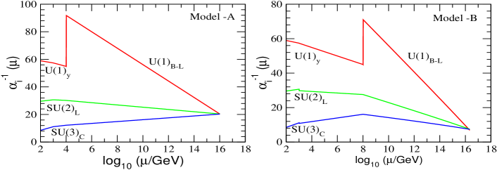
Figure 1: The evolution of the gauge couplings in models with additional light multiplets. The left- (right-) panel corresponds to Model A (Model B).

Model	${\rm M_{R}}$	${\rm M_{U}}$	${\alpha_{G}^{-1}}$
	(GeV)	(GeV)
	$10^{9}$	$1.15\times 10^{16}$	22.22
A	$10^{5}$	$1.10\times 10^{16}$	20.83
	$10^{4}$	$10^{16}$	20.40
	$10^{9}$	$1.82\times 10^{16}$	7.58
B	$10^{8}$	$2.00\times 10^{16}$	10.13

Table 4: Sample solutions for low intermediate scales, $M_{R}$, in two models with additional light multiplets at the intermediate scale (see text).

We show in the next section that the intermediate scale in the triplet model has a lower bound at $10^{9}$ GeV which is expected to be increased by additional Higgs scalars at the $M_{R}$ scale.

From the above two examples and earlier investigations it is clear that right-handed mass scales as low as $M_{R}=5$ TeV $-10^{10}$ GeV are viable when additional light chiral multiplets at the $M_{R}$ scale are admitted. As already noted, such low scales are necessary for the successful implementation of leptogenesis in the doublet model (Model I). Obviously, these models may have interesting new signatures at LHC and future collider experiments. It is noteworthy that all the light multiplets exploited in the two models are contained in $SO(10)$ representations which have been invoked in the literature anyway for various purposes.

IV Lower bound on intermediate scale in the triplet model

As pointed out earlier, the high dimensional Higgs representations like ${\bf{210}}$ and/or ${\bf{126}+\overline{126}}$ result in large threshold corrections at the GUT scale even if their superheavy components are only few times heavier or lighter than $M_{U}$. In this respect, threshold corrections in the triplet model with ${\bf{126}+\overline{126}}$ are more significant compared to those in the doublet model which uses ${\bf{16}+\overline{16}}$. Normally, one would therefore expect to obtain lower $M_{R}$ in the former model.

In this section we show that this is not true and, in fact, establish that $M_{R}$ cannot be lower than $10^{9}$ GeV in the triplet model. This lower bound is set by the perturbative renormalization group constraint when parity survives in the left-right gauge group as happens in the case of $\cal{G}_{LR}$. As the GUT threshold effects contribute only at the unification scale, we use the two-loop equation for $\alpha_{BL}$ between $M_{R}$ and $M_{U}$ with the corresponding coefficients given in eq. (21) and eq. (48). It is seen that if $M_{R}\leq 10^{9}$ GeV, $\alpha_{BL}$ exceeds the perturbative limit ($\simeq 1$) before the GUT scale is reached.

Analytically, this behavior of the gauge coupling becomes transparent by noting that the position of the Landau pole ($\mu_{0}$), where $g_{BL}(\mu_{0})=\infty$, is given by,

$$\mu_{0} = M_{R}~{}\exp\left[{2\pi\over a^{\prime}_{BL}}{1\over\alpha_{BL}(M_{R})}\right].$$ (133)

Here

$${1\over\alpha_{BL}(M_{R})}={5\over 2}\left({1\over\alpha_{Y}(M_{Z})}-\Theta_{Y}+\Delta_{Y}\right)~{}~{}~{}~{}~{}~{}~{}~{}~{}~{}~{}~{}~{}~{}~{}~{}~{}~{}~{}~{}~{}~{}~{}$$

$$-{3\over 2}\left({1\over\alpha_{2L}(M_{Z})}-\Theta_{2L}+\Delta_{2L}\right)-{1\over 4\pi}\left(5a_{Y}-3a_{2L}\right)\ln{M_{R}\over M_{Z}}.$$

(134)

Using eq. (134) we calculate $\alpha_{BL}^{-1}(M_{R})$ for $M_{R}=10^{3}$ GeV to $10^{11}$ GeV from low energy data ignoring the small threshold effect due to superpartners and use them in eq. (133) to estimate the value of $\mu_{0}$. Our two-loop estimations of the pole position are shown in Table 5 for the triplet model with $a^{\prime}_{BL}=24$. The two-loop corrections predict slightly lower values of $\mu_{0}$ than eq. (133). For intermediate scales $M_{R}=1$ TeV to $10^{9}$ GeV, the pole positions are found in the range $7.76\times 10^{13}$ GeV to $1.44\times 10^{16}$ GeV indicating that for the $U(1)_{BL}$ gauge coupling perturbation theory breaks down below the GUT scale for these values of $M_{R}$. When $M_{R}\mathop{\smash{>}}\limits_{\sim}10^{10}$ GeV, the pole positions occur clearly above the GUT scale with $\mu_{0}\mathop{\smash{>}}\limits_{\sim}3.46\times 10^{16}$ GeV. In other words, with only the minimal particle content needed to maintain supersymmetry and left-right symmetry below the GUT scale, from the requirement of perturbativity the triplet model leads to the conservative lower bond on the intermediate scale,

$$M_{R}>10^{9}~{}{\rm GeV}.$$ (135)

Inclusion of additional new scalar degrees of freedom anywhere between $M_{R}$ to $M_{U}$ would increase the one-loop beta-function coefficient of the $U(1)_{B-L}$ gauge coupling and bring down the pole position further. This, in turn, would further tighten the lower bound on $M_{R}$ beyond $10^{9}$ GeV. This is why, unlike in the doublet model, the presence of additional light scalars near $M_{R}$ cannot reduce the value of the intermediate scale in the triplet model.

In contrast to the triplet model for which $a^{\prime}_{BL}=24$, the doublet model has $a^{\prime}_{BL}=9$ which enhances the argument of the exponential on the RHS of eq. (133) by a factor $\simeq 24/9=2.66$ compared to the triplet model for the same value of $M_{R}$. Such a factor in the argument pushes the Landau pole to a position much above the GUT scale. Thus, even with $M_{R}=1$ TeV, whereas the triplet model pole position is at $\mu_{0}\simeq 1.18\times 10^{14}$ GeV which is approximately two orders below the GUT scale, in the the doublet model the pole occurs at $\mu_{0}\simeq 3.3\times 10^{32}$ GeV. Although this latter scale for the doublet model is expected to be substantially lower because of the contribution of superheavy particles near the GUT scale, it is clear that the coupling constant never hits a Landau pole below the GUT-Planck scales $\simeq 10^{18}$ GeV. This tallies with the results in Sec.III where solutions have been obtained using threshold and gravitational corrections.

$M_{R}$	${1\over\alpha_{BL}(M_{R})}$	$\mu_{0}$
(GeV)		(GeV)
$10^{3}$	$97.429$	$7.76\times 10^{13}$
$10^{5}$	$86.407$	$4.56\times 10^{14}$
$10^{7}$	$75.406$	$2.56\times 10^{15}$
$10^{8}$	$69.907$	$6.16\times 10^{15}$
$10^{9}$	$64.409$	$1.44\times 10^{16}$
$10^{10}$	$58.912$	$3.46\times 10^{16}$
$10^{11}$	$53.415$	$8.31\times 10^{16}$

Table 5: Location of Landau poles, $\mu_{0}$, signifying violation of perturbativity, for different choices of the intermediate scale $M_{R}$ in the triplet model.

With such a lower bound on $M_{R}$ in the triplet model, this version of SUSY $SO(10)$ rightly deserves its description as a high scale theory. The SUSY $SO(10)$ triplet model appears to fit ideally for description of quark-lepton masses and mixings through high-scale $b-\tau$ unification and type II see-saw dominance or even through type I see-saw mechanism min2 ; goh ; babu .

Since $M_{R}\mathop{\smash{>}}\limits_{\sim}10^{9}$ GeV in the triplet model, the lightest right-handed neutrino mass could satisfy the gravitino constraint, but in this case generating the quark and lepton masses and mixings has to be re-examined. While a detailed analysis of neutrino data is yet to emerge in the doublet model, it is well known that reproducing small neutrino masses is no problem even if the right-handed neutrinos are near the TeV scale. With such a low value of $M_{R}$ the desired criteria of TeV scale resonant leptogenesis is fulfilled and through the $W_{R}^{\pm}$ and $Z_{R}$ bosons and the light Higgs scalars, $\chi_{L}^{\pm},\chi_{L}^{0}$, $\chi_{R}^{\pm}$, and $\chi_{R}^{0}$, the model can be tested at the LHC and ILC. The superpartner of the lightest right-handed neutrino in the doublet model may also be a good candidate for dark matter.

V Remarks on light scalars and fermion masses in minimal $SO(10)$

One of the most appealing features of the minimal supersymmetric $SO(10)$ model is that one can calculate the pattern of symmetry breaking and predict fermion mass relations at the GUT scale fmsen . Concomitant with these, in the minimal model, is an intermediate left-right breaking scale, $M_{R}$, constrained to be rather close to the GUT scale $M_{U}$. Can the virtues of the model be made to survive when $M_{R}$ is lowered?

Let us briefly summarize the salient features with reference to Model II. The Higgs fields are:

$$\Phi\equiv{\bf 210},~{}~{}~{}~{}~{}\Sigma\equiv{\bf 126},~{}~{}~{}~{}~{}\bar{\Sigma}\equiv{\bf\overline{126}},~{}~{}~{}~{}~{}H\equiv{\bf 10},$$

where $\Delta_{L,R}\subset\Sigma$ and $\phi\subset H$. The fermions belong to the representation $\Psi\equiv$ 16. The complete superpotential of the model can then be written as

$$W=W_{Y}+W_{H},$$ (136)

where the Yukawa couplings are in $W_{Y}$ and the scalar potential can be derived from $W_{H}$. They can be written as (we follow the notations of ref. min3 )

$$W_{Y} = Y_{10}\Psi\Psi H+Y_{126}\Psi\Psi\bar{\Sigma},$$

$$W_{H} = {m_{\Phi}\over 4!}\Phi\Phi+{\lambda\over 4!}\Phi\Phi\Phi+{M\over 5!}\Sigma\bar{\Sigma}+{\eta\over 4!}\Phi\Sigma\bar{\Sigma}$$ (137)

$$+m_{H}HH+{1\over 4!}\Phi H~{}(\alpha\Sigma+\beta\bar{\Sigma}).$$

As usual, minimization of the scalar potential gives the allowed values of the $vev$ of the different fields. In addition, fermion mass relations are also determined in terms of the parameters of the model.

It may appear that the solutions presented earlier with lowered left-right symmetry breaking scales are in conflict with results on fermion masses. However, this need not be the case. For example, when gravitational corrections are included, there may well be non-renormalizable terms in the superpotential, suppressed by the Planck scale, which can contribute to the Yukawa couplings after the GUT symmetry breaking by the field $\Phi$. Thus, in the presence of such corrections, the superpotential will have to be supplemented by

$$W_{Y}^{G}={1\over M_{Pl}}(Y^{G}_{10}\Psi\Psi H\Phi+Y^{G}_{126}\Psi\Psi\bar{\Sigma}\Phi)+\cdots.$$ (138)

These new interactions will be suppressed by ${\langle\Phi\rangle/M_{Pl}}$. But $\langle\Phi\rangle\sim M_{U}$ is close to the Planck scale, as we have illustrated, and hence the suppression need not be too much. In addition, the non-renormalizable couplings $Y^{G}$ could also be large. Then the fermion mass relations obtained for the minimal supersymmetric $SO(10)$ models could be radically affected. Fermion mass relations can also get changed in the presence of new Higgs scalars. Thus the low intermediate mass scales, $M_{R}$, obtained in the present analysis need not be inconsistent with the fermion mass relations.

At the tree level, the minimal triplet model predicts  min3 masses near $M_{R}$ for additional states belonging to ${\bf 210}$ with the quantum numbers

$$E_{L}(3,3,1,4/3)\oplus{\overline{E}}_{L}(\overline{3},3,1,-4/3),$$

$$E_{R}(3,1,3,4/3)\oplus{\overline{E}}_{R}(\overline{3},1,3,-4/3).$$ (139)

We have checked that with the minimal Higgs content, the renormalizable doublet model also leads to similar light Higgs scalars. It has been further noted in ref. min3 that these states prevent having parity conserving ${\cal G}_{LR}$ at any value of the intermediate scale below $M_{U}$. We remark that their presence at $M_{R}$ sufficiently lower than $M_{U}$, apart from being in conflict with $\sin^{2}\theta_{W}(M_{Z})$ and $\alpha_{S}(M_{Z})$, spoils perturbative gauge coupling evolutions by developing Landau poles in the coupling constants in the region $M_{R}<\mu<M_{U}$. This difficulty could be avoided f6 by extensions of the minimal doublet or the triplet model through the inclusion of non-renormalizable operators and/or additional $SO(10)$ Higgs representations, like $\bf{54}$. For example, the presence of the non-renormalizable term in the superpotential

$$W_{gr} = {\lambda^{G}\over{4!M_{G}}}\Phi^{4},$$

with $M_{G}=M_{Pl}$, or (string) compactification scale, can lift the masses of these light scalars close to the GUT scale when the ${\bf 210}$ gets $vev$ along the direction $\langle\Phi^{0}\{15,1,1\}\rangle~{}\sim~{}M_{U}$, leading to $M_{E}={{2\lambda^{G}m_{\Phi}^{2}}/{\lambda^{2}{M_{G}}}}$. Then their contributions are added to GUT-threshold effects, as discussed earlier.

VI Summary and conclusion

In this work, we have discussed the question of low intermediate left-right symmetry breaking scales, as preferred by leptogenesis, in the minimal supersymmetric $SO(10)$ GUTs with only doublet Higgs scalars as well as with triplet scalars. In view of the presence of additional scalar components predicted from mass spectra analysis min3 which disrupt perturbativity and gauge coupling unification, the minimal renormalizable triplet model with Higgs representations ${\bf 210\oplus 126\oplus{\overline{126}}\oplus 10}$ is ruled out as a candidate for any value of left-right symmetry breaking intermediate scale. With the added presence of a Higgs representation $54$ and/or non-renormalizable interactions, these unwanted scalar components are made superheavy and we find, in agreement with previous work, that in the minimal models, at the one-loop level gauge coupling unification requires the scale of left-right symmetry breaking to be close to the GUT scale f7 . Inclusion of the two-loop contributions eliminates even this possibility as no solution can be found at all with an intermediate scale. On the other hand, evading the gravitino problem, which would otherwise plague successful big bang nucleosynthesis, would require $M_{R}\leq 10^{9}~{}{\rm GeV}$. We have pointed out that this impasse can be circumvented in the case of the doublet model by including threshold corrections near the GUT scale, including non-renormalizable interactions due to gravity induced Planck scale effects, or by adding new light scalar multiplets. In the last alternative, the additional light submultiplets used are present in representations commonly used in $SO(10)$ non-minimal models, but they are different from those which emerge from mass spectra analysis min3 . These considerations allow the left-right symmetry breaking scale to be low, as low as even a few TeV, making it phenomenologically interesting. The unification scale obtained in the doublet model using the first two methods turns out to be large, making it safe for Higgsino mediated proton decay as well as with fermion mass relations. In the triplet model, although threshold effects can easily decrease the intermediate scale, we find a perturbative lower bound, $M_{R}>10^{9}$ GeV, below which the intermediate scale cannot be lowered. With this bound, the triplet model with an added ${54}$ and/or nonrenormalizable interactions emerges as a high scale theory of SUSY $SO(10)$ description of fermion masses and mixings. In this model the possibility of meeting the gravitino constraint can be fulfilled provided neutrino masses and mixings are successfully reproduced with $M_{R}\mathop{\smash{>}}\limits_{\sim}10^{9}$ GeV. With $M_{R}$ in the TeV region in the doublet model, apart from successful resonant leptogenesis with full compliance of the gravitino constraint, the model predictions can be tested through their various manifestations at the LHC and ILC.
                                                            ACKNOWLEDGMENTS
M. K. P. thanks Harish-Chandra Research Institute, Allahabad, India for hospitality and Institute of Physics, Bhubaneswar, India for facilities.

References

• (1) J. C. Pati and A. Salam, Phys. Rev. D10 (1974) 275; R. N. Mohapatra and J. C. Pati, Phys. Rev. D11 (1975) 566; R. N. Mohapatra and J. C. Pati, Phys. Rev. D11 (1975) 2558; G. SenjanoviΔ‡ and R. N. Mohapatra, Phys. Rev. D12 (1975) 1502.
• (2) D. Chang, R. N. Mohapatra and M. K. Parida, Phys. Rev. Lett. 52 (1984) 1072; Phys. Rev. D30 (1984) 1052; D. Chang, R. N. Mohapatra, J. M. Gipson, R. E. Marshak and M. K. Parida, Phys. Rev. D31 (1985) 1718.
• (3) H. Georgi, in Particles and Fields – 1974, ed. C. A. Carlson (AIP, New York, 1975); H. Fritzsch and P. Minkowski, Ann. Phys. (N.Y.) 93 (1975) 193; T. Clark, T. Kuo and N. Nakagawa, Phys. Lett. B115 (1982) 26; C. S. Aulakh and R. N. Mohapatra, Phys. Rev. D28 (1983) 217.
• (4) K. S. Babu and R. N. Mohapatra, Phys. Rev. Lett. 70 (1993) 2845.
• (5) B. Bajc, G. SenjanoviΔ‡ and F. Vissani, Phys. Rev. Lett. 90 (2003) 051802; H. S. Goh, R. N. Mohapatra and S. P. Ng, Phys. Lett. B570 (2003) 215; Phys. Rev. D68 (2003) 115008; S. Bertolini, M. Frigerio and M. Malinsky, Phys. Rev. D70 (2004) 095002.
• (6) B. Bajc, A. Melfo, G. SenjanoviΔ‡ and F. Vissani, Phys. Rev. D70 (2004) 035007; C. S. Aulakh, B. Bajc, A. Melfo, G. SenjanoviΔ‡, and F. Vissani, Phys. Lett. B588 (2004) 196; T. Fukuyama, A. Ilakovic, T. Kikuchi, S. Meljanac and N. Okada, J. Math. Phys. 46 (2005) 033505; Eur. Phys. J. C42 (2005) 191.
• (7) S. M. Barr, Phys. Rev. Lett. 92 (2004) 101601; U. Sarkar, Phys. Lett. B622 (2005) 118; K. S. Babu, I. Gogoladze, P. Nath, and R. M. Syed, Phys. Rev. D72 (2005) 095011.
• (8) S. Davidson and A. Ibarra, Phys. Lett. B535 (2002) 25: T. Hambye and G. SenjanoviΔ‡, Phys. Lett. B582 (2004) 73; G. D’Ambrosio, T. Hambye, A. Hektor, M. Raidal and A. Rossi, Phys. Lett. B604 (2004) 199; L. Boubekeur, T. Hambye and G. SenjanoviΔ‡, Phys. Rev. Lett. 93 (2004) 111601; N. Sahu and S. Uma Sankar, Phys. Rev. D71 (2005) 013006.
• (9) M. Flanz, E. A. Paschos, and U. Sarkar, Phys. Lett. B345 (1995) 248; Phys. Lett. B389 (1996) 69; A. Pilaftsis, Nucl. Phys. B692 (2004) 303; W. Buchmuller and M. Plumacher, Phys. Lett. B431 (1998) 354; W. Buchmuller, P. Di Bari, and M. Plumacher, New J. Phys. 6 (2004) 105.
• (10) Electric charge is normalized in terms of the $SU(2)_{L}$, $SU(2)_{R}$, $U(1)_{(B-L)}$ and $U(1)_{Y}$ quantum numbers as $Q=T_{3L}+T_{3R}+{B-L\over 2}=T_{3L}+{Y\over 2}$.
• (11) H. Georgi and C. Jarlskog, Phys. Lett. B86 (1979) 297.
• (12) R. N. Mohapatra, Phys. Rev. Lett. 56 (1986) 561; R. N. Mohapatra and J. W. F. Valle, Phys. Rev. D34 (1986) 1642.
• (13) U. Sarkar, ref.min4 .
• (14) P. Minkowski, Phys. Lett. B67 (1977) 421; M. Gell-Mann, P. Ramond and R. Slansky, in Supergravity, eds. D. Freedman et al. (North-Holland, Amsterdam, 1980); T. Yanagida, in proc. KEK workshop, 1979 (unpublished); R. N. Mohapatra and G. SenjanoviΔ‡, Phys. Rev. Lett. 44 (1980) 912; S. L. Glashow, CargΓ¨se lectures, (1979).
• (15) H. S. Goh, R. N. Mohapatra and S. Nasri, Phys. Rev. D70 (2004) 075022; K. S. Babu and C. Macesanu, Phys. Rev. D72 (2005) 115003.
• (16) Here, for simplicity of discussion, we have considered $\tilde{f}$ to be multiplying a unit matrix in flavor space. The RH neutrino masses can also be lowered through small eigenvalues, if $\tilde{f}$ has a non-trivial matrix structure ji .
• (17) M. Y. Khlopov and A. D. Linde, Phys. Lett. B138 (1984) 265; J. R. Ellis, D. V. Nanopoulos and S. Sarkar, Nucl. Phys. B259 (1985) 175; J. R. Ellis, D. V. Nanopoulos, K. A. Olive and S. J. Rey, Astropart. Phys. 4 (1996) 371; M. Kawasaki and T. Moroi, Prog. Theor. Phys. 93 (1995) 879; V. S. Rychkov and A. Strumia, hep-ph/0701104.
• (18) The small logarithmic running between the electroweak scale and the SUSY scale ($M_{S}$) and, in effect, set $M_{S}$ and $M_{Z}$ to be the same.
• (19) M. Carena, S. Pokorski and C. E. M. Wagner, Nucl. Phys. B406 (1993) 59.
• (20) H. Baer, J. Ferrandis, S. Kraml and W. Porod, Phys. Rev. D73 (2006) 015010.
• (21) P. Langacker and N. Polonsky, Phys. Rev. D47 (1993) 4028.
• (22) M. K. Parida, B. Purkayastha, C. R. Das and B. D. Cajee, Eur. Phys. J C28 (2002) 353; M. K. Parida and B. D. Cajee, Eur. Phys. J C44 (2005) 447.
• (23) Q. Shafi and C. Wetterich, Phys. Rev. Lett. 52 (1984) 875; C. T. Hill, Phys. Lett. B135 (1984) 47; L. Hall and U. Sarid, Phys. Rev. Lett. 70 (1993) 2673.
• (24) M. K. Parida and P. K. Patra, Phys. Rev. D39 (1989) 2000; M. K. Parida and P. K. Patra, Phys. Lett. B432 (1990) 45.
• (25) Here, $M_{S}=M_{Z}$ has been assumed. If $M_{S}$ is set at 1 TeV, then one finds $M_{R}^{0}=5.0\times 10^{15}(1.6\times 10^{15})$ GeV and $M_{U}^{0}=1.9\times 10^{16}(6.2\times 10^{15})$ GeV, at the one-loop level in Model I (Model II).
• (26) X. Ji, Y. Li, R. N. Mohapatra and S. Nasri, hep-ph/0605088; J. C. Pati, Phys Rev. D68 (2003) 072002.
• (27) S. M. Barr, ref.min4 , C. H. Albright and S. M. Barr, Phys. Rev. D69 (2004) 101601; K. L. McDonald, B. H. J. McKellar and A. Mastrano, Phys.Rev. D70 (2004) 053012; D. G. Lee and R. N. Mohapatra, ref.lee .
• (28) S. Weinberg, Phys. Lett. B91 (1980) 51.
• (29) L. Hall, Nucl. Phys. B178 (1981) 75; M. Shifman, Int. J. Mod. Phys. A11 (1996) 5761.
• (30) B. Ovrut and H. Schnitzer, B179 (1981) 381; W. J. Marciano, in Field Theory in Elementary Particles, ed. A. Perlmutter (Plenum, New York 1982), Proceedings of Orbis Scientiae Vol. 19; in Fifth Workshop on Grand Unification. Philadelphia, Pennsylvania, 1983, eds. H. A. Weldon, P. Langacker and P. J. Steinhardt (Birkhauser, Boston, 1983); R. N. Mohapatra and M. K. Parida, Phys. Rev. D47 (1993) 264.
• (31) One must also ensure that the ratios ${M_{i}\over M_{U}},i=1,2,3$ lie within an appropriate range, say 0.1 to 10, and ought not exceed the Planck mass.
• (32) D. Costa, P. Perez and R. Felipe, arXiv: hep-ph/0610178.
• (33) D. G. Lee and R. N. Mohapatra, Phys. Rev. D52 (1995) 4125; M. Bando, J. Sato and T. Takahashi, Phys. Rev. D52 (1995) 3076; E. Ma, Phys. Rev. D51 (1995) 236; E. Ma, Phys. Lett. B344 (1995) 164.
• (34) K. S. Babu and S. M. Barr, Phys. Rev. D48 (1993) 5354; B. Dutta, Y. Mimura and R. N. Mohapatra, Phys. Rev. Lett. 94 (2005) 091804; Phys. Rev. D72 (2005) 075009.
• (35) B. Bajc, A. Melfo, G. SenjanoviΔ‡ and F. Vissani, Phys. Rev. D73 (2006) 055001; Phys. Lett. B634 (2006) 272.
• (36) These states represent pseudo-Goldstone bosons and may also acquire masses near the $M_{U}$ scale through loops.
• (37) Here it has been assumed that the light scalar components in $\{15,3,1\}\oplus\{15,1,3\}\subset{\bf 210}$, emerging from mass spectra predictions, are made superheavy. This is possible if, for example, the minimal models are extended by the addition of a Higgs representation $\bf{54}$ in each case. But the situation would be worse still in both the models if the scalar components remain light in the absence of ${\bf 54}$ or suitable nonrenormalizable terms in the superpotential.