Chromomagnetic Dipole Moment of the Top Quark Revisited

Abstract

We study the complete one-loop contributions to the chromagnetic dipole moment $\Delta\kappa$ of the top quark in the Standard Model, two Higgs doublet models, topcolor assited technicolor models (TC2), 331 models and extended models with a single extra dimension. We find that the SM predicts $\Delta\kappa=-0.056$ and the predictions of the other models are also consitent with the constraints imposed on $\Delta\kappa$ by low-energy precision measurements.

I Introduction

The fact that the top quark mass $\sim 172GeV$ uno is of the same order of magnitude then the electroweak symmetry breaking (EWSB) scale $\nu=(\sqrt{2}G_{F})^{-1/2}=246$ GeV suggests that the top quark may be more sensitive to new physics effects than the remaining ligthter fermions. With the advent of the CERN Large Hadron Collider (LHC), 8 millions top-quark pairs will be produced per year with an integrated luminosity of $10fb^{-1}$ dos . This number will increase by one oder of magnitude with the high luminosity option $(100fb^{-1})$. Therefore, the properties of the top quark will be examined with significant precision at the LHC. In particular, the interest in non-standard $ttg$ couplings arised some time ago when it was realized that the presence of non-Standard-Model couplings could lead to significant modifications in the total and differential cross sections of top-pair production at hadron colliders tres ; cuatro . If the source of this new physics is at the TeV scale, it has been pointed out tres that the leading effect may be parametrized by a chromomagnetic dipole moment (CMDM) $\Delta\kappa$ of the top quark since this is the lowest dimension CP-conserving operator arising from an effective Lagrangian contributing to the gluon-top-quark coupling,

$${\cal L}_{5}=(\Delta\kappa/2)(g_{s}/4m_{t})\bar{u}(t)\sigma_{\mu\nu}F^{\mu\nu,\alpha}T^{\alpha}u(t)$$ (1)

where $g_{s}$ and $T^{\alpha}$ are the $SU(3)_{c}$ coupling and generators, respectively. $F^{\mu\nu,\alpha}=\partial^{\mu}A^{\nu,\alpha}-\partial^{\nu}A^{\mu,\alpha}-g_{s}f^{\alpha\beta\gamma}A^{\mu,\beta}A^{\nu,\gamma}$ is the gluonic antisymmetric tensor.

The effects due to $\Delta\kappa\neq 0$ have been examined in flavor physics as well as in topquark cross section measurements tres ; cuatro ; cinco . In the latter case, the parton level differential cross sections of $gg\to\bar{t}t$ and $\bar{q}q\to\bar{t}t$ (the dominant channel at Fermilab Tevatron energies) were calculated tres ; cuatro ; seis . The combined effects of the chromomagnetic and the chromoelectric dipole moment of the top quark on the reaction $p\bar{p}\to t\bar{t}X$ were investigated in Ref. cinco . Moreover, previous analysis has revealed the the differential cross section is sensitive to the sign of the anomalous chromomagnetic dipole moment on account of the interference with the SM coupling. This can lead to a significant suppression or enhancement in the production rate tres .

Cross section measurements at the Tevatron are expected to constrain the CMDM of the top quark to $|\Delta\kappa|\leq 0.15-0.20$ siete . Since the influence of $\Delta\kappa$ grows rapidly with the increasing center of mass energy, this bound will be improved by one order of magnitude at the LHC with a luminosity of $100fb^{-1}$ ocho . On the other hand, it has been pointed out nueve that the CLEO data on $b\to s\gamma$ gives already a constraint as strong as that expected at the LHC, $-0.03\leq\Delta\kappa\leq 0.01$. Low-energy precision measurements have produced similar constraints for the non-standard top-quark couplings $tbW,ttZ,tcV,tcH$, with $V=\gamma,g,Z$ diez ; once . It is interesting to notice that the CP violating chromoelectric dipole moment of the top quark, which is much further suppressed than the CMDM, has not been constrained yet by low-energy precision measurements. However, the CP-odd observables induced by a chromoelectric dipole moment for the $t\bar{t}$ system have been studied in $p-p$ and $p-\bar{p}$ collisions doce .

In the Standard Model (SM) trece , $\Delta\kappa$ arises at the one-loop level and it is of order $10^{-2}$ for a light Higgs boson mass nueve . A large value for $\Delta\kappa$ arises naturally in dynamical electroweak-symmetric breaking models such as technicolor or topcolor tres . In two Higgs doublet models (THDM) and for QCD-SUSY corrections, previous studies have found that $\Delta\kappa$ could be as large as $10^{-1}$ nueve . The search for $\Delta\kappa$ effects induced in the LHC/ILC accelerators constitute then a window to look for physics beyond the SM.

Motivated by the fact that there is no detailed study in the literature of the top-quark CMDM $\Delta\kappa$, in the present paper we make a critical reanalysis of the one-loop contributions to $\Delta\kappa$ in the SM, the two-Higgs doublet model (THDM-II), topcolor assited technicolor (TC2) models, as well as in the so called 331 models and in the framework of a universal extra dimension with the SM fields propagating in the bulk. We have found that the predictions of all these models are consistent with the constraints obtained from low-energy precision measurements nueve .

The paper is organized as follows. In Section II we present the general framework required in each model in order to compute the respective one-loop contributions to the top-quark CMDM. In this paper we put together the results obtained for the top-quark CMDM in each one of the models addressed in this paper. The concluding remarks are included in section III and in the Appendix we present the analytical expressions obtained in our calculation for the one-loop Feynman diagrams contributing to the CMDM.

II Framework

In this section, we present the basic elements of the models in which we have computed the top-quark CMDM.

II.1 Standard Model

In the SM diez the top-quark CMDM arises from loops containing the electroweak bosons $W^{\pm},Z,h^{0}$ with their respective would-be Goldstone bosons $G^{\pm}_{W}$ and $G_{Z}$, or just gluons nueve . Figures 1 and 2 show the generic diagrams for the electroweak contributions to the CMDM. In Table I we include the respective Feynman rules used to compute these contributions. The diagrams shown in Figs. 1b and 2b induce the QCD contribution to the CMDM of the top quark. Notice that the contribution arising from diagram $2b$ was not considered in our previous work on $\triangle\kappa$ nueve .

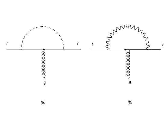
Figure 1: Feynman diagrams that contribute to the CMDM

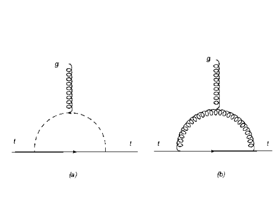
Figure 2: Feynman diagrams for the QCD contributions to the CMDM

	$A$	$B$	$A^{{}^{\prime}}$	$B^{{}^{\prime}}$
$tth^{0}$	$-i\frac{gmt}{2M_{W}}$	$-i\frac{gmt}{2M_{W}}$	$-i\frac{gmt}{2M_{W}}$	$-i\frac{gmt}{2M_{W}}$
$ttG_{Z}$	$\frac{gmt}{2M_{W}}$	$-\frac{gmt}{2M_{W}}$	$\frac{gmt}{2M_{W}}$	$-\frac{gmt}{2M_{W}}$
$ttG_{W}$	0	$i\frac{gmt}{2M_{W}}$	$i\frac{gmt}{2M_{W}}$	0
$tbW_{\mu}$	$-i\frac{g}{\sqrt{2}}$	0	$-i\frac{g}{\sqrt{2}}$	0
$ttZ_{\mu}$	$-i\frac{g}{c_{W}}(\frac{1}{2}-\frac{2}{3}s_{W}^{2})$	$i\frac{g}{c_{W}}\frac{2}{3}s_{W}^{2}$	$-i\frac{g}{c_{W}}(\frac{1}{2}-\frac{2}{3}s_{W}^{2})$	$i\frac{g}{c_{W}}\frac{2}{3}s_{W}^{2}$

Table 1: Feynman rules for the SM contributions to the CMDMT

The contributions obtained for each SM QCD and electroweak one-loop diagrams for the CMDM are given by

$$\Delta\kappa_{(\mu)}^{QCD} = -6.4\times 10^{-2}$$

$$\Delta\kappa_{(s)}^{h^{0}} = 8.7\times 10^{-3}\;\;\;\;,\;\;\;m_{h}=120GeV$$

$$\Delta\kappa_{(s)}^{G_{Z}} = -5.1\times 10^{-3}$$

$$\Delta\kappa_{(s)}^{G_{W}} = -5.2\times 10^{-3}$$

$$\Delta\kappa_{(\mu)}^{W} = 9.9\times 10^{-3}$$

$$\Delta\kappa_{(\mu)}^{Z} = -7.5\times 10^{-4}$$

where the subindices $(\mu)$ or $(s)$ mean that the internal boson line in the one loop diagram corresponds to gauge or scalar bosons, respectively. Taking the sum of only the electroweak contributions, we get

$$\Delta\kappa^{EW}=7.5\times 10^{-3}$$ (3)

which is about $12\%$ of the QCD contribution but with opposite sign. The SM prediction for the top-quark CMDM is thus given by

$$\Delta\kappa^{SM}=-5.6\times 10^{-2}$$ (4)

II.2 THDM-II

The Yukawa couplings needed to compute the top-quark CMDM in the two Higgs doublet model (THDM-II) are given by the Lagrangian

$$-{\cal L}_{Y}=h_{t}\overline{Q}_{L}\widetilde{\phi}_{1}t_{R}+h_{b}\overline{Q}_{L}\phi_{2}b_{R}+h.c.$$ (5)

where we have used a discrete symmetry $\phi_{1}\to\phi_{1}\to\phi_{2}\to-\phi_{2}$ to avoid flavor-changing neutral couplings for the quarks at the tree level catorce . $Q_{L}$ corresponds to the quark doublet for the third family. After the spontaneous symmetry breaking, with $\nu_{1}$ and $\nu_{2}$ the respective vacuum expectation values for the two Higgs doublets and $\tan\beta=\nu_{1}/\nu_{2}$, there are two physical charged scalar bosons $H^{\pm}$ and three physical neutral scalar bosons $h,H$ and $A$, and the respective would-be Goldstone bosons $G^{\pm}_{W}$ and $G_{Z}$. The Feynman rules required to compute the top-quark CMDM in this model are depicted in Table II. We have neglected the $H^{\pm}tb$ coupling which is proportional to the bottom quark mass. The $\cos\theta$ is the mixing angle of the two CP-even scalar fields, $h,H$.

The one-loop effects induced by the THDM on the CMDM were also calculated in Ref.[9]. However, the results obtained in this case were used only to get constraints on the THDM parameters involved in the calculation by requiring in turn that these contributions also agreed with the low-energy constraints on the CMDM nueve .

	$A$	$B$	$A^{{}^{\prime}}$	$B^{{}^{\prime}}$
$tth$	$-i\frac{gm_{t}c_{\theta}}{2M_{W}s_{\beta}}$	$-i\frac{gm_{t}c_{\theta}}{2M_{W}s_{\beta}}$	$-i\frac{gm_{t}c_{\theta}}{2M_{W}s_{\beta}}$	$-i\frac{gm_{t}c_{\theta}}{2M_{W}s_{\beta}}$
$ttA^{0}$	$\frac{gm_{t}}{2M_{W}t_{\beta}}$	$-\frac{gm_{t}}{2M_{W}t_{\beta}}$	$\frac{gm_{t}}{2M_{W}t_{\beta}}$	$-\frac{gm_{t}}{2M_{W}t_{\beta}}$
$tbH$	$0$	$i\frac{gm_{t}}{\sqrt{2}M_{W}t_{\beta}}$	$i\frac{gm_{t}}{\sqrt{2}M_{W}t_{\beta}}$	0

Table 2: Feynman rules for the THDM contributions to the CMDMT

In the THDM-II, the charged Higgs boson $H^{+}$ and the neutral Higgs bosons $h^{0},H^{0},A^{0}$ give the following contributions to the CMDM,

$$\Delta\kappa^{H^{+}}_{(s)} = 3.7\times 10^{-3},\;\;1.4\times 10^{-3},\;\;6.2\times 10^{-4}\;\;,$$

$$\Delta\kappa^{A^{0}}_{(s)} = -3.6\times 10^{-3},\;\;-2.8\times 10^{-3},\;\;-1.8\times 10^{-3},$$

$$\Delta\kappa^{h^{0}}_{(s)} = 8.6\times 10^{-3},$$

$$\Delta\kappa^{H^{0}}_{(s)} = 4.3\times 10^{-3},\;\;$$ (6)

where we have taken $\tan\beta=1$, $\sin\theta=1/\sqrt{2}$ and $m_{H^{+}}/m_{A^{0}}=250,350,500$ GeV. The masses for the CP-even scalar Higgs $h^{0},H^{0}$ are $120,300$ GeV, respectively. We observe that these contributions become smaller with heavier scalars, which agrees with the expectations given by the decoupling theorem. Taking into account the contribution of the $H^{+},H^{0},A^{0}$ fields, we get for the scalar contributions of the THDM-II to the CMDM the result

$$\Delta\kappa^{THDM}_{(s)}=4.4\times 10^{-3},\;\;3.0\times 10^{-3},\;\;3.1\times 10^{-3}.$$ (7)

Then, the THDM contribution to the CMDM is one order of magnitude smaller than the SM value.

When $\tan\beta=10$ the predicted value for $\Delta\kappa$ due to the CP-even neutral scalar is of the same order of magnitude than for $\tan\beta=1$, but the CP-odd scalar contribution is two orders of magnitude lower, and the charged scalar Higgs is one order of magnitude lower than the value given by $\tan\beta=1$. In this case the most important contribution is coming from the $H^{0}$ scalar field, and the $\Delta\kappa^{THDM}$ practically does not change for this value of $\tan\beta$. However, for a bigger value of this parameter $\tan\beta=100$, the term proportional to the bottom quark mass in the $tbH^{+}$ vertex is more important than the coupling proportional to the top quark mass. The contributions coming from the CP-even Higgs fields are unchanged and the CP-even neutral scalar is very much supppresed, but the charged Higgs is incresed in one order of magnitude, i.e., for $m_{H^{+}}=250$ GeV the CMDM is of the order of $3\times 10^{-2}$ which is as big as the SM value but with opposite sign.

II.3 The 331 model

In the so-called 331 models, which are based on the $SU(3)_{c}\otimes SU(3)_{L}\otimes U(1)$ gauge group quince ; dieciseis , the cancellation of anomalies requires to have three fermion families. The number of families in these models is regulated by the values of the parameter $\beta$ given in the definition of the respective electromagnetic charge quince . We will consider the 331 model with $\beta=-\sqrt{3}$ which has a new exotic quark $J_{3}$ with electric charge $\pm 4/3$ and the bilepton gauge bosons $X^{\pm\pm}$ with masses $M_{X}>850$ GeV quince . The third family of quarks is given by

$$Q_{3L} = \left(\begin{array}[]{c}t\\ b\\ J_{3}\end{array}\right)_{L}\sim(3,3,2/3)\ ;$$ (11)

$$t_{R} \sim (3,1,2/3)\ ;\ b_{R}\sim(3,1,-1/3)\ ;\ J_{3R}\sim(3,1,4/3)\;\;;\;\;$$ (12)

and the electric charge is defined by

$$Q=T_{3L}-\sqrt{3}T_{8L}+X,$$ (13)

where $T_{3L},T_{8L}$, and $X$ are the respective generators of the groups $SU(3)_{L}$ and $U(1)_{X}$.

The Higgs sector necessary to generate the fermionic masses is given by three Higgs triplets, which after EWSB reduce to

$$\rho = \left(\begin{array}[]{c}G_{W}^{+}\\ \frac{iG_{Z}+V}{\sqrt{2}}\\ 0\end{array}\right)\sim(1,3,1)\;\ ;\;\ \eta=\left(\begin{array}[]{c}\frac{-iG_{Z}+V}{\sqrt{2}}\\ -G_{W}^{-}\\ 0\end{array}\right)\sim(1,3,0)\;;\;$$ (20)

$$\chi = \left(\begin{array}[]{c}G^{-}_{Y}\\ G^{--}_{X}\\ \frac{w+iG_{Z^{\prime}}}{\sqrt{2}}\end{array}\right)\sim(1,3,-1),$$ (24)

where $V$ and $\omega$ are the respective vacuum expectation values and are chosen to obey the relation $\omega>\!>V$. The scalar fields $G^{\pm}_{W},G_{Z},G^{\pm}_{Y}$ and $G_{X}^{\pm\pm}$ correspond to the would-be Goldstone bosons for the gauge fields $W^{\pm},Z,Y^{\pm}$ and $X^{\pm\pm}$, respectively.

The covariant derivative may be written in terms of the mass eigenstates in the following way:

$$D_{\mu} \sim \partial_{\mu}+i\frac{g}{\sqrt{1-3t_{W}^{2}}}\left(\sqrt{3}t_{W}^{2}(Q-T_{3})+T_{8}\right)Z^{\prime}_{\mu}$$ (25)

$$+ Y_{\mu}^{-}(T_{4}-iT_{5})+X_{\mu}^{--}(T_{6}-iT_{7})+h.c.$$

Finally, the 331 Yukawa Lagrangian is given by

$$-{\cal{L}}_{Y}=\lambda_{3}\,\bar{Q}_{3L}\,J_{3R}\,\chi+\lambda_{ij}\,\bar{Q}_{iL}\,J_{jR}\,\chi^{*}+h.c.$$ (26)

where the coupling constants $\lambda_{33}$ and $\lambda_{3}$ are given by

$$\lambda_{33}\sim\frac{g}{\sqrt{2}}\frac{m_{b}}{M_{W}}\;\;\;\;,\;\;\;\;\lambda_{3}\sim\sqrt{2}g\frac{m_{J_{3}}}{M_{X}}.$$ (27)

The relevant Feynman rules necessary to compute the top-quark CMDM are given in Table III.

In the figure 3 we show the main contribution of this model to the CMDM as a function of the $X$ gauge boson mass for three different values of the exotic quark $J_{3}$ mass, $1,2,3$ TeV. Taking $3$ TeV and $4$ TeV masses for $J_{3}$ and $X$, respectively the CMDM is of the order of $10^{-5}$ which is very much suppresed with respect to the SM contribution.

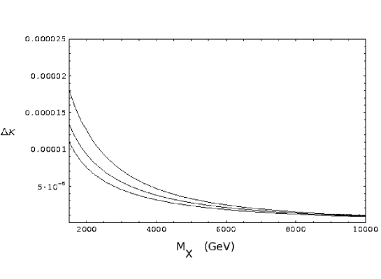
Figure 3: CMDM as a function of the bilepton gauge boson mass for three values of the $J_{3}$: 1, 2, 3 TeV.

	$A$	$B$	$A^{{}^{\prime}}$	$B^{{}^{\prime}}$
$tJ_{3}G_{Y}$	$-i\frac{gm_{J}}{\sqrt{2}M_{X}}$	0	0	$-i\frac{gm_{J}}{\sqrt{2}M_{X}}$
$tJ_{3}Y_{\mu}$	$-i\frac{g}{\sqrt{2}}$	0	$-i\frac{g}{\sqrt{2}}$	0
$ttZ^{\prime}_{\mu}$	$-i\frac{g(1+t_{W}^{2})}{2\sqrt{3}\sqrt{1-3t_{W}^{2}}}$	$-i\frac{2g}{\sqrt{3}\sqrt{1-3t_{W}^{2}}}$	$-i\frac{g(1+t_{W}^{2})}{2\sqrt{3}\sqrt{1-3t_{W}^{2}}}$	$-i\frac{2g}{\sqrt{3}\sqrt{1-3t_{W}^{2}}}$
$tJ_{3}X$	$i\frac{g}{\sqrt{2}}$	0	$i\frac{g}{\sqrt{2}}$	0

Table 3: Feynman rules for the 331 model contributions to the CMDM

II.4 Topcolor Assisted Technicolor

Light particles of the SM can be regarded as spectators of the electroweak symmetry breaking and the massive top quark suggests that it is playing an important role in the dynamics. This implies the possibility of a new interaction which drives the EWSB and the big top mass in order to distinguish the top quark from the other fermions. This interaction can generate desviations of the top quark properties from the SM predictions.

In the topcolor scenario diecisiete ; dieciocho ; diecinueve ; veinte , the EWSB mechanism arises from a new, strongly coupled gauge interaction at TeV energy scales. In the TC2 model diecisiete , the topcolor interaction generates the top quark condensation that gives rise to the main part of the top-quark mass $(1-\varepsilon)m_{t}$, with the model dependent parameter $\varepsilon$ fixed in the range $0.03<\varepsilon<0.1$ diecinueve . This model predicts three heavy top-pions $(\pi^{0}_{t},\pi^{\pm}_{t})$ and one top-Higgs boson $h^{0}_{t}$ with large Yukawa couplings to the third generation of fermions. The respective Yukawa couplings are obtained from the Lagrangian

$${\cal L}=\mid D_{\mu}\Phi\mid^{2}-Y_{t}\frac{\sqrt{v_{w}^{2}-F_{t}^{2}}}{v_{w}}\overline{\Psi}_{L}\Phi t_{R}-Y_{t}\frac{\sqrt{v_{w}^{2}-F_{t}^{2}}}{v_{w}}\overline{t}_{R}\Phi\Psi_{L}-m_{t}\overline{t}t,$$ (28)

with $Y_{t}=(1-\varepsilon)m_{t}/F_{t}$, $\nu_{\omega}=\nu/\sqrt{2}\approx 174GeV$, and the scalar field $\Phi$ is given by

$$\Phi=\left(\begin{array}[]{c}\frac{1}{\sqrt{2}}(h^{0}_{t}+i\pi_{t}^{0})\\ \pi_{t}^{+}\end{array}\right).$$ (29)

For the purpose of the present paper, we will take the following values for the topcolor parameters: $\varepsilon=0.1$, $\nu_{\omega}=174$ GeV and $F_{t}=50$ GeV. The Feynman rules for this model are depicted in Table IV.

	$A$	$B$	$A^{{}^{\prime}}$	$B^{{}^{\prime}}$
$tth_{t}^{0}$	$-i\frac{(1-\epsilon)m_{t}}{\sqrt{2}v_{w}}F$	$-i\frac{(1-\epsilon)m_{t}}{\sqrt{2}v_{w}}F$	$-i\frac{(1-\epsilon)m_{t}}{\sqrt{2}v_{w}}F$	$-i\frac{(1-\epsilon)m_{t}}{\sqrt{2}v_{w}}F$
$tt\pi_{t}^{0}$	$-\frac{(1-\epsilon)m_{t}}{\sqrt{2}v_{w}}F$	$\frac{(1-\epsilon)m_{t}}{\sqrt{2}v_{w}}F$	$-\frac{(1-\epsilon)m_{t}}{\sqrt{2}v_{w}}F$	$\frac{(1-\epsilon)m_{t}}{\sqrt{2}v_{w}}F$
$tb\pi_{t}^{+}$	$0$	$-i\frac{(1-\epsilon)m_{t}}{v_{w}}F$	$-i\frac{(1-\epsilon)m_{t}}{v_{w}}F$	0

Table 4: Feynman rules for the TC2 model contributions to the CMDM, with $F=\sqrt{\frac{v_{w}^{2}}{F_{t}^{2}}-1}$

The masses of the top-Higgs scalars $\pi^{0}_{t}$ and $\pi^{+}_{t}$ are almost degenerate since they differ only by small electroweak corrections veinte . We will take for the top-Higgs mass a value bigger than twice the value of the mass of the top-quark veinte .

In Figure 4 we present the evolution of each one of the topcolor scalars $h^{0}_{t},\pi^{\pm}_{t},\pi^{0}_{t}$ contributions to the CMDM as function of their masses. In Figure 5 we compare the topcolor and the SM contributions to the top-quark CMDM.

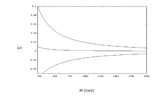
Figure 4: CMDM as function of the topcolor particle masses: the curve at the top corresponds to $h^{0}_{t}$, the one at the middle to $\pi^{+}_{t}$ and the bellow to $\pi_{t}^{0}$

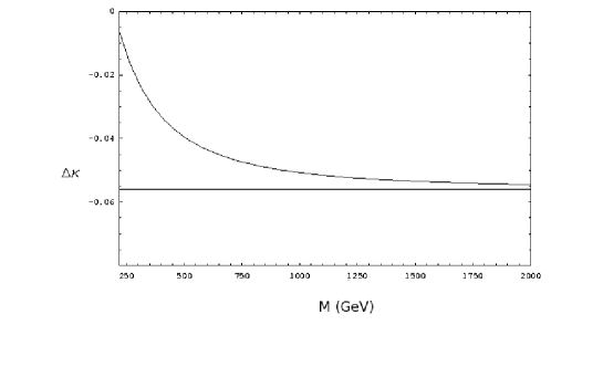
Figure 5: CMDM as function of the topcolor particle mass: the horizontal line corresponds to the SM prediction and the line at the top gives the total topcolor TC2 predictions.

For $m_{h^{0}_{t}}\approx m_{\pi_{t}}\approx m_{\pi_{0}}\approx 250$ GeV and summing the respective value for the SM, we find

$$\Delta\kappa^{TC2}_{(s)}=-0.01,$$ (30)

which is of the order of the sensibility of the LHC.

There is a previous estimate of the contribution to the CMDM induced by a techniscalar in TC2 models tres . However, this estimate did not consider the actual suppression factors $(4\pi)^{-2}$ involved in one-loop calculations and it was obtained a rather large value for this contribution, of order 0.1, even for a relatively massive techniscalar (0.5 TeV) tres .

II.5 Universal Extra Dimensions

We consider a generalization of the SM where all the particles propagate in five dimensions: $x=0,1,2,3$ correspond to the usual coordinates and $x^{5}=y$ is the fifth one. This extra dimension will be compactified in a circle of ratio $R$ with the points $y$ and $-y$ identified in a $S^{1}/Z_{2}$ orbifold veintiuno ; veintidos . The terms that will contribute at the one-loop order to the CMDM are given by

$$L=\int d^{4}xdy({\cal L}_{F}+{\cal L}_{Y})$$ (31)

with

$${\cal L}_{F} = \left[\overline{Q}i\Gamma^{M}D_{M}Q+\overline{U}i\Gamma^{M}D_{M}U+\overline{D}i\Gamma^{M}D_{M}D\right],$$

$${\cal L}_{Y} = -\overline{Q}\lambda_{u}\widetilde{\Phi}U-\,\overline{Q}\lambda_{d}\Phi D+h.c.$$ (32)

The numbers $M,N=0,1,2,3,5$ denote the five dimensional Lorentz indexes. The covariant derivative is defined as $D_{M}\equiv\partial_{M}+i\widehat{g}W^{a}_{M}T^{a}+i\widehat{g}\,^{\prime}B_{M}Y$. The five dimensional gamma matrices $\Gamma_{M}$ are $\Gamma_{\mu}=\gamma_{\mu}$ and $\Gamma_{4}=i\gamma_{5}$ with the metric tensor given by $g_{MN}=(+,-,-,-,-)$.

The Fourier expansions of the fields are given by:

$$B_{\mu}(x,y) = \frac{1}{\sqrt{\pi R}}B_{\mu}^{(0)}(x)+\frac{\sqrt{2}}{\sqrt{\pi R}}\sum_{n=1}^{\infty}B_{\mu}^{(n)}(x)\cos\left(\frac{n\pi y}{R}\right),$$

$$B_{5}(x,y) = \frac{\sqrt{2}}{\sqrt{\pi R}}\sum_{n=1}^{\infty}B_{5}^{(n)}(x)\sin\left(\frac{n\pi y}{R}\right),$$ (33)

$$Q(x,y) = \frac{1}{\sqrt{\pi R}}Q_{L}^{(0)}(x)+\frac{\sqrt{2}}{\sqrt{\pi R}}\sum_{n=1}^{\infty}\left[Q_{L}^{(n)}(x)\cos\left(\frac{n\pi y}{R}\right)+Q_{R}^{(n)}\sin\left(\frac{n\pi y}{R}\right)\right],$$

$$U(x,y) = \frac{1}{\sqrt{\pi R}}U_{R}^{(0)}(x)+\frac{\sqrt{2}}{\sqrt{\pi R}}\sum_{n=1}^{\infty}\left[U_{t\;R}^{(n)}(x)\cos\ \left(\frac{n\pi y}{R}\right)+U_{t\;L}^{(n)}\sin\left(\frac{n\pi y}{R}\right)\right]$$

The expansions for $B_{\mu}$ and $B_{5}$ are similar to the expansions for all the gauge fields and the Higgs doublet (but this last one without the $\mu$ or $5$ Lorentz index). It is by integrating the fifth $y$ component that we obtain the usual interaction terms and the KK spectrum for ED models, $Q^{(n)}=\left(Q^{(n)}_{t}\;\;\;Q^{(n)}_{b}\right)^{T}$.

	$A$	$B$	$A^{{}^{\prime}}$	$B^{{}^{\prime}}$
$t^{(0)}A^{(n)}_{\mu}Q_{t}^{(n)}$	$i\frac{2}{3}e$	0	$i\frac{2}{3}e$	0
$t^{(0)}Z^{(n)}_{\mu}Q_{t}^{(n)}$	$i\frac{g}{c_{W}}(\frac{1}{2}-\frac{2}{3}s_{W}^{2})$	0	$i\frac{g}{c_{W}}(\frac{1}{2}-\frac{2}{3}s_{W}^{2})$	0
$t^{(0)}W^{(n)}_{\mu}Q_{b}^{(n)}$	$i\frac{g}{\sqrt{2}}$	0	$i\frac{g}{\sqrt{2}}$	0
$t^{(0)}A^{(n)}_{\mu}U_{t}^{(n)}$	0	$i\frac{2}{3}e$	0	$i\frac{2}{3}e$
$t^{(0)}Z^{(n)}_{\mu}U_{t}^{(n)}$	0	$i\frac{2}{3}g\frac{s_{W}^{2}}{c_{W}}$	0	$i\frac{2}{3}g\frac{s_{W}^{2}}{c_{W}}$

Table 5: Feynman rules for gauge KK of the UED contributions to the CMDM of top quark

We will be interested in the third family of quarks and $Q_{t}^{(n)}$ and $Q_{b}^{(n)}$ will refer to the upper and lower parts of the doublet $Q$. Similarly, the $U_{t}^{(n)}$ and $D_{t}^{(n)}$ will be the KK modes of the usual right-handed singlet top quarks. There is a mixing between the masses of the gauge eigenstates of the KK top quarks ($Q_{t}^{(n)}$ and $U_{t}^{(n)}$), where the mixing angle is given by $\tan(2\alpha_{t}^{n})=m_{t}/m_{n}$ with $m_{n}\approx n/R$. However, we will neglect this mixing angle $(\sin\alpha_{t}=0)$ for the purpose of the present calculation.

	$A$	$B$	$A^{{}^{\prime}}$	$B^{{}^{\prime}}$
$t^{(0)}A^{(n)}_{5}Q_{t}^{(n)}$	$-\frac{2}{3}e$	0	0	$\frac{2}{3}e$
$t^{(0)}Z^{(n)}_{5}Q_{t}^{(n)}$	$-\frac{g}{c_{W}}(\frac{1}{2}-\frac{2}{3}s_{W}^{2})$	0	0	$\frac{g}{c_{W}}(\frac{1}{2}-\frac{2}{3}s_{W}^{2})$
$t^{(0)}W^{(n)}_{5}Q_{b}^{(n)}$	$-\frac{g}{\sqrt{2}}$	0	0	$\frac{g}{\sqrt{2}}$
$t^{(0)}A^{(n)}_{5}U_{t}^{(n)}$	0	$\frac{2}{3}e$	$-\frac{2}{3}e$	0
$t^{(0)}Z^{(n)}_{5}U_{t}^{(n)}$	$-\frac{2}{3}g\frac{s_{W}^{2}}{c_{W}}$	0	0	$\frac{2}{3}g\frac{s_{W}^{2}}{c_{W}}$

Table 6: Feynman rules for KK scalar of the UED contributions to the CMDM of top quark

	$A$	$B$	$A^{{}^{\prime}}$	$B^{{}^{\prime}}$
$t^{(0)}A^{a,(n)}_{\mu}Q_{t}^{(n)}$	$ig_{s}$	0	$ig_{s}$	0
$t^{(0)}A^{a,(n)}_{\mu}U_{t}^{(n)}$	0	$ig_{s}$	0	$ig_{s}$
$t^{(0)}A^{a,(n)}_{5}Q_{t}^{(n)}$	$g_{s}$	0	0	$-g_{s}$
$t^{(0)}A^{a,(n)}_{5}U_{t}^{(n)}$	0	$-g_{s}$	$g_{s}$	0

Table 7: Feynman rules for the KK states for the QCD contributions to the CMDMT

In table V we include the Feynman rules for the fifth component of a gauge field, the KK scalar which will induce the UED contribution to the CMDM of the top quark (Figure 1a). Table VI contains the respective Feynman rules for the couplings of the external quark $t$ which corresponds to the $t^{(0)}$ component with a gauge and quark excitations (Fig. 1a). Table VII includes the respective Yukawa couplings for an external quark $t^{(0)}$ with the scalar $KK$ states (Fig. 1a). Finally, the couplings presented in Table 8 will be used to compute the QCD contribution to the CMDM induced by the $KK$ excitations associated to the fifth component of the gluon field $A^{Q,(n)}_{5}$ (Figs. 1a and 2a).

Here we will take $1/R\approx 1$ TeV. The $KK$ modes corresponding to the EW sector for the gauge (Table (5)) and scalar (Table (6)) in the loop, respectively, then give the following contribution to the CMDM

$$\Delta\kappa_{(\mu)}^{EW,5D} = -1.3\times 10^{-4}$$

$$\Delta\kappa_{(s)}^{EW,5D} = -4.1\times 10^{-4}$$ (34)

with a total value for the electroweak contribution given by

$$\Delta\kappa^{EW,5D}=-5.4\times 10^{-4}$$ (35)

The KK modes of the QCD sector induces the following contributions

$$\Delta\kappa_{(\mu)}^{QCD,5D} = -9.4\times 10^{-4}$$

$$\Delta\kappa_{(s)}^{QCD,5D} = -8.2\times 10^{-4}$$ (36)

corresponding to the gauge and scalar excitations contribution, respectively, which add to the following value

$$\Delta\kappa^{QCD,5D}=-1.8\times 10^{-3}$$ (37)

Adding the EW eq. (35) and QCD eq. (37) contributions we get finally

$$\Delta\kappa^{5D}=-2.3\times 10^{-3}.$$ (38)

III CONCLUDING REMARKS

In conclusion, we have made a critical analysis of the one loop calculations for the CMDM of the top quark model. Our new results differ slighty from those already published for the SM and the THDM nueve . In the TC2 model, our one-loop computation shows a smaller value for the CMDM then the one previously obtained tres , which in turn is also in agreement with the constraints obtained from low-energy precision experiments nueve . As far as we know, the one-loop calculations for the 331 and universal extra-dimensions models have not been performed previously. In particular, the 331 result is suppressed by two orders of magnitud with respect to the SM result and the extra-dimensions result is also in agreement with the low-energy precision contraints. In this respect, a precise measurement of the top-quark CMDM may be used to distinguish between competing extensions of the SM. If we sum to the SM CMDM the additional contributions given for the different models considered in the present paper, we get the following results

$$\Delta\kappa^{SM} = -5.6\times 10^{-2}\;\;,\;\;\Delta\kappa^{THDM}=-5.1\times 10^{-2}$$

$$\Delta\kappa^{TC2} = -1.0\times 10^{-2}\;\;,\;\;\Delta\kappa^{5D}=-5.8\times 10^{-2}.$$ (39)

Finally, eventhough the effects induced at NLO QCD corrections on top quark production and decays have already been studied veintitres , as far as we know the complete NLO QCD corrections to the CMDM $\Delta\kappa$ of the top quark have not been calculated in any of these models. It is important also to point out that the angular distributions of leptons or jets due to $t\bar{t}$ spin correlations allow a determination of the CMDM of the top quark with an accuracy of order 0.1 veintecinco . This method provides a competitive way to observe new physics contributions to the CMDM, which is stable against experimental uncertainties veintecinco .

Appendix A CMDM ANAYLTICAL EXPRESSIONS

In this appendix we present the analytical expressions obtained for each one-loop Feynman diagram involved in the calculation of the top-quark CMDM. We have used these expressions in order to perform the respective numerical calculations that lead to the CMDM results presented in this paper. This method has already been used to compute higher order corrections to fermion vertices or flavor-changing neutral vertices involving leptons or the top quark Deshapande .

The Feynman diagram shown on Fig. 1a corresponds to the scalar contribution to the top-quark CMDM. In the SM, the scalars circulating in the loop can be $h^{0}$, $G_{Z}$, and $G_{W}$, while in the 331 models it is $G_{X}$. In the UED models, this contribution arises from the scalar $KK$ excitations $h^{0,(n)},G^{(n)}_{Z},....$, and fifth component of the gauge fields $A^{(n)}_{5},Z^{(n)}_{5},W^{(n)}_{5}$. The respective QCD excitations for the $KK$ sector correspond to $A^{a,(n)}_{5}$. We will use the following notation for the incoming and the outcoming scalar couplings involved in Fig. 1a, respectively

$$(AP_{L}+BP_{R})T^{a}\;\;\;,\;\;\;(A^{\prime}P_{L}+B^{\prime}P_{R})T^{a}$$ (40)

where $T^{a}$ corresponds to the $SU(3)_{C}$ generators in the case of QCD scalar loop and it is just the unit matrix otherwise.

The contribution to the CMDM arising from the diagram given in Fig. 1a is thus given by the expression,

$$\Delta\kappa^{QCD}_{(s)} = -\frac{1}{6\times 8\pi^{2}}\int_{0}^{1}dx\int_{0}^{1-x}dy\frac{1}{(x+y)^{2}+(x+y)(\widehat{M}^{2}-\widehat{m}^{2}-1)+\widehat{m}^{2}}$$ (41)

$$\times \{(x+y)(x+y-1)(B^{\prime}A+A^{\prime}B)-\widehat{M}(x+y)(A^{\prime}A+B^{\prime}B)\}$$

where $m(M)$ correspond to the scalar (fermion) mass in the loop and the factor (-1/6) comes from the $SU(3)_{C}$ generator algebra, and $\widehat{m}=m/m_{t}$ is the normalized top-quark mass. In order to get the respective EW scalar contribution for Fig. 1a, we have to replace the factor (-1/6) by the unit and take the appropriated scalar couplings.

In particular, if we set $A=B=A^{{}^{\prime}}=B^{{}^{\prime}}=1$ and $\widehat{M}=1$ in Eq. (A.2), we get directly the $h^{0}$ contribution to $\Delta\kappa_{(5)}$ which agrees with the result given in Eq. (A.10) of Fujikawa et al. Fujikawa . On the other hand, if we set $A=A^{{}^{\prime}}=-B=-B^{{}^{\prime}}=1$ and $\widehat{M}=1$ in our Eq. (A.2), we get the respective pseudoscalar $G_{Z}$ contribution which also agrees with Eq. (3.5) of Ref. Fujikawa .

If we have two $KK$ excitations running in the loop of Fig. 1a, the respective analytical expression is given by

$$\Delta\kappa_{(s)} \approx -\sum_{n=1}^{\infty}\frac{1}{12\times 48\pi^{2}}\frac{1}{\widehat{(n/R)}^{2}}\{3(B^{\prime}A+A^{\prime}B)-2\widehat{M}(A^{\prime}A+B^{\prime}B)\}$$ (42)

$$\approx -\frac{\widehat{R}^{2}}{72\times 48}\{3(B^{\prime}A+A^{\prime}B)-2\widehat{M}(A^{\prime}A+B^{\prime}B)\},$$

where we have used the approximation that the masses of both excitations are of the same order of magnitude $m_{n}\sim n/R$ and we have neglected any other mass circulating in the loop.

The diagram shown in Fig. 1b receives contributions from the SM gauge bosons W, Z, g, the 331 gauge boson X, and for the UED model it can be the respective EW or QCD gauge bosons $A^{(n)}_{\mu},Z^{(n)}_{\mu},W^{(n)}_{\mu}$ and $A^{a,(n)}_{\mu}$. In this case, we use the following notation for the gauge and fermionic couplings involved in this diagram,

$$\gamma_{\alpha}(AP_{L}+BP_{R})T^{a}\;\;\;\;\;\;\gamma_{\alpha}(A^{\prime}P_{L}+B^{\prime}P_{R})T^{a},$$ (43)

where the $T^{a}$ correspond again to the $SU(3)_{C}$ generators. The respective analytical expression for this contribution is given by,

$$\Delta\kappa_{(\mu)} = -\frac{1}{6\times 4\pi^{2}}\int_{0}^{1}dx\int_{0}^{1-x}dy\frac{1}{(x+y)^{2}+(x+y)(\widehat{M}^{2}-\widehat{m}^{2}-1)+\widehat{m}^{2}}$$ (44)

$$\times \{(x+y-2)(x+y-1)(A^{\prime}A+B^{\prime}B)$$

$$- \widehat{M}(x+y-1)(A^{\prime}B+B^{\prime}A)\}.$$

$$\Delta\kappa_{(\mu)} \approx -\sum_{n=1}^{\infty}\frac{1}{12\times 24\pi^{2}}\frac{1}{(\widehat{n/R})^{2}}\{3(A^{\prime}A+B^{\prime}B)-2\widehat{M}(A^{\prime}B+B^{\prime}A)\}$$ (45)

$$\approx -\frac{\widehat{R}^{2}}{72\times 24}\{3(A^{\prime}A+B^{\prime}B)-2\widehat{M}(A^{\prime}B+B^{\prime}A)\},$$

In order to get the EW contribution for the diagram 1b, we have to make the same sustitutions indicated for the expression (A.2).

For example, if we apply Eq. (A.5) to the loop induced by the exchange of a $Z$ gauge boson and set $\widehat{M}=1$, we get direclty Eq. (A.4) of Fujikawa et al. Fujikawa with $\eta=1$. For the loop induced by the exchange of a gluon, if we set $\widehat{M}=1$ $\widehat{m}=0$, and $A=B=A^{{}^{\prime}}=B^{{}^{\prime}}=-ig_{s}$, we obtain

$$\Delta\kappa^{QCD}_{(\mu)}=-\frac{1}{6}\frac{\alpha_{s}}{\pi}.$$ (46)

The above result reduces to the well known QED result $\Delta\kappa=\alpha/(2\pi)$ if we supress the factor $-1/6$ coming from $SU(3)_{C}$ algebra and an additional $1/2$ factor which was introduced in the definition of $\Delta\kappa$ given in Eq. (1).

In the UED models, the diagram shown in Fig. 2a receives contributions from a colored scalar particle which corresponds to the dimension 5 component of the gluons, $A^{a,(n)}_{5}$. In this case we use the following notation for the respective couplings,

$$(AP_{L}+BP_{R})T^{c}\;\;\;,\;\;\;(A^{\prime}P_{L}+B^{\prime}P_{R})T^{d}.$$ (47)

where the couplings for the excitated colored scalar with the external gluon may be taken from Ref.diecinueve . The corresponding contribution has the analytical expression,

$$\Delta\kappa_{(s)} = \frac{3}{16\pi^{2}}\int_{0}^{1}dx\int_{0}^{1-x}dy\frac{1}{(x+y)^{2}+(x+y)(\widehat{M}^{2}-\widehat{m}^{2}-1)+\widehat{m}^{2}}$$ (48)

$$\times \{(x+y)(x+y-1)(A^{\prime}B+B^{\prime}A)$$

$$- \widehat{m}(x+y-1)(A^{\prime}A+B^{\prime}B)\}$$

and in this case the factor 3/2 comes from the Lie algebra of the generators $f^{abc}T^{b}T^{c}$. The expression for the $KK$ contributions in this case reduces to

$$\Delta\kappa_{(s)} \approx -\sum_{n=1}^{\infty}\frac{3}{12\times 16\pi^{2}}\frac{1}{(\widehat{n/R})^{2}}\{3(A^{\prime}B+B^{\prime}A)+2\widehat{M}(A^{\prime}A+A^{\prime}A)\}$$ (49)

$$\approx \frac{\widehat{R}^{2}}{24\times 16}\{3(A^{\prime}B+B^{\prime}A)+2\widehat{M}(A^{\prime}A+B^{\prime}B)\},$$

where we have assumed again that the the excitation masses running in the loop are of the same order of magnitude.

The diagram given in Fig. 2b receives contributions from the gluons $A^{a}_{\mu}$ or the respective $KK$ excitations $A^{a,(n)}_{\mu}$, the notation for the respective couplings is given by

$$\gamma_{\alpha}(AP_{L}+BP_{R})T^{a}\;\;\;\;\;\;\gamma_{\beta}(A^{\prime}P_{L}+B^{\prime}P_{R})T^{b}$$ (50)

and thus the corresponding QCD contribution to the CMDM may be expressed as

$$\Delta\kappa_{(\mu)} = \frac{3}{8\pi^{2}}\int_{0}^{1}dx\int_{0}^{1-x}dy\frac{1}{(x+y)^{2}+(x+y)(\widehat{M}^{2}-\widehat{m}^{2}-1)+\widehat{m}^{2}}$$ (51)

$$\times \{(x+y)(x+y-1)(A^{\prime}A+B^{\prime}B)$$

$$- \widehat{M}(x+y-1)(A^{\prime}B+B^{\prime}A)\}$$

Finally, if we have two $KK$ excitations running in this loop, we get the following expression for this contribution

$$\Delta\kappa_{(\mu)} = \frac{3}{8\pi^{2}}\int_{0}^{1}dx\int_{0}^{1-x}dy\frac{1}{(x+y)^{2}+(x+y)(\widehat{M}^{2}-\widehat{m}^{2}-1)+\widehat{m}^{2}}$$ (52)

$$\times \{(x+y)(x+y-1)(A^{\prime}A+B^{\prime}B)$$

$$- \widehat{M}(x+y-1)(A^{\prime}B+B^{\prime}A)\}.$$

Acknowledgments

This work was supported by Fundación Banco de la República (Colombia), CONACyT (México) and the HELEN proyect.

References

• (1) CDF/DO Collab., http://www-cdf.fnal.gov/physics/new/top/top.html
• (2) J.A. Aguilar-Saavedra, Acta Phys. Pol. B35 2695 (2004).
• (3) D. Atwood, A. Kagan and T.G. Rizzo, Phys. Rev. D52, 6264 (1995); T.G. Rizzo, Phys. Rev. D50, 4478 (1994); J.L. Hewett and T.G. Rizzo, Phys. Rev. D49, 319 (1994); J.L. Hewett, Int. J. Mod. Phys. A13, 2389 (1989).
• (4) K. Whisnant et al., Phys. Rev.D56, 467 (1997); J.M. Yang and B.-L. Young, Phys. Rev.D56, 5907 (1997); K. Hikasa et al., Phys. Rev.D58, 114003 (1998).
• (5) K. Cheung, Phys. Rev. D53, 3604 (1996); P. Haberl et al., Phys. Rev.D53 4875 (1996); T. Rizzo, ibid. 6218 (1996).
• (6) D. Silverman and G. Shaw, Phys. Rev. D27, 1196 (1983); J.M. Yang and C.S. Li, Phys.D52, 1541 (1991); ibid 54, 4380 (1996); C.S. Li, O. Oakes and J.M. Yang, ibid 55, 1672 (1997) .
• (7) F. Abe et al., CDF Coll., Phys. Rev. Lett. 80, 2525 (1998); T. Han et al., Phys. Lett.B385, 311 (1996).
• (8) F. del Aguila, Acta Phys. Pol.B30, 3303 (1999); J.A. Aguilar-Saavedra, Acta Phys. Pol.B35, 2695 (2004).
• (9) R. Martinez and J.A. Rodriguez, Phys. Rev.D65, 057301 (2002); Phys. Rev.D55, 3212 (1997); R. Martinez, J.A. Rodriguez and M. Vargas, D60, 077504-1 (1999).
• (10) F. Larios, M.A. Pérez and C.P. Yuan, Phys Lett. B457, 334 (1999).
• (11) R. Martinez, M.A. Pérez and J.J. Toscano, Phys. Lett. B340, 91 (1994); T. Han et al., Phys. Rev.D55, 7241 (1997); F. Larios, R. Martinez and M.A. Pérez, Phys. Rev. D72, 057504 (2005); Int. J. Mod. Phys. A21, 3473 (2006).
• (12) A. Brandenburg and J.P. Ma, Phys. Lett. B298, 211 (1993). E.O. Iltan, Phys. Rev. D65, 073013 (2002); P. Haberl, O. Nachtmann and A. Wilch, Phys. Rev. D53, 4875 (1996).
• (13) S.L.Glashow, Nucl. Phys. 22, 579 (1961); S. Weinberg, Phys. Rev. Lett. 19, 1264 (1964); A. Salam, in Elementary Particle Theory (Nobel Symposium Nr. 8), edited by N. Svartholm, Almqvist and Wiksell, Stckholm, Sweden (1968).
• (14) J. Gunion, H. Haber, G. Kane and S. Dawson, The Higgs Hunter’s Guide, (Addison-Wesley, New York, 1990); R. A. Díaz, R. Martínez and J.-Alexis Rodríguez, Phys. Rev. D64, 033004 (2001); Phys. Rev. D63, 095500 (2001).
• (15) R.A. Diaz, R. Martinez and F. Ochoa, Phys. Rev. D69, 095009 (2004).
• (16) R. Foot, F. Hernández, F. Pisano and V. Pleitez, Phys. Rev. D47, 4158 (1993); V. Pleitez and M.D. Tonasse, Phys. Rev. D48, 2353 (1993); T.V. Duong and E. Ma, Phys. Lett. B316, 307 (1993); G.A. Gonzalez-Sprinberg, R. Martinez and O. Sampayo, Phys. Rev. D71 11503 (2005).
• (17) H. N. Long, P. B. Pal, Mod. Phys. Lett.A13, 2355 (1998); N. T. Anh, N. A. Ky, H. N. Long, Int. J. Mod. Phys. A16, 541 (2001).
• (18) T.C. Hill, Phys. Lett. B345, 483 (1995); K. Lane and E. Eichten, Phys. Lett. B352, 382 (1995); K. Lane, Phys. Lett. B433, 96 (1998); G. Cvetic, Rev. Mod. Phys. 71 513 (1999).
• (19) C.T. Hill, Phys. Lett.B266, 419 (1991).
• (20) G. Burdman, Phys. Rev. Lett. 83, 2888 (1999); W.A. Bardeen, C.T. Hill and M. Linder, Phys. Rev. D41, 1647 (1990).
• (21) B. Balaji, Phys. Lett. B393, 89 (1997); G. Burdman and D. Kominis, Phys. Lett. B403, 101 (1997); C. Yue, Y.P. Kuang, X. Wang and W. Li, Phys. Rev. D62, 055005 (2000); A.K. Leibovich and Rainwater, Phys. Rev. D65, 055012 (2002).
• (22) A. Muck, A. Pilaftsis and R. Ruckl, hep-ph/0209371.
• (23) W. Bernreuther et, al., Int. J. Mod. Phys. A18, 1357 (2003); hep-ph/0209202.
• (24) B. Holdom and T. Torma, Phys. Rev. D60, 114010 (1999).
• (25) N.G. Deshapande, M. Nazerimonfared, Nucl. Phys. B213, 390 (1983); J.L. Diaz-Cruz et al., Phys. Rev. D41, 891, 1990); R. Martinez, M.A. Perez, Phys. Lett. B340, 91 (1994); F. Larios, R. Martinez, M.A. Perez, Phys. Lett. B345, 259 (1995); R. Martinez, J.A. Rodriguez, Phys. Rev. D55, 3212 (1997); R.A. Diaz, R. Martinez, J.A. Rodriguez, Phys. Rev. D64, 033004 (2001); M.A. Perez, G. Tavares-Velasco, J.J. Toscano, Int. J. Mod. Phys. A19, 159 (2004); F. Larios, R. Martinez, M.A. Perez, Int. J. Mod. Phys. A21, 3473 (2006).
• (26) K. Fujikawa, B.W. Lee and A.I. Sanda, Phys. Rev. D6 2923 (1972).