The production of the new gauge boson $B_{H}$ via $e^{-}\gamma$ collision in the littlest Higgs model

Abstract

The new lightest gauge boson $B_{H}$ with mass of a few hundred GeV is predicted in the littlest Higgs model. $B_{H}$ should be accessible in the planed ILC and the observation of such particle can strongly support the littlest Higgs model. The realization of $\gamma\gamma$ and $e\gamma$ collision will open a wider window to probe $B_{H}$. In this paper, we study the new gauge boson $B_{H}$ production processes $e^{-}\gamma\rightarrow e^{-}\gamma B_{H}$ and $e^{-}\gamma\rightarrow e^{-}ZB_{H}$ at the ILC. Our results show that the production cross section of the process $e^{-}\gamma\rightarrow e^{-}ZB_{H}$ is less than one fb in the most parameter spaces while the production cross section of the process $e^{-}\gamma\rightarrow e^{-}\gamma B_{H}$ can reach the level of tens fb and even hundreds of fb in the sizable parameter spaces allowed by the electroweak precision data. With the high luminosity, the sufficient typical signals could be produced, specially via $e^{-}\gamma\rightarrow e^{-}\gamma B_{H}$. Because the final electron and photon beams can be easily identified and the signal can be easily distinguished from the background produced by $Z$ and $H$ decaying, $B_{H}$ should be detectable via $e\gamma$ collision at the ILC. Therefore, the processes $e^{-}\gamma\rightarrow e^{-}\gamma B_{H}$ and $e^{-}\gamma\rightarrow e^{-}ZB_{H}$ provide a useful way to detect $B_{H}$ and test the littlest Higgs model.

PACS number(s): 12.60.Cn, 14.80.Cp,13.66.Hk,11.30.Na

I. Introduction  

The Standard Model (SM) of particle physics is a remarkably successful theory. It provides a complete description of physics at currently accessible energy, and its predictions have been confirmed to high accuracy by the high energy experiments. However, the mechanism of electroweak symmetry breaking(EWSB) remains unknown. Furthermore, in the SM, the Higgs mass receives quadratically divergent quantum corrections which have to be cancelled by some new physics(NP) to avoid fine-tuning. The SM Higgs sector is therefore an effective theory below some cut-off scale $\Lambda$. To avoid fine-tuning of Higgs mass, one would require the NP scale $\Lambda$ to be $\sim$ TeV. Various NP models were proposed at the TeV scale, which can cancel the quadratic divergences of the SM Higgs. Recently, a new theory, dubbed the little Higgs theory[1], has drawn a lot of interests as a new candidate for solution of the problems mentioned above.

So far, a number of specific little Higgs models [2, 3, 4, 5] have been proposed. The generic structure of these models is that a global symmetry is broken at the scale f which is around a TeV. At the scale f there are new gauge bosons, scalars, fermions responsible for canceling the one loop quadratic divergences to the Higgs mass from the SM particles. The new particles predicted by the little Higgs models will emerge characteristic signatures at the present or future high energy collider experiments[6]. Furthermore, among the various little Higgs models, the most economical and phenomenologically viable model is the littlest Higgs model[5] which realizes the little Higgs idea and has all essential features of the little Higgs models. Such model consists of a nonlinear $\sigma$ model with a global SU(5) symmetry which is broken down to SO(5) by a vacuum expectation value (vev) of order f $\sim\Lambda_{s}/4\pi\sim$ TeV. At the same time, the gauge subgroup $[SU(2)\times U(1)]^{2}$ is broken to its diagonal subgroup $SU(2)\times U(1)$, identified as the SM electroweak gauge group. This breaking scenario gives rise to four massive gauge bosons $(B_{H},Z_{H},W^{\pm}_{H})$. Thus, studying the possible signatures of the new gauge bosons and their contribution to some processes at high-energy colliders is a good method to test the littlest Higgs model and furthermore to probe the EWSB mechanism. However, in the littlest Higgs model, the masses of these new heavy gauge bosons are in the range of a few TeV, except for the mass of $B_{H}$ in the range of hundreds GeV. In fact, the gauge boson $B_{H}$ is the lightest new particle in the littlest Higgs model so that it should be the first signal at future experiments and would play the most important role in probing the littlest Higgs model.

It is well known that the LHC can directly probe the possible NP beyond the SM up to a few TeV. If the new particles or interactions will be directly discovered at the future hadron collider experiments, the linear $e^{+}e^{-}$ collider(LC) will then play a crucial role in the detailed and thorough study of these new phenomena and in the reconstruction of the underlying fundamental theories. In addition $e^{+}e^{-}$ physics, the future LC provides a unique opportunity to study $\gamma\gamma$ and $e\gamma$ interactions at high energy and luminosity comparable to those in $e^{+}e^{-}$ collisions[7]. High energy photons for $\gamma\gamma$, $e\gamma$ collisions(Photon Collider) can be obtained using Compton backscattering of laster light off the high energy electrons. Such possibilities will be realized at the International Linear Collider(ILC), with the center of mass(c.m.) energy $\sqrt{s}$=300 GeV-1.5 TeV and the yearly luminosity 500 $fb^{-1}$[8]. The physics potential of the Photon Collider is very rich and complements the physics program of the $e^{+}e^{-}$ mode. The Photon Collider will considerably contribute to the detailed understanding of new phenomena, and in some scenarios it is the best instrument for the discovery of elements of NP. In particular, the $e^{-}\gamma$ collision can produce particles which are kinematically not accessible at $e^{+}e^{-}$ collisions at the same collider[7, 9]. Moreover, the high energy photon polarization can vary relatively easily, which is advantageous for experiments. All the virtues of the Photon Collider will provide us with a good chance to pursue NP particles, specially the lightest new gauge boson $B_{H}$ which should be kinematically accessible at the planned ILC. Some $B_{H}$ production processes have been studied at the Photon Collider[10, 11]. In the reference[10], we have studied a process of the $B_{H}$ production associated with W boson pair via photon-photon collision, i.e., $\gamma\gamma\rightarrow W^{+}W^{-}B_{H}$. Such process would offer a good chance to probe the $B_{H}$ signal and to study the triple and quartic gauge couplings involving $B_{H}$ and the SM gauge bosons which shed important light on the symmetry breaking features of the littlest Higgs model. Via $e\gamma$ collision, a single heavy new gauge boson in the littlest Higgs model can also be produced at the TeV energy colliders[11]. We find that there exist another important $B_{H}$ production processes via $e\gamma$ collision at the ILC, i.e., $e^{-}\gamma\rightarrow e^{-}\gamma B_{H}$ and $e^{-}\gamma\rightarrow e^{-}ZB_{H}$. In this paper, we study the possibility of detecting the $B_{H}$ via these processes and complement the probe of the littlest Higgs model.

This paper is organized as follows. In Sec. II, we briefly review the littlest Higgs model. The Sec. III presents the calculations of the production cross sections of the processes. The numerical results and conclusions will be shown in Sec. IV.

II. The littlest Higgs model  

In this section we describe the main idea of littlest Higgs model[5] and the detailed review of this model can be found in refrence[6]. Furthermore, the phenomenology of this model was also discussed in great detail in precision tests and low energy measurements[12, 13, 14, 15].

The littlest Higgs model embeds the electroweak sector of the SM in an SU(5)/SO(5) non-linear sigma model. The breaking of the global $SU(5)$ symmetry to an $SO(5)$ subgroup at the scale $\Lambda_{s}\sim 4\pi f$ by a vev of order f, results in 14 Goldstone bosons, which are denoted by $\Pi^{a}(x)$. We can conveniently parameterize the Goldstone bosons by the non-linear sigma model field

$$\Sigma(x)=e^{i\Pi/f}\Sigma_{0}e^{i\Pi^{T}/f}=e^{2i\Pi/f}\Sigma_{0},$$ (1)

where $f$ is decay constant, and $\Pi(x)=\sum^{14}_{a=1}\Pi^{a}(x)X^{a}$. The sum runs over the 14 broken SU(5) generators $X^{a}$ and here we have used the relation $X^{a}\Sigma_{0}=\Sigma_{0}X^{aT}$, obeyed by the broken generators, in the last step.

The leading order dimension-two term in the non-linear sigma model can be written for the scalar sector as

$$\mathcal{L}_{\Sigma}=\frac{f^{2}}{8}Tr|D_{\mu}\Sigma|^{2},$$ (2)

where the covariant derivative is

$$D_{\mu}\Sigma=\partial_{\mu}\Sigma-i\sum^{2}_{j=1}[g_{j}(W_{\mu j}\Sigma+\Sigma W^{T}_{\mu j})+g^{\prime}_{j}(B_{\mu j}\Sigma+\Sigma B^{T}_{\mu j})].$$ (3)

$W_{\mu j},~{}B_{\mu j}$ are the $SU(2)_{j}$ and $U(1)_{j}$ gauge fields, respectively and $g_{j},~{}g^{\prime}_{j}$ are the corresponding coupling constants.

Furthermore, the vev breaks the gauge subgroup $[SU(2)\times U(1)]^{2}$ of the SU(5) down to the diagonal group $SU(2)\times U(1)$, identified as the SM electroweak group. So four of fourteen Goldstone bosons are eaten to give mass to four particular linear combinations of the gauge fields

$$W=sW_{1}+cW_{2},~{}~{}~{}~{}W^{\prime}=-cW_{1}+sW_{2},$$ (4)

$$B=s^{\prime}B_{1}+c^{\prime}B_{2},~{}~{}~{}~{}B^{\prime}=-c^{\prime}B_{1}+s^{\prime}B_{2},$$

with the mixing angle

$$s\equiv sin\psi=\frac{g_{2}}{\sqrt{g^{2}_{1}+g^{2}_{2}}},~{}~{}~{}~{}c\equiv cos\psi=\frac{g_{1}}{\sqrt{g^{2}_{1}+g^{2}_{2}}},$$ (5)

$$s^{\prime}\equiv sin\psi^{\prime}=\frac{g^{\prime}_{2}}{\sqrt{g^{\prime 2}_{1}+g^{\prime 2}_{2}}},~{}~{}~{}~{}c^{\prime}\equiv cos\psi^{\prime}=\frac{g^{\prime}_{1}}{\sqrt{g^{\prime 2}_{1}+g^{\prime 2}_{2}}}.$$

These couplings can be related to the SM couplings ($g,g^{\prime}$) by

$$\frac{1}{g^{2}}=\frac{1}{g^{2}_{1}}+\frac{1}{g^{2}_{2}},~{}~{}~{}~{}\frac{1}{g^{\prime 2}}=\frac{1}{g^{\prime 2}_{1}}+\frac{1}{g^{\prime 2}_{2}}.$$ (6)

At the scale $f$, the SM gauge bosons $W$ and $B$ remain massless while the heavy gauge bosons acquire masses of order $f$

$$m_{W^{\prime}}=\frac{g}{2sc}f,~{}~{}~{}~{}m_{B^{\prime}}=\frac{g^{\prime}}{2\sqrt{5}s^{\prime}c^{\prime}}f$$ (7)

The presence of $\sqrt{5}$ in the denominator of $m_{B^{\prime}}$ leads to a relatively light new neutral gauge boson.

The Higgs boson at tree level remains massless as a Goldtone boson, but its mass is radiatively generated because any nonlinearly realized symmetry is broken by the gauge, Yukawa, and self-interactions of the Higgs field. The little Higgs model introduces a collective symmetry breaking: Only when multiple gauge symmetries are broken is the Higgs mass radiatively generated; the loop corrections to the Higgs boson mass occur at least at the two-loop level. The one-loop quadratic divergence induced by the SM particles is canceled by that induced by the new particles due to the exactly opposite couplings. For example, at leading order in $1/f$, the couplings of H field to the gauge bosons following from Eq.(2) are given as

$$\mathcal{L} = \frac{1}{4}H(g_{1}g_{2}W_{1}^{\mu a}W^{a}_{2\mu}+g^{\prime}_{1}g^{\prime}_{2}B^{\mu}_{1}B_{2\mu})H^{+}+...$$

$$= \frac{1}{4}H[g^{2}(W^{a}_{\mu}W^{\mu a}-W^{\prime a}_{\mu}W^{\prime\mu a})-g^{\prime 2}(B_{\mu}B^{\mu}-B^{\prime}_{\mu}B^{\prime\mu})]H^{+}+...~{}.$$

It is to be compared with SUSY models where the cancellation occurs due to the different spin statistics between the SM particle and its superparter.

In order to cancel the severe quadratic divergence from the top quark loop, another top-quark-like fermion is also required. In addition, this new fermion is naturally expected to be heavy with mass of order f. As a minimal extension, a vectorlike fermion pair $\tilde{t}$ and $\tilde{t}^{\prime c}$ with the SM quantum numbers $(3,1)_{Y_{i}}$ and $(\bar{3},1)_{-Y_{i}}$ are introduced. With $\chi_{i}=(b_{3},t_{3},\tilde{t})$ and antisymmetric tensors $\epsilon_{ijk}$ and $\epsilon_{xy}$, the coupling of the SM top quark to the pseudo-Goldstone bosons and the heavy vector pair in the littlest Higgs model is chosen to be

$$\mathcal{L} = \frac{1}{2}\lambda_{1}f\epsilon_{ijk}\epsilon_{xy}\chi_{i}\Sigma_{jx}\Sigma_{ky}u^{\prime c}_{3}+\lambda_{2}f\tilde{t}\tilde{t^{\prime c}}+h.c.$$

$$= -i\lambda_{1}(\sqrt{2}h^{0}t_{3}+if\tilde{t}-\frac{i}{f}h^{0}h^{0*}\tilde{t})u^{\prime c}_{3}+h.c.+...~{}.$$

As it is shown in the above equation, the quadratic divergence from the top quark is canceled by that from the new heavy top-quark-like fermion. In addition, the cancellation is stable against radiative corrections.

The EWSB is induced by the remaining Goldstone bosons H and $\phi$. Through radiative corrections, the gauge, the Yukawa, and self-interactions of the Higgs field generate a Higgs potential which triggers the EWSB. Now the SM W and Z bosons acquire masses of order v, and small (of order $v^{2}/f^{2}$) mixing between the heavy gauge bosons and the SM gauge bosons W and Z occurs. The masses of the SM gauge bosons W and Z and their couplings to the SM particles are modified from those in the SM at the order of $v^{2}/f^{2}$. In the following, we denote the mass eigenstates of SM gauge fields by $W_{L}^{\pm},Z_{L}$ and $A_{L}$ and the new heavy gauge bosons by $W_{H}^{\pm},Z_{H}$ and $B_{H}$. The masses of the neutral gauge bosons are given to $\mathcal{O}(\nu^{2}/f^{2})$ by [12, 16]

$$M^{2}_{A_{L}} = 0,$$ (10)

$$M^{2}_{B_{H}} = (M^{SM}_{Z})^{2}s^{2}_{W}\{\frac{f^{2}}{5s^{\prime 2}c^{\prime 2}v^{2}}-1+\frac{v^{2}}{2f^{2}}[\frac{5(c^{\prime 2}-s^{\prime 2})^{2}}{2s^{2}_{W}}-\chi_{H}\frac{g}{g^{\prime}}\frac{c^{\prime 2}s^{2}+c^{2}s^{\prime 2}}{cc^{\prime}ss^{\prime}}]\},$$

$$M^{2}_{Z_{L}} = (M^{SM}_{Z})^{2}\{1-\frac{v^{2}}{f^{2}}[\frac{1}{6}+\frac{1}{4}(c^{2}-s^{2})^{2}+\frac{5}{4}(c^{\prime 2}-s^{\prime 2})^{2}]+8\frac{v^{\prime 2}}{v^{2}}\},$$

$$M^{2}_{Z_{H}} =( M^{SM}_{W})^{2}\{\frac{f^{2}}{s^{2}c^{2}v^{2}}-1+\frac{v^{2}}{2f^{2}}[\frac{(c^{2}-s^{2})^{2}}{2c_{W}^{2}}+\chi_{H}\frac{g^{\prime}}{g}\frac{c^{\prime 2}s^{2}+c^{2}s^{\prime 2}}{cc^{\prime}ss^{\prime}}]\}.$$

Where $\chi_{H}=\frac{5}{2}gg^{\prime}\frac{scs^{\prime}c^{\prime}(c^{2}s^{\prime 2}+s^{2}c^{\prime 2})}{5g^{2}s^{\prime 2}c^{\prime 2}-g^{\prime 2}s^{2}c^{2}}$, $v$=246 GeV is the elecroweak scale, $v^{\prime}$ is the vev of the scalar $SU(2)_{L}$ triplet and $s_{W}(c_{W})$ represents the sine(cosine) of the weak mixing angle.

The phenomenology of the littlest Higgs model at high energy colliders depends on the following parameters:

$$f,~{}~{}~{}c,~{}~{}~{}c^{{}^{\prime}},~{}~{}~{}x_{\lambda}.$$

$x_{\lambda}=\lambda_{1}/\lambda_{2}$, and one of $\lambda_{1}$, $\lambda_{2}$ can be replaced by the top-quark mass. Global fits to the experimental data put rather severe constrains on the $f>4$ TeV at $95\%$ C.L. [17]. However, their analyses are based on a simple assumption that the SM fermions are charged only under $U(1)_{1}$. If the SM fermions are charged under $U(1)_{1}\times U(1)_{2}$, the bounds become relaxed. The scale parameter $f=1\sim 2$ TeV is allowed for the mixing parameters $c$ and $c^{\prime}$ in the range of $0\sim 0.5$ and $0.62\sim 0.73$, respectively[18].

III. The cross sections for the processes $e^{-}\gamma\rightarrow e^{-}\gamma B_{H},e^{-}ZB_{H}$  

Taking account of the gauge invariance of the Yukawa couplings, one can write the couplings of the neutral gauge bosons $\gamma,~{}Z$ and $B_{H}$ to the electron pair in the form of $i\gamma^{\mu}(g_{V}+g_{A}\gamma^{5})$ [12, 19] with

$$g^{\gamma\bar{e}e}_{V} = -e~{},~{}~{}~{}~{}~{}~{}~{}~{}~{}~{}~{}~{}~{}~{}g^{\gamma\bar{e}e}_{A}=0,$$ (11)

$$g_{V}^{Zee} = -\frac{g}{2c_{W}}\{(-\frac{1}{2}+2s^{2}_{W})-\frac{v^{2}}{f^{2}}[-c_{w}\chi_{Z}^{W^{\prime}}c/2s+\frac{s_{w}\chi_{Z}^{B^{\prime}}}{s^{\prime}c^{\prime}}(2y_{e}-\frac{9}{5}+\frac{3}{2}c^{\prime 2})]\},$$

$$g_{A}^{Zee} = -\frac{g}{2c_{W}}\{\frac{1}{2}-\frac{v^{2}}{f^{2}}[c_{W}\chi_{Z}^{W^{\prime}}c/2s+\frac{s_{W}\chi_{Z}^{B^{\prime}}}{s^{\prime}c^{\prime}}(-\frac{1}{5}+\frac{1}{2}c^{\prime 2})]\},$$

$$g_{V}^{B_{H}ee} = \frac{g^{\prime}}{2s^{\prime}c^{\prime}}(2y_{e}-\frac{9}{5}+\frac{3}{2}c^{\prime 2}),$$

$$g_{A}^{B_{H}ee} = \frac{g^{\prime}}{2s^{\prime}c^{\prime}}(-\frac{1}{5}+\frac{1}{2}c^{\prime 2}).$$

Where, $\chi_{Z}^{B^{\prime}}=\frac{5}{2s_{W}}s^{\prime}c^{\prime}(c^{\prime 2}-s^{\prime 2})$ and $\chi_{Z}^{W^{\prime}}=\frac{1}{2c_{W}}sc(c^{2}-s^{2})$. The U(1) hypercharge of electron, $y_{e}$, can be fixed by requiring that the $U(1)$ charge assignments is anomaly free, i.e., $y_{e}=\frac{3}{5}$. This is only one example among several alternatives for the U(1) charge choice[12].

With the above couplings, $B_{H}$ can be produced associated with a $\gamma$ or Z boson via $e^{-}\gamma$ collision. At the tree-level, the relevant Feynman diagrams for the processes $e^{-}\gamma\rightarrow e^{-}\gamma B_{H},~{}e^{-}ZB_{H}$ in the littlest model are shown in Figs.1(a-f).

Figure 1: The Feynman diagrams of the processes $e^{-}\gamma\rightarrow e^{-}\gamma B_{H},~{}e^{-}ZB_{H}$ in the littlest Higgs model.

In our calculation, we will neglect the electron mass and define some notations as follows

$$G(p) = \frac{1}{p^{2}},$$ (12)

$$\Lambda^{V_{i}\bar{e}e} = g^{V_{i}\bar{e}e}_{V}+g^{V_{i}\bar{e}e}_{A}\gamma^{5},$$

$$\Lambda^{B_{H}\bar{e}e} = g^{B_{H}\bar{e}e}_{V}+g^{B_{H}\bar{e}e}_{A}\gamma^{5},$$

where $V_{i}$ presents the SM gauge bosons $\gamma,~{}Z$ and G(p) denotes the propagator of the electron. The production amplitudes of the processes can be written as

$$M_{V_{i}}=M^{a}_{V_{i}}+M^{b}_{V_{i}}+M^{c}_{V_{i}}+M^{d}_{V_{i}}+M^{e}_{V_{i}}+M^{f}_{V_{i}},$$ (13)

with

$$M^{a}_{V_{i}}=G(p_{1}+p_{2})G(p_{3}+p_{5})\bar{u}_{e}(p_{3})\hbox to0.0pt{\hskip 0.56917pt/\hss}{\epsilon}(p_{5})\Lambda^{B_{H}\bar{e}e}(\hbox to0.0pt{\hskip 0.56917pt/\hss}{p}_{3}+\hbox to0.0pt{\hskip 0.56917pt/\hss}{p}_{5})\hbox to0.0pt{\hskip 0.56917pt/\hss}{\epsilon}(p_{4})\Lambda^{V_{i}\bar{e}e}(\hbox to0.0pt{\hskip 0.56917pt/\hss}{p}_{1}+\hbox to0.0pt{\hskip 0.56917pt/\hss}{p}_{2})\hbox to0.0pt{\hskip 0.56917pt/\hss}{\epsilon}(p_{2})\Lambda^{\gamma\bar{e}e}u_{e}(p_{1}),$$

$$M^{b}_{V_{i}}=G(p_{1}+p_{2})G(p_{3}+p_{4})\bar{u}_{e}(p_{3})\hbox to0.0pt{\hskip 0.56917pt/\hss}{\epsilon}(p_{4})\Lambda^{V_{i}\bar{e}e}(\hbox to0.0pt{\hskip 0.56917pt/\hss}{p}_{3}+\hbox to0.0pt{\hskip 0.56917pt/\hss}{p}_{4})\hbox to0.0pt{\hskip 0.56917pt/\hss}{\epsilon}(p_{5})\Lambda^{B_{H}\bar{e}e}(\hbox to0.0pt{\hskip 0.56917pt/\hss}{p}_{1}+\hbox to0.0pt{\hskip 0.56917pt/\hss}{p}_{2})\hbox to0.0pt{\hskip 0.56917pt/\hss}{\epsilon}(p_{2})\Lambda^{\gamma\bar{e}e}u_{e}(p_{1}),$$

$$M^{c}_{V_{i}}=G(p_{1}-p_{4})G(p_{3}+p_{5})\bar{u}_{e}(p_{3})\hbox to0.0pt{\hskip 0.56917pt/\hss}{\epsilon}(p_{5})\Lambda^{B_{H}\bar{e}e}(\hbox to0.0pt{\hskip 0.56917pt/\hss}{p}_{3}+\hbox to0.0pt{\hskip 0.56917pt/\hss}{p}_{5})\hbox to0.0pt{\hskip 0.56917pt/\hss}{\epsilon}(p_{2})\Lambda^{\gamma\bar{e}e}(\hbox to0.0pt{\hskip 0.56917pt/\hss}{p}_{1}-\hbox to0.0pt{\hskip 0.56917pt/\hss}{p}_{4})\hbox to0.0pt{\hskip 0.56917pt/\hss}{\epsilon}(p_{4})\Lambda^{V_{i}\bar{e}e}u_{e}(p_{1}),$$

$$M^{d}_{V_{i}}=G(p_{1}-p_{5})G(p_{3}+p_{4})\bar{u}_{e}(p_{3})\hbox to0.0pt{\hskip 0.56917pt/\hss}{\epsilon}(p_{4})\Lambda^{V_{i}\bar{e}e}(\hbox to0.0pt{\hskip 0.56917pt/\hss}{p}_{3}+\hbox to0.0pt{\hskip 0.56917pt/\hss}{p}_{4})\hbox to0.0pt{\hskip 0.56917pt/\hss}{\epsilon}(p_{2})\Lambda^{\gamma\bar{e}e}(\hbox to0.0pt{\hskip 0.56917pt/\hss}{p}_{1}-\hbox to0.0pt{\hskip 0.56917pt/\hss}{p}_{5})\hbox to0.0pt{\hskip 0.56917pt/\hss}{\epsilon}(p_{5})\Lambda^{B_{H}\bar{e}e}u_{e}(p_{1}),$$

$$M^{e}_{V_{i}}=G(p_{3}-p_{2})G(p_{1}-p_{4})\bar{u}_{e}(p_{3})\hbox to0.0pt{\hskip 0.56917pt/\hss}{\epsilon}(p_{2})\Lambda^{\gamma\bar{e}e}(\hbox to0.0pt{\hskip 0.56917pt/\hss}{p}_{3}-\hbox to0.0pt{\hskip 0.56917pt/\hss}{p}_{2})\hbox to0.0pt{\hskip 0.56917pt/\hss}{\epsilon}(p_{5})\Lambda^{B_{H}\bar{e}e}(\hbox to0.0pt{\hskip 0.56917pt/\hss}{p}_{1}-\hbox to0.0pt{\hskip 0.56917pt/\hss}{p}_{4})\hbox to0.0pt{\hskip 0.56917pt/\hss}{\epsilon}(p_{4})\Lambda^{V_{i}\bar{e}e}u_{e}(p_{1}),$$

$$M^{f}_{V_{i}}=G(p_{3}-p_{2})G(p_{1}-p_{5})\bar{u}_{e}(p_{3})\hbox to0.0pt{\hskip 0.56917pt/\hss}{\epsilon}(p_{2})\Lambda^{\gamma\bar{e}e}(\hbox to0.0pt{\hskip 0.56917pt/\hss}{p}_{3}-\hbox to0.0pt{\hskip 0.56917pt/\hss}{p}_{2})\hbox to0.0pt{\hskip 0.56917pt/\hss}{\epsilon}(p_{4})\Lambda^{V_{i}\bar{e}e}(\hbox to0.0pt{\hskip 0.56917pt/\hss}{p}_{1}-\hbox to0.0pt{\hskip 0.56917pt/\hss}{p}_{5})\hbox to0.0pt{\hskip 0.56917pt/\hss}{\epsilon}(p_{5})\Lambda^{B_{H}\bar{e}e}u_{e}(p_{1}).$$ (14)

The hard photon beam of the $e\gamma$ collider can be obtained from laser backscattering at the $e^{+}e^{-}$ linear collider. Let $\hat{s}$ and $s$ be the center-of-mass(c.m.) energies of the $e\gamma$ and $e^{+}e^{-}$ systems, respectively. Using the above amplitudes, we can directly obtain the cross sections $\hat{\sigma}(\hat{s})$ for the sub-process $e^{-}\gamma\rightarrow e^{-}\gamma B_{H}$ and $e^{-}\gamma\rightarrow e^{-}ZB_{H}$, and the total cross sections at the $e^{+}e^{-}$ linear collider can be obtained by folding $\hat{\sigma}(\hat{s})$ with the photon distribution function $f_{\gamma}(x)$ which is given in Ref.[20]

$$\sigma_{tot}(s)=\int\limits_{M_{final}^{2}/s}^{x_{max}}dx\hat{\sigma}(\hat{s})f_{\gamma}(x).$$ (15)

$M_{final}$ is the sum of the masses of the final state particles and

$$\displaystyle f_{\gamma}(x)=\frac{1}{D(\xi)}\left[1-x+\frac{1}{1-x}-\frac{4x}{\xi(1-x)}+\frac{4x^{2}}{\xi^{2}(1-x)^{2}}\right],$$ (16)

with

$$\displaystyle D(\xi)=\left(1-\frac{4}{\xi}-\frac{8}{\xi^{2}}\right)\ln(1+\xi)+\frac{1}{2}+\frac{8}{\xi}-\frac{1}{2(1+\xi)^{2}}\,.$$ (17)

In above equations, $\xi=4E_{e}\omega_{0}/m_{e}^{2}$ in which $m_{e}$ and $E_{e}$ stand, respectively, for the incident electron mass and energy, $\omega_{0}$ stands for the laser photon energy, and $x=\omega/E_{e}$ stands for the fraction of energy of the incident electron carried by the back-scattered photon. $f_{\gamma}$ vanishes for $x>x_{max}=\omega_{max}/E_{e}=\xi/(1+\xi)$. In order to avoid the creation of $e^{+}e^{-}$ pairs by the interaction of the incident and back-scattered photons, we require $\omega_{0}x_{max}\leq m_{e}^{2}/E_{e}$ which implies that $\xi\leq 2+2\sqrt{2}\approx 4.8$. For the choice of $\xi=4.8$, we obtain

$$x_{max}\approx 0.83,\hskip 28.45274ptD(\xi)\approx 1.8\,.$$

For simplicity, we have ignored the possible polarization for the electron and photon beams.

IV. The numerical results and conclusions   

To obtain numerical results, we take $M_{Z}=91.187$ GeV, $v=246$ GeV, $s^{2}_{W}=0.23$. The electromagnetic fine structure constant $\alpha_{e}$ at certain energy scale is calculated from the simple QED one-loop evolution formula with the boundary value $\alpha_{e}=1/137.04$ [21]. There are four free parameters in our numerical estimations, i.e., $f,c,c^{\prime},\sqrt{s}$. Here, we take the parameter space ($f=1\sim 2$ TeV, $c=0-0.5$, $c^{\prime}=0.62-0.73$) which is consistent with the electroweak precision data. The final numerical results are summarized in Figs.2-3.

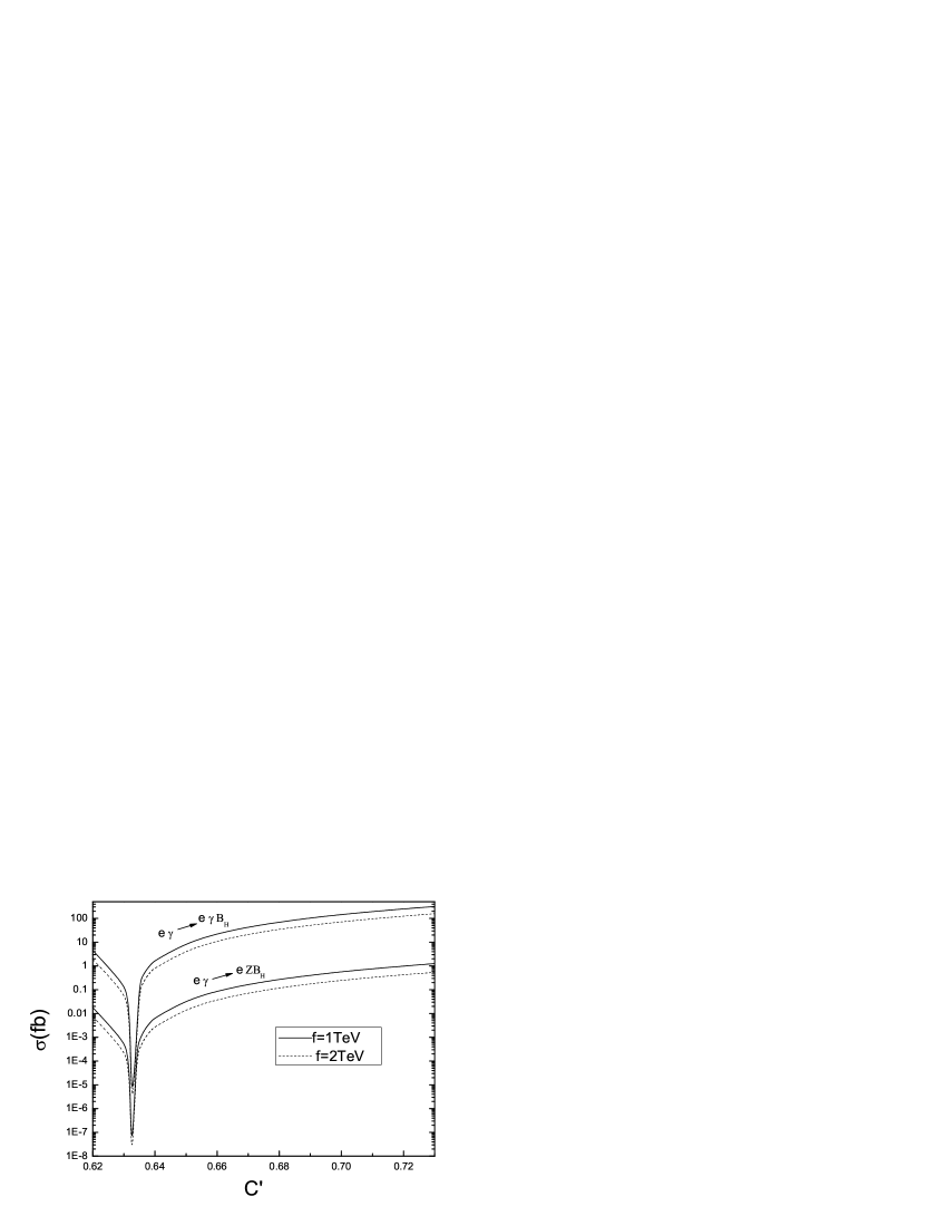
Figure 2: The production cross sections of the processes $e^{-}\gamma\rightarrow e^{-}\gamma B_{H}$ (upper curves) and $e^{-}\gamma\rightarrow e^{-}ZB_{H}$ (lower curves) as a function of the mixing parameter $c^{\prime}$ for $\sqrt{s}=800$ GeV and the scale parameter f=1 TeV(solid line), and f=2 TeV(dashed line), respectively.

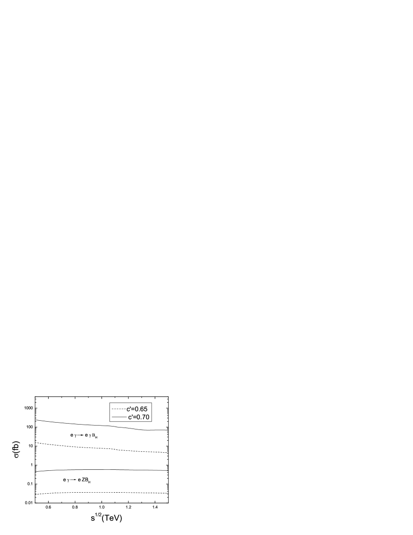
Figure 3: The production cross sections of the processes $e^{-}\gamma\rightarrow e^{-}\gamma B_{H}$(upper curves) and $e^{-}\gamma\rightarrow e^{-}ZB_{H}$(lower curves) as a function of the c.m. energy $\sqrt{s}$ for f=1 TeV and the mixing parameter c’=0.70(solid line), and c’=0.65(dashed line), respectively.

The production cross sections of the processes $e^{-}\gamma\rightarrow e^{-}\gamma B_{H}$ and $e^{-}\gamma\rightarrow e^{-}ZB_{H}$ are not sensitive to c, and we fix the value of c as 0.4 in our calculation. The cross sections mainly depend on the mixing parameter $c^{\prime}$. So in Fig.2 we plot the cross sections as a function of the parameter $c^{\prime}$, taking $\sqrt{s}=0.8$ TeV and f=1 TeV(2 TeV) as the examples. From Fig.2, one can see that the cross sections drop sharply to zero when $c^{\prime}$ equals $\sqrt{2/5}$. This is because the coupling of the gauge boson $B_{H}$ to the electron pair become decoupled with $c^{\prime}=\sqrt{2/5}$. When $c^{\prime}$ is over $\sqrt{2/5}$, the cross sections increase with $c^{\prime}$ and the cross section of the process $e^{-}\gamma\rightarrow e^{-}\gamma B_{H}$ can reach the level of tens fb even a hundred fb. But the cross section of the process $e^{-}\gamma\rightarrow e^{-}ZB_{H}$ is much smaller than that of $e^{-}\gamma\rightarrow e^{-}\gamma B_{H}$ and its maximum can only reach the level of 1 fb. So the process $e^{-}\gamma\rightarrow e^{-}\gamma B_{H}$ should have advantage in probing $B_{H}$. On the other hand, comparing the results for f=1 TeV with those for f=2 TeV, we find that the cross sections decrease slightly with f increasing. This is mainly because that the mass of $B_{H}$ increases with f increasing which can depress the phase space.

To show the influence of the c.m. energy $\sqrt{s}$ on the cross sections, we plot the cross sections as a function of $\sqrt{s}$ with f=1 TeV and $c^{\prime}=0.65,0.70$ in Fig.3. Considering the c.m. energy at the ILC and the kinetic limit, we present the numerical results for energies ranging from 0.5 to 1.5 TeV. The results show that the cross section of $e^{-}\gamma B_{H}$ production slightly decreases with $\sqrt{s}$ and the cross section of $e^{-}ZB_{H}$ production is more insensitive to $\sqrt{s}$.

The yearly luminosity of the ILC can reach $500fb^{-1}$. So we can conclude that the sufficient typical $B_{H}$ events can be produced via $e\gamma$ collision, specially via the process $e^{-}\gamma\rightarrow e^{-}\gamma B_{H}$. But to detect $B_{H}$, one also needs to study the decay modes of $B_{H}$ which has been done in reference[12]. The decay width of a particle affects how and to what extent it is experimentally detectable, since production of particles with very large decay widths may be difficult to distinguish from background processes. For $B_{H}$, the parameter spaces where the large decay width would occur are beyond current search limits in any case. So if $B_{H}$ would be produced it can be detected via the measurement of the peak in the invariant mass distribution of its decaying particles. On the other hand, for the process $e^{-}\gamma\rightarrow e^{-}\gamma B_{H}$, the backgrounds are likely to be more larger in the collision direction because it is difficult to distinguish the final state $e^{-}\gamma$ from the injecting $e^{-}\gamma$. But the backgrounds can be significantly depressed if the detection is taken in the direction of deviating the collision.

In the following, we focus on discussing how to detect $B_{H}$ via its decay modes. The main decay modes of $B_{H}$ are $e^{+}e^{-}+\mu^{+}\mu^{-}+\tau^{+}\tau^{-},~{}d\bar{d}+s\bar{s},~{}u\bar{u}+c\bar{c},~{}ZH,~{}W^{+}W^{-}$. The decay branching ratios of these modes have been studied in reference[12] which are strongly dependent on the $U(1)$ charge assignments of the SM fermions. In general, the heavy gauge bosons are likely to be discovered via their decays modes to leptons. For $B_{H}$, the most interesting decay modes should be $e^{+}e^{-},~{}\mu^{+}\mu^{-}$. This is because such leptons can be easily identified and the number of $e^{+}e^{-},~{}\mu^{+}\mu^{-}$ background events with such a high invariant mass is very small. So, the measurement of the peak in the invariant mass distribution of $e^{+}e^{-},~{}\mu^{+}\mu^{-}$ can provide a unique way to probe $B_{H}$. For the signal $e^{-}\gamma e^{+}e^{-}(\mu^{+}\mu^{-})$, the main SM background arises from $e^{-}\gamma\rightarrow e^{-}\gamma Z$ with $Z\rightarrow e^{+}e^{-}(\mu^{+}\mu^{-})$. The cross section is a few pb with $\sqrt{s}$ =0.5 $\sim$ 1.5 TeV [22]. For the signal $e^{-}Ze^{+}e^{-}(\mu^{+}\mu^{-})$, the most serious SM backgrounds come from the processes $e^{-}\gamma\rightarrow e^{-}ZZ$, $e^{-}\gamma\rightarrow e^{-}ZH$ and their cross sections can reach about 10 fb, a few fb, respectively, in the energy range $\sqrt{s}=0.5\sim 1.5$ TeV[23]. But one can very easily distinguish $B_{H}$ from $Z$ via their significantly different $e^{+}e^{-}$($\mu\mu$) invariant mass distribution. The backgrounds of $e^{-}\gamma\rightarrow e^{-}ZH$ with H decaying to lepton pair or light quark pair are very small because the decay branching ratios of these H decay modes are depressed by the small masses of leptons and light quarks. On the other hand, we can also distinguish $B_{H}$ from H via their different invariant mass distribution of final particles because $B_{H}$ is much heavier than H. As we know, in a narrow region around $c^{\prime}=0.63$, the decay branching ratios of $B_{H}\rightarrow l^{+}l^{-}$ approach zero due to the decoupling of $B_{H}$ with lepton pair. In this case, the main decay modes of $B_{H}$ are $B_{H}\rightarrow W^{+}W^{-},ZH$. The decay mode $Z\rightarrow W^{+}W^{-}$ is of course kinematically forbidden in the SM but $H\rightarrow W^{+}W^{-}$ is the dominant decay mode with Higgs mass above 135 GeV(one or both of W is off-shell for Higgs mass below 2$M_{W}$). So the background for the signal $e^{-}ZW^{+}W^{-}$ might be serious and it is hard to detect the $B_{H}$ via $e^{-}\gamma\rightarrow e^{-}ZB_{H}$ with $B_{H}\rightarrow W^{+}W^{-}$. However, the process $e^{-}\gamma\rightarrow e^{-}\gamma B_{H}$ does not suffer such large background problem which would be another advantage of $e^{-}\gamma\rightarrow e^{-}\gamma B_{H}$. For $B_{H}\rightarrow ZH$, the main final states are $l^{+}l^{-}b\bar{b}$. In this case, two b-jets can be reconstructed to the Higgs mass and a $l^{+}l^{-}$ can be reconstructed to the Z mass and the background is very clean. Furthermore, the decay mode $ZH$ involves the off-diagonal coupling $HZB_{H}$ and the factor $cot2\psi^{\prime}$ in the coupling $HZB_{H}$ is a unique feature of the littlest Higgs model. It should also be mentioned that experimental precision measurement of such off-diagonal coupling is more easier than that of diagonal coupling. So, the decay mode $ZH$ would not only provide a better way to probe $B_{H}$ but also provide a robust test of the littlest Higgs model.

In conclusion, the realization of $e\gamma$ or $\gamma\gamma$ collision at the planed ILC with high energy and luminosity will provide more chances to probe the new particles predicted by the new physics beyond the SM. In this paper, we study the new gauge boson $B_{H}$ production processes via $e\gamma$ collision, i.e., $e^{-}\gamma\rightarrow e^{-}\gamma B_{H},~{}e^{-}ZB_{H}$. The study shows that the cross section of $e^{-}\gamma\rightarrow e^{-}ZB_{H}$ can reach the level of less than one fb in most parameter spaces while the cross section of the process $e^{-}\gamma\rightarrow e^{-}\gamma B_{H}$ can reach the level of tens fb and even hundreds of fb in most parameter spaces allowed by the electroweak precision data. We can predict that there are enough $B_{H}$ signals can be produced via these processes, specially via $e^{-}\gamma\rightarrow e^{-}\gamma B_{H}$ at the planned ILC. Because the new gauge boson $B_{H}$ can be easily distinguished from the SM Z and H, the signal would be typical and the background would be very clean. So, the processes $e^{-}\gamma\rightarrow e^{-}\gamma B_{H},~{}e^{-}ZB_{H}$ will provide a good chance to probe $B_{H}$ and test the littlest Higgs model.

References

• [1] For a recent review see: M. Schmaltz and D. Tucker-Smith, Ann. Rev. Nucl. Part. Sci. 55, 229(2005); T. Han, H. E. Logen, B. McElrath and L. T. Wang, JHEP 0601, 099(2006).
• [2] N. Arkani-Hamed, A. G. Cohen, T. Gregoire, and J. G. Wacker, JHEP 0208, 020(2002); N. Arkani-Hamed, A. G. Cohen, E. Katz, A. E. Nelson, T. Gregoire, and J. G. Wacker, JHEP 0208, 021(2002).
• [3] I. Low, W. Skiba, and D. Smith, Phys. Rev. D66, 072001(2002); W. Skiba and J. Terning, Phys. Rev. D68, 075001(2003); D. E. Kaplan and M. Schmaltz, JHEP 0310, 039(2003).
• [4] S. Chang and J. G. Wacker, Phys.Rev. D69, 035002(2004); S. Chang, JHEP 0312, 057(2003).
• [5] N. Arkani-Hamed, A. G. Cohen, E. Katz, A. E. Nelson, JHEP 0207 034(2002).
• [6] For recent review see: M. Perelstein, Prog. Part. Nucl. Phys. 58, 247(2007).
• [7] B. Badelek et.al., The Photon Collider at TESLA, Inter. Jour. Mod. Phys. A30, 5097(2004).
• [8] V. I. Thlnov, Acta Phys. Polon. B37, 1049(2006); V. I. Telnov, Acta Phys. Polon. B37, 633(2006); M. Battaglia, T. Barklow, M. E. Peskin, Y. Okada, S. Yamashita, P. Zerwas, hep-ex/0603010.
• [9] E. Boos et al., Nucl.Instrum. Methods Phys.Res.,Sect. A472, 100(2001); S. J. Brodsky, Int. J. Mod. Phys. A18, 2871(2003).
• [10] X. L. Wang, J. H. Chen, Y. B. Liu, S. Z. Liu, H. Yang, Phys. Rev. D74, 015006(2006).
• [11] C. X. Yue and W. Wang, Phys.Rev. D71, 015002(2005).
• [12] T. Han, H. E. Logan, B. McElrath, and L. T. Wang, Phys. Rev. D67, 095004(2003).
• [13] H. E. Logan, Phys.Rev. D70, 115003 (2004).
• [14] A. J. Buras, A. Poschenrieder and S. Uhlig, Nucl.Phys. B716, 173(2005); S. R. Choudhury, N. Gaur, G. C. Joshi and B. H. J. McKellar, hep-ph/0408125; S. R. Choudhury, N. Gaur, A. Goyal and N.Mahajan, Phys.Lett. B601, 164(2004).
• [15] S. C. Park, J. Song, Phys. Rev. D69, 115010(2004); J. Hubisz and P. Meade, Phys.Rev. D71, 035016(2005); M. Schmaltz and D. Tucker-Smith, Ann.Rev.Nucl.Part.Sci. 55, 229(2005); W.Kilian and J. Reuter, Phys.Rev. D 70, 015004 (2004); M. Blanke, A.J. Buras, A.poschenrieder, S. Recksiegel, C. Tarantino, S. Uhlig, and A. Weiler, JHEP 0701, 066(2007); M. C. Chen and S. Dawson, Phys.Rev. D70, 015003(2004); M. C. Chen, Mod.Phys.Lett. A21, 621(2006); R. Casalbuoni, A. Deandrea and M.Oertel, JHEP 0402, 032(2004).
• [16] J. A. Conley, J. Hewett, and M. P. Le, Phys. Rev. D72, 115014(2005).
• [17] J. L. Hewett, F. J. Petriello, and T. G. Rizzo, JHEP 0310, 062(2003); C. Csaki, J. Hubisz, G. D. Kribs, P. Meade, and J. Terning, Phys.Rev. D67, 115002(2003).
• [18] C. Csaki, J. Hubisz, G. D. Kribs, P. Meade, and J. Terning, Phys.Rev. D68, 035009(2003); T. Gregoire, D. R. Smith and J. G. Wacker, Phys.Rev. D69, 115008(2004).
• [19] A. J. Buras, A. Poschenrieder, S. Uhlig, and W. A. Bardeen, JHEP 0611, 062(2006).
• [20] G. Jikia, Nucl. Phys. B374, 83(1992); O. J. P. Eboli, etΒ al., Phys. Rev. D47, 1889(1993); K. M. Cheung, ibid. 47, 3750(1993).
• [21] J. F. Donoghue, E. Golowich, and B. R. Holstein, Dynamics of the Standard Model, Cambridge Univiversity Press, 1992, P. 34.
• [22] S. Dittmaier and M. B$\ddot{o}$hm, Nucl.Phys. B412, 39(1994).
• [23] O. J. P.Eboli, M. C. Gonzal$\acute{e}$z-Garc$\acute{l}$a, and S. F. Novaes, Nucl. Phys. B411, 381(1994); K. Cheung, Nucl. Phys. B403, 572(1993).