QCD effective action with a most general homogeneous field background

Abstract

We consider one-loop effective action of $SU(3)$ QCD with a most general constant chromomagnetic (chromoelectric) background which has two independent Abelian field components. The effective potential with a pure magnetic background has a local minimum only when two Abelian components $H_{\mu\nu}^{3}$ and $H_{\mu\nu}^{8}$ of color magnetic field are orthogonal to each other. The non-trivial structure of the effective action has important implication in estimating quark-gluon production rate and $p_{T}$-distribution in quark-gluon plasma. In general the production rate depends on three independent Casimir invariants, in particular, it depends on the relative orientation between chromoelectric fields.

1. Introduction

An interesting problem which has been studied recently is to calculate the soft gluon production rate in a constant chromoelectric background cash ; nayak . This problem arises when one wishes to find the gluon production rate in quark-gluon plasma produced in high energy hadron collider experiments exp . One faces the same problem when one wants to estimate the decay rate of a chromoelectric knot which might exist in QCD chopl . This problem is closely related to the problem to calculate the QCD effective action in a constant chromoelectric background since the imaginary part of the effective action determines the production rate schw . There have been considerable amount of discussions on this problem in the literature savv ; yil ; sch ; ambj1 ; ditt ; flyv ; avr ; prd02 ; cho99 .

In the present Letter we calculate one-loop QCD effective action in most general homogeneous chromomagnetic and chromoelectric external fields. The generic structure of $SU(3)$ QCD effective action is not much different from that of $SU(2)$ QCD. A new feature is that $SU(3)$ Lie algebra has rank two due to the Cartan subalgebra $U(1)\times U(1)$. This implies that the most general homogeneous chromomagnetic (or chromoelectric) field contains two independent vector fields directed along two Abelian directions in the internal color space, or equivalently, along two directions in the configuration space. This leads to a more non-trivial structure of the effective action with a most general constant background, and that is what should be taken into account when solving some physical problems. Specifically, the real part of the effective potential for a constant color magnetic background has a local minimum only when two background chromomagnetic vector fields are orthogonal to each other. This unexpected and surprising result had been obtained first by Flyvbjerg flyv who suggested an improvement of the Copenhagen vacuum. Another implication is that the quark-gluon production rate in a most general chromoelectric external background depends on the angle between two independent chromoelectric vector fields. That means the quark-gluon production rate depends on three Casimir invariants in general.

2. Effective action

We consider a constant field background which can be defined in an appropriate gauge by only Abelian gauge components $A_{\mu}^{i}~{}(i=3,8)$ corresponding to the Cartan algebra of $SU(3)$. To calculate the effective action we integrate out the off-diagonal (valence) gluons $X_{\mu}^{a}$ from the generating functional of one-point irreducible Green functions. For this it is convenient to introduce three complex vector fields ($W_{\mu}^{p},~{}p=1,2,3$ )

$$W^{1}_{\mu}=\displaystyle\frac{1}{\sqrt{2}}(X_{\mu}^{1}+iX_{\mu}^{2}),~{}~{}~{}~{}~{}W^{2}_{\mu}=\displaystyle\frac{1}{\sqrt{2}}(X_{\mu}^{6}+iX_{\mu}^{7}),~{}~{}~{}~{}~{}W^{3}_{\mu}=\displaystyle\frac{1}{\sqrt{2}}(X_{\mu}^{4}-iX_{\mu}^{5}).$$ (1)

This allows us to express a pure QCD Lagrangian in an explicitly Weyl invariant form

$${\cal L}=-\displaystyle\frac{1}{4}\vec{F}_{\mu\nu}^{2}=\sum_{p}\Big{\{}-\displaystyle\frac{1}{6}({\cal G}_{\mu\nu}^{p})^{2}+\displaystyle\frac{1}{2}|D_{p\mu}W_{\nu}^{p}-D_{p\nu}W_{\mu}^{p}|^{2}-ig{\cal G}_{\mu\nu}^{p}W_{\mu}^{p*}W_{\nu}^{p}-\displaystyle\frac{1}{2}g^{2}\big{[}(W_{\mu}^{p*}W_{\mu}^{p})^{2}-(W_{\mu}^{p*})^{2}(W_{\nu}^{p})^{2}\big{]}\Big{\}},$$

$${\cal G}_{\mu\nu}^{p}=\partial_{\mu}{\cal B}_{\nu}^{p}-\partial_{\nu}{\cal B}_{\mu}^{p},~{}~{}~{}~{}~{}~{}D_{p\mu}W_{\nu}^{p}=(\partial_{\mu}-ig{\cal B}_{\mu}^{p})W_{\nu}^{p},~{}~{}~{}~{}~{}~{}{\cal B}_{\mu}^{p}=A_{\mu}^{i}{\vec{r}}_{i}^{\,p},$$ (2)

where the $SU(3)$ root vectors ${\vec{r}}_{p}$ are given by

$${\vec{r}}_{i}^{\,1}=(1,0),~{}~{}~{}~{}{\vec{r}}_{i}^{\,2}=(-1/2,\sqrt{3}/2),~{}~{}~{}~{}{\vec{r}}_{i}^{\,3}=(-1/2,-\sqrt{3}/2).$$ (3)

Notice that the Abelian background fields ${\cal B}_{\mu}^{p}$ are precisely the dual potentials in $i$-spin, $u$-spin, and $v$-spin direction in color space which couple to three valence gluons $W_{\mu}^{p}$. With this we have the following functional integral form of the one-loop effective action

$$\exp\Big{[}iS_{eff}(A_{\mu})\Big{]}=\displaystyle\frac{}{}\sum_{p}\int{\cal D}(W_{\mu},c_{1},c_{2})\exp\Big{\{}\displaystyle\frac{}{}i\int\Big{[}-\displaystyle\frac{1}{6}{\cal G}_{\mu\nu}^{2}+\displaystyle\frac{1}{2}|{D}_{\mu}{W}_{\nu}-{D}_{\nu}{W}_{\mu}|^{2}$$

$$-ig{\cal G}_{\mu\nu}W_{\mu}^{*}W_{\nu}-\displaystyle\frac{1}{2}g^{2}\Big{[}(W_{\mu}^{*}W_{\mu})^{2}-(W_{\mu}^{*})^{2}(W_{\nu})^{2}\Big{]}-\displaystyle\frac{1}{\xi}|{D}_{\mu}W_{\mu}|^{2}$$

$$+c_{1}^{\dagger}({D}^{2}+g^{2}W_{\mu}^{*}W_{\mu})c_{1}-g^{2}c_{1}^{\dagger}W_{\mu}W_{\mu}c_{2}+c_{2}^{\dagger}({D}^{2}+g^{2}W_{\mu}^{*}W_{\mu})^{*}c_{2}-g^{2}c_{2}^{\dagger}W^{*}_{\mu}W^{*}_{\mu}c_{1}~{}\Big{]}d^{4}x\Big{\}},$$ (4)

where $\xi$ is a gauge fixing parameter and $c_{1,2}$ are the ghost fields, and here we have suppressed the summation index $p$ in the integrand. Now a few remarks are in order. First, notice that except for the $p$-summation the integral expression is identical to that of $SU(2)$ QCD prd02 . This shows that one can reduce the calculation of QCD effective action to that of $SU(2)$ QCD. Secondly, the above result can easily be generalized to $SU(N)$ QCD with $N(N-1)/2$ $p$-summation. Thirdly, one might include the Abelian part in the functional integration, but this does not affect the result because the Abelian part has no self-interaction. This tells that only the valence gluon loops contribute to the integration.

Now, in the same manner as in $SU(2)$ QCD prd02 we can derive the functional determinant form for the one-loop correction $\Delta S$ to the effective action (with $\xi=1/2$)

$$\Delta S = i\sum\limits_{p}\ln{\rm Det}[(-D_{p}^{2}+2gH_{p})(-D_{p}^{2}-2gH_{p})]+i\sum\limits_{p}\ln{\rm Det}[(-D_{p}^{2}-2igE_{p})(-D_{p}^{2}+2igE_{p})]$$

$$-2i\sum_{p}\ln{\rm Det}[-D_{p}^{2}],$$

$$H_{p} = \displaystyle\frac{1}{2}\sqrt{\sqrt{{\cal G}_{p}^{4}+({\cal G}_{p}\tilde{\cal G}_{p})^{2}}+{\cal G}_{p}^{2}},~{}~{}~{}~{}~{}~{}E_{p}=\displaystyle\frac{1}{2}\sqrt{\sqrt{{\cal G}_{p}^{4}+({\cal G}_{p}\tilde{\cal G}_{p})^{2}}-{\cal G}_{p}^{2}},~{}~{}~{}~{}~{}~{}\tilde{\cal G}_{\mu\nu}=\displaystyle\frac{1}{2}\epsilon_{\mu\nu\rho\sigma}{\cal G}^{\rho\sigma},$$ (5)

from which with Schwinger’s proper time method we obtain

$$\Delta{\cal L}=\lim\limits_{\epsilon\rightarrow 0}\displaystyle\frac{g^{2}}{16\pi^{2}}\sum_{p}\int_{0}^{\infty}\displaystyle\frac{dt}{t^{1-\epsilon}}\displaystyle\frac{H_{p}E_{p}}{\sinh(gH_{p}t/\mu^{2})\sin(gE_{p}t/\mu^{2})}\Big{[}\exp(-2gH_{p}t/\mu^{2})+\exp(+2gH_{p}t/\mu^{2})$$

$$+\exp(+2igE_{p}t/\mu^{2})+\exp(-2igE_{p}t/\mu^{2})-2\Big{]},$$ (6)

where $\mu$ is a mass parameter. One should emphasize that the expression (5) is valid for arbitrary magnetic and electric fields, whereas the integral representation (6) is applicable only to constant field configurations. Notice also that the integral representation is intrinsically ill-defined and has ambiguity due to the pole structure. Moreover, it contains a well-known infra-red divergence which has to be regularized. The mathematical ambiguity in (6) reflects the existence of different physical problems to which the constant field approximation has been applied.

The case of general electric-magnetic background of $SU(3)$ QCD is in full analogy with the corresponding case of $SU(2)$ QCD. The analytical expression for the effective action of $SU(2)$ QCD with a general electric-magnetic constant background has been obtained in cho99 . So that we will consider only two special cases of pure magnetic and pure electric external field concentrating on features of the $SU(3)$ structure of QCD.

Let us consider first the constant chromomagnetic external field. The corresponding effective Lagrangian of $SU(2)$ QCD including both, the real and imaginary parts, had been calculated in the well-known paper by Nielsen and Olesen savv . The corresponding expression for $SU(3)$ QCD has the same structure

$${\cal L}_{eff} = -\sum\limits_{p}\Big{(}\displaystyle\frac{H_{p}^{2}}{3}+\displaystyle\frac{11g^{2}}{48\pi^{2}}H_{p}^{2}(\ln\displaystyle\frac{gH_{p}}{\mu^{2}}-c)+\displaystyle\frac{ig^{2}}{8\pi}H_{p}^{2}\Big{)},$$ (7)

where $c=1.2921...$ (within the modified minimal subtraction scheme). The Lagrangian has an imaginary part which implies the existence of a tachyonic mode in the theory and instability of the constant external chromomagnetic field.

The effective Lagrangian possesses a manifest Weyl symmetry provided by the six-element subgroup of $SU(3)$ which contains the cyclic group $Z_{3}$. We can also express the effective Lagrangian (7) in terms of three Casimir invariants

$$C_{2}=\displaystyle\frac{1}{2}(F_{\mu\nu}^{i})^{2},~{}~{}~{}~{}C_{4}=(d^{ijk}F_{\mu\nu}^{j}F_{\mu\nu}^{k})^{2},~{}~{}~{}~{}C_{6}=(d^{ijk}F_{\mu\nu}^{i}F_{\nu\rho}^{j}F_{\rho\sigma}^{k})^{2}.$$ (8)

One can check that $H_{p}$ satisfy the equations:

$$H_{1}^{2}+H_{2}^{2}+H_{3}^{2}=3C_{2}\equiv\alpha,$$

$$H_{1}^{2}H_{2}^{2}+H_{2}^{2}H_{3}^{2}+H_{3}^{2}H_{1}^{2}=3C_{2}^{2}-\displaystyle\frac{9}{16}C_{4}\equiv\beta,$$

$$H_{1}^{2}H_{2}^{2}H_{3}^{2}=C_{2}^{3}-\displaystyle\frac{3}{8}C_{2}C_{4}-\displaystyle\frac{3}{2}C_{6}\equiv\gamma,$$ (9)

where we denote for a convenience the right hand sides of the equations by $\alpha,\beta,\gamma$ respectively.

We generalize the equations for $H_{p}$ (9) by assuming that arbitrary constant magnetic background fields $H_{p}$ satisfy the same equations, so that $H_{p}^{2}$ are represented by real roots of the cubic equation

$$x^{3}-\alpha x^{2}+\beta x-\gamma=0.$$ (10)

The solution to the equation provides the values of $H_{p}$ in terms of Casimir invariants

$$H_{p}^{2}=\displaystyle\frac{\sqrt{3C_{4}}}{2}\sin\phi_{p}+C_{2},$$ (11)

where $\phi_{p}$ are three basic solutions of the equation ($[0\leq\phi\leq 2\pi]$)

$$\sin 3\phi=\displaystyle\frac{2}{\sqrt{3}}\displaystyle\frac{(8C_{6}-C_{2}C_{4})}{C_{4}^{3/2}}.$$ (12)

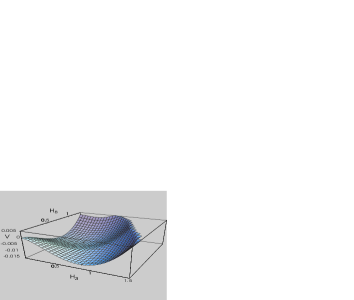
Figure 1: The QCD effective potential with $\cos\theta=1$, which has two degenerate minima ($c=5/4$).

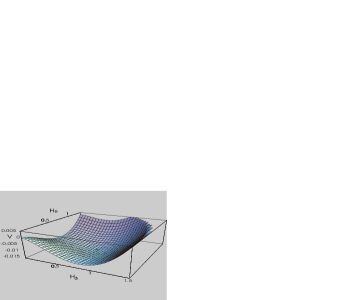
Figure 2: The effective potential with $\cos\theta=0$, which has a unique minimum at $\bar{H}_{3}=\bar{H}_{8}=H_{0}$  ($c=5/4$).

Just as in $SU(2)$ QCD we can obtain the effective potential from the effective action. For the constant magnetic background a real part of the effective potential is given by

$$V_{eff} = \displaystyle\frac{1}{2}(\bar{H}_{3}^{2}+\bar{H}_{8}^{2})+\displaystyle\frac{11g^{2}}{48\pi^{2}}\Big{\{}\bar{H}_{3}^{2}\big{(}\ln\displaystyle\frac{g\bar{H}_{3}}{\mu^{2}}-c\big{)}+\bar{H}_{+}^{2}\big{(}\ln\displaystyle\frac{g\bar{H}_{+}}{\mu^{2}}-c\big{)}+\bar{H}_{-}^{2}\big{(}\ln\displaystyle\frac{g\bar{H}_{-}}{\mu^{2}}-c\big{)}\Big{\}},$$

$$\bar{H}_{\pm}^{2} = \displaystyle\frac{1}{4}\bar{H}_{3}^{2}+\displaystyle\frac{3}{4}\bar{H}_{8}^{2}\pm\displaystyle\frac{\sqrt{3}}{2}\bar{H}_{3}\bar{H}_{8}\cos\theta,$$

$$\bar{H}_{3} = \sqrt{(H_{\mu\nu}^{3})^{2}/2},~{}~{}~{}\bar{H}_{8}=\sqrt{(H_{\mu\nu}^{8})^{2}/2},~{}~{}~{}~{}\cos\theta=H_{\mu\nu}^{3}H_{\mu\nu}^{8}/2\bar{H}_{3}\bar{H}_{8}.$$ (13)

Notice that the classical potential depends only on $\bar{H}_{3}^{2}+\bar{H}_{8}^{2}$, but the effective potential depends on three variables $\bar{H}_{3}$, $\bar{H}_{8}$, and $\cos\theta$. We emphasize that $\cos\theta$ can be arbitrary because $H_{\mu\nu}^{3}$ and $H_{\mu\nu}^{8}$ are completely independent, so that they can have different space polarization.

When $H_{\mu\nu}^{3}$ and $H_{\mu\nu}^{8}$ are parallel ($\cos\theta=1$) it has two degenerate minima at $\bar{H}_{3}=2^{1/3}H_{0},~{}\bar{H}_{8}=0$ and at $\bar{H}_{3}=2^{-2/3}H_{0},~{}\bar{H}_{8}=2^{-2/3}\sqrt{3}H_{0}$. When $\theta$ approaches the value $\pm\pi/2$ the two minima merge into one minimum at $\bar{H}_{3}=\bar{H}_{8}=H_{0}$

$$H_{0}=\displaystyle\frac{\mu^{2}}{g}\exp\big{(}-\displaystyle\frac{16\pi^{2}}{11g^{2}}+c-\displaystyle\frac{1}{2}\big{)}.$$ (14)

We plot the effective potential for $\cos\theta=1$ in Fig. 1 and for $\cos\theta=0$ in Fig. 2 for comparison.

Usually, in most physical applications, the constant background field is chosen to be directed along one direction in the configuration (or internal) space by imposing the constraint $\cos\theta=1$. Our analysis shows that if we start with such a special background we would never reach the absolute minimum of the effective potential. This non-trivial feature of the energy functional for a pure QCD had been found first in flyv . Notice also that this minimum represents a saddle point in the space of all possible non-constant chromomagnetic fields due to the presence of the Nielsen-Olesen imaginary part. So that it does not correspond to a true stable vacuum. A possible stable vacuum, so-called ”Copenhagen vacuum”, has been proposed in niel2 ; ambj3 . An interesting example of a stable solution made of a pair of monopole-antimonopole strings in $SU(2)$ QCD has been obtained recently in cho11 .

One can renormalize the potential by defining a running coupling $\bar{g}^{2}(\bar{\mu}^{2})$

$$\displaystyle\frac{\partial^{2}V_{eff}}{\partial\bar{H}_{i}^{2}}\Big{|}_{\bar{H}_{3}=\bar{H}_{8}=\bar{\mu}^{2},\theta=\pi/2}=\displaystyle\frac{g^{2}}{\bar{g}^{2}},$$ (15)

from which we can retrieve the correct QCD $\beta$-function. The renormalized potential has the same form as in (13), with the formal replacement $g\rightarrow\bar{g},~{}\mu\rightarrow\bar{\mu},~{}c=5/4$. It has the unique absolute minimum

$$V_{min}=-\displaystyle\frac{11\bar{\mu}^{4}}{32\pi^{2}}\exp\big{(}-\displaystyle\frac{32\pi^{2}}{11\bar{g}^{2}}+\displaystyle\frac{3}{2}\big{)}.$$ (16)

For a constant chromoelectric field background one can obtain a similar integral expression for the one-loop contribution to the effective Lagrangian

$$\Delta{\cal L}=\displaystyle\frac{g}{16\pi^{2}}\lim\limits_{\epsilon\rightarrow 0}\sum_{p}\int_{0}^{\infty}\displaystyle\frac{dt}{t^{2-\epsilon}}\displaystyle\frac{E_{p}}{\sin(gE_{p}t)}\Big{(}\exp(+2igE_{p}t)+\exp(-2igE_{p}t)\Big{)}.$$ (17)

The chromoelectric fields $E_{p}$ can be expressed in terms of corresponding Casimir invariants by an equation similar to (11). In a special case, when two background chromoelectric fields $F_{\mu\nu i}$ lie along one direction in the color space, the Casimir invariant $C_{4}$ is not longer independent and can be expressed in terms of lower Casimir $C_{2}$. With this the general solution for $E_{p}$ is simplified to a special one obtained recently in nayak .

3. Quark production rate

The quark contribution to the effective action of QCD does not have strong infra-red divergency problem, and its calculation is straightforward as in $SU(2)$ theory. The Lagrangian of $SU(3)$ QCD with quarks interacting with the Abelianized gauge potential can be written as follows

$${\cal L}_{q}=-\displaystyle\frac{1}{8}\sum_{p}({\cal F}_{\mu\nu}^{p})^{2}+\sum_{p}\bar{\Psi}_{p}(i\gamma^{\mu}{\cal D}_{p\mu}-m)\Psi_{p},$$

$${\cal F}_{\mu\nu}^{p}=\partial_{\mu}{\cal A}_{\nu}^{p}-\partial_{\nu}{\cal A}_{\mu}^{p},~{}~{}~{}~{}{\cal D}_{p\mu}=\partial_{\mu}-i\displaystyle\frac{g}{2}{\cal A}_{\mu}^{p},~{}~{}~{}~{}{\cal A}_{\mu}^{p}=A_{\mu}^{i}\vec{w}_{i}^{\,p},$$ (18)

where $m$ is the quark mass, and $\vec{w}^{\,p}$ are weights of $SU(3)$. One can express the quark contribution to the one-loop effective action in a Weyl invariant form

$$\Delta{\cal L}_{q}=-\displaystyle\frac{g^{2}}{16\pi^{2}}\sum_{p}\int_{0}^{\infty}\displaystyle\frac{dt}{t^{1-\epsilon}}{\cal H}_{p}{\cal E}_{p}\coth(g{\cal H}_{p}t/2)\cot(g{\cal E}_{p}t/2)\exp(-m^{2}t),$$ (19)

where we introduce gauge invariant variables ${\cal H}_{p},~{}{\cal E}_{p}$ corresponding to the pure magnetic and electric fields defined as in (5). The analytical series representation for $SU(2)$ QCD effective action with a general constant background has been obtained in cho99 , so that we will concentrate mainly on some new features appeared in $SU(3)$ theory and consider particularly the pair production in quark-gluon plasma in what follows.

Let us consider $p_{T}$-distribution of the quark production rate in constant chromoelectric background

$$\Delta{\cal L}_{q}=-\displaystyle\frac{g}{16\pi^{3}}\sum_{p}\int_{0}^{\infty}d^{2}p_{T}\displaystyle\frac{dt}{t^{1-\epsilon}}{\cal E}_{p}\cot(g{\cal E}_{p}t/2)\exp[-(p_{T}^{2}+m^{2})t],$$

$${\cal E}_{1}={\cal E}_{+},~{}~{}~{}{\cal E}_{2}={\cal E}_{-},~{}~{}~{}{\cal E}_{3}=2\bar{E}_{8}/\sqrt{3},$$

$${\cal E}_{\pm}=\sqrt{\bar{E}_{3}^{2}+\bar{E}_{8}^{2}/3\pm 2\bar{E}_{3}\bar{E}_{8}\cos\theta/\sqrt{3}},$$

$$\bar{E}_{3}=\sqrt{(F_{\mu\nu}^{3})^{2}/2},~{}~{}~{}\bar{E}_{8}=\sqrt{(F_{\mu\nu}^{8})^{2}/2},~{}~{}~{}\cos\theta=F_{\mu\nu}^{3}F_{\mu\nu}^{8}/2\bar{E}_{3}\bar{E}_{8},$$ (20)

here, $\theta$ is the angle between two chromoelectric fields $F_{\mu\nu}^{3}$ and $F_{\mu\nu}^{8}$. For the quark contribution we have no acausal states, so that the contour above the $t$-axis from $0+\epsilon$ does become the causal contour. This implies nayak

$$Im~{}\Delta{\cal L}_{q}=\displaystyle\frac{g}{16\pi^{3}}\sum_{p}\sum_{n=1}^{\infty}\displaystyle\frac{1}{n}{\cal E}_{p}\exp\Big{(}-\displaystyle\frac{2\pi n(p_{T}^{2}+m^{2})}{g{\cal E}_{p}}\Big{)}.$$ (21)

The imaginary part depends on three independent variables, $\bar{E}_{3}$, $\bar{E}_{8}$, and $\cos\theta$. One can express the imaginary part in terms of three Casimir invariants in a similar manner as in the previous section

$${\cal E}_{p}^{2} = -\sqrt{\displaystyle\frac{C_{4}}{3}}\sin\phi_{p}+\displaystyle\frac{2}{3}C_{2},$$ (22)

with values of $\phi_{p}$ given by the same Eqn. (12). A special case when $\cos\theta=1$ has been considered in nayak .

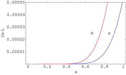
We can obtain a general expression for the total production rate from (21) with the $p_{T}$-integral,

$$Im~{}\Delta{\cal L}_{q}|_{tot}=\displaystyle\frac{g^{2}}{32\pi^{3}}\sum_{p}\sum_{n=1}^{\infty}\displaystyle\frac{{\cal E}_{p}^{2}}{n^{2}}\exp\big{(}-\displaystyle\frac{2\pi nm^{2}}{g{\cal E}_{p}}\big{)}.$$ (23)

We plot the imaginary part (23) for two values of the angle parameter $\theta$ in Fig. 3 for comparison.

Figure 3: The quark production rate: (a) in quark-gluon plasma with $\cos\theta=0$ and (b) in hadron collider with $\cos\theta=1$. Here we put $g\bar{E}_{3}=g\bar{E}_{8}=x$, and $m=1$.

The QCD effective action has been considered before with different methods savv ; yil ; sch ; ambj1 ; ditt ; flyv ; avr . Our method has the advantage that it naturally reduces the calculation of $SU(N)$ QCD effective action to that of $SU(2)$ QCD, and we provide an explicit expression for the effective action in terms of three gauge invariant Casimir quantities for the most general constant background. In most previous approaches only a special type of constant background with one vector field component has been used. Obviously, such a limitation can not provide correct results in some physical applications.

We emphasize, however, that although the quark production rate depends on three variables in general, the actual number of independent variables depends on case by case. For example, in hadron colliders two chromoelectric fluxes $F_{\mu\nu}^{3}$ and $F_{\mu\nu}^{8}$ in head-on collisions have the same direction, the beam direction, so that we have to put $\cos\theta=1$ cash ; nayak . On the other hand, for the quark-gluon plasma in the early universe or in astrophysics we should average the angle $\theta$, because two chromoelectric fluxes in such cases have no correlation in general.

Acknowledgements

One of authors (DGP) thanks Prof. N.I. Kochelev for interesting discussions. The work is supported in part by the ABRL Program of Korea Science and Engineering Foundation (R14-2003-012-01002-0).

References

(1) A. Casher, H. Neuberger, and S. Nussinov, Phys. Rev.
D20, 179 (1979).
(2) G.C. Nayak and P. van Nieuwenhuizen,
Phys.Rev. D71 125001 (2005); G.C. Nayak, Phys.Rev. D72, 125010 (2005).
(3) Y. Schutz, J. Phys. G30, S903 (2004);
L. Mclerran and M. Gyulassy, Nucl. Phys. A750, 30 (2005).
(4) Y.M. Cho, Phys. Lett. B616, 101 (2005).
(5) J. Schwinger, Phys. Rev. 82, 664 (1951).
(6) G.K. Savvidy, Phys. Lett. B71, 133 (1977);
N.K. Nielsen and P. Olesen, Nucl. Phys. B144, 376 (1978).
(7) A. Yildiz and P. Cox, Phys. Rev. D21, 1095 (1980);
M. Claudson, A. Yilditz, and P. Cox, Phys. Rev. D22, 2022 (1980).
(8) V. Schanbacher, Phys. Rev. D26, 489 (1982).
(9) J. Ambjorn and R.J. Hughes, Phys. Lett. B113, 305 (1982);
Nucl. Phys. B197, 113 (1982).
(10) W. Dittrich and M. Reuter, Phys. Lett. B128, 321, (1983);
S. Adler, Phys. Rev. D23, 2905 (1981).
(11) H. Flyvbjerg, Nucl. Phys. B176, 379 (1980).
(12) I.G. Avramidi, J. Math. Phys. 36, 1557 (1995).
(13) Y.M. Cho, H.W. Lee, and D.G. Pak,
Phys. Lett. B 525, 347 (2002); Y.M. Cho and D.G. Pak, Phys.
Rev. D65, 074027 (2002); Y.M. Cho and M.L. Walker, Mod. Phys.
Lett. A19, 2707 (2004).
(14) Y.M. Cho and D.G. Pak, in Procs. of TMU-YALE
Symp. on ”Dynamics of Gauge Fields”, 193 (Univ. Acad. Press, Tokyo,
1999), hep-th/0006051.
(15) H.B. Nielsen and M. Ninomiya,
Nucl. Phys. B156 (1979) 1;
N.K. Nielsen and P. Olesen, Nucl. Phys. B160 (1979) 380.
(16) J. Ambjorn and P. Olesen, Nucl. Phys. B170, 60 (1980);
ibid., 265.
(17) Y.M. Cho and D.G. Pak, Phys. Lett. B632, 745 (2006).