Chiral extrapolation of nucleon magnetic form factors

Abstract

The extrapolation of nucleon magnetic form factors calculated within lattice QCD is investigated within a framework based upon heavy baryon chiral effective-field theory. All one-loop graphs are considered at arbitrary momentum transfer and all octet and decuplet baryons are included in the intermediate states. Finite range regularisation is applied to improve the convergence in the quark-mass expansion. At each value of the momentum transfer ($Q^{2}$), a separate extrapolation to the physical pion mass is carried out as a function of $m_{\pi}$ alone. Because of the large values of $Q^{2}$ involved, the role of the pion form factor in the standard pion-loop integrals is also investigated. The resulting values of the form factors at the physical pion mass are compared with experimental data as a function of $Q^{2}$ and demonstrate the utility and accuracy of the chiral extrapolation methods presented herein.

I Introduction

The study of the electromagnetic properties of the nucleon is of great importance in understanding the structure of baryons — see Refs. Gao:2003ag ; Hyde-Wright:2004gh ; Arrington:2006zm ; Perdrisat:2006hj for recent reviews. The most rigorous approach to low-energy phenomena in QCD is via numerical simulations in lattice gauge theory and many physical quantities, such as baryon masses, magnetic moments, etc. Leinweber1 ; Leinweber2 ; Leinweber0 ; Leinwebernew ; Edwards:2005ym ; Boinepalli:2006xd ; QCDSF have been investigated within lattice QCD. Because of computing limitations, most of those quantities are simulated with large quark ($\pi$) masses and an extrapolation of lattice results to the physical $\pi$ mass is needed. Early lattice extrapolations considered simple polynomial functions of $\pi$ mass. However, it is now widely acknowledged that the chiral non-analytic behavior predicted by chiral perturbation theory ($\chi$PT) must be incorporated in any quark mass extrapolation function Leinweber:1993hj ; Leinweber:2001ui ; Hemmert:2002uh ; Leinweber:1999ig ; Detmold:2001jb .

$\chi$PT has been a very useful approach to the study of low momentum processes involving mesons and baryons and has been used in various studies of baryon structure. It is based on an effective Lagrangian constructed in a systematic way and consistent with all the symmetries of QCD. The first systematic discussion for the two flavor sector, i.e. the pion-nucleon system, of how to implement the ideas of chiral power counting Weinberg , was performed in Ref. Gasser . However, treating the nucleons as relativistic Dirac fields does not allow for a one-to-one correspondence between the expansion in small momenta and quark mass on the one hand and pion loops on the other. As pointed out in Ref. Jenkins , this shortcoming can be overcome if one makes use of methods borrowed from heavy quark effective field theory (HQEFT), namely to consider the baryons as extremely heavy, static sources. The relativistic or heavy baryon chiral perturbation theory has been applied to study a range of hadron properties in QCD, including nucleon magnetic moments and charge radii Durand1 ; Kubis , the nucleon sigma commutator Borasoy:1996bx ; Leinweber3 ; Procura and moments of structure functions Detmold:2001jb ; Hemmert .

Historically, most formulations of $\chi$PT are based on dimensional or infrared regularisation. However, the physical predictions of effective field theory must be regularisation scheme independent, such that other schemes are possible and may provide advantages over the traditional approach. Indeed, Donoghue $et$ $al$. Donoghue have already reported the improved convergence of properties of effective theory formulated with what they called a “long-distance regulator”. With the most detailed studies being on the extrapolation of the nucleon mass, it has been shown that the use of finite range regularisation (FRR) enables the most systematically accurate connection of $\chi$PT and lattice simulation results Leinweber3 ; Leinweber4 ; Young2 ; Armour:2005mk ; Allton:2005fb .

The FRR $\chi$PT has been applied to the extrapolation of proton magnetic moment with the leading non-analytic contribution of pions Young:2004tb . It was found that the smooth behavior of the lattice data, together with the series truncations of the FRR expansion indicate that although higher order terms of DR can be individually large they effectively sum to zero in the region of interest. FRR $\chi$PT provides a resummation of the chiral expansion that ensures that the slow variation of magnetic moments observed in lattice QCD arises naturally in the FRR expansion. It was also predicted that the quenched and physical magnetic moments are in good agreement over a large range of pion mass, especially at large $m_{\pi}$ Young:2004tb .

In this paper, we will extrapolate the proton and neutron magnetic moments, as well as the form factors at finite momentum transfer, within a framework based upon heavy baryon chiral perturbation theory. Many methods have been used to compute the form factors at the physical value of the pion mass, including the early relativistic approach Jenkins , heavy baryon chiral perturbation theory Bernard:1992qa , the so-called small scale expansion Bernard:1998gv , relativistic chiral perturbation theory Kubis ; Fuchs:2003ir , etc.. The spectral functions of the form factors have also been investigated by calculating the imaginary parts of the form factors Bernard:1996cc ; Kaiser:2003qp . The disappointing observation was that a satisfactory description of the electromagnetic form factors was achieved only up to $Q^{2}\sim 0.1$ GeV². In order to improve this situation it is natural to consider higher order terms in chiral perturbation theory but eventually the series must diverge. In fact, effectively resumming the series by including vector meson degrees of freedom led to a satisfactory description of the electromagnetic form factors up to $Q^{2}\sim 0.4$ GeV² Kubis ; Schindler:2005ke . It is of interest to calculate the form factors at relatively large momentum transfer and pion mass because there are many experimental data in this region and it is a priority for lattice QCD to understand that data.

Because the values of the momentum transfer are quite large, it is not possible to make a systematic expansion in both $Q^{2}$ and $m_{\pi}$. Instead, we extrapolate as a function of $m_{\pi}$ at each separate value of $Q^{2}$. All the one loop contributions, including baryon octet and decuplet intermediate states, are considered. The quenched lattice data at large quark mass are used in the extrapolation, using the finding that the difference between quenched and full QCD data is usually quite small at large values of the pion mass. While this is a reasonable approach until high quality full QCD data is available (for first dynamical studies see Refs. Alexandrou:2006ru ; Gockeler:2006ui ; Edwards:2006qx ), it does mean that in comparing with experiment we must remember that there is an unknown systematic error associated with the use of quenched data. So too, we have not had lattice data available which would permit an extrapolation to the continuum ($a\rightarrow 0$) and infinite volume limits. In spite of all these caveats the results of this exploratory study are really very promising.

II Chiral Perturbation Theory

There are many papers which deal with heavy baryon chiral perturbation theory – for details see, for example, Refs. Jenkins2 ; Labrenz ; Durand2 ; Tiburzi:2004mv . For completeness, we briefly introduce the formalism in this section. In the heavy baryon chiral perturbation theory, the lowest chiral Lagrangian for the baryon-meson interaction which will be used in the calculation of the nucleon magnetic moments, including the octet and decuplet baryons, is expressed as

$${\cal L}_{v} = i{\rm Tr}\bar{B}_{v}(v\cdot{\cal D})B_{v}+2D{\rm Tr}\bar{B}_{v}S_{v}^{\mu}\{A_{\mu},B_{v}\}+2F{\rm Tr}\bar{B}_{v}S_{v}^{\mu}[A_{\mu},B_{v}]$$ (1)

$$-i\bar{T}_{v}^{\mu}(v\cdot{\cal D})T_{v\mu}+{\cal C}(\bar{T}_{v}^{\mu}A_{\mu}B_{v}+\bar{B}_{v}A_{\mu}T_{v}^{\mu}),$$

where $S_{\mu}$ is the covariant spin-operator defined as

$$S_{v}^{\mu}=\frac{i}{2}\gamma^{5}\sigma^{\mu\nu}v_{\nu}.$$ (2)

Here, $v^{\nu}$ is the nucleon four velocity (in the rest frame, we have $v^{\nu}=(1,0)$). D, F and $\cal C$ are the coupling constants. The chiral covariant derivative $D_{\mu}$ is written as $D_{\mu}B_{v}=\partial_{\mu}B_{v}+[V_{\mu},B_{v}]$. The pseudoscalar meson octet couples to the baryon field through the vector and axial vector combinations

$$V_{\mu}=\frac{1}{2}(\zeta\partial_{\mu}\zeta^{\dagger}+\zeta^{\dagger}\partial_{\mu}\zeta),~{}~{}~{}~{}~{}~{}A_{\mu}=\frac{1}{2}(\zeta\partial_{\mu}\zeta^{\dagger}-\zeta^{\dagger}\partial_{\mu}\zeta),$$ (3)

where

$$\zeta=e^{i\phi/f},~{}~{}~{}~{}~{}~{}f=93~{}{\rm MeV}.$$ (4)

The matrix of pseudoscalar fields $\phi$ is expressed as

$$\phi=\frac{1}{\sqrt{2}}\left(\begin{array}[]{lcr}\frac{1}{\sqrt{2}}\pi^{0}+\frac{1}{\sqrt{6}}\eta&\pi^{+}&K^{+}\\ \pi^{-}&-\frac{1}{\sqrt{2}}\pi^{0}+\frac{1}{\sqrt{6}}\eta&K^{0}\\ K^{-}&\bar{K}^{0}&-\frac{2}{\sqrt{6}}\eta\end{array}\right).$$ (8)

$B_{v}$ and $T^{\mu}_{v}$ are the velocity dependent new fields which are related to the original baryon octet and decuplet fields $B$ and $T^{\mu}$ by

$$B_{v}(x)=e^{im_{N}\not vv_{\mu}x^{\mu}}B(x),$$ (9)

$$T^{\mu}_{v}(x)=e^{im_{N}\not vv_{\mu}x^{\mu}}T^{\mu}(x).$$ (10)

In the chiral $SU(3)$ limit, the octet baryons will have the same mass $m_{B}$. In our calculation, we use the physical masses for baryon octets and decuplets. The explicit form of the baryon octet is written as

$$B=\left(\begin{array}[]{lcr}\frac{1}{\sqrt{2}}\Sigma^{0}+\frac{1}{\sqrt{6}}\Lambda&\Sigma^{+}&p\\ \Sigma^{-}&-\frac{1}{\sqrt{2}}\Sigma^{0}+\frac{1}{\sqrt{6}}\Lambda&n\\ \Xi^{-}&\Xi^{0}&-\frac{2}{\sqrt{6}}\Lambda\end{array}\right).$$ (14)

For the baryon decuplets, there are three indices, defined as

$$T_{111}=\Delta^{++},~{}~{}T_{112}=\frac{1}{\sqrt{3}}\Delta^{+},~{}~{}T_{122}=\frac{1}{\sqrt{3}}\Delta^{0},$$ (15)

$$T_{222}=\Delta^{-},~{}~{}T_{113}=\frac{1}{\sqrt{3}}\Sigma^{\ast,+},~{}~{}T_{123}=\frac{1}{\sqrt{6}}\Sigma^{\ast,0},$$

$$T_{223}=\frac{1}{\sqrt{3}}\Sigma^{\ast,-},~{}~{}T_{133}=\frac{1}{\sqrt{3}}\Xi^{\ast,0},~{}~{}T_{233}=\frac{1}{\sqrt{3}}\Xi^{\ast,-},~{}~{}T_{333}=\Omega^{-}.$$

The octet, decuplet and octet-decuplet transition magnetic moment operators are needed in the one loop calculation of nucleon magnetic form factors. The baryon octet magnetic Lagrangian is written as:

$${\cal L}=\frac{e}{4m_{N}}\left(\mu_{D}{\rm Tr}\bar{B}_{v}\sigma^{\mu\nu}\left\{F^{+}_{\mu\nu},B_{v}\right\}+\mu_{F}{\rm Tr}\bar{B}_{v}\sigma^{\mu\nu}\left[F^{+}_{\mu\nu},B_{v}\right]\right),$$ (16)

where

$$F^{+}_{\mu\nu}=\frac{1}{2}\left(\zeta^{\dagger}F_{\mu\nu}Q\zeta+\zeta F_{\mu\nu}Q\zeta^{\dagger}\right).$$ (17)

$Q$ is the charge matrix $Q=$diag$\{2/3,-1/3,-1/3\}$. At the lowest order, the Lagrangian will generate the following nucleon magnetic moments:

$$\mu_{p}=\frac{1}{3}\mu_{D}+\mu_{F},~{}~{}~{}~{}~{}~{}\mu_{n}=-\frac{2}{3}\mu_{D}.$$ (18)

The decuplet magnetic moment operator is expressed as

$${\cal L}=-i\frac{e}{m_{N}}\mu_{C}q_{ijk}\bar{T}^{\mu}_{v,ikl}T^{\nu}_{v,jkl}F_{\mu\nu},$$ (19)

where $q_{ijk}$ and $q_{ijk}\mu_{C}$ are the charge and magnetic moment of the decuplet baryon $T_{ijk}$. The transition magnetic operator is

$${\cal L}=i\frac{e}{2m_{N}}\mu_{T}F_{\mu\nu}\left(\epsilon_{ijk}Q^{i}_{l}\bar{B}^{j}_{vm}S^{\mu}_{v}T^{\nu,klm}_{v}+\epsilon^{ijk}Q^{l}_{i}\bar{T}^{\mu}_{v,klm}S^{\nu}_{v}B^{m}_{vj}\right).$$ (20)

In Ref. Durand1 , the authors used $\mu_{u}$, $\mu_{d}$ and $\mu_{s}$ instead of the $\mu_{C}$ and $\mu_{T}$. For the particular choice, $\mu_{s}=\mu_{d}=-\frac{1}{2}\mu_{u}$, one finds the following relationship:

$$\mu_{D}=\frac{3}{2}\mu_{u},~{}~{}~{}\mu_{F}=\frac{2}{3}\mu_{D},~{}~{}~{}\mu_{C}=\mu_{D},~{}~{}~{}\mu_{T}=-4\mu_{D}.$$ (21)

In our numerical calculations, the above formulas are used and therefore all baryon magnetic moments are related to one parameter, $\mu_{D}$.

In the heavy baryon formalism, the propagators of the octet or decuplet baryon, $j$, are expressed as

$$\frac{i}{v\cdot k-\delta^{jN}+i\varepsilon}~{}~{}{\rm and}~{}~{}\frac{iP^{\mu\nu}}{v\cdot k-\delta^{jN}+i\varepsilon},$$ (22)

where $P^{\mu\nu}$ is $v^{\mu}v^{\nu}-g^{\mu\nu}-(4/3)S_{v}^{\mu}S_{v}^{\nu}$. $\delta^{ab}=m_{b}-m_{a}$ is the mass difference of between the two baryons. The propagator of meson $j$ ($j=\pi$, $K$, $\eta$) is the usual free propagator, i.e.:

$$\frac{i}{k^{2}-M_{j}^{2}+i\varepsilon}.$$ (23)

Figure 1: The one loop Feynman diagrams for the nucleon magnetic moments. The solid, thick solid, dash and dotted lines are for the octet baryons, decuplet baryons, pseudoscalar mesons, and photons, respectively.

III Nucleon Magnetic Moments

In the heavy baryon formalism, the nucleon form factors are defined as:

$$<B(p^{\prime})|J_{\mu}|B(p)>=\bar{u}(p^{\prime})\left\{v_{\mu}G_{E}(Q^{2})+\frac{i\epsilon_{\mu\nu\alpha\beta}v^{\alpha}S_{v}^{\beta}q^{\nu}}{m_{N}}G_{M}(Q^{2})\right\}u(p),$$ (24)

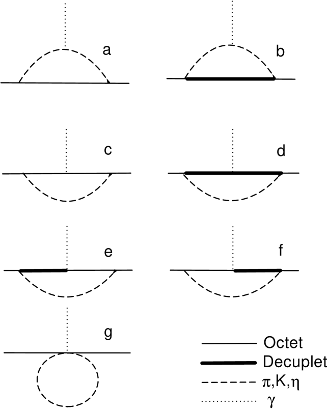
where $q=p^{\prime}-p$ and $Q^{2}=-q^{2}$. According to the Lagrangian, the one loop Feynman diagrams which contribute to the nucleon magnetic moments are plotted in Fig. 1. The contributions to nucleon magnetic form factors of Fig. 1a are expressed as

$$G_{M}^{p(1a)}=\frac{m_{N}(D+F)^{2}}{8\pi^{3}f_{\pi}^{2}}I_{1\pi}^{NN}+\frac{m_{N}(D+3F)^{2}I_{1K}^{N\Lambda}+3m_{N}(D-F)^{2}I_{1K}^{N\Sigma}}{{48\pi^{3}f_{\pi}^{2}}},$$ (25)

$$G_{M}^{n(1a)}=-\frac{m_{N}(D+F)^{2}}{8\pi^{3}f_{\pi}^{2}}I_{1\pi}^{NN}+\frac{m_{N}(D-F)^{2}}{8\pi^{3}f_{\pi}^{2}}I_{1K}^{N\Sigma}.$$ (26)

The integration $I_{1j}^{\alpha\beta}$ is expressed as

$$I_{1j}^{\alpha\beta}=\int d\overrightarrow{k}\frac{k_{y}^{2}u(\overrightarrow{k}+\overrightarrow{q}/2)u(\overrightarrow{k}-\overrightarrow{q}/2)(\omega_{j}(\overrightarrow{k}+\overrightarrow{q}/2)+\omega_{j}(\overrightarrow{k}-\overrightarrow{q}/2)+\delta^{\alpha\beta})}{A_{j}^{\alpha\beta}},$$ (27)

where

$$A_{j}^{\alpha\beta} = \omega_{j}(\overrightarrow{k}+\overrightarrow{q}/2)\omega_{j}(\overrightarrow{k}-\overrightarrow{q}/2)(\omega_{j}(\overrightarrow{k}+\overrightarrow{q}/2)+\delta^{\alpha\beta})$$ (28)

$$(\omega_{j}(\overrightarrow{k}-\overrightarrow{q}/2)+\delta^{\alpha\beta})(\omega_{j}(\overrightarrow{k}+\overrightarrow{q}/2)+\omega_{j}(\overrightarrow{k}-\overrightarrow{q}/2)).$$

$\omega_{j}(\overrightarrow{k})=\sqrt{m_{j}^{2}+\overrightarrow{k}^{2}}$ is the energy of the meson $j$. In our calculation we use the finite range regularisation and $u(\overrightarrow{k})$ is the ultra-violet regulator. This diagram is studied in the previous paper Young2 which gives the leading analytic term to the magnetic moments. The first terms in Eqs. (25) and (26) come from the $\pi$ meson cloud contribution. The second terms come from the K meson cloud contribution. Fig. 1b is the same as Fig. 1a but the intermediate states are decuplet baryons. Their contributions to the magnetic form factors are expressed as

$$G_{M}^{p(1b)}=\frac{m_{N}{\cal C}^{2}}{36\pi^{3}f_{\pi}^{2}}I_{1\pi}^{N\Delta}-\frac{m_{N}{\cal C}^{2}}{144\pi^{3}f_{\pi}^{2}}I_{1K}^{N\Sigma^{\ast}},$$ (29)

$$G_{M}^{n(1b)}=-\frac{m_{N}{\cal C}^{2}}{36\pi^{3}f_{\pi}^{2}}I_{1\pi}^{N\Delta}-\frac{m_{N}{\cal C}^{2}}{72\pi^{3}f_{\pi}^{2}}I_{1K}^{N\Sigma^{\ast}}.$$ (30)

The contributions to the form factors from Fig. 1c are expressed as

$$G_{M}^{p(1c)} = \frac{(D+F)^{2}(\mu_{D}-\mu_{F})}{192\pi^{3}f_{\pi}^{2}}I_{2\pi}^{NN}-\frac{1}{192\pi^{3}f_{\pi}^{2}}\left[(D-F)^{2}(2\mu_{F}+\mu_{D})I_{2K}^{N\Sigma}-(\frac{D}{3}+F)^{2}\mu_{D}I_{2K}^{N\Lambda}\right.$$ (31)

$$\left.-(D-F)(\frac{2D}{3}+2F)\mu_{D}I_{5K}^{N\Lambda\Sigma}\right]-\frac{(\frac{D}{3}-F)^{2}(\mu_{D}+3\mu_{F})}{192\pi^{3}f_{\pi}^{2}}I_{2\eta}^{NN},$$

$$G_{M}^{n(1c)} = -\frac{(D+F)^{2}\mu_{F}}{96\pi^{3}f_{\pi}^{2}}I_{2\pi}^{NN}-\frac{1}{192\pi^{3}f_{\pi}^{2}}\left[(D-F)^{2}(\mu_{D}-2\mu_{F})I_{2K}^{N\Sigma}-(\frac{D}{3}+F)^{2}\mu_{D}I_{2K}^{N\Lambda}\right.$$ (32)

$$\left.+(\frac{2D}{3}+2F)(D-F)\mu_{D}I_{5K}^{N\Lambda\Sigma}\right]+\frac{(\frac{D}{3}-F)^{2}\mu_{D}}{96\pi^{3}f_{\pi}^{2}}I_{2\eta}^{NN},$$

where

$$I_{2j}^{\alpha\beta}=\int d\overrightarrow{k}\frac{k^{2}u(\overrightarrow{k})^{2}}{\omega_{j}(\overrightarrow{k})(\omega_{j}(\overrightarrow{k})+\delta^{\alpha\beta})^{2}},$$ (33)

$$I_{5j}^{\alpha\beta\gamma}=\int d\overrightarrow{k}\frac{k^{2}u(\overrightarrow{k})^{2}}{\omega_{j}(\overrightarrow{k})(\omega_{j}(\overrightarrow{k})+\delta^{\alpha\beta})(\omega_{j}(\overrightarrow{k})+\delta^{\alpha\gamma}))}.$$ (34)

The magnetic moments of baryons in the chiral limit, expressed in terms of $\mu_{D}$ and $\mu_{F}$, are used in the one loop calculations. However, we have taken the mass difference of the octet baryons into account. If the masses of the octet baryons are taken to be degenerate, then the coefficients in front of the integrals will be the same as in the paper of Ref. Jenkins2 .

The contributions to the form factors of Fig. 1d are expressed as

$$G_{M}^{p(1d)}=\frac{5{\cal C}^{2}\mu_{C}}{162\pi^{3}f_{\pi}^{2}}I_{2\pi}^{N\Delta}+\frac{5{\cal C}^{2}\mu_{C}}{1296\pi^{3}f_{\pi}^{2}}I_{2K}^{N\Sigma^{\ast}},$$ (35)

$$G_{M}^{n(1d)}=-\frac{5{\cal C}^{2}\mu_{C}}{648\pi^{3}f_{\pi}^{2}}I_{2\pi}^{N\Delta}-\frac{5{\cal C}^{2}\mu_{C}}{1296\pi^{3}f_{\pi}^{2}}I_{2K}^{N\Sigma^{\ast}}.$$ (36)

Fig. 1e and Fig. 1f give the following contributions to the form factors:

$$G_{M}^{p(1e+1f)}=\frac{(D+F){\cal C}\mu_{T}}{108\pi^{3}f_{\pi}^{2}}I_{3\pi}^{N\Delta}+\frac{5(D-F){\cal C}\mu_{T}}{864\pi^{3}f_{\pi}^{2}}I_{5K}^{N\Sigma\Sigma^{\ast}}+\frac{(D+3F){\cal C}\mu_{T}}{864\pi^{3}f_{\pi}^{2}}I_{5K}^{N\Lambda\Sigma^{\ast}},$$ (37)

$$G_{M}^{n(1e+1f)}=-\frac{(D+F){\cal C}\mu_{T}}{108\pi^{3}f_{\pi}^{2}}I_{3\pi}^{N\Delta}+\frac{(D-F){\cal C}\mu_{T}}{864\pi^{3}f_{\pi}^{2}}I_{5K}^{N\Sigma\Sigma^{\ast}}-\frac{(D+3F){\cal C}\mu_{T}}{864\pi^{3}f_{\pi}^{2}}I_{5K}^{N\Lambda\Sigma^{\ast}},$$ (38)

where

$$I_{3j}^{\alpha\beta}=\int d\overrightarrow{k}\frac{k^{2}u(\overrightarrow{k})^{2}}{\omega_{j}(\overrightarrow{k})^{2}(\omega_{j}(\overrightarrow{k})+\delta^{\alpha\beta})}.$$ (39)

Fig. 1g comes from the second order expansion of Lagrangian (16). The contributions to the magnetic form factors are expressed as

$$G_{M}^{p(1g)}=-\frac{(\mu_{D}+\mu_{F})}{32\pi^{3}f_{\pi}^{2}}I_{4\pi}-\frac{\mu_{F}}{16\pi^{3}f_{\pi}^{2}}I_{4K},$$ (40)

$$G_{M}^{n(1g)}=\frac{(\mu_{D}+\mu_{F})}{32\pi^{3}f_{\pi}^{2}}I_{4\pi}+\frac{(\mu_{D}-\mu_{F})}{32\pi^{3}f_{\pi}^{2}}I_{4K},$$ (41)

where

$$I_{4j}=\int d\overrightarrow{k}\frac{u(\overrightarrow{k})^{2}}{\omega_{j}(\overrightarrow{k})}.$$ (42)

The magnetic moment is defined as $\mu=G_{M}(Q^{2}=0)$. The total nucleon magnetic moments can be written as

$$\mu_{p}(m_{\pi}^{2})=a^{p}_{0}+a^{p}_{2}m^{2}_{\pi}+a^{p}_{4}m^{4}_{\pi}+\sum_{k=a}^{g}G_{M}^{p(1k)}(Q^{2}=0,m_{\pi}^{2}),$$ (43)

$$\mu_{n}(m_{\pi}^{2})=a^{n}_{0}+a^{n}_{2}m^{2}_{\pi}+a^{n}_{4}m^{4}_{\pi}+\sum_{k=a}^{g}G_{M}^{n(1k)}(Q^{2}=0,m_{\pi}^{2}),$$ (44)

where $a^{N}_{0}$ ($N=n,p$) is expressed as

$$a^{N}_{0}=c^{N}_{0}-\sum_{k=a}^{g}G_{M}^{N(1k)}(Q^{2}=0,m_{\pi}^{2}=0).$$ (45)

$c^{p}_{0}$ ($c^{n}_{0}$) is $\mu_{p}$ ($\mu_{n}$) which is related to $\mu_{D}$ and $\mu_{F}$ via Eq. (18). The residual series parameters, $a_{i}$, are determined by the best fit of the lattice data.

Table 1: Residual series coefficients and nucleon form factors at zero momentum and 0.23 GeV². The first two rows provide standard results whereas the final row includes the effect of the pion form factor.

$Q^{2}$	$a_{0}^{p}$	$a_{0}^{n}$	$a_{2}^{p}$ (GeV-2)	$a_{2}^{n}$ (GeV-2)	$a_{4}^{p}$ (GeV-4)	$a_{4}^{n}$ (GeV-4)	$G_{M}^{p}$	$G_{M}^{n}$
0	2.554	$-$1.506	$-$1.135	0.420	0.446	$-$0.090	2.73 $\pm$ 0.20	$-$1.84 $\pm$ 0.19
0.23	1.617	$-$0.932	$-$0.411	0.070	0.144	0.031	1.70 $\pm$ 0.12	$-$1.10 $\pm$ 0.11
0.23	1.652	$-$0.968	$-$0.499	0.159	0.201	$-$0.027	1.65 $\pm$ 0.10	$-$1.06 $\pm$ 0.09

IV Numerical results

In the numerical calculations, the parameters are chosen as $D=0.76$ and $F=0.50$ ($g_{A}=D+F=1.26$). The coupling constant ${\cal C}$ is chosen to be $-1.2$ which is the same as Ref. Jenkins2 . The renormalisation form factor $u(k)$ can be monopole, dipole or Gaussian functions which give similar results Young2 . In our calculations, the dipole function is used:

$$u(k)=\frac{1}{(1+k^{2}/\Lambda^{2})^{2}},$$ (46)

with $\Lambda=0.8$ GeV. The coefficients $a^{p}_{0}$, $a^{n}_{0}$, $a^{p}_{2}$, $a^{n}_{2}$, $a^{p}_{4}$ and $a^{n}_{4}$ in Eqs. (43) and (44) are constrained by the quenched lattice data at large pion mass ($m_{\pi}>500$ MeV) where the quenched and physical values of the magnetic moments are expected to be close to each other Leinweber0 ; Young:2004tb .

The $K$- and $\eta$-meson masses have relationships with the pion mass according to

$$m_{K}^{2}=\frac{1}{2}m_{\pi}^{2}+m_{K}^{2}|_{\rm phy}-\frac{1}{2}m_{\pi}^{2}|_{\rm phy},$$ (47)

$$m_{\eta}^{2}=\frac{1}{3}m_{\pi}^{2}+m_{\eta}^{2}|_{\rm phy}-\frac{1}{3}m_{\pi}^{2}|_{\rm phy}\,,$$ (48)

and enable a direct relationship between the meson dressings of the nucleon magnetic moments and the pion mass.

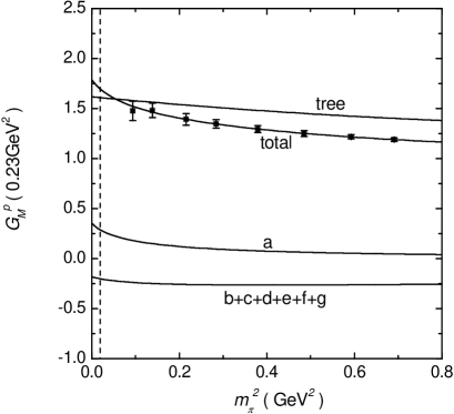
We begin by considering nucleon form factor results from the CSSM Lattice Collaboration Boinepalli:2006xd . The proton magnetic moment $\mu_{p}$ versus $m_{\pi}^{2}$ is shown in Fig. 2. Here, the last five lattice points at larger $m_{\pi}^{2}$ are used in the fit to avoid quenched chiral artifacts. The lines with label a and b+c+d+e+f+g correspond to the contributions of Fig. 1a and sum of the other diagrams, respectively. The residual series contribution, i.e. the contribution from $a_{0}+a_{2}m_{\pi}^{2}+a_{4}m_{\pi}^{4}$ is also shown in the figure and labeled by “tree”. The near linear behavior of the residual series is a reflection of the excellent convergence of the residual expansion.

Figure 2: The proton magnetic moment Boinepalli:2006xd versus squared pion mass. The lines with label a and b+c+d+e+f+g correspond to the contributions of Fig. 1a and the sum of the other diagrams, respectively.

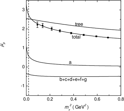
The leading diagram (Fig. 1a) gives the dominant chiral behavior of the magnetic moment. At small pion mass, the proton magnetic moment decreases quickly with the increasing pion mass. At larger pion mass, the proton magnetic moment changes smoothly. At the physical point, $m_{\pi}=0.139$ GeV, the proton magnetic moment is $2.73\ \mu_{N}$, close to the experimental value, $2.79\ \mu_{N}$. We emphasize again that the chiral curvature is dominated by Fig. 1a.

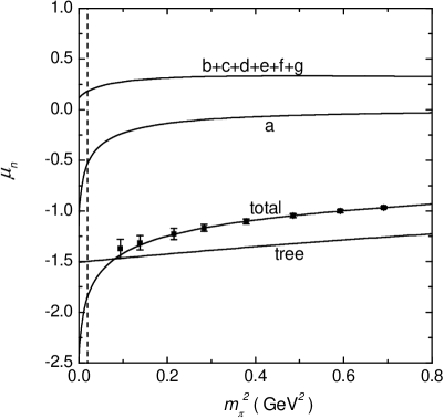
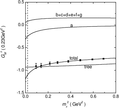
The neutron magnetic moment, $\mu_{n}$, is studied in the same way. $\mu_{n}$ versus $m_{\pi}^{2}$ is shown in Fig. 3. Again, only the five lattice points at larger pion mass are used in the fit to avoid quenched chiral artifacts. Similar to what was found in proton case, the leading diagram gives the dominant chiral curvature. The neutron magnetic moment increases quickly as ones moves from the chiral limit and becomes smooth at large pion mass. At the physical point, the neutron magnetic moment is $-1.84\ \mu_{N}$, compares favorably with the experimental value of $-1.91\mu_{N}$. For both the proton and neutron, the rapid variation of the magnetic moments at $m_{\pi}=0$ may reflect the fact that the nucleon magnetic radii diverge in the chiral limit.

Figure 3: The neutron magnetic moment Boinepalli:2006xd versus squared pion mass. The lines with label a and b+c+d+e+f+g correspond to the contributions of Fig. 1a and the sum of the other diagrams, respectively.

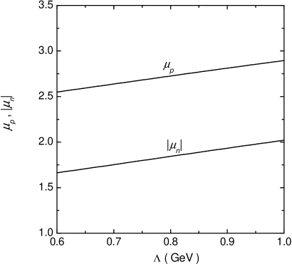
In the above numerical calculations, we selected $\Lambda$ to be 0.8 GeV. In Fig. 4 we show the nucleon magnetic moments versus $\Lambda$. The proton magnetic moment and the absolute value of neutron magnetic moment increase almost linearly with increasing $\Lambda$. In the range $0.6<\Lambda<1.0$ GeV, the proton (neutron) magnetic moment varies from $2.55\ \mu_{N}$ ($-1.66\ \mu_{N}$) to $2.90\ \mu_{N}$ ($-2.02\ \mu_{N}$). When $\Lambda$ is around 0.8 GeV, both the proton and neutron magnetic moments are in good agreement with the experimental values.

Since the extrapolated values are $\Lambda$ dependent (an indication that the fits lie outside the power-counting regime), the uncertainty of $\Lambda$ will result in an additional source of error in the final result. Through a consideration of optimizing the convergence properties of the finite-range regularised expansion, we include the variation of $\Lambda$ in the range 0.8 $\pm$ 0.2 GeV and add this uncertainty to the statistical uncertainties in quadrature. The extrapolated magnetic moments with corresponding error bars are listed in table I.

In the chiral limit, the magnetic moments, $c_{0}^{p}$ and $c_{0}^{n}$, are 3.41 and -2.53. These two values are close to the corresponding ones used in normal chiral perturbation theory. For example, in Ref. Fuchs:2003ir , the corresponding values are 3.38 and -2.66. For the higher order terms, our low energy constants are much smaller, resulting in more convergent behavior. For example, our $a_{2}^{p}$ and $a_{2}^{n}$ are $-1.14$ and 0.42 which are much smaller than the corresponding values $-6.80$ and 8.75 in Ref. Fuchs:2003ir .

Figure 4: The proton and neutron magnetic moments versus the regulator scale $\Lambda$.

We now proceed to extrapolate the nucleon magnetic form factors at finite $Q^{2}$. At finite momentum transfer, we choose not to express the magnetic form factors in terms of $Q^{2}$ and $Q^{4}$ as we did for the $m_{\pi}$ dependence of $\mu_{N}$. This is because the momentum dependence of form factors is close to the following assumption $G_{M}^{N}(Q^{2})=\mu_{N}/(1+Q^{2}/0.71$GeV${}^{2})^{2}$. The high order terms in a $Q^{2}$ expansion are important and the truncation of momentum to some order, say fourth order, is not a good approximation.

In our calculation, the same formulas as Eqs. (43) and (44) are used for the extrapolation of the magnetic form factors at each fixed finite value of $Q^{2}$. The $Q^{2}$ dependence of nucleon magnetic form factors at tree level is included in the parameters $a_{0}$, $a_{2}$ and $a_{4}$, as these parameters are constrained by the lattice results at finite $Q^{2}$.

In addition to the CSSM Lattice collaboration results Boinepalli:2006xd considered thus far, we also consider QCDSF lattice results at finite $Q^{2}$ QCDSF . Large statistical uncertainties encountered at large $Q^{2}$ prevent one from constraining the $m_{\pi}^{4}$ term and therefore we fit the QCDSF data using a residual series expansion up to and including order $m_{\pi}^{2}$ only. The coefficients together with the form factors at finite $Q^{2}$ are obtained by fitting the lattice results and are listed in Tables I and II. From the tables, one can see that $a_{0}^{p}$ decreases with increasing momentum, while $a_{0}^{n}$ increases with momentum. $a_{2}^{N}$ (N=p,n) are small indicating good convergence of the expansion.

Table 2: Residual series coefficients and nucleon form factors at various $Q^{2}$. The first four lines report standard results while the latter four lines report results including the effect of a pion form factor.

$Q^{2}$ (GeV2)	$a_{0}^{p}$	$a_{0}^{n}$	$a_{2}^{p}$ (GeV-2)	$a_{2}^{n}$ (GeV-2)	$G_{M}^{p}$	$G_{M}^{n}$
0.557	1.042	$-$0.638	$-$0.024	$-$0.00	1.07 $\pm$ 0.17	$-$0.71 $\pm$ 0.14
1.08	0.609	$-$0.337	0.015	$-$0.04	0.61 $\pm$ 0.13	$-$0.37 $\pm$ 0.13
1.14	0.598	$-$0.348	0.052	$-$0.04	0.59 $\pm$ 0.11	$-$0.37 $\pm$ 0.09
2.28	0.293	$-$0.178	0.035	$-$0.03	0.28 $\pm$ 0.09	$-$0.18 $\pm$ 0.05
0.557	1.051	$-$0.650	$-$0.033	0.01	1.01 $\pm$ 0.15	$-$0.66 $\pm$ 0.10
1.08	0.620	$-$0.349	0.008	$-$0.03	0.58 $\pm$ 0.12	$-$0.34 $\pm$ 0.12
1.14	0.610	$-$0.360	0.044	$-$0.04	0.57 $\pm$ 0.10	$-$0.35 $\pm$ 0.07
2.28	0.300	$-$0.185	0.032	$-$0.02	0.27 $\pm$ 0.09	$-$0.17 $\pm$ 0.05

We plot the $m_{\pi}$ dependence of proton and neutron magnetic form factors at $Q^{2}=0.23$ GeV² in Figs. 5 and 6 respectively. At small pion mass, the proton and neutron magnetic form factors do not change as quickly as in the case of zero momentum. However, the diagram of Fig. 1a still gives the dominant contribution to the curvature when the pion mass is small. From the figures, one can see that the expansion in powers of $m_{\pi}$ shows good convergence. At the physical pion mass, $G_{M}^{p}(0.23$ GeV${}^{2})=(1.70$ $\pm$ 0.12) $\mu_{N}$ and $G_{M}^{n}(0.23$ GeV${}^{2})=-1.10$ $\pm$ 0.11) $\mu_{N}$, which are both reasonable compared with experiment.

Figure 5: The proton magnetic form factor Boinepalli:2006xd at $Q^{2}=0.23$ GeV² versus the squared pion mass. The lines with label a and b+c+d+e+f+g correspond to the contributions of Fig. 1a and the sum of the other diagrams respectively.

Figure 6: The neutron magnetic form factor Boinepalli:2006xd at $Q^{2}=0.23$ GeV² versus squared pion mass. The lines with label a and b+c+d+e+f+g correspond to the contributions of Fig. 1a and the sum of the other diagrams respectively.

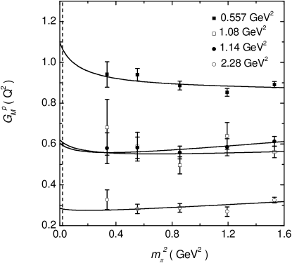
In Figs. 7 and 8, we plot the proton and neutron magnetic form factors respectively. Results at $Q^{2}=0.557$, 1.08, 1.14 and 2.28 GeV² from the QCDSF collaboration QCDSF are considered. From the figures, one can see that the lattice data do not vary smoothly as a function of the pion mass due to large statistical errors. As a consequence, the extrapolated magnetic form factors at the physical pion mass have relatively large error bars. Accurate lattice results are needed to better constrain the chiral expansion parameters and allow one to consider an $m_{\pi}^{4}$ term in the residual expansion.

Figure 7: The proton magnetic form factors QCDSF at $Q^{2}=0.557$, 1.08, 1.14 and 2.28 GeV² versus pion mass.

Figure 8: The neutron magnetic form factors QCDSF at $Q^{2}=0.557$, 1.08, 1.14 and 2.28 GeV² versus pion mass.

To this point, we have not considered the possibility of an important role for the pion form factor in the calculation. We know that at large $Q^{2}$, the pion form factor is much less than one and this will affect the meson cloud contribution to nucleon magnetic form factors. We list the pion electromagnetic form factor $F_{\pi}$ in Table III as provided in Ref. Melo .

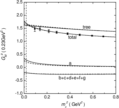
With these pion form factors, we repeat the chiral fit of the nucleon magnetic form factors. As an example, in Fig. 9, we show the result obtained for the proton magnetic form factor at $Q^{2}$=0.23 GeV². The dashed and solid lines are for the results with and without the pion form factor consideration, respectively. When the pion form factor is included, the leading diagram Fig. 1a provides less curvature. As a result, the total $G_{M}^{P}$ decreases from 1.70 $\pm$ 0.12 $\mu_{N}$ to 1.65 $\pm$ 0.10 $\mu_{N}$. For the neutron, $G_{M}^{n}$ increases from $-1.10$ $\pm$ 0.11 $\mu_{N}$ to $-1.06$ $\pm$ 0.09 $\mu_{N}$. Though the pion form factor changes significantly at finite momentum, it does not affect the nucleon magnetic form factors very much. At large $Q^{2}$, the pion form factor has a negligible effect on the nucleon form factors because the loop contribution itself is already very small.

Table 3: Pion electromagnetic form factor, $F_{\pi}$, at various $Q^{2}$.

$Q^{2}$ (GeV2)	0.23	0.557	1.08	1.14	2.28
$F_{\pi}$	0.70	0.50	0.31	0.29	0.18

Figure 9: The proton magnetic form factor Boinepalli:2006xd at $Q^{2}=0.23$ GeV² versus pion mass. The dashed and solid lines are for the results with and without the pion form factor, respectively.

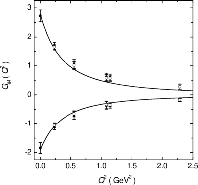
In Fig. 10, we show the extrapolated proton and neutron magnetic form factors versus $Q^{2}$ at the physical pion mass with the corresponding error bars. The hollow and solid square points are for the fits with and without the pion form factor, respectively.

The solid lines in Fig. 10 are the empirical parametrization $G_{M}^{N}(Q^{2})=\mu_{N}/(1+Q^{2}/0.71$GeV${}^{2})^{2}$. At both zero momentum and $Q^{2}=0.23$ GeV², the extrapolated CSSM results are in good agreement with the experimental data. For the other values of $Q^{2}$ from the QCDSF collaboration, the extrapolated nucleon magnetic form factors are in reasonable agreement with the empirical parameterization. For the neutron the agreement is quite reasonable, while for the proton, although the extrapolation is consistently within one standard deviation of the empirical curve, the extrapolated values do appear to be systematically a little high.

We should mention that we use just two parameters, $a_{0}$ and $a_{2}$, to fit the lattice data (at each value of $Q^{2}$). We note that it would be very helpful to have more accurate lattice data over a range of lattice spacings and volumes in order to extrapolate to the infinite volume continuum limit and to be able to incorporate an $a_{4}$ term. One would also prefer to work with full QCD data rather than quenched data. Until these conditions are satisfied it is a little early to draw strong conclusions about the validity of the extrapolation in pion mass from a comparison with experimental data for the form factors. Indeed, that the current results lie within one standard deviation of the data at all values of $Q^{2}$ is really a very positive result at the present stage. We do emphasis that our results are based on the lowest order Lagrangian at one loop level in heavy baryon approximation. That must breakdown at high momentum transfer, however, that is precisely where, in the FRR treatment, the loops become naturally small – for the clear physical reason that high pion momenta (and high pion mass) are suppressed by the finite size of the source. The extrapolation error arising from the uncertainty in $\Lambda$ included above is small when the momentum is high. Again, this is because at high momentum transfer, the loop contribution to the total magnetic form factor is small.

Figure 10: The proton and neutron magnetic form factors at physical pion mass versus the momentum transfer, $Q^{2}$. The hollow and solid square points are for the fits with and without the inclusion of the form factor of the pion, respectively.

V summary

We extrapolated state of the art lattice results for nucleon magnetic form factors in an extension of heavy baryon chiral perturbation theory. All one-loop graphs are considered at arbitrary momentum transfer and all octet and decuplet baryons are included in the intermediate states.

Finite-range regularisation is used in the one loop calculation to improve the convergence of the chiral expansion. The residual series coefficients $a_{0}^{p}$($a_{0}^{n}$), $a_{2}^{p}$ ($a_{2}^{n}$) and $a_{4}^{p}$ ($a_{4}^{n}$) are obtained by fitting the lattice results at $m_{\pi}>0.5$ GeV, where quenched artifacts are anticipated to be small.

The leading non-analytic diagram provides the dominant curvature for the $m_{\pi}$ dependence of magnetic moments. The sum of higher-order one-loop terms provide only a small correction to this curvature. The one-loop contributions show that the proton (neutron) magnetic moment decreases (increases) quickly with increasing pion mass in the small $m_{\pi}$ region. At larger pion masses, their contributions change slowly and smoothly.

The magnetic form factors are also studied at large $Q^{2}$ where chiral nonanalytic behavior is suppressed. Here, the importance of the pion form factor is also examined. For $Q^{2}=0.23$ GeV², $G_{M}^{p}=1.70\pm 0.12\ \mu_{N}$ and $G_{M}^{n}=-1.10\pm 0.11\ \mu_{N}$. Upon including the pion form factor, these values will change to $1.65\pm 0.10\ \mu_{N}$ and $-1.06\pm 0.09\ \mu_{N}$ indicating the effect is subtle. Although the pion form factor decreases quickly with increasing momentum, its effect on nucleon form factors is not significant, as the loop integrals themselves are already small.

The chirally extrapolated results of Fig. 10 compare favorably with experiment and demonstrate the utility and accuracy of the chiral extrapolation methods presented herein. With the more accurate lattice data and treatment, it is of interest to see whether the mismatch at large $Q^{2}$ will disappear or not.

References

- (1) H. Y. Gao, Int. J. Mod. Phys. E 12, 1 (2003) [Erratum-ibid. E 12, 567 (2003)] [arXiv:nucl-ex/0301002].
- (2) C. E. Hyde-Wright and K. de Jager, Ann. Rev. Nucl. Part. Sci. 54, 217 (2004) [arXiv:nucl-ex/0507001].
- (3) J. Arrington, C. D. Roberts and J. M. Zanotti, arXiv:nucl-th/0611050.
- (4) C. F. Perdrisat, V. Punjabi and M. Vanderhaeghen, arXiv:hep-ph/0612014.
- (5) D. B. Leinweber, W. Melnitchouk, D. G. Richards, A. G. Williams and J. M. Zanotti, Lect. Notes Phys. 663, 71 (2005) [arXiv:nucl-th/0406032].
- (6) D. B. Leinweber, R. M. Woloshyn and T. Draper, Phys. Rev. D 43, 1659 (1991).
- (7) D. B. Leinweber et al., Phys. Rev. Lett. 94, 212001 (2005) [arXiv:hep-lat/0406002].
- (8) D. B. Leinweber et al., Phys. Rev. Lett. 97, 022001 (2006) [arXiv:hep-lat/0601025].
- (9) R. G. Edwards et al. [LHPC Collaboration], Phys. Rev. Lett. 96, 052001 (2006) [arXiv:hep-lat/0510062].
- (10) S. Boinepalli, D. B. Leinweber, A. G. Williams, J. M. Zanotti and J. B. Zhang, Phys. Rev. D 74, 093005 (2006).
- (11) M. Gockeler et al. [QCDSF Collaboration], Phys. Rev. D 71, 034508 (2005) [arXiv:hep-lat/0303019].
- (12) D.B. Leinweber and T.D. Cohen, Phys. Rev D 47, 2147 (1993).
- (13) D.B. Leinweber, A.W. Thomas and R.D. Young, Phys. Rev. Lett. 86, 5011 (2001).
- (14) T.R. Hemmert and W. Weise, Eur. Phys. J. A 15, 487 (2002).
- (15) D. B. Leinweber, A. W. Thomas, K. Tsushima and S. V. Wright, Phys. Rev. D 61, 074502 (2000) [arXiv:hep-lat/9906027].
- (16) W. Detmold et al., Phys. Rev. Lett. 87, 172001 (2001) [arXiv:hep-lat/0103006].
- (17) S. Weinberg, Physica 96A (1979) 327.
- (18) J. Gasser, M. E. Sainio and A. Svarc, Nucl. Phys. B 307, 779 (1988).
- (19) E. Jenkins and A. V. Manohar, Phys. Lett. B 255, 558 (1991).
- (20) P. Ha and L. Durand, Phys. Rev. D bf 58, 093008 (1998); Phys. Rev. D 67, 073017 (2003).
- (21) B. Kubis and U. G. Meissner, Nucl. Phys. A 679, 698 (2001).
- (22) B. Borasoy and U. G. Meissner, Annals Phys. 254, 192 (1997) [arXiv:hep-ph/9607432].
- (23) D. B. Leinweber, A. W. Thomas and R. D. Young, Phys. Rev. Lett. 92, 242002 (2004).
- (24) M. Procura, T. R. Hemmert and W. Weise, Phys. Rev. D 69, 034505 (2004).
- (25) T. R. Hemmert, M. Procura and W. Weise, Phys. Rev. D 68, 075009 (2003).
- (26) D.B. Leinweber, A. W. Thomas, K. Tsushima and S. V. Wright, Phys. Rev. D 61, 074502 (2000).
- (27) W. Armour, C. R. Allton, D. B. Leinweber, A. W. Thomas and R. D. Young, J. Phys. G 32, 971 (2006) [arXiv:hep-lat/0510078].
- (28) C. R. Allton, W. Armour, D. B. Leinweber, A. W. Thomas and R. D. Young, Phys. Lett. B 628 (2005) 125 [arXiv:hep-lat/0504022].
- (29) J. F. Donoghue, B. R. Holstein and B. Borasoy, Phys. Rev. D 59, 036002 (1999).
- (30) R. D. Young, D. B. Leinweber and A. W. Thomas, Prog. Nucl. Phys. 50, 399 (2003).
- (31) R. D. Young, D. B. Leinweber and A. W. Thomas, Phys. Rev. D 71, 014001 (2005) [arXiv:hep-lat/0406001].
- (32) V. Bernard, N. Kaiser, J. Kambor and U. G. Meissner, Nucl. Phys. B 388, 315 (1992).
- (33) V. Bernard, H. W. Fearing, T. R. Hemmert and U. G. Meissner, Nucl. Phys. A 635, 121 (1998) [Erratum-ibid. A 642, 563 (1998)] [arXiv:hep-ph/9801297].
- (34) T. Fuchs, J. Gegelia and S. Scherer, J. Phys. G 30, 1407 (2004) [arXiv:nucl-th/0305070].
- (35) V. Bernard, N. Kaiser and U. G. Meissner, Nucl. Phys. A 611, 429 (1996)
- (36) N. Kaiser, Phys. Rev. C 68, 025202 (2003) [arXiv:nucl-th/0302072].
- (37) M. R. Schindler, J. Gegelia and S. Scherer, Eur. Phys. J. A 26, 1 (2005) [arXiv:nucl-th/0509005].
- (38) C. Alexandrou, G. Koutsou, J. W. Negele and A. Tsapalis, Phys. Rev. D 74, 034508 (2006) [arXiv:hep-lat/0605017].
- (39) M. Gockeler et al., arXiv:hep-lat/0609001.
- (40) R. G. Edwards et al., arXiv:hep-lat/0610007.
- (41) E. Jenkins, M. Luke, A. V. Manohar and M. J. Savage, Phys. Lett. B 302, 482 (1993); Erratum-ibid. B 388, 866 (1996).
- (42) J. N. Labrenz and S. Sharpe, Phys. Rev. D 54, 4595 (1996).
- (43) L. Durand, P. Ha, and G. Jaczko, Phys. Rev. D 64, 014008 (2001).
- (44) B. C. Tiburzi, Phys. Rev. D 71, 054504 (2005) [arXiv:hep-lat/0412025].
- (45) J. P. B. C. de Melo, J. S. Veiga, T. Frederico, E. Pace and G. Salme, hep-ph/0609212.