One-loop Radiative Corrections to the $\rho$ Parameter in the Left Right Twin Higgs Model

Abstract

We implement a one-loop analysis of the $\rho$ parameter in the Left Right Twin Higgs model, including the logarithmically enhanced contributions from both heavy fermion and scalar loops. Numerical analysis indicates that the one-loop corrections are dominant over the tree-level contributions in most regions of parameter space. The experimentally allowed values of the $\rho$-parameter divide the allowed parameter space into two regions; less than $670~{}{\rm GeV}$ and larger than $1100~{}{\rm GeV}$ roughly, for the symmetry breaking scale $f$. Therefore our result significantly reduces the parameter space which are favorably accessible to the LHC.

I Introduction

The Standard Model (SM) has excellently described high energy physics up to energies of ${\mathcal{O}}(100)$ GeV. The only undetected constituent of the SM to date is a Higgs boson which is essential to generating fermion and gauge boson masses. Theoretically the Higgs boson mass squared is quadratically sensitive to any new physics scale beyond the Standard Model (BSM) and stabilization of the Higgs mass squared prefers the energy scale below ${\mathcal{O}}(1)$ TeV. But electroweak precision measurements with naive naturalness assumption raise the energy scale of the BSM up to 100 TeV or even higher. Hence, there remains a tension between theory and experiment associated with the stabilization of the SM Higgs mass. With the latest data from the LHC the tension gets stronger.

The basic idea of little Higgs is that the SM Higgs is a pseudo-Nambu-Goldstone boson(pNGB) Georgi:1974yw ; Kaplan:1983fs ; Arkani-Hamed:2001nc ; Arkani-Hamed:2002pa ; Arkani-Hamed:2002qx ; Arkani-Hamed:2002qy ; Schmaltz:2002wx . Stabilization of the Higgs mass in the little Higgs theories is achieved by the “collective symmetry breaking” which naturally renders the SM Higgs mass much smaller than the global symmetry breaking scale. The distinct elements of little Higgs models are a vector-like heavy top quark, and various scalar and vector bosons. The former is universal while the latter is model-dependent. Both of them contribute significantly to one-loop processes and hence set strict constraints on the parameter space of little Higgs models. At worst, electroweak precision tests push up the symmetry breaking scale to $5$ TeV or higher, and even revive the fine-tuning problem of the Higgs potential.

The basic idea of twin Higgs is the same as that of little Higgs. But the stabilization of the Higgs mass squared is different between the two. The twin Higgs mechanism introduces additional discrete symmetry to render no quadratic divergence in the Higgs mass squared. For instance, the mirror twin Higgs model containing a complete copy of the SM identifies the discrete symmetry with mirror parity. The SM world and its mirror world communicate only through the Higgs so that the mirror particles are very elusive in the SM world and yield poor phenomenology at the LHC.

The twin Higgs mechanism can be also realized by identifying the discrete symmetry with left-right symmetry in the left-right model Chacko:2005un . The left-right twin Higgs (LRTH) model contains $U(4)_{1}\times U(4)_{2}$ global symmetry as well as $SU(2)_{L}\times SU(2)_{R}\times U(1)_{B-L}$ gauge symmetry. The left-right symmetry acts on only the two $SU(2)$’s gauge symmetry. A pair of vector-like heavy top quarks play a key role in triggering electroweak symmetry breaking just as that of the little Higgs theories. On top of that, the non-SM Higgs particles acquire large masses not only at quantum level but also at tree level, making the model deliver much richer phenomenology at the LHC Goh:2006wj compared with the mirror twin Higgs model. Moreover they lead to large radiative corrections to one-loop processes so the allowed parameter space can be significantly reduced. In this paper we perform a one-loop analysis of the $\rho$-parameter in the LRTH model to reduce the parameter space.

The paper is organized as follows. The LRTH model is briefly reviewed in Section 2. The renormalization procedure for $\rho$-parameter is explained in Section 3. The numerical analysis on the $\rho$-parameter is performed in Section 4. We present our conclusions in Section 5. The technical details on the computation of the $\rho$-parameter are reckoned in Appendices.

II Left right twin Higgs model in a nutshell

We review the LRTH model in Ref. Goh:2006wj . The LRTH model is based on the global $U(4)_{1}\times U(4)_{2}$ symmetry, with a locally gauged subgroup $SU(2)_{L}\times SU(2)_{R}\times U(1)_{B-L}$. A pair of Higgs fields, $H$ and $\hat{H}$, are introduced and each transforms as $(4,1)$ and $(1,4)$, respectively, under the global symmetry. They are written as

$$H=\left(\begin{array}[]{c}H_{L}\\ H_{R}\end{array}\right),\qquad\hat{H}=\left(\begin{array}[]{c}\hat{H}_{L}\\ \hat{H}_{R}\end{array}\right),$$ (1)

where $H_{L,R}$ and $\hat{H}_{L,R}$ are two component objects which are charged under the $SU(2)_{L}\times SU(2)_{R}\times U(1)_{B-L}$ as

$$H_{L}\mbox{ and }\hat{H}_{L}\,:\,(2,1,1),\qquad H_{R}\mbox{ and }\hat{H}_{R}\,:\,(1,2,1).$$ (2)

The global $U(4)_{1}\,(U(4)_{2})$ symmetry is spontaneously broken down to its subgroup $U(3)_{1}\,(U(3)_{2})$ with VEVs

$$\langle H\rangle^{T}=(0,0,0,f),\qquad\langle\hat{H}\rangle^{T}=(0,0,0,\hat{f}).$$ (3)

The spontaneous symmetry breaking results in seven Nambu-Goldstone bosons (NGB), which are parameterized as

$$H=fe^{\pi/f}\left(\begin{array}[]{c}0\\ 0\\ 0\\ 1\end{array}\right),\qquad\qquad\pi=\left(\begin{array}[]{cccc}-\frac{N}{2\sqrt{3}}&0&0&h_{1}\\ 0&-\frac{N}{2\sqrt{3}}&0&h_{2}\\ 0&0&-\frac{N}{2\sqrt{3}}&C\\ h^{\ast}_{1}&h^{\ast}_{2}&C^{\ast}&\frac{\sqrt{3}N}{2}\end{array}\right),$$ (4)

where $\pi$ is the corresponding Goldstone field matrix. $N$ is a neutral real field , $C$ and $C^{\ast}$ are a pair of charged complex scalar fields, and $h_{SM}=(h_{1},h_{2})$ is the SM $SU(2)_{L}$ Higgs doublet. $\hat{H}$ is parameterized in the identical way by its own Goldstone boson matrix, $\hat{\pi}$, which contains $\hat{N}$, $\hat{C}$, and $\hat{h}=(\hat{h}^{+}_{1},\hat{h}^{0}_{2})$. The two $U(4)/U(3)$’s symmetry breakings yield fourteen NGBs in all.

The linear combination of $C$ and $\hat{C}$, and the linear combination of $N$ and $\hat{N}$ are eaten by the gauge bosons of $SU(2)_{R}\times U(1)_{B-L}$, which is broken down to the $U(1)_{Y}$. The orthogonal linear combinations, a charged complex scalar $\phi^{\pm}$ and a neutral real pseudoscalar $\phi^{0}$, remain as NGBs. On top of that, the SM Higgs acquires a VEV, $\langle h_{SM}\rangle=(0,v/\sqrt{2})$, so electroweak symmetry $SU(2)_{L}\times U(1)_{Y}$ is broken down to $U(1)_{EM}$. But $\hat{h}$’s do not get a VEV and remain as NGBs. At the end of the day, the two Higgs VEVs are given by

$$\langle H\rangle=\left(\begin{array}[]{c}0\\ if\sin x\\ 0\\ f\cos x\end{array}\right),\qquad\langle\hat{H}\rangle=\left(\begin{array}[]{c}0\\ 0\\ 0\\ \hat{f}\end{array}\right),\$$ (5)

where $x=\frac{v}{\sqrt{2}f}$. The values of $f$ and $\hat{f}$ will be bounded by electroweak precision measurements. In addition, $f$ and $\hat{f}$ are interconnected once we set $v=246$ GeV.

II.1 Gauge sector

The whole gauge symmetry of the model is $SU(3)_{C}\times SU(2)_{L}\times SU(2)_{R}\times U(1)_{B-L}$. But since $SU(3)_{C}$ is irrelevant to eletroweak symmetry breaking $SU(3)_{C}$ gauge symmetry is not taken into account in this paper. The generators of the $SU(2)_{L}\times SU(2)_{R}\times U(1)_{B-L}$ is given respectively as,

$$\left(\begin{array}[]{cc}\frac{1}{2}\sigma_{i}&0\\ 0&0\end{array}\right),\qquad\left(\begin{array}[]{cc}0&0\\ 0&\frac{1}{2}\sigma_{i}\end{array}\right),\qquad\frac{1}{2}\left(\begin{array}[]{cc}1_{2}&0\\ 0&1_{2}\end{array}\right),$$ (6)

and the corresponding gauge fields are $W^{\pm,0}_{L},W^{\pm,0}$ and $B$, respectively. The covariant derivative is then given as

$$D_{\mu}=\partial_{\mu}-ig{\mathcal{W}}_{\mu}-ig^{\prime}q_{B-L}{\mathcal{B}}_{\mu},$$ (7)

where

$${\mathcal{W}}=\frac{1}{2}\left(\begin{array}[]{cccc}W^{0}_{L}&\sqrt{2}W^{+}_{L}&0&0\\ \sqrt{2}W^{-}_{L}&-W^{0}_{L}&0&0\\ 0&0&W^{0}_{R}&\sqrt{2}W^{+}_{R}\\ 0&0&\sqrt{2}W^{-}_{R}&-W^{0}_{R}\end{array}\right),\qquad{\mathcal{B}}=\frac{1}{2}\left(\begin{array}[]{cccc}B&0&0&0\\ 0&B&0&0\\ 0&0&B&0\\ 0&0&0&B\end{array}\right),$$ (8)

and $g$ and $g^{\prime}$ are the gauge couplings for $SU(2)_{L,R}$ and $U(1)_{B-L}$, and $q_{B-L}$ is the charge of the field under $U(1)_{B-L}$.

The kinetic term for the two Higgs fields can be written as

$${\mathcal{L}}_{H}=(D_{\mu}H)^{\dagger}D^{\mu}H+(D_{\mu}\hat{H})^{\dagger}D^{\mu}\hat{H}$$ (9)

with $q_{B-L}=1$. The Higgs mechanism for both $H$ and $\hat{H}$ makes the six gauge bosons massive but one gauge boson, photon, massless. For the charged gauge bosons, there is no mixing between the $W^{\pm}_{L}$ and $W^{\pm}_{R}$: $W^{\pm}_{L}$ is identified with the SM weak gauge boson $W^{\pm}$ while $W^{\pm}_{R}$ is much heavier than $W^{\pm}$ and is denoted as $W^{\pm}_{H}$. Their masses are

$$M^{2}_{W}=\frac{1}{2}g^{2}f^{2}\sin^{2}x,\qquad M^{2}_{W_{H}}=\frac{1}{2}g^{2}(\hat{f}^{2}+f^{2}\cos^{2}x).$$ (10)

Note that $M^{2}_{W}+M^{2}_{W_{H}}=\frac{g^{2}}{2}(f^{2}+\hat{f}^{2})$. The linear combinations of the neutral gauge bosons $W^{0}_{L},W^{0}_{R}$ and $B$ yield two neutral massive gauge bosons $Z,Z_{H}$ and one photon $A$ with masses, respectively:

$$M^{2}_{A} =0,$$ (11)

$$M^{2}_{Z} =\frac{g^{2}+2g^{\prime 2}}{g^{2}+g^{\prime 2}}\frac{2M^{2}_{W}M^{2}_{W_{H}}}{M^{2}_{W_{H}}+M^{2}_{W}+\sqrt{(M^{2}_{W_{H}}-M^{2}_{W})^{2}+\frac{4g^{\prime 2}}{g^{2}+g^{\prime 2}}M^{2}_{W_{H}}M^{2}_{W}}},$$ (12)

$$M^{2}_{Z_{H}} =\frac{g^{2}+g^{\prime 2}}{g^{2}}(M^{2}_{W}+M^{2}_{W_{H}})-M^{2}_{Z}.$$ (13)

For later use, we define the Weinberg angle of the LRTH model:

$$s_{w} =\sin\theta_{w}=\frac{g^{\prime}}{\sqrt{g^{2}+2g^{\prime 2}}},$$ (14)

$$c_{w} =\cos\theta_{w}=\sqrt{\frac{g^{2}+g^{\prime 2}}{g^{2}+2g^{\prime 2}}},$$ (15)

$$c2_{w} =\sqrt{\cos 2\theta_{w}}=\frac{g}{\sqrt{g^{2}+2g^{\prime 2}}}.$$ (16)

The unit of the electric charge is then given by

$$e=gs_{w}=\frac{gg^{\prime}}{\sqrt{g^{2}+2g^{\prime 2}}}.$$ (17)

II.2 Fermion sector

To cancel the quadratic sensitivity of the Higgs mass to the top quark loops, a pair of vector-like, charge $2/3$ fermion $({\mathcal{Q}}_{L},{\mathcal{Q}}_{R})$ are incorporated into the top Yukawa sector,

$${\mathcal{L}}_{Yuk}=y_{L}\bar{Q}_{L3}\tau_{2}H^{\ast}_{L}{\mathcal{Q}}_{R}+y_{R}\bar{Q}_{R3}\tau_{2}H^{\ast}_{R}{\mathcal{Q}}_{L}-M\bar{\mathcal{Q}}_{L}{\mathcal{Q}_{R}}+h.c.,$$ (18)

where $\tau_{2}=\left(\begin{array}[]{cc}0&-1\\ 1&0\end{array}\right)$, $Q_{L3}=-i(u_{L3},d_{L3})$ and $Q_{R3}=(u_{R3},d_{R3})$ are the third generation up- and down-type quarks, respectively. The left-right parity indicates $y_{L}=y_{R}(\equiv y)$. The mass parameter $M$ is essential to the top mixing. The value of $M$ is constrained by the $Z\to b\bar{b}$ branching ratio. It can be also constrained by the oblique parameters, which we will do in the letter. Furthermore, it yields large log divergence of the SM Higgs mass. To compensate for it the non-SM gauge bosons also get large masses by increasing the value of $\hat{f}$. Therefore it is natural for us to take $M\lesssim yf$.

Expanding the $H_{L,R}$ field in terms of NGB fields, we acquire the mass matrix of the fermions. By diagonalizing it we obtain not only the mass eigenstates for the SM-like and heavy top quarks, but also the mixing angles for the left-handed and right-handed fermions:

$$m^{2}_{t} =\frac{1}{2}(M^{2}+y^{2}f^{2}-N_{t}),\quad m^{2}_{T}=\frac{1}{2}(M^{2}+y^{2}f^{2}+N_{t}),$$ (19)

$$\sin\alpha_{L} =\frac{1}{\sqrt{2}}\sqrt{1-(y^{2}f^{2}\cos 2x+M^{2})/N_{t}},$$ (20)

$$\sin\alpha_{R} =\frac{1}{\sqrt{2}}\sqrt{1-(y^{2}f^{2}\cos 2x-M^{2})/N_{t}},$$ (21)

where $N_{t}=\sqrt{(y^{2}f^{2}+M^{2})^{2}-y^{4}f^{4}\sin^{2}2x}$.

II.3 Higgs sector

Among the fourteen NGBs in both $\pi$ and $\hat{\pi}$, six NGBs are eaten by the gauge bosons. The remaining eight NGBs get masses through quantum effects and/or soft symmetry breaking terms, so called “$\mu$-term”. The Coleman-Weinberg potential, obtained by integrating out the heavy gauge bosons and top quarks, yields the SM Higgs potential, which determines the SM Higgs VEV and its mass, as well as the masses for the other Higgs, $\phi^{\pm},\phi^{0},\hat{h}^{\pm}_{1}$ and $\hat{h}^{0}_{2}$. Moreover, the $\mu$-term contributes to the Higgs masses at tree level :

$$V_{\mu}=-\mu^{2}_{r}(H^{\dagger}_{R}\hat{H}_{R}+c.c.)+\hat{\mu}^{2}\hat{H}^{\dagger}_{L}\hat{H}_{L}.$$ (22)

We write down the masses for the Higgs.

$$M^{2}_{\phi^{0}} =\frac{\mu^{2}_{r}f\hat{f}}{\hat{f}^{2}+f^{2}\cos^{2}x}\Big{[}\frac{\hat{f}^{2}(\cos x+\frac{\sin x}{x}(4+x^{2}))}{f^{2}(\cos x+2\frac{\sin x}{x})^{2}}+\frac{2\cos x(\cos x+4\frac{\sin x}{x})}{3(\cos x+2\frac{\sin x}{x})}$$

$$\qquad\qquad\qquad+\frac{f^{2}\cos^{2}x(4+\cos x)}{9\hat{f}^{2}}\Big{]},$$ (23)

$$M^{2}_{\phi^{\pm}} =\frac{3}{16\pi^{2}}\frac{g^{\prime 2}M^{2}_{W_{H}}}{M^{2}_{Z_{H}}-M^{2}_{Z}}\Big{[}\Big{(}\frac{M^{2}_{W}}{M^{2}_{Z_{H}}}-1\Big{)}{\mathcal{Z}}(M_{Z_{H}})-\Big{(}\frac{M^{2}_{W}}{M^{2}_{Z}}-1\Big{)}{\mathcal{Z}}(M_{Z})\Big{]}$$

$$\,+\frac{\mu^{2}_{r}f\hat{f}}{\hat{f}^{2}+f^{2}\cos^{2}x}\Big{[}\frac{\hat{f}^{2}x^{2}}{f^{2}\sin^{2}x}+2\cos x+\frac{f^{2}\cos^{3}x}{\hat{f}^{2}}\Big{]},$$ (24)

$$M^{2}_{\hat{h}_{2}} =\frac{3}{16\pi^{2}}\Big{[}\frac{g^{2}}{2}({\mathcal{Z}}(M_{W})-{\mathcal{Z}}(M_{W_{H}}))+\frac{2g^{\prime 2}+g^{2}}{4}\frac{M^{2}_{W_{H}}-M^{2}_{W}}{M^{2}_{Z_{H}}-M^{2}_{Z}}({\mathcal{Z}}(M_{Z})-{\mathcal{Z}}(M_{Z_{H}}))\Big{]}$$

$$\,+\mu^{2}_{r}\frac{f}{\hat{f}}\cos x+\hat{\mu}^{2},$$ (25)

$$M^{2}_{\hat{h}_{1}} =M^{2}_{\hat{h}_{2}}+\frac{3}{16\pi^{2}}\frac{g^{\prime 2}M^{2}_{W}}{M^{2}_{Z_{H}}-M^{2}_{Z}}\Big{[}\Big{(}\frac{M^{2}_{W_{H}}}{M^{2}_{Z_{H}}}-1\Big{)}{\mathcal{Z}}(M_{Z_{H}})-\Big{(}\frac{M^{2}_{W_{H}}}{M^{2}_{Z}}-1\Big{)}{\mathcal{Z}}(M_{Z})\Big{]}.$$ (26)

where

$${\mathcal{Z}}(x)=-x^{2}(\ln\frac{\Lambda^{2}}{x^{2}}+1),$$ (27)

with $\Lambda$ being a UV cutoff. The SM Higgs potential arises mainly from both top and gauge sector. The contribution of fermion loop to the SM Higgs mass squared is negative and its dominance over the contribution of gauge boson loops and tree level mass parameter $\mu_{r}^{2}\frac{\hat{f}}{2f}$ triggers electroweak symmetry breaking. We fix the SM Higgs VEV, $v=246~{}{\rm GeV}$.

III The renormalization procedure

We follow the renormalization procedure in Ref. Chen:2003fm to calculate the $\rho$-parameter at one-loop order. The $Z$-pole, $W$-mass, and neutral current data can be used to search for and set limits on deviations from the SM. The the $\rho$-parameter is defined as

$$\rho\equiv\frac{M^{2}_{W}}{M^{2}_{Z}c^{2}_{\theta}}.$$ (28)

The electroweak mixing angle $s^{2}_{\theta}(\equiv 1-c^{2}_{\theta})$ in the effective leptonic (electronic) vertex of the Z boson is defined as

$$s^{2}_{\theta}\equiv\frac{1}{4}\Big{(}1+\mbox{Re}\,\frac{g^{e}_{V}}{g^{e}_{A}}\Big{)},$$ (29)

in terms of the effective vector and axial vector couplings $g^{e}_{V,A}$ of the $Z$ to electrons;

$${\cal L}=i\bar{e}\gamma_{\mu}(g_{V}+g_{A}\gamma_{5})eZ^{\mu}.$$ (30)

The effective Lagrangian of the charged current interaction in the LRTH model is given by

$${\mathcal{L}}_{cc}=\frac{g}{\sqrt{2}}\big{(}W_{\mu L}^{+}J^{\mu-}_{L}+W^{-}_{\mu L}J^{\mu+}_{L}\big{)}+(L\to R),$$ (31)

where $J^{\mu\pm}_{L,R}$ is the charged currents. For momenta quite small compared to $M_{W}$, this effective Lagrangian gives rise to the effective four-fermion interaction with the Fermi coupling constant,

$$\frac{G_{F}}{\sqrt{2}}=\frac{g^{2}}{8M^{2}_{W}},$$ (32)

and the vector and axial vector parts of the neutral current $Zee$ coupling constants are given to the order $v^{2}/\hat{f}^{2}$ as,

$$g^{e}_{V} =\frac{g}{2c_{w}}\Big{[}\big{(}-\frac{1}{2}+2s^{2}_{w}\big{)}+\frac{v^{2}}{4(f^{2}+\hat{f}^{2})}\frac{s^{2}_{w}(c2^{2}_{w}-2)}{c^{4}_{w}}\Big{]},$$ (33)

$$g^{e}_{A} =\frac{g}{2c_{w}}\Big{[}\frac{1}{2}+\frac{v^{2}}{4(f^{2}+\hat{f}^{2})}\frac{s^{2}_{w}c2^{2}_{w}}{c^{4}_{w}}\Big{]}.$$ (34)

The effective leptonic mixing angle $s^{2}_{\theta}$ in Eq. (29) is then related to the mixing angle $s^{2}_{w}$ as

$$s^{2}_{\theta}=s^{2}_{w}-\frac{v^{2}}{f^{2}+\hat{f}^{2}}\frac{s^{4}_{w}}{c^{2}_{w}}.$$ (35)

It can then be inverted and gives

$$s^{2}_{w}=s^{2}_{\theta}+\Delta s^{2}_{\theta},$$ (36)

where

$$\frac{\Delta s^{2}_{\theta}}{s^{2}_{\theta}}=-\zeta+\frac{1}{2}\frac{c^{2}_{\theta}}{s^{2}_{\theta}}-\sqrt{-\zeta+\Big{(}\zeta-\frac{1}{2}\frac{c^{2}_{\theta}}{s^{2}_{\theta}}\Big{)}^{2}},$$ (37)

with

$$\zeta\equiv\frac{v^{2}}{f^{2}+\hat{f}^{2}}.$$ (38)

The SM $SU(2)_{L}$ gauge coupling constant, $g$, is expressed by both the effective leptonic mixing angle, $s^{2}_{\theta}$, and the fine-structure constant, $\alpha$, as

$$g^{2}=\frac{e^{2}}{s^{2}_{w}}=\frac{4\pi\alpha}{s^{2}_{\theta}}\big{(}1-\frac{\Delta s^{2}_{\theta}}{s^{2}_{\theta}}\big{)}.$$ (39)

The $\rho$-parameter at tree level is

$$\rho^{tree}=\frac{\pi\alpha}{\sqrt{2}G_{F}c^{2}_{\theta}s^{2}_{\theta}M^{2}_{Z}}\big{(}1-\frac{\Delta s^{2}_{\theta}}{s^{2}_{\theta}}\big{)}.$$ (40)

The $\rho$-parameter at the tree level is differentiated from unity and its deviation from unity is of order $v^{2}/\hat{f}^{2}$.

Since the loop factor arising from radiative corrections, $1/16\pi^{2}$, is similar in magnitude to $v^{2}/\hat{f}^{2}$ (for $\hat{f}\gtrsim 5$ TeV), the one-loop radiative corrections can be comparable in size to the next-to-leading order corrections at tree level. At one-loop order the mass relation reads Sirlin:1980nh

$$s^{2}_{\theta}c^{2}_{\theta}=\frac{\pi\alpha(M_{Z})}{\sqrt{2}G_{F}M^{2}_{Z}\rho}\Big{[}1-\frac{\Delta s^{2}_{\theta}}{s^{2}_{\theta}}+\Delta r_{Z}\Big{]},$$ (41)

where $\Delta r_{Z}$ includes radiative effects from various sources:

$$\Delta r_{Z}=\frac{\delta\alpha}{\alpha}-\frac{\delta G_{F}}{G_{F}}-\frac{\delta M^{2}_{Z}}{M^{2}_{Z}}-\Big{(}\frac{c^{2}_{\theta}-s^{2}_{\theta}}{c^{2}_{\theta}}\Big{)}\frac{\delta s^{2}_{\theta}}{s^{2}_{\theta}}.$$ (42)

We should mention that $\Delta r_{Z}$ in Eq. (42) differs from the usual $\Delta\hat{r}_{Z}$ defined in the SM by an extra corrections due to the renormalization of $s^{2}_{\theta}$. In general, The vertex and box contributions to the radiative effects are relatively small compared to the other corrections Sirlin:1980nh ; Blank:1997qa and hence we consider only the so-called “oblique” type, i.e. the $W$-, $Z$- and $\gamma$-propagators. The correction due to the vacuum polarization of the photon, $\delta\alpha$, is given by

$$\frac{\delta\alpha}{\alpha}=\Pi^{\gamma\gamma^{\prime}}(0)+2\Big{(}\frac{g^{e}_{V}-g^{e}_{A}}{Q_{e}}\Big{)}\frac{\Pi^{\gamma Z}(0)}{M^{2}_{Z}}.$$ (43)

Since we ignore the vertex and box corrections, the electroweak radiative correction to the Fermi constant, $\delta G_{F}$, stems from the $W$-boson vacuum polarization,

$$\frac{\delta G_{F}}{G_{F}}=-\frac{\Pi^{WW}(0)}{M^{2}_{W}}.$$ (44)

The counterterms for the $Z$-boson mass, $\delta M^{2}_{Z}$, and the leptonic mixing angle, $\delta s^{2}_{\theta}$, are given by, respectively Blank:1997qa

$$\delta M^{2}_{Z} =Re[\Pi^{ZZ}(M^{2}_{Z})],$$ (45)

$$\frac{\delta s^{2}_{\theta}}{s^{2}_{\theta}} =Re\Big{[}\Big{(}\frac{c_{\theta}}{s_{\theta}}\Big{)}\Big{\{}\frac{\Pi^{\gamma Z}(M^{2}_{Z})}{M^{2}_{Z}}+\frac{v^{2}_{e}-a^{2}_{e}}{a_{e}}\Sigma^{e}_{A}(m^{2}_{e})-\frac{v_{e}}{2s_{\theta}c_{\theta}}\Big{(}\frac{\Lambda^{Z\bar{e}e}_{V}(M^{2}_{Z})}{v_{e}}-\frac{\Lambda^{Z\bar{e}e}_{A}(M^{2}_{Z})}{a_{e}}\Big{)}\Big{\}}\Big{]},$$ (46)

where $\Lambda^{Z\bar{e}e}_{V,A}$ are the vector and axial vector form factors of the unnormalized one-loop $Zee$ vertex corrections, and $\Sigma^{e}_{A}$ is the axial part of the electron self-energy. Once again, we ignore these “non-oblique” type corrections.

The tree level and radiative corrections except for the W-boson are summed up and expressed as

$$\Delta\hat{r}=-\frac{\Delta s^{2}_{\theta}}{s^{2}_{\theta}}-\frac{Re[\Pi^{ZZ}(M^{2}_{Z})]}{M^{2}_{Z}}+\Pi^{\gamma\gamma^{\prime}}(0)+2\Big{(}\frac{g^{e}_{V}-g^{e}_{A}}{Q_{e}}\Big{)}\frac{\Pi^{\gamma Z}(0)}{M^{2}_{Z}}-\frac{c^{2}_{\theta}-s^{2}_{\theta}}{c_{\theta}s_{\theta}}\frac{Re[\Pi^{\gamma Z}(M^{2}_{Z})]}{M^{2}_{Z}},$$ (47)

and then Eq. (41) is rewritten as,

$$s^{2}_{\theta}c^{2}_{\theta}=\frac{\pi\alpha(M_{Z})}{\sqrt{2}G_{F}M^{2}_{Z}\rho}\Big{[}1+\frac{\Pi^{WW}(0)}{M^{2}_{W}}+\Delta\hat{r}\Big{]}.$$ (48)

Solving Eq. (28) and (48) for the $W$-boson mass we get it as

$$M^{2}_{W}=\frac{1}{2}\Big{[}a(1+\Delta\hat{r})+\sqrt{a^{2}(1+\Delta\hat{r})^{2}+4a\Pi^{WW}(0)}\Big{]},$$ (49)

with $\quad a\equiv\frac{\pi\alpha(M_{Z})}{\sqrt{2}G_{F}s^{2}_{\theta}}$. Finally the $\rho$ parameter is calculated using Eq. (28).

IV Numerical Analysis

In order to take the precision measurements, we need the standard experimental values as input parameters. These are the input parameters we take Yao:2006px :

$$G_{F} =1.16637(1)\times 10^{-5}\mbox{ GeV}^{-2},$$ (50)

$$M_{Z} =91.1876(21)\mbox{ GeV},$$ (51)

$$\alpha(M_{Z})^{-1} =127.918(18),$$ (52)

$$s^{2}_{\theta} =0.23153(16).$$ (53)

We also take the top and bottom quark masses as  Yao:2006px ; Rodrigo:1997gy

$$m_{t}=172.3~{}{\rm GeV},\qquad m_{b}=3~{}{\rm GeV},$$ (54)

where $m_{t}$ is the central value of the electroweak fit and $m_{b}$ is the running mass at the $M_{Z}$ scale with $\overline{MS}$ scheme. The $\rho$-parameter itself is measured very accurately Yao:2006px ,

$$\rho \equiv\rho_{0}\hat{\rho}\equiv\frac{M^{2}_{W}}{M^{2}_{Z}c^{2}_{\theta}}$$ (55)

$$\rho_{0} =1.0002^{+0.0007}_{-0.0004}$$ (56)

$$\hat{\rho} =1.01043\pm 0.00034$$ (57)

Including all the SM corrections (top quark loop, bosonic loops), we take the allowed range of $\rho$ parameter as

$$1.00989~{}\leq~{}\rho^{exp}~{}\leq~{}1.01026.$$ (58)

Figure 1: Plots of $\hat{f}$ versus $f$ with different values of $M$.

The input parameters of the LRTH model are as follows;

$$f,~{}M,~{}\mu_{r},~{}\hat{\mu},$$ (59)

where $M$ is the heavy top quark mass scale, both $\mu_{r}$ and $\hat{\mu}$ are soft symmetry breaking terms. The masses of the top and heavy top quarks are determined mainly by $f$ and $M$ while those of the scalar particles $\hat{h}_{1},~{}\hat{h}_{2},~{}\phi^{\pm}$ and $\phi^{0}$ largely depend on $\hat{\mu},~{}\mu_{r}$ and $f$. Another scale $\hat{f}$, associated with the masses of the heavy gauge bosons, can be determined by the electroweak symmetry breaking condition: there is a generic relation between $\hat{f}$ and $f$ since Coleman-Weinberg potential of the Higgs boson mostly depends on $M,f$ and $\hat{f}$. For scalar potential, there is a tree level mass term proportional to $\mu_{r}^{2}$. So we may not acquire negative mass squared term which is necessary for electroweak symmetry breaking and it gives an upper bound for the value of $\mu_{r}$.

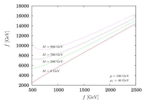
Figure 1 shows $f$ versus $\hat{f}$ with various values of the heavy top mass scale, $M$. For a given $f$, $\hat{f}$ becomes larger as $M$ increases. The heavy top loop through $M$ contributes positively to the Higgs mass while the heavy gauge boson loop through $\hat{f}$ contributes negatively to the Higgs mass. The two contributions cancel out in order to retain $v=246$ GeV. There is also a contribution from tree level mass term $~{}\mu_{r}^{2}$, but in most cases it make little difference to the relation as long as $\mu_{r}$ is much smaller than the Higgs mass scale. This insensitiveness can be figured out with simple evaluation. First, from the electroweak symmetry breaking condition, the mass squared contribution from the soft symmetry breaking term $\mu_{r}^{2}\frac{\hat{f}}{2f}$ should be smaller than that from the fermion loop. This can be written down approximately as follows:

$$\mu_{r}^{2}\frac{\hat{f}}{2f}<\frac{3}{8\pi^{2}}(M^{2}+y^{2}f^{2}).$$ (60)

In the above inequality, we ignore the gauge boson loop contributions since they are small compared to the fermion loop contributions. In general $\hat{f}$ is larger than $f$ about $5$ times or more and $\frac{3}{8\pi^{2}}$ is very small, we can see that $\mu_{r}$ should be very much smaller than $f$. To get the $\hat{f}$ which reproduces the electroweak symmetry breaking scale $v=246$ GeV, we should solve the equation,

$$\frac{3g^{4}}{64\pi^{2}}f{\hat{f}}^{2}+\mu_{r}^{2}\hat{f}+2\lambda v^{2}f-\frac{3}{4\pi^{2}}f(M^{2}+f^{2})+\frac{3g^{4}}{64\pi^{2}}=0,$$ (61)

for given $f,M$ and $\mu_{r}$. $\lambda$ in the above equation is the coefficient of quartic term and less than $1$ in general. Note that we derive the above equation with some degree of approximation. For example, we ignore the logarithmic terms. But the crude behavior will be similar. In this equation, the coefficients of $\hat{f}^{2}$ and $\hat{f}$ are much smaller than constant term, so the solution $\hat{f}$ is almost insensitive to the value of $\mu_{r}$ .

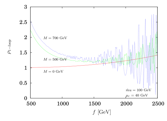
Plots in Figure 2 illustrate the behavior of one-loop $\rho$-parameter for various values of $M$. At $M=0$, where there is no mixing between the top and heavy top quarks, $\Delta\rho$ increases monotonically with $f$. For nonzero $M$ where the mixing is turned on, mass of the heavy top quark becomes large as $M$ increases for a given $f$, and the fermionic loop contributions tend to become large, too. The effects of mixing angles on the fermionic loops become significant as either $f$ or $M$ increases while the condition of electroweak symmetry breaking is retained. In other words, since the mixing angles are determined by $f$ and $M$, the one-loop corrected $\rho$ parameter begins to waver as $f$ increases even with the fixed scalar mass parameters. Because of this nature, fine tuning in the $\rho$-parameter is inevitable for large $f$, as will be shown later.

Figure 2: The plot for the $\rho$-parameter versus $f$ with different values of $M$.

To extract a meaningful information on the model parameters from the $\rho$-parameter, we scan the parameter space generally, i.e.,

$$500~{}{\rm GeV}~{}\leq~{}f~{}\leq~{}2500~{}{\rm GeV},~{}~{}~{}~{}~{}~{}0~{}\leq~{}M,~{}\mu_{r},~{}\hat{\mu}~{}\leq~{}f.$$ (62)

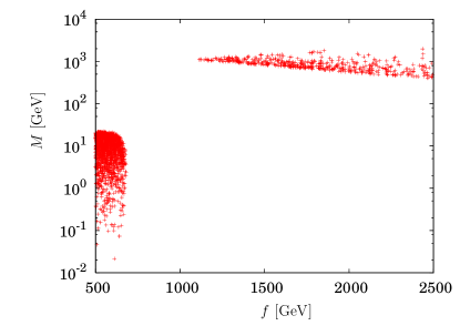
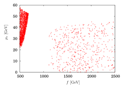
Even though too large $f$ makes the model unviable, we take the rather large value of $f$, 2.5 TeV, as an upper limit for completeness of the scanning. As a result of $\rho$-parameter calculation, we can obtain the allowed regions of parameter space. As an example, Figure 3 shows the allowed regions of parameter space (a) for $f$ versus $M$ and (b) for $f$ versus $\mu_{r}$. It is interesting to notice that the allowed parameter space is divided into two regions; less than 670 GeV and larger than 1100 GeV roughly, for $f$. This can be figured out as follows. The loop corrections tend to be larger as $f$ increases. It is because the masses of the particles involved in one-loop correction increase in general as $f$ increases. But at the same time, the mixing angles of top-heavy top quarks also vary. Since the mixing angles depend on not only $f$ but also $M$, these two effects compete during the increase of $f$. Because of this interplay of top mixing angles and masses, we have two distinct allowed parameter spaces. For small $f$, solution points prefer very small values of $M$. It means there is no large mixing between the top and heavy top quarks. In general, $\Pi^{WW}(0)$ is large for small $f$, and decreases as $f$ increases. So for fitting the observed W-boson mass in the small $f$ region, which is directly related to the $\rho$-parameter, we restrict the $\Delta\hat{r}$ within rather small range. Because the $\Delta\hat{r}$ is mostly determined by $\Pi^{ZZ}(M_{Z}^{2})$, it should be also small. For doing that, we should take the small value of $M$, which makes the masses and mixing angles of heavy top quark small. We find that in the small $f$ region, $M$ should be smaller than about $22~{}{\rm GeV}$. Soft symmetry breaking parameter $\mu_{r}$ is restricted to the values less than around $60~{}{\rm GeV}$. This bound arises mainly from the electroweak symmetry breaking condition, and is generically independent of the $\rho$-parameter. Another free parameters $\hat{\mu}$ is not restricted from the one-loop corrected $\rho$-parameter. The reason is that $\hat{\mu}$ only contributes to the masses of $\hat{h}_{1}$ and $\hat{h}_{2}$, and their contributions are effectively cancelled among the relevant loop diagrams. It is pointed out in Appendix C.

Figure 3: (a) The scatter plot for the mass parameter $M$ with the horizontal axis being the scale parameter $f$. (b) The scatter plot for the mass parameter $\mu_{r}$ with the horizontal axis being the scale parameter $f$.

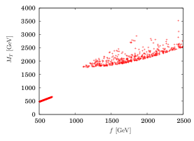
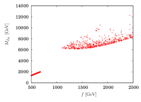
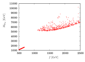
This region of parameter space can provide constraints on the masses of many particles appear in this model. First, let us consider the masses of the heavy top and heavy gauge bosons. As shown in Figure 4, their masses generically increase as $f$ increases. The mass of the heavy top quark is uniquely determined when $f,\hat{f}$ and $M$ are fixed. So does the top Yukawa coupling. Basically $\hat{f}$ is determined by the electroweak symmetry breaking condition, but their $M$ and $\mu_{r}$ dependence provoke the ambiguity on its value. For small $f$ region, since $M$ is also very small, the $M_{T}$ is almost determined by $f$ alone. It appears as straight line in Figure 4 (a). For large $f$ region, it becomes spread due to the top mixing angles. The plots of the heavy $Z$ and $W$ boson masses versus $f$ are quite similar to that of the heavy top mass versus $f$. In the case of heavy $W$ boson, the strongest constraint come from $K_{L}-K_{S}$ mixing. The strongest bound ever known is $m_{W_{H}}>1.6$ TeV, with the assumption of $g_{L}=g_{R}$. Beall:1981ze This can exclude some region from Figure 4(c). In this case, small $f$ region can be completely excluded, but the analysis of Ref. Beall:1981ze did not include the higher order QCD corrections and used vacuum insertion to obtain the matrix element. So we will not consider that bound seriously here. Detailed study including QCD corrections and others is being done by authors of Ref. Goh:2006wj . If the lower bound for $f$ is confirmed, we can give the lower bound for $f$ as $1.1~{}{\rm TeV}$ from our calculation of the $\rho$-parameter and also for many particles appear in the model. Another constraints on the $m_{W_{H}}$ from CDF and D0 are about $650\sim 786{\rm GeV}$, as lower bound Affolder:2001gr ; Abachi:1995yi . For Our results remain safe from these experimental bounds. Heavy $Z$ boson has also been studied in detail by many experimentalists. Current experimental bound is about $500\sim 800{\rm GeV}$ from precision measurements Yao:2006px and $\sim 630{\rm GeV}$ from CDF Yao:2006px . In this case, also safe is the mass of heavy $Z$ boson.

Figure 4: (a) The scatter plot for the heavy top mass with the horizontal axis being the scale parameter $f$. (b) The scatter plot for the heavy $Z$ boson mass with the horizontal axis being the scale parameter $f$. (c) The scatter plot for the heavy $W$-boson mass with the horizontal axis being the scale parameter $f$.

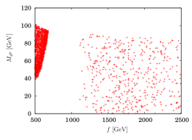
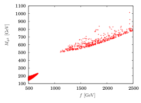
With the parameters allowed by the $\rho$-parameter, the masses of new scalar bosons $\hat{h}_{1,2},\phi^{0}$ and $\phi^{\pm}$ can be constrained. $\hat{h}_{1,2}$ have almost degenerate masses, and are dependent on both $\mu_{r}$ and $\hat{\mu}$, unlike the $\phi^{0,\pm}$ which depend only on $\mu_{r}$. Their masses are substantially constrained according to the value of $f$. Unfortunately, we cannot give a lower bound on the mass of $\phi^{0}$. In fact, its mass, though it is quite small, arise from radiative corrections. For $\phi^{\pm}$, the loop effects are rather large so they are heavier than $\phi^{0}$ as shown in Figure 5.

Figure 5: (a) The scatter plot for the mass of $\hat{h}_{1}$ with the horizontal axis being the scale parameter $f$. It is similar to that of $\hat{h}_{2}$. (b) The scatter plot for the mass of $\phi^{0}$ with the horizontal axis being the scale parameter $f$. (c) The scatter plot for the mass of $\phi^{+}1$ with the horizontal axis being the scale parameter $f$.

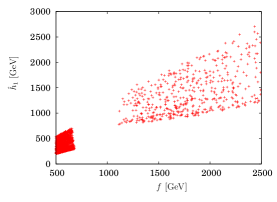
The distribution of the SM Higgs mass as a function of $f$ is shown in Figure 6. As for the lower bound of the SM Higgs mass we adopt the LEP bound for Higgs mass, $114.4~{}{\rm GeV}$ Barate:2003sz , since its structure is same as the SM. Its upper bound is approximately given as $167{\rm GeV}$.

Figure 6: The scatter plot for the SM Higgs mass with the horizontal axis being the scale parameter $f$.

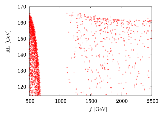
We summarize the results of our analysis as follows. With the observed $\rho$-parameter, the allowed parameter space is divided into two separate regions: $f$ smaller than about 670 GeV and larger than about 1.1 TeV. We can give the mass bounds of the particles in the LRTH model for either region. But the heavy gauge bosons remain safe from the experimental constraints. Unlike the other particles, we cannot set a lower bound for the neutral $\phi^{0}$ scalar. The loop corrections play an important role on the charged $\phi^{\pm}$ scalars, yielding mass difference between the charged and neutral scalars. Further analysis is required to reduce the allowed region. If the small $f$ region is excluded, for example by Ref. Goh:2006wj , we can provide exact lower bounds for the masses of $T,Z_{H},W_{H},\hat{h}_{1,2}$, and $\phi^{\pm}$. But even in that case, we cannot do so for $\phi^{0}$ and SM Higgs boson.

V Conclusion

The left right twin Higgs model is a concrete realization of the twin Higgs mechanism. The model predicts a heavy top quark, heavy gauge and various scalar bosons along with a light SM Higgs boson, and will in turn yield rich phenomenology of the new particles at the LHC. We have performed an indirect search for the existence of the particles. The heavy Top and new scalars contribute significantly to the isospin violating the $\rho$-parameter. One-loop radiative corrections to the $\rho$-parameter reduce parameter space of the model and can set rough bounds for the masses of the heavy particles. In particular, we demonstrated that the symmetry breaking parameter $f$ can be either smaller than $660~{}{\rm GeV}$ or larger than $1.1~{}{\rm TeV}$, which is a crucial region in parameter space. More analysis on other one-loop processes as well as study of collider physics is mandatory to further reduce the region of parameter space.

Appendix A Coupling constants of the LRTH model

We summarize the relevant coupling constants relevant to our calculation. The gauge-fermion interaction is given by

$${\mathcal{L}} =i\bar{\psi}_{1}\gamma_{\mu}(g_{V}+g_{A}\gamma_{5})\psi_{2}X^{\mu}$$

$$=i\bar{\psi}_{1}\gamma_{\mu}(c_{L}P_{L}+c_{R}P_{R})\psi_{2}X^{\mu},$$ (63)

where $P_{L,R}=\frac{1}{2}(1\mp\gamma_{5})$ are the projection operators. We make a list of the gauge coupling constants of the fermions in Table 1.

Table 1: Relevant coupling constants $X\bar{\psi}\psi$. The mixing angles $C_{L}=\cos\alpha_{L},C_{R}=\cos\alpha_{R}$, etc are given in Eq. (19).

$X\bar{\psi}\psi$
$W\bar{t}b$	$c_{L}=eC_{L}/(\sqrt{2}s_{w})$	$c_{R}=0$
$W\bar{T}b$	$c_{L}=eS_{L}/(\sqrt{2}s_{w})$	$c_{R}=0$
$Z\bar{t}t$	$g_{V}=e(\frac{1}{4}C^{2}_{L}-\frac{2}{3}s_{w}^{2})/(c_{w}s_{w})$	$g_{A}=-\frac{1}{4}eC_{L}^{2}/(c_{w}s_{w})$
$Z\bar{b}b$	$g_{V}=e(-\frac{1}{2}+\frac{2}{3}s^{2}_{w})/(2c_{w}s_{w})$	$g_{A}=e/(4c_{w}s_{w})$
$Z\bar{T}T$	$g_{V}=e(\frac{1}{4}S^{2}_{L}-\frac{2}{3}s_{w}^{2})/(c_{w}s_{w})$	$g_{A}=-\frac{1}{4}eS_{L}^{2}/(c_{w}s_{w})$
$Z\bar{T}t$	$c_{L}=eC_{L}S_{L}/(2c_{w}s_{w})$	$c_{R}=ef^{2}x^{2}s_{w}C_{R}S_{R}/(2\hat{f}^{2}c^{3}_{w})$
$A\bar{f}f$	$g_{V}=eQ_{f}$	$g_{A}=0$

The other gauge-scalar interactions are also taken into account. We choose the unitary gauge where all gauge-scalar mixing terms vanish. The various gauge coupling constants of the scalar fields are given in Table 2, 3, and 4.

Table 2: Relevant gauge coupling of the scalar fields, $C_{XSS}$. $p1$, $p2$ and $p3$ refer to the incoming momentum of the first, second and third particle, respectively Han:2003wu .

$XSS$	$C_{XSS}$	$XSS$	$C_{XSS}$
$W^{+}\hat{h}^{\dagger}_{1}\hat{h}_{2}$	$-e(p_{2}-p_{3})_{\mu}/(\sqrt{2}s_{w})$	$A\hat{h}^{\dagger}_{1}\hat{h}_{1}$	$-e(p_{2}-p_{3})_{\mu}$
$Z\hat{h}^{\dagger}_{1}\hat{h}_{1}$	$-e(c^{2}_{w}-s^{2}_{w})(p_{2}-p_{3})_{\mu}/(2c_{w}s_{w})$	$Z\hat{h}^{\dagger}_{2}\hat{h}_{2}$	$e(p_{2}-p_{3})_{\mu}/(2c_{w}s_{w})$
$Z\phi^{-}\phi^{+}$	$e(p_{2}-p_{3})_{\mu}s_{w}/c_{w}$	$A\phi^{-}\phi^{+}$	$-e(p_{2}-p_{3})_{\mu}$
$Zh\phi^{0}$	$iexp_{1\mu}/(6c_{w}s_{w})$

Table 3: Relevant gauge coupling constants of the scalar fields, $C_{XXSS}$ Han:2003wu .

$XXSS$	$C_{XXSS}$	$XXSS$	$C_{XXSS}$
$W^{+}W^{-}hh$	$e^{2}/(2s^{2}_{w})$	$ZZhh$	$e^{2}/(2c^{2}_{w}s^{2}_{2})$
$W^{+}W^{-}\phi^{0}\phi^{0}$	$-e^{2}x^{2}/(54s^{2}_{w})$	$ZZ\phi^{0}\phi^{0}$	$-e^{2}x^{2}/(54c^{2}_{w}s^{2}_{w})$
$W^{+}W^{-}\phi^{+}\phi^{-}$	$-e^{2}x^{2}/(6s^{2}_{w})$	$ZZ\phi^{+}\phi^{-}$	$2e^{2}s^{2}_{w}/c^{2}_{w}$
$W^{+}W^{-}\hat{h}_{1}^{\dagger}\hat{h}_{1}$	$e^{2}/(2s^{2}_{w})$	$ZZ\hat{h}_{1}^{\dagger}\hat{h}_{1}$	$e^{2}c2^{4}_{w}/(2c^{2}_{w}s^{2}_{w})$
$W^{+}W^{-}\hat{h}_{2}^{\dagger}\hat{h}_{2}$	$e^{2}/(2s^{2}_{w})$	$ZZ\hat{h}_{2}^{\dagger}\hat{h}_{2}$	$e^{2}/(2c^{2}_{w}s^{2}_{w})$
$AA\hat{h}_{1}^{\dagger}\hat{h}_{1}$	$2e^{2}$	$AA\phi^{+}\phi^{-}$	$2e^{2}$
$ZA\phi^{+}\phi^{-}$	$-2e^{2}s_{w}/c_{w}$	$ZA\hat{h}_{1}^{\dagger}\hat{h}_{1}$	$e^{2}c2^{2}_{w}/(c_{w}s_{w})$
$ZW^{+}\hat{h}^{\dagger}_{1}\hat{h}_{2}$	$-e^{2}/(\sqrt{2}c_{w})$	$ZW^{+}\hat{h}_{1}^{\dagger}\hat{h}_{2}$	$e^{2}/(\sqrt{2}s_{w})$

Table 4: Relevant gauge coupling constants of the scalar fields, $C_{XXS}$ Han:2003wu .

$X_{1}X_{2}S$	$C_{X_{1}X_{2}S}$	$X_{1}X_{2}S$	$C_{X_{1}X_{2}S}$
$W^{+}W^{-}h$	$eM_{W}/s_{w}$	$ZZh$	$eM_{W}/(c^{2}_{w}s_{w})$
$ZZ_{H}h$	$e^{2}fx/(\sqrt{2}c^{2}_{w}c2_{w})$

Appendix B One-loop integrals

We list scalar integrals relevant for one-loop Feynman diagrams. The one-loop scalar integrals are decomposed in terms of Passarino-Veltman functions  Passarino:1978jh which are defined in $d=4-2\epsilon$ dimensions,

$$Q^{4-d}\int\frac{d^{d}k}{(2\pi)^{d}}\frac{1}{k^{2}-m^{2}+i\epsilon} \equiv\frac{i}{16\pi^{2}}A_{0}(m^{2}),$$ (64)

$$Q^{4-d}\int\frac{d^{d}k}{(2\pi)^{d}}\frac{1}{(k^{2}-m^{2}_{1}+i\epsilon)((k-p)^{2}-m^{2}_{2}+i\epsilon)} \equiv\frac{i}{16\pi^{2}}B_{0}(p^{2},m^{2}_{1},m^{2}_{2}),$$ (65)

$$Q^{4-d}\int\frac{d^{d}k}{(2\pi)^{d}}\frac{k_{\mu}}{(k^{2}-m^{2}_{1}+i\epsilon)((k-p)^{2}-m^{2}_{2}+i\epsilon)} \equiv\frac{i}{16\pi^{2}}p_{\mu}B_{1}(p^{2},m^{2}_{1},m^{2}_{2}),$$ (66)

$$Q^{4-d}\int\frac{d^{d}k}{(2\pi)^{d}}\frac{k_{\mu}k_{\nu}}{(k^{2}-m^{2}_{1}+i\epsilon)((k-p)^{2}-m^{2}_{2}+i\epsilon)} \equiv\frac{i}{16\pi^{2}}[g_{\mu\nu}B_{22}(p^{2},m^{2}_{1},m^{2}_{2})$$

$$\qquad\quad+\,p_{\mu}p_{\nu}B_{11}(p^{2},m^{2}_{1},m^{2}_{2})],$$ (67)

where $Q$ is the renormalization scale and $1/\hat{\epsilon}=(4\pi)^{\epsilon}\Gamma(1+\epsilon)/\epsilon$. We also define the following integrals,

$$I_{1}(a) \equiv\int^{1}_{0}dx\,\ln[1-ax(1-x)],$$ (68)

$$I_{3}(a) \equiv\int^{1}_{0}dx\,x(1-x)\ln[1-ax(1-x)],$$ (69)

$$I_{4}(a,b) \equiv\int^{1}_{0}dx\,\ln[1-x+ax-bx(1-x)],$$ (70)

$$I_{5}(a,b) \equiv\int^{1}_{0}dx\,x\ln[1-x+ax-bx(1-x)],$$ (71)

$$I_{6}(a,b) \equiv\int^{1}_{0}dx\,(1-x)\ln[1-x+ax-bx(1-x)],$$ (72)

$$I_{7}(a,b) \equiv\int^{1}_{0}dx\,x(1-x)\ln[1-x+ax-bx(1-x)].$$ (73)

Appendix C Gauge boson self-energies in the LRTH model

We calculate the four gauge boson self-energies, $\Pi^{\gamma\gamma^{\prime}}(0)$, $\Pi^{\gamma Z}(M^{2}_{Z})$, $\Pi^{WW}(0)$ and $\Pi^{ZZ}(M^{2}_{Z})$. In general, the gauge independence in the bosonic sector can be retained by using the pinch technique or by using the background field method Degrassi:1992ue ; Denner:1994nn . In our calculations, there are three one-loop diagrams involved with an internal gauge boson propagator. In these diagrams we take only gauge invariant parts which are proportional to ln$(M^{2}_{S})/16\pi^{2}$.

C.1 Contributions to $\Pi^{\gamma\gamma^{\prime}}(0)$

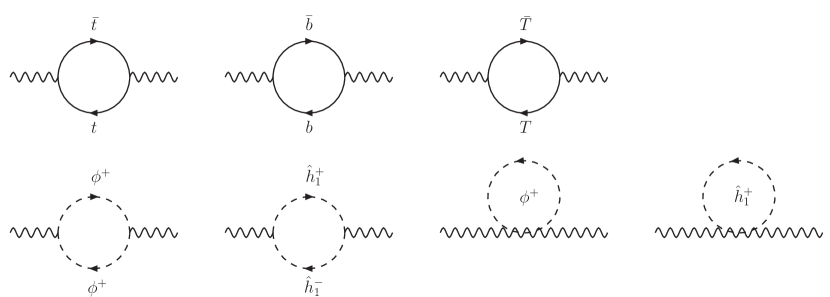
The one-loop corrections to the self-energy $\Pi^{\gamma\gamma}$ of the LRTH model are shown in Figure 7. The total contribution to the self-energy is

$$\Pi^{\gamma\gamma^{\prime}}(0)=\frac{\alpha}{4\pi}\Big{[}\frac{16}{9}\ln\frac{Q^{2}}{m^{2}_{t}}+\frac{4}{9}\ln\frac{Q^{2}}{m^{2}_{b}}+\frac{16}{9}\ln\frac{Q^{2}}{m^{2}_{T}}+\frac{1}{3}\ln\frac{Q^{2}}{m^{2}_{\phi^{+}}}+\frac{1}{3}\ln\frac{Q^{2}}{m^{2}_{\hat{h}_{1}}}+\frac{14}{3\hat{\epsilon}}\Big{]}.$$ (74)

Figure 7: The one-loop corrections to the self-energy $\Pi^{\gamma\gamma}$.

C.2 Contributions to $\Pi^{\gamma Z}(M^{2}_{Z})$

The one-loop corrections to the self-energy $\Pi^{\gamma Z}(M^{2}_{Z})$ are shown in Figure 8. These are (i) fermionic loops having $(\bar{t}t),(\bar{T}T)$ and $(\bar{b}b)$, (ii) the scalar loops due to $SSV$ coupling, $(\phi^{+}\phi^{-})$, $(\hat{h}^{+}_{1}\hat{h}^{-}_{1})$, and (iii) the $\phi^{+}$ and $\hat{h}^{+}_{1}$ scalar loops due to $SSVV$ quartic couplings. The contributions to $\Pi^{\gamma Z}(M^{2}_{Z})$ due to the fermion loops through the couplings in Table 1 are

$$\Pi^{\gamma Z}_{\bar{t}t}(M^{2}_{Z}) =\frac{N_{c}\alpha}{\pi}\frac{2}{3s_{w}c_{w}}\Big{(}\frac{1}{4}C^{2}_{L}-\frac{2}{3}s^{2}_{w}\Big{)}M^{2}_{Z}\Big{[}\frac{1}{3}\Big{(}\ln\frac{Q^{2}}{m^{2}_{t}}+\frac{1}{\hat{\epsilon}}\Big{)}-2I_{3}\Big{(}\frac{M^{2}_{Z}}{m^{2}_{t}}\Big{)}\Big{]},$$ (75)

$$\Pi^{\gamma Z}_{\bar{T}T}(M^{2}_{Z}) =\frac{N_{c}\alpha}{\pi}\frac{2}{3s_{w}c_{w}}\Big{(}\frac{1}{4}S^{2}_{L}-\frac{2}{3}s^{2}_{w}\Big{)}M^{2}_{Z}\Big{[}\frac{1}{3}\Big{(}\ln\frac{Q^{2}}{m^{2}_{T}}+\frac{1}{\hat{\epsilon}}\Big{)}-2I_{3}\Big{(}\frac{M^{2}_{Z}}{m^{2}_{T}}\Big{)}\Big{]},$$ (76)

$$\Pi^{\gamma Z}_{\bar{b}b}(M^{2}_{Z}) =\frac{N_{c}\alpha}{4\pi}\frac{1}{3s_{w}c_{w}}\Big{(}\frac{1}{2}-\frac{2}{3}s^{2}_{w}\Big{)}M^{2}_{Z}\Big{[}\frac{1}{3}\Big{(}\ln\frac{Q^{2}}{m^{2}_{b}}+\frac{1}{\hat{\epsilon}}\Big{)}-2I_{3}\Big{(}\frac{M^{2}_{Z}}{m^{2}_{b}}\Big{)}\Big{]}.$$ (77)

The contributions to $\Pi^{\gamma Z}(M^{2}_{Z})$ from the scalar loops through the couplings in Table 2 are

$$\Pi^{\gamma Z}_{\hat{h}_{1}\hat{h}_{1}}(M^{2}_{Z}) =-\frac{\alpha}{4\pi}\frac{c2^{2}_{w}}{c_{w}s_{w}}\Big{[}\Big{(}M^{2}_{\hat{h}_{1}}-\frac{1}{6}M^{2}_{Z}\Big{)}\Big{(}\ln\frac{Q^{2}}{M^{2}_{\hat{h}_{1}}}+\frac{1}{\hat{\epsilon}}\Big{)}$$

$$\qquad+\Big{(}\frac{1}{6}M^{2}_{Z}-\frac{2}{3}M^{2}_{\hat{h}_{1}}\Big{)}I_{1}\Big{(}\frac{M^{2}_{Z}}{M^{2}_{\hat{h}_{1}}}\Big{)}+M^{2}_{\hat{h}_{1}}-\frac{1}{9}M^{2}_{Z}\Big{]},$$ (78)

$$\Pi^{\gamma Z}_{\phi^{+}\phi^{-}}(M^{2}_{Z}) =\frac{\alpha}{2\pi}\frac{s_{w}}{c_{w}}\Big{[}\Big{(}M^{2}_{\phi^{+}}-\frac{1}{6}M^{2}_{Z}\Big{)}\Big{(}\ln\frac{Q^{2}}{M^{2}_{\phi^{+}}}+\frac{1}{\hat{\epsilon}}\Big{)}$$

$$\qquad+\Big{(}\frac{1}{6}M^{2}_{Z}-\frac{2}{3}M^{2}_{\phi^{+}}\Big{)}I_{1}\Big{(}\frac{M^{2}_{Z}}{M^{2}_{\phi^{+}}}\Big{)}+M^{2}_{\phi^{+}}-\frac{1}{9}M^{2}_{Z}\Big{]}.$$ (79)

The contributions to $\Pi^{\gamma Z}(M^{2}_{Z})$ from the scalar loops through the couplings in Table 3 are

$$\Pi^{\gamma Z}_{\hat{h}_{1}\hat{h}_{1}}(M^{2}_{Z}) =\frac{\alpha}{4\pi}\frac{c2^{2}_{w}}{c_{w}s_{w}}\Big{[}1+\ln\frac{Q^{2}}{M^{2}_{\hat{h}_{1}}}+\frac{1}{\hat{\epsilon}}\Big{]}M^{2}_{\hat{h}_{1}},$$ (80)

$$\Pi^{\gamma Z}_{\phi^{+}\phi^{-}}(M^{2}_{Z}) =-\frac{\alpha}{2\pi}\frac{s_{w}}{c_{w}}\Big{[}1+\ln\frac{Q^{2}}{M^{2}_{\phi^{+}}}+\frac{1}{\hat{\epsilon}}\Big{]}M^{2}_{\phi^{+}}.$$ (81)

The terms proportional to $M^{2}_{\hat{h}_{1}}$ and $M^{2}_{\hat{h}_{1}}\ln(Q^{2}/M^{2}_{\hat{h}_{1}})$ in Eq. (78) and (80) cancel between themselves and so do the terms proportional to $M^{2}_{\phi^{+}}$ and $M^{2}_{\phi^{+}}\ln(Q^{2}/M^{2}_{\phi^{+}})$ in Eq. (79) and (81). For $p^{2}=0$, it can be easily checked that the total fermionic and scalar contributions vanish individually. As expected in the unitary gauge no mixing between the two gauge bosons takes place at one-loop due to

$$\Pi^{\gamma Z}(0)=0.$$ (82)

Figure 8: The one-loop corrections to the self-energy $\Pi^{\gamma Z}$.

C.3 Contributions to $\Pi^{WW}(0)$

The contributions to $\Pi^{WW}(0)$ from the fermion loops through the couplings in Table 1 are given as follows,

$$\Pi^{WW}_{\bar{t}b}(0) =\frac{N_{c}\alpha}{4\pi}\frac{C^{2}_{L}}{2s^{2}_{w}}f_{1}(m^{2}_{t},m^{2}_{b}),$$ (83)

$$\Pi^{WW}_{\bar{T}b}(0) =\frac{N_{c}\alpha}{4\pi}\frac{S^{2}_{L}}{2s^{2}_{w}}f_{1}(m^{2}_{T},m^{2}_{b}),$$ (84)

where $1/\hat{\epsilon}$ terms are omitted, and $f_{1}(m^{2}_{1},m^{2}_{2})$ is defined as

$$f_{1}(m^{2}_{1},m^{2}_{2})=\frac{1}{2}(m^{2}_{1}+m^{2}_{2})+\frac{m^{4}_{1}}{m^{2}_{1}-m^{2}_{2}}\ln\frac{Q^{2}}{m^{2}_{1}}-\frac{m^{4}_{2}}{m^{2}_{1}-m^{2}_{2}}\ln\frac{Q^{2}}{m^{2}_{2}}.$$ (85)

The contributions to $\Pi^{WW}(0)$ from the scalar loops through the couplings in Table 3 are given as,

$$\Pi^{WW}_{h}(0) =\frac{\alpha}{16\pi}\frac{1}{s^{2}_{w}}\big{[}1+\ln\frac{Q^{2}}{M^{2}_{h}}+\frac{1}{\hat{\epsilon}}\big{]}M^{2}_{h},$$ (86)

$$\Pi^{WW}_{\hat{h}_{1}^{+}}(0) =\frac{\alpha}{8\pi}\frac{1}{s^{2}_{w}}\big{[}1+\ln\frac{Q^{2}}{M^{2}_{\hat{h}_{1}}}+\frac{1}{\hat{\epsilon}}\big{]}M^{2}_{\hat{h}_{1}},$$ (87)

$$\Pi^{WW}_{\hat{h}_{2}^{0}}(0) =\frac{\alpha}{16\pi}\frac{1}{s^{2}_{w}}\big{[}1+\ln\frac{Q^{2}}{M^{2}_{\hat{h}_{2}}}+\frac{1}{\hat{\epsilon}}\big{]}M^{2}_{\hat{h}_{2}},$$ (88)

$$\Pi^{WW}_{\phi^{+}}(0) =-\frac{\alpha}{24\pi}\frac{x^{2}}{s^{2}_{w}}\big{[}1+\ln\frac{Q^{2}}{M^{2}_{\phi^{+}}}+\frac{1}{\hat{\epsilon}}\big{]}M^{2}_{\phi^{+}},$$ (89)

$$\Pi^{WW}_{\phi^{0}}(0) =-\frac{\alpha}{432\pi}\frac{x^{2}}{s^{2}_{w}}\big{[}1+\ln\frac{Q^{2}}{M^{2}_{\phi^{0}}}+\frac{1}{\hat{\epsilon}}\big{]}M^{2}_{\phi^{0}}.$$ (90)

Note that $\Pi^{WW}_{\phi^{+}}$ and $\Pi^{WW}_{\phi^{0}}$ are much smaller than the other contributions due to the suppression factor $x^{2}$.

Figure 9: The one-loop corrections to the self-energy $\Pi^{WW}$.

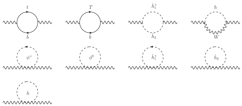
The contribution to $\Pi^{WW}(0)$ from the scalar loops through the couplings in Table 2 has the following form

$$\Pi^{WW}_{\hat{h}_{1}\hat{h}_{2}}(0)=-\frac{\alpha}{2\pi}\frac{1}{s^{2}_{w}}g_{1}(M^{2}_{\hat{h}_{1}},M^{2}_{\hat{h}_{2}}),$$ (91)

where $g_{1}(m^{2}_{1},m^{2}_{2})$ is defined as

$$g_{1}(m^{2}_{1},m^{2}_{2})=\frac{3}{8}(m^{2}_{1}+m^{2}_{2})+\frac{1}{4(m^{2}_{1}-m^{2}_{2})}\big{[}m^{4}_{1}\ln\frac{Q^{2}}{m^{2}_{1}}-m^{4}_{2}\ln\frac{Q^{2}}{m^{2}_{2}}\Big{]}.$$ (92)

The terms proportional to $M^{2}_{\hat{h}_{1}}$ and $M^{2}_{\hat{h}_{1}}\ln(Q^{2}/M^{2}_{\hat{h}_{1}})$ in Eq. (87) and (91) cancel partially between themselves and so do the terms proportional to $M^{2}_{\hat{h}_{2}}$ and $M^{2}_{\hat{h}_{2}}\ln(Q^{2}/M^{2}_{\hat{h}_{2}})$ in Eq. (88) and (91). Although the terms proportional to $M^{2}_{\phi^{+,0}}$ and $M^{2}_{\phi^{+,0}}\ln(Q^{2}/M^{2}_{\phi^{+,0}})$ in Eq. (89) and (90) do not cancel out, their coefficients are significantly small and so are their contributions to $\Pi^{WW}(0)$.

The contribution to $\Pi^{WW}(0)$ from the SM Higgs-W boson loops has the following form

$$\Pi^{WW}_{hW}(0) =\frac{\alpha}{4\pi}\frac{M^{2}_{W}}{s^{2}_{w}}\big{[}\frac{5}{8}-\frac{3}{8}\frac{M^{2}_{h}}{M^{2}_{W}}+\frac{3}{4}\frac{M^{2}_{h}}{M^{2}_{W}-M^{2}_{h}}\ln\frac{Q^{2}}{M^{2}_{W}}$$

$$+\frac{M^{2}_{h}}{M^{2}_{W}-M^{2}_{h}}(-1+\frac{M^{2}_{h}}{M^{2}_{W}})\ln\frac{Q^{2}}{M^{2}_{h}}+(1-\frac{M^{2}_{W}+M^{2}_{h}}{4M^{2}_{W}})\frac{1}{\hat{\epsilon}}\big{]}.$$ (93)

We take only the contribution proportional to $\ln(M^{2}_{S})/16\pi^{2}$, which is gauge invariant,

$$\Pi^{WW}_{hW}(0)=\frac{\alpha}{4\pi}\frac{M^{2}_{W}}{s^{2}_{w}}\ln\frac{Q^{2}}{M^{2}_{h}}\Big{[}\frac{M^{2}_{h}}{M^{2}_{W}-M^{2}_{h}}(-1+\frac{M^{2}_{h}}{M^{2}_{W}})\Big{]}.$$ (94)

C.4 Contributions to $\Pi^{ZZ}(M^{2}_{Z})$

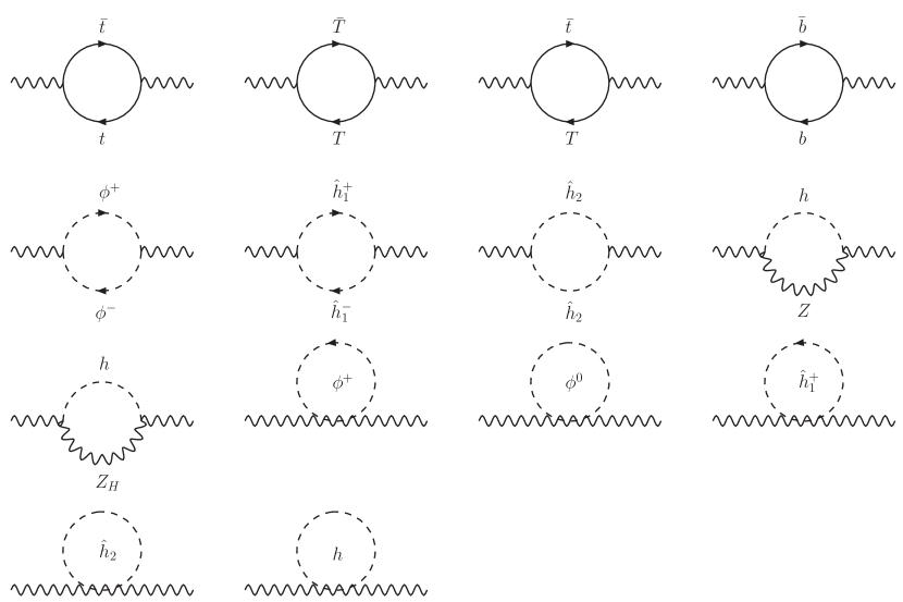
The one-loop corrections to the self-energy function $\Pi^{ZZ}(p^{2})$ are shown in Figure 10. The complete list of fermionic contributions to the self-energy function are given below.

$$\Pi^{ZZ}_{(\bar{T}t)}(M^{2}_{Z}) =\frac{N_{c}\alpha}{4\pi}\frac{1}{c^{2}_{w}}\Big{[}\frac{C_{L}^{2}S_{L}^{2}}{s^{2}_{w}}+\frac{C_{R}^{2}S_{R}^{2}f^{4}x^{4}}{\hat{f}^{4}c^{4}_{w}}\Big{]}\Big{[}\Big{(}\frac{1}{\hat{\epsilon}}+\ln\frac{Q^{2}}{m^{2}_{t}}\Big{)}\Big{(}\frac{M^{2}_{Z}}{6}-\frac{m^{2}_{t}+m^{2}_{T}}{4}\Big{)}$$

$$\quad-M^{2}_{Z}I_{7}\Big{(}\frac{m^{2}_{T}}{m^{2}_{t}},\frac{M^{2}_{Z}}{m^{2}_{t}}\Big{)}-\frac{m^{2}_{T}}{2}I_{5}\Big{(}\frac{m^{2}_{T}}{m^{2}_{t}},\frac{M^{2}_{Z}}{m^{2}_{t}}\Big{)}-\frac{m^{2}_{t}}{2}I_{6}\Big{(}\frac{m^{2}_{T}}{m^{2}_{t}},\frac{M^{2}_{Z}}{m^{2}_{t}}\Big{)}\Big{]}$$

$$\quad+\frac{N_{c}\alpha}{8\pi}\frac{C_{L}S_{L}C_{R}S_{R}}{c_{w}^{4}}\frac{x^{2}f^{2}}{\hat{f}^{2}}m_{t}m_{T}\Big{[}\frac{1}{\hat{\epsilon}}+\ln\frac{Q^{2}}{m^{2}_{t}}-I_{4}(\frac{m^{2}_{T}}{m^{2}_{t}},\frac{M^{2}_{Z}}{m^{2}_{t}})\Big{]},$$

$$\Pi^{ZZ}_{(\bar{t}T)}(M^{2}_{Z}) =\Pi^{ZZ}_{(\bar{T}t)}(M^{2}_{Z})(m_{t}\leftrightarrow m_{T}),$$ (95)

$$\Pi^{ZZ}_{(\bar{t}t)}(M^{2}_{Z}) =\frac{N_{c}\alpha}{\pi}\frac{1}{c^{2}_{w}s^{2}_{w}}\Big{[}\Big{(}\frac{1}{2}C^{2}_{L}-\frac{2}{3}s^{2}_{w}\Big{)}^{2}+\frac{4}{9}s^{4}_{w}\Big{]}\Big{[}\Big{(}\frac{1}{\hat{\epsilon}}+\ln\frac{Q^{2}}{m^{2}_{t}}\Big{)}\Big{(}\frac{M^{2}_{Z}}{6}-\frac{m^{2}_{t}}{2}\Big{)}$$

$$\quad-M^{2}_{Z}I_{3}\Big{(}\frac{M^{2}_{Z}}{m^{2}_{t}}\Big{)}-\frac{m^{2}_{T}}{2}I_{1}\Big{(}\frac{M^{2}_{Z}}{m^{2}_{t}}\Big{)}\Big{]}$$

$$\quad-\frac{2N_{c}\alpha}{3\pi}\frac{1}{c^{2}_{w}}\Big{(}\frac{1}{2}C^{2}_{L}-\frac{2}{3}s^{2}_{w}\Big{)}m^{2}_{t}\Big{[}\frac{1}{\hat{\epsilon}}+\ln\frac{Q^{2}}{m^{2}_{t}}-I_{1}\Big{(}\frac{M^{2}_{Z}}{m^{2}_{t}}\Big{)}\Big{]},$$ (96)

$$\Pi^{ZZ}_{(\bar{T}T)}(M^{2}_{Z}) =\frac{N_{c}\alpha}{\pi}\frac{1}{c^{2}_{w}s^{2}_{w}}\Big{[}\Big{(}\frac{1}{2}S^{2}_{L}-\frac{2}{3}s^{2}_{w}\Big{)}^{2}+\frac{4}{9}s^{4}_{w}\Big{]}\Big{[}\Big{(}\frac{1}{\hat{\epsilon}}+\ln\frac{Q^{2}}{m^{2}_{T}}\Big{)}\Big{(}\frac{M^{2}_{Z}}{6}-\frac{m^{2}_{T}}{2}\Big{)}$$

$$\quad-M^{2}_{Z}I_{3}\Big{(}\frac{M^{2}_{Z}}{m^{2}_{T}}\Big{)}-\frac{m^{2}_{T}}{2}I_{1}\Big{(}\frac{M^{2}_{Z}}{m^{2}_{T}}\Big{)}\Big{]}$$

$$\quad-\frac{2N_{c}\alpha}{3\pi}\frac{1}{c^{2}_{w}}\Big{(}\frac{1}{2}S^{2}_{L}-\frac{2}{3}s^{2}_{w}\Big{)}m^{2}_{T}\Big{[}\frac{1}{\hat{\epsilon}}+\ln\frac{Q^{2}}{m^{2}_{T}}-I_{1}\Big{(}\frac{M^{2}_{Z}}{m^{2}_{T}}\Big{)}\Big{]},$$ (97)

$$\Pi^{ZZ}_{(\bar{b}b)}(M^{2}_{Z}) =\frac{N_{c}\alpha}{4\pi}\frac{1}{c^{2}_{w}s^{2}_{w}}\Big{[}\Big{(}-1+\frac{2}{3}s^{2}_{w}\Big{)}^{2}+\frac{4}{9}s^{4}_{w}\Big{]}\Big{[}\Big{(}\frac{1}{\hat{\epsilon}}+\ln\frac{Q^{2}}{m^{2}_{b}}\Big{)}\Big{(}\frac{M^{2}_{Z}}{6}-\frac{m^{2}_{b}}{2}\Big{)}$$

$$\quad-M^{2}_{Z}I_{3}\Big{(}\frac{M^{2}_{Z}}{m^{2}_{b}}\Big{)}-\frac{m^{2}_{b}}{2}I_{1}\Big{(}\frac{M^{2}_{Z}}{m^{2}_{b}}\Big{)}\Big{]}$$

$$\quad+\frac{N_{c}\alpha}{6\pi}\frac{1}{c^{2}_{w}}\Big{(}-1+\frac{2}{3}s^{2}_{w}\Big{)}m^{2}_{b}\Big{[}\frac{1}{\hat{\epsilon}}+\ln\frac{Q^{2}}{m^{2}_{b}}-I_{1}\Big{(}\frac{M^{2}_{Z}}{m^{2}_{b}}\Big{)}\Big{]}.$$ (98)

The contributions to $\Pi^{ZZ}(M^{2}_{Z})$ from the scalar loops through the couplings in Table 3 have the following form,

$$\Pi^{ZZ}_{(h)}(M^{2}_{Z}) =\frac{\alpha}{16\pi}\frac{1}{c^{2}_{w}s^{2}_{w}}M^{2}_{h}\Big{[}1+\ln\frac{Q^{2}}{M^{2}_{h}}+\frac{1}{\hat{\epsilon}}\Big{]},$$ (99)

$$\Pi^{ZZ}_{(\hat{h}_{1})}(M^{2}_{Z}) =\frac{\alpha}{8\pi}\frac{c2^{4}_{w}}{c^{2}_{w}s^{2}_{w}}M^{2}_{\hat{h}_{1}}\Big{[}1+\ln\frac{Q^{2}}{M^{2}_{\hat{h}_{1}}}+\frac{1}{\hat{\epsilon}}\Big{]},$$ (100)

$$\Pi^{ZZ}_{(\hat{h}_{2})}(M^{2}_{Z}) =\frac{\alpha}{8\pi}\frac{1}{c^{2}_{w}s^{2}_{w}}M^{2}_{\hat{h}_{2}}\Big{[}1+\ln\frac{Q^{2}}{M^{2}_{\hat{h}_{2}}}+\frac{1}{\hat{\epsilon}}\Big{]},$$ (101)

$$\Pi^{ZZ}_{(\phi^{+})}(M^{2}_{Z}) =\frac{\alpha}{2\pi}\frac{s^{2}_{w}}{c^{2}_{w}}M^{2}_{\phi^{+}}\Big{[}1+\ln\frac{Q^{2}}{M^{2}_{\phi^{+}}}+\frac{1}{\hat{\epsilon}}\Big{]},$$ (102)

$$\Pi^{ZZ}_{(\phi^{0})}(M^{2}_{Z}) =-\frac{\alpha}{8\pi}\frac{x^{2}}{54c^{2}_{w}s^{2}_{w}}M^{2}_{\phi^{0}}\Big{[}1+\ln\frac{Q^{2}}{M^{2}_{\phi^{0}}}+\frac{1}{\hat{\epsilon}}\Big{]}.$$ (103)

The contributions to $\Pi^{ZZ}(M^{2}_{Z})$ from the scalar loops through the couplings in Table 2 have the following form,

$$\Pi^{ZZ}_{(\hat{h}_{1}^{\dagger}\hat{h}_{1})}(M^{2}_{Z}) =-\frac{\alpha}{8\pi}\frac{c2^{4}_{w}}{c^{2}_{w}s^{2}_{w}}\Big{[}\Big{(}M^{2}_{\hat{h}_{1}}-\frac{1}{6}M^{2}_{Z}\Big{)}\Big{(}\ln\frac{Q^{2}}{M^{2}_{\hat{h}_{1}}}+\frac{1}{\hat{\epsilon}}\Big{)}$$

$$\quad+\Big{(}\frac{1}{6}M^{2}_{Z}-\frac{2}{3}M^{2}_{\hat{h}_{1}}\Big{)}I_{1}\Big{(}\frac{M^{2}_{Z}}{M^{2}_{\hat{h}_{1}}}\Big{)}+M^{2}_{\hat{h}_{1}}-\frac{1}{9}M^{2}_{Z}\Big{]},$$ (104)

$$\Pi^{ZZ}_{(\hat{h}_{2}^{\dagger}\hat{h}_{2})}(M^{2}_{Z}) =-\frac{\alpha}{8\pi}\frac{1}{c^{2}_{w}s^{2}_{w}}\Big{[}\Big{(}M^{2}_{\hat{h}_{2}}-\frac{1}{6}M^{2}_{Z}\Big{)}\Big{(}\ln\frac{Q^{2}}{M^{2}_{\hat{h}_{2}}}+\frac{1}{\hat{\epsilon}}\Big{)}$$

$$\quad+\Big{(}\frac{1}{6}M^{2}_{Z}-\frac{2}{3}M^{2}_{\hat{h}_{2}}\Big{)}I_{1}\Big{(}\frac{M^{2}_{Z}}{M^{2}_{\hat{h}_{2}}}\Big{)}+M^{2}_{\hat{h}_{2}}-\frac{1}{9}M^{2}_{Z}\Big{]},$$ (105)

$$\Pi^{ZZ}_{(\phi^{+}\phi^{-})}(M^{2}_{Z}) =-\frac{\alpha}{2\pi}\frac{s^{2}_{w}}{c^{2}_{w}}\Big{[}\Big{(}M^{2}_{\phi^{+}}-\frac{1}{6}M^{2}_{Z}\Big{)}\Big{(}\ln\frac{Q^{2}}{M^{2}_{\phi^{+}}}+\frac{1}{\hat{\epsilon}}\Big{)}$$

$$\quad+\Big{(}\frac{1}{6}M^{2}_{Z}-\frac{2}{3}M^{2}_{\phi^{+}}\Big{)}I_{1}\Big{(}\frac{M^{2}_{Z}}{M^{2}_{\phi^{+}}}\Big{)}+M^{2}_{\phi^{+}}-\frac{1}{9}M^{2}_{Z}\Big{]},$$ (106)

$$\Pi^{ZZ}_{(h\phi^{0})}(M^{2}_{Z}) =0.$$ (107)

The terms proportional to $M^{2}_{\hat{h}_{1}}$ and $M^{2}_{\hat{h}_{1}}\ln(Q^{2}/M^{2}_{\hat{h}_{1}})$ in Eq. (100) and (104) cancel between themselves and so do the terms proportional to $M^{2}_{\hat{h}_{2}}$ and $M^{2}_{\hat{h}_{2}}\ln(Q^{2}/M^{2}_{\hat{h}_{2}})$ in Eq. (101) and (105). The terms proportional to $M^{2}_{\phi^{+}}$ and $M^{2}_{\phi^{+}}\ln(Q^{2}/M^{2}_{\phi^{+}})$ in Eq. (102) and (106) also cancel between themselves.

There are contributions of scalar-gauge boson loops to $\Pi^{ZZ}(M^{2}_{Z})$. We take only the contribution proportional to $\ln(M^{2}_{S})/16\pi^{2}$, which is gauge invariant,

$$\Pi^{ZZ}_{(Zh)}(M^{2}_{Z}) =\frac{\alpha}{8\pi}\frac{M^{2}_{W}}{c^{4}_{w}s^{2}_{w}}\ln\frac{Q^{2}}{M^{2}_{h}}\Big{[}1-\frac{3M^{2}_{h}+2M^{2}_{Z}}{12M^{2}_{Z}}\Big{]},$$ (108)

$$\Pi^{ZZ}_{(Z_{H}h)}(M^{2}_{Z}) =\frac{\alpha}{16\pi}\frac{f^{2}x^{2}}{c^{4}_{w}c2^{2}_{w}}\ln\frac{Q^{2}}{M^{2}_{h}}\Big{[}1-\frac{3M^{2}_{h}+3M^{2}_{Z_{H}}-M^{2}_{Z}}{12M^{2}_{Z_{H}}}\Big{]}.$$ (109)

Figure 10: The one-loop corrections to the self-energy function $\Pi^{ZZ}$.

References

- (1) H. Georgi and A. Pais, Phys. Rev. D 10 (1974) 539.
- (2) D. B. Kaplan and H. Georgi, Phys. Lett. B 136 (1984) 183.
- (3) N. Arkani-Hamed, A. G. Cohen and H. Georgi, Phys. Lett. B 513 (2001) 232 [arXiv:hep-ph/0105239].
- (4) N. Arkani-Hamed, A. G. Cohen, T. Gregoire and J. G. Wacker, JHEP 0208 (2002) 020 [arXiv:hep-ph/0202089].
- (5) N. Arkani-Hamed, A. G. Cohen, E. Katz, A. E. Nelson, T. Gregoire and J. G. Wacker, JHEP 0208 (2002) 021 [arXiv:hep-ph/0206020].
- (6) N. Arkani-Hamed, A. G. Cohen, E. Katz and A. E. Nelson, JHEP 0207 (2002) 034 [arXiv:hep-ph/0206021].
- (7) M. Schmaltz, Nucl. Phys. Proc. Suppl. 117 (2003) 40 [arXiv:hep-ph/0210415].
- (8) Z. Chacko, H. S. Goh and R. Harnik, Phys. Rev. Lett. 96 (2006) 231802 [arXiv:hep-ph/0506256].
- (9) Z. Chacko, H. S. Goh and R. Harnik, JHEP 0601 (2006) 108 [arXiv:hep-ph/0512088].
- (10) H. -S. Goh and S. Su, Phys. Rev. D 75 (2007) 075010 [hep-ph/0611015].
- (11) M. C. Chen and S. Dawson, Phys. Rev. D 70 (2004) 015003 [arXiv:hep-ph/0311032].
- (12) A. Sirlin, Phys. Rev. D 22 (1980) 971.
- (13) T. Blank and W. Hollik, Nucl. Phys. B 514 (1998) 113 [arXiv:hep-ph/9703392].
- (14) W. M. Yao et al. [Particle Data Group], J. Phys. G 33 (2006) 1.
- (15) [ALEPH Collaboration], Phys. Rept. 427 (2006) 257 [arXiv:hep-ex/0509008].
- (16) G. Rodrigo, A. Santamaria and M. S. Bilenky, Phys. Rev. Lett. 79 (1997) 193 [arXiv:hep-ph/9703358].
- (17) T. Han, H. E. Logan, B. McElrath and L. T. Wang, Phys. Rev. D 67 (2003) 095004 [arXiv:hep-ph/0301040].
- (18) G. Passarino and M. J. G. Veltman, Nucl. Phys. B 160 (1979) 151.
- (19) G. Degrassi and A. Sirlin, Phys. Rev. D 46 (1992) 3104.
- (20) A. Denner, G. Weiglein and S. Dittmaier, Phys. Lett. B 333 (1994) 420 [arXiv:hep-ph/9406204].
- (21) G. Beall, M. Bander and A. Soni, Phys. Rev. Lett. 48 (1982) 848.
- (22) A. A. Affolder et al. [CDF Collaboration], Phys. Rev. Lett. 87 (2001) 231803 [arXiv:hep-ex/0107008].
- (23) S. Abachi et al. [D0 Collaboration], Phys. Rev. Lett. 76 (1996) 3271 [arXiv:hep-ex/9512007].
- (24) R. Barate et al. [LEP Working Group for Higgs boson searches], Phys. Lett. B 565 (2003) 61 [arXiv:hep-ex/0306033].