Electroweak constraints on warped models with custodial symmetry.

Abstract

It has been recently argued that realistic models with warped extra dimensions can have Kaluza-Klein particles accessible at the Large Hadron Collider if a custodial symmetry, $SU(2)_{V}\times P_{LR}$, is used to protect the $T$ parameter and the coupling of the left-handed bottom quark to the $Z$ gauge boson. In this article we emphasize that such a symmetry implies that the loop corrections to both the $T$ parameter and the $Zb_{L}\bar{b}_{L}$ coupling are calculable. In general, these corrections are correlated, can be sizable, and should be considered to determine the allowed parameter space region in models with warped extra dimensions and custodial symmetry, including Randall-Sundrum models with a fundamental Higgs, models of gauge-Higgs unification and Higgsless models. As an example, we derive the constraints that arise on a representative model of gauge-Higgs unification from a global fit to the precision electroweak observables. A scan over the parameter space typically leads to a lower bound on the Kaluza-Klein excitations of the gauge bosons of about $2-3$ TeV, depending on the configuration. In the fermionic sector one can have Kaluza-Klein excitations with masses of a few hundred GeV. We present the constraints on these light fermions from recent Tevatron searches, and explore interesting discovery channels at the LHC.

I Introduction

Models with warped extra dimensions Randall:1999ee represent a very exciting alternative to more traditional extensions of the Standard Model (SM), like supersymmetry. These models provide not only a natural solution to the hierarchy problem, but also a very compelling theory of flavor, when fermions are allowed to propagate in the bulk Grossman:1999ra . The large hierarchies among the different fermion masses arise in a natural way, without inducing new sources of flavor violation for the first and second generation fermions. On the the other hand, large flavor violation effects are predicted for the third generation fermions, most notably for the top quark Gherghetta:2000qt . It has been recently realized that an enlarged bulk gauge symmetry,

$$SU(2)_{L}\times SU(2)_{R}\times U(1)_{X}~{},$$ (1)

can act as a custodial symmetry that protects two of the most constraining observables from large tree-level corrections: the Peskin-Takeuchi Peskin:1991sw $T$ parameter Agashe:2003zs and, if an extra discrete left-right symmetry $P_{LR}$ is imposed, the anomalous $Zb_{L}\bar{b}_{L}$ coupling Agashe:2006at . When the zero modes of the first two generations are localized far from the IR brane, so as to explain the low-energy flavor structure, an analysis of the electroweak (EW) precision data based on the oblique corrections parametrized by $S$ and $T$, together with the heavy flavor asymmetries and branching ratios, takes into account the most important effects. Therefore, at tree level, the custodial protection of the $T$ parameter and the $Zb_{L}\bar{b}_{L}$ coupling leaves the $S$ parameter as the only relevant constraint.

However, as emphasized in Carena:2006bn , there are calculable one-loop corrections to the precision electroweak observables, which can be relevant and should be taken into account. In fact, for the choice of quantum numbers that lead to the custodial protection of the $Zb_{L}\bar{b}_{L}$ coupling, it was shown that the contribution of these loop corrections yields tight constraints on the parameters of these models, which in turn can have interesting implications for the spectrum of Kaluza-Klein (KK) states and their phenomenology.

In Ref. Carena:2006bn we performed an analysis of the constraints from precision electroweak observables, including one-loop effects, for a specific model based on gauge-Higgs unification, when the light fermions are localized near the UV brane. We obtained a bound on the mass of the first level KK excitations of the gauge bosons of about $3$-$4$ TeV, together with light KK quarks with masses of order of a few hundred GeV, some of them with exotic electric charges. Since the $S$ parameter yields one of the most relevant constraints in these models, one would like to investigate whether scenarios with the light generation fermions localized near the conformal point (flat wavefunctions for the zero-modes), where the couplings of these fermions to the $SU(2)_{L}$ KK modes are suppressed, can lead to a better fit Cacciapaglia:2004rb . Generically, however, an analysis based on the oblique approximation is not sufficient in this region, since the couplings of fermions to $SU(2)_{R}$ gauge bosons tend to induce anomalous, nonuniversal couplings to the $W$ and $Z$ gauge bosons.

It is important to emphasize that, due to the custodial symmetry, the corrections to the $T$ parameter and the $Zb_{L}\bar{b}_{L}$ vertex cannot receive contributions from higher dimension 5D operators suppressed by a low cutoff scale and are, therefore, calculable. In addition, in any given model these two quantities satisfy a definite correlation which, in general, may be understood in terms of the contribution of the lightest KK modes. The potentially large loop corrections to the $T$ parameter and the $Zb_{L}\bar{b}_{L}$ coupling, as well as the effects of the associated correlations, must be considered in any model that makes use of the custodial symmetry. This includes models of gauge-Higgs unification gauge:Higgs:unification ; Contino:2003ve ; Agashe:2004rs and models with a fundamental Higgs or even without a Higgs Cacciapaglia:2006gp .

In this work, we present the results of a global fit to all relevant EW precision observables, taking into account the correlations among them as well as possible non-universal effects, in a particular setting. We have chosen to test these ideas in the context of gauge-Higgs unification scenarios, which we find particularly well motivated theoretically since they address the little hierarchy problem present in Randall-Sundrum models with a fundamental Higgs. In addition, this framework naturally leads to light KK fermion states, often with exotic charges, that makes these scenarios quite interesting from a phenomenological point of view.

The outline of the paper is as follows. We introduce the model in Section II and discuss its main effects on EW observables in Section III. The results of the global fit are reported in Section IV and we discuss some simple variations in section V. In Section VI we present an interesting example which allows for light KK fermions for the three generations within the reach of present and near future colliders. We discuss the bounds from EW precision observables in combination with those from direct searches at the Tevatron. We also discuss interesting search channels at the LHC. Finally we conclude in section VII. Some technical results are given in the Appendix.

II A Model of Gauge-Higgs Unification

Our setup is a 5-dimensional model in a warped background,

$$ds^{2}=e^{-2ky}\eta_{\mu\nu}dx^{\mu}dx^{\nu}-dy^{2}~{},$$ (2)

where $0\leq y\leq L$. The bulk gauge symmetry is $SO(5)\times U(1)_{X}$, broken by boundary conditions to $SU(2)_{L}\times SU(2)_{R}\times U(1)_{X}$ on the IR brane ($y=L$), and to the Standard Model $SU(2)_{L}\times U(1)_{Y}$ gauge group on the UV brane ($y=0$) Agashe:2004rs . The $U(1)_{X}$ charges are adjusted so as to recover the correct hypercharges, where $Y/2=T^{3}_{R}+Q_{X}$ with $T^{3}_{R}$ the third $SU(2)_{R}$ generator and $Q_{X}$ the $U(1)_{X}$ charge. The fifth component of the gauge fields in $SO(5)/SU(2)_{L}\times SU(2)_{R}$ has a (four-dimensional scalar) zero mode with the quantum numbers of the Higgs boson. This zero mode has a non-trivial profile in the extra dimension Contino:2003ve ,

$$A^{\hat{a}}_{5}(x,y)=A^{\hat{a}(0)}_{5}(x)f_{H}(y)+\ldots~{},$$ (3)

where $\hat{a}$ labels the generators of $SO(5)/SU(2)_{L}\times SU(2)_{R}$, and is exponentially localized towards the IR brane

$$f_{H}(y)=\sqrt{\frac{2k}{e^{2kL}-1}}\,e^{2ky}~{},$$ (4)

hence giving a solution to the hierarchy problem. The dots in Eq. (3) stand for massive KK modes that are eaten by the corresponding KK gauge fields.

The SM fermions are embedded in full representations of the bulk gauge group. The presence of the $SU(2)_{R}$ subgroup of the full bulk gauge symmetry ensures the custodial protection of the $T$ parameter Agashe:2003zs . In order to have a custodial protection of the $Zb_{L}\bar{b}_{L}$ coupling, the choice $T^{3}_{R}(b_{L})=T^{3}_{L}(b_{L})$ has to be enforced Agashe:2006at . An economical choice is to let the SM $SU(2)_{L}$ top-bottom doublet arise from a ${\bf 5}_{2/3}$ of $SO(5)\times U(1)_{X}$, where the subscript refers to the $U(1)_{X}$ charge. As discussed in Carena:2006bn , putting the SM $SU(2)_{L}$ singlet top in the same $SO(5)$ multiplet as the doublet, without further mixing, is disfavored since, for the correct value of the top quark mass, this leads to a large negative contribution to the $T$ parameter at one loop. Hence we let the right-handed top quark arise from a second ${\bf 5}_{2/3}$ of $SO(5)\times U(1)_{X}$. The right handed bottom can come from a ${\bf 10}_{2/3}$ that allows to write the bottom Yukawa coupling. For simplicity, and because it allows the generation of the CKM mixing matrix, we make the same choice for the first two quark generations. We therefore introduce in the quark sector three $SO(5)$ multiplets per generation as follows:

$$\begin{array}[]{c}\begin{array}[]{ccccccc}\xi^{i}_{1L}&\sim&Q^{i}_{1L}&=&\begin{pmatrix}\chi^{u_{i}}_{1L}(-,+)&q^{u_{i}}_{L}(+,+)\\ \chi^{d_{i}}_{1L}(-,+)&q^{d_{i}}_{L}(+,+)\end{pmatrix}&\oplus&u^{\prime i}_{L}(-,+)~{},\vspace{3mm}\\ \xi^{i}_{2R}&\sim&Q^{i}_{2R}&=&\begin{pmatrix}\chi^{u_{i}}_{2R}(+,-)&q^{\prime{u_{i}}}_{R}(+,-)\\ \chi^{d_{i}}_{2R}(+,-)&q^{\prime{d_{i}}}_{R}(+,-)\end{pmatrix}&\oplus&u^{i}_{R}(+,+)~{},\end{array}\vspace{3mm}\\ \begin{array}[]{ccccccccccccc}\xi^{i}_{3R}&\sim&T^{i}_{1R}&=&\begin{pmatrix}\psi^{\prime i}_{R}(-,+)\\ U^{\prime i}_{R}(-,+)\\ D^{\prime i}_{R}(-,+)\end{pmatrix}&\oplus&T^{i}_{2R}&=&\begin{pmatrix}\psi^{\prime\prime i}_{R}(-,+)\\ U^{\prime\prime i}_{R}(-,+)\\ D^{i}_{R}(+,+)\end{pmatrix}&\oplus&Q^{i}_{3R}&=&\begin{pmatrix}\chi^{u_{i}}_{3R}(-,+)&q^{\prime\prime u_{i}}_{R}(-,+)\\ \chi^{d_{i}}_{3R}(-,+)&q^{\prime\prime d_{i}}_{R}(-,+)\end{pmatrix},\end{array}\end{array}$$ (10)

where we show the decomposition under $SU(2)_{L}\times SU(2)_{R}$. The $Q^{i}$’s are bidoublets of $SU(2)_{L}\times SU(2)_{R}$, with $SU(2)_{L}$ acting vertically and $SU(2)_{R}$ acting horizontally. The $T^{i}_{1}$’s and $T^{i}_{2}$’s transform as $({\bf 3},{\bf 1})$ and $({\bf 1},{\bf 3})$ under $SU(2)_{L}\times SU(2)_{R}$, respectively, while $u^{i}$ and $u^{\prime i}$ are $SU(2)_{L}\times SU(2)_{R}$ singlets. The superscripts, $i=1,2,3$, label the three generations.

We also show the boundary conditions on the indicated 4D chirality, where $-$ stands for Dirichlet boundary conditions. The $+$ stands for a linear combination of Neumann and Dirichlet boundary conditions, that is determined via the fermion bulk equations of motion from the Dirichlet boundary condition obeyed by the opposite chirality. In the absence of mixing among multiplets satisfying different boundary conditions, the SM fermions arise as the zero-modes of the fields obeying $(+,+)$ boundary conditions. The remaining boundary conditions are chosen so that $SU(2)_{L}\times SU(2)_{R}$ is preserved on the IR brane, and so that mass mixing terms, necessary to obtain the SM fermion masses after EW symmetry breaking, can be written on the IR brane. It is possible to flip the boundary conditions on $Q^{i}_{2R}$, consistently with these requirements, and we will comment on such a possibility in later sections.

As for the leptons, one option is to embed the SM $SU(2)_{L}$ lepton doublets into the ${\bf 5}_{0}$ representation of $SO(5)\times U(1)_{X}$ and the $SU(2)_{L}$ charged lepton singlets in a ${\bf 10}_{0}$. Right-handed neutrinos may come from the $SU(2)_{L}\times SU(2)_{R}$ singlet in the ${\bf 5}_{0}$, or from a different ${\bf 5}_{0}$, as in the quark sector. The boundary conditions may then be chosen in analogy with those in Eq. (10). A second possibility is that the leptons, unlike the quarks, arise from the 4-dimensional spinorial representation of $SO(5)$, so that the SM lepton doublets transform as $({\bf 2},{\bf 1})$ under $SU(2)_{L}\times SU(2)_{R}$, while the SM lepton singlets transform as $({\bf 1},{\bf 2})$.

As remarked above, the zero-mode fermions can acquire EW symmetry breaking masses through mixing effects. The most general $SU(2)_{L}\times SU(2)_{R}\times U(1)_{X}$ invariant mass Lagrangian at the IR brane –compatible with the boundary conditions– is, in the quark sector,

$$\mathcal{L}_{m}=\delta(y-L)\Big{[}\bar{u}^{\prime}_{L}M_{u}u_{R}+\bar{Q}_{1L}M_{d}Q_{3R}+\bar{Q}_{2L}M_{ud}Q_{3R}+\mathrm{h.c.}\Big{]}~{},$$ (11)

where $M_{u}$, $M_{d}$ and $M_{ud}$ are dimensionless $3\times 3$ matrices, and a matrix notation is employed.

III Effects on Electroweak Observables

In order to study the effects that the KK excitations of bulk fermions and gauge bosons have on EW observables, we compute the effective Lagrangian that results after integrating them out at tree level, keeping the leading corrections with operators of dimension six. As was mentioned in the introduction, some one-loop corrections are also important and will be included on top of the tree-level effects. In fact, in models with custodial protection of the $Zb_{L}\bar{b}_{L}$ coupling, some of the KK fermions become considerably lighter than the KK gauge bosons, and can give relevant loop level effects as a result of their strong mixing with the top quark. The loop contributions to the EW observables coming from the gauge boson KK excitations are suppressed due to their larger masses, as well as to the fact that they couple via the EW gauge couplings, that are smaller than the top Yukawa coupling. Thus we expect their one-loop effects on EW observables to be subleading and we neglect them.

III.1 Tree-level effective Lagrangian

In this section, we compute the effective Lagrangian up to dimension six operators, obtained when the heavy physics in the models discussed in the previous section is integrated out at tree level. We will express the effective Lagrangian in the basis of Buchmuller:1985jz where the dimension six operators are still $SU(2)_{L}\times U(1)_{Y}$ invariant. The procedure is the following. We integrate out the heavy physics in an explicitly $SU(2)_{L}\times U(1)_{Y}$ invariant way and then use the SM equations of motion if necessary to write the resulting operators in the basis of Buchmuller:1985jz . Only a subset of the 81 operators in that basis is relevant for EW precision observables, as discussed in Han:2004az . At the order we are considering, we can integrate out independently each type of heavy physics. The effective Lagrangian in the basis of Buchmuller:1985jz after integrating out the heavy gauge bosons reads

$$\Delta\mathcal{L}_{6} = \alpha_{h}\mathcal{O}_{h}+\alpha^{t}_{hl}\mathcal{O}^{t}_{hl}+\alpha^{t}_{hq}\mathcal{O}^{t}_{hq}+\alpha^{s}_{hl}\mathcal{O}^{s}_{hl}+\alpha^{s}_{hq}\mathcal{O}^{s}_{hq}+\alpha_{hu}\mathcal{O}_{hu}+\alpha_{hd}\mathcal{O}_{hd}+\alpha_{he}\mathcal{O}_{he}$$ (12)

$$+ \alpha^{t}_{ll}\mathcal{O}^{t}_{ll}+\alpha^{t}_{lq}\mathcal{O}^{t}_{lq}+\alpha^{s}_{ll}\mathcal{O}^{s}_{ll}+\alpha^{s}_{lq}\mathcal{O}^{s}_{lq}+\alpha_{le}\mathcal{O}_{le}+\alpha_{qe}\mathcal{O}_{qe}+\alpha_{lu}\mathcal{O}_{lu}+\alpha_{ld}\mathcal{O}_{ld}$$

$$+ \alpha_{ee}\mathcal{O}_{ee}+\alpha_{eu}\mathcal{O}_{eu}+\alpha_{ed}\mathcal{O}_{ed}+\ldots~{},$$

where the dots represent other operators that are irrelevant for the analysis of EW observables. Here $h$ stands for the SM Higgs, $q$ and $l$ refer to the $SU(2)_{L}$ doublet quark and leptons, and $u$, $d$, $e$ refer to the SM $SU(2)_{L}$ quark and lepton singlets. The list of the dimension-six operators generated in our model is:

• Oblique operators

  $$\mathcal{O}_{h}=|h^{\dagger}D_{\mu}h|^{2}~{}.$$ (13)

• Two-fermion operators

  $$\begin{array}[]{cclcccl}\mathcal{O}_{hl}^{s}&=&\mathrm{i}(h^{\dagger}D_{\mu}h)(\bar{l}\gamma^{\mu}l)+\mathrm{h.c.}~{},&&\mathcal{O}_{hl}^{t}&=&\mathrm{i}(h^{\dagger}\sigma^{a}D_{\mu}h)(\bar{l}\gamma^{\mu}\sigma^{a}l)+\mathrm{h.c.}~{},\\ \mathcal{O}_{hq}^{s}&=&\mathrm{i}(h^{\dagger}D_{\mu}h)(\bar{q}\gamma^{\mu}q)+\mathrm{h.c.}~{},&&\mathcal{O}_{hq}^{t}&=&\mathrm{i}(h^{\dagger}\sigma^{a}D_{\mu}h)(\bar{q}\gamma^{\mu}\sigma^{a}q)+\mathrm{h.c.}~{},\\ \mathcal{O}_{hu}&=&\mathrm{i}(h^{\dagger}D_{\mu}h)(\bar{u}\gamma^{\mu}u)+\mathrm{h.c.}~{},&&\mathcal{O}_{hd}&=&\mathrm{i}(h^{\dagger}D_{\mu}h)(\bar{d}\gamma^{\mu}d)+\mathrm{h.c.}~{},\\ \mathcal{O}_{he}&=&\mathrm{i}(h^{\dagger}D_{\mu}h)(\bar{e}\gamma^{\mu}e)+\mathrm{h.c.}~{}.\end{array}$$ (18)

• Four-fermion operators

  $$\begin{array}[]{cclcccl}\mathcal{O}_{ll}^{s}&=&\frac{1}{2}(\bar{l}\gamma^{\mu}l)(\bar{l}\gamma_{\mu}l)~{},&&\mathcal{O}_{ll}^{t}&=&\frac{1}{2}(\bar{l}\gamma^{\mu}\sigma^{a}l)(\bar{l}\gamma_{\mu}\sigma^{a}l)~{},\\ \mathcal{O}_{lq}^{s}&=&(\bar{l}\gamma^{\mu}l)(\bar{q}\gamma_{\mu}q)~{},&&\mathcal{O}_{lq}^{t}&=&(\bar{l}\gamma^{\mu}\sigma^{a}l)(\bar{q}\gamma_{\mu}\sigma^{a}q)~{},\\ \mathcal{O}_{le}&=&(\bar{l}\gamma^{\mu}l)(\bar{e}\gamma_{\mu}e)~{},&&\mathcal{O}_{qe}&=&(\bar{q}\gamma^{\mu}q)(\bar{e}\gamma_{\mu}e)~{},\\ \mathcal{O}_{lu}&=&(\bar{l}\gamma^{\mu}l)(\bar{u}\gamma_{\mu}u)~{},&&\mathcal{O}_{ld}&=&(\bar{l}\gamma^{\mu}l)(\bar{d}\gamma_{\mu}d)~{},\\ \mathcal{O}_{ee}&=&\frac{1}{2}(\bar{e}\gamma^{\mu}e)(\bar{e}\gamma_{\mu}e)~{},\\ \mathcal{O}_{eu}&=&(\bar{e}\gamma^{\mu}e)(\bar{u}\gamma_{\mu}u)~{},&&\mathcal{O}_{ed}&=&(\bar{e}\gamma^{\mu}e)(\bar{d}\gamma_{\mu}d)~{}.\end{array}$$ (25)

The coefficients $\alpha_{i}$ encode the dependence on the different parameters of our model and their explicit form is given in the Appendix.

The heavy fermions can be integrated out in a similar fashion delAguila:2000aa . However their effects are typically negligible for all the SM fermions except for the top quark delAguila:2000kb , whose couplings are irrelevant for the EW precision observables (except for one-loop corrections DelAguila:2001pu that will be considered in the next subsection). We have nevertheless included all these effects numerically. 

The operator $\mathcal{O}_{h}$ gives a direct contribution to the $T$ parameter

$$T=-\frac{4\pi v^{2}}{e^{2}}\alpha_{h}=-\frac{4\pi v^{2}}{c^{2}}[\delta^{2}_{++}-\delta^{2}_{-+}],\$$ (26)

where $\alpha_{h}$ is the coefficient of the corresponding operator as given in the Appendix, $e$ is the positron charge, $c$ is the cosine of the weak mixing angle, $v=174~{}\rm GeV$ is the Higgs vev, and $\delta^{2}_{++}$ and $\delta^{2}_{-+}$ are functions depending on the Higgs and KK gauge boson wavefunctions, as defined in Eq. (54). The (partial) cancellation between $\delta^{2}_{++}$ and $\delta^{2}_{-+}$ in the tree-level contribution to the $T$ parameter of Eq. (26) is a consequence of the custodial symmetry. Also note that the $S$ parameter, generated by the operator

$$\alpha_{WB}\mathcal{O}_{WB}=\alpha_{WB}\,(h^{\dagger}\sigma^{a}h)W^{a}_{\mu\nu}B^{\mu\nu}~{},$$ (27)

where $S=(32\pi sc/e^{2})v^{2}\alpha_{WB}$, is not induced at tree level in our model.

III.2 Large one-loop effects

Although higher dimensional models are nonrenormalizable and many observables receive contributions from higher-dimension operators whose coefficients can only be determined by an unspecified UV completion, it is noteworthy that some of the low-energy observables are actually insensitive to the UV physics. This is the case of the Peskin-Takeuchi $T$ parameter and of the $Zb_{L}\bar{b}_{L}$ coupling in models with custodial symmetry and the quantum numbers used in this paper. In particular, loop contributions to these parameters are dominated by the KK scale. This follows simply from the fact that the assumed symmetries ($SU(2)_{L}\times SU(2)_{R}$ with a discrete symmetry exchanging $L$ with $R$) and quantum number assignments do not allow for local 5D counterterms that can contribute to these observables. Note, however, that one can write operators that contribute to the $Zt_{L}\bar{t}_{L}$ coupling. Although these symmetries are broken by the boundary conditions at the UV brane, such breaking is non-local and effectively leads to finite contributions to the $T$ parameter and the $Zb_{L}\bar{b}_{L}$ coupling at loop level.

The detailed computation of the leading one-loop contributions to the $T$ parameter was first performed in Carena:2006bn . The important observation made in that work is that the presence of bidoublets, necessary to protect the tree-level contribution to the $Zb_{L}\bar{b}_{L}$ coupling, typically induces a negative $T$ parameter at one loop. There are also contributions from the KK excitations of the $SU(2)_{L}\times SU(2)_{R}$ singlets that can alter this result, provided these singlets are relatively light and mix sufficiently strongly with the top quark. In this case, a positive $T$ might be obtained, but also the one-loop contributions to the $Zb_{L}\bar{b}_{L}$ coupling become sizable and therefore relevant for the EW fit.

The main one-loop effects, due to heavy vector-like fermions that mix strongly with the top, can be computed by generalizing the results in Refs.Lavoura:1992np ; Bamert:1996px . We give the detailed formulas in the Appendix, which can be easily evaluated numerically. The largest contributions arise from the KK excitations that couple via the top Yukawa coupling. In the case of the $T$ parameter, the quantitative features can be understood from the following types of contributions:

• A negative contribution to $T$ from the lightest bidoublet excitations that violate the custodial symmetry via the boundary conditions, $Q^{3}_{1}$ in the notation of Eq. (10).

• A positive contribution to $T$ from the lightest $SU(2)_{L}\times SU(2)_{R}$ singlet KK excitations, $u^{\prime 3}$ in the notation of Eq. (10).

In Ref. Carena:2006bn we also gave approximate analytic formulas for the above contributions. The expressions for the bidoublet are somewhat complicated, but the negative contribution arises from the first KK mode of the $(\chi^{u_{3}}_{1},\chi^{d_{3}}_{1})$ $SU(2)_{L}$ doublet, that is lighter and couples more strongly to the Higgs than the lightest KK mode of the $(q^{u_{3}}_{1},q^{d_{3}}_{1})$ $SU(2)_{L}$ doublet (which gives a partially compensating positive contribution). Notice that the contribution due to the $Q^{3}_{2}$ bidoublet is extremely small, even when these modes are very light, since the custodial symmetry is preserved by their boundary conditions. They can give a nonvanishing contribution to $T$ only from mixing with other bidoublets that violate the custodial symmetry. Our choice for the boundary conditions of $Q^{3}_{2}$ is motivated by the desire to forbid a localized mixing mass term between $Q^{3}_{1}$ and $Q^{3}_{2}$, that would make the $(\chi^{u_{3}}_{1},\chi^{d_{3}}_{1})$ KK modes very light and their contribution to the $T$ parameter large and negative (which as we will review below is disfavored by the EW precision data. See also Ref. Carena:2006bn for further details). In the region of parameter space favored by the EW precision data, the boundary conditions for $Q^{3}_{2}$ result in their KK excitations easily being in the few hundred GeV range, and present a very interesting phenomenology (see section VI). It is in the above sense that we regard very light bidoublets as a rather well-motivated signature of the scenarios we are studying.

The positive contribution to $T$ from $u^{\prime 3}$, mentioned above, is simply given by

$$\Delta T=T_{\rm top}\frac{2m^{2}_{q^{t}_{0},t}}{M^{2}_{t}}\left(\ln\frac{M^{2}_{t}}{m^{2}_{\rm top}}-1+\frac{m^{2}_{q^{t}_{0},t}}{2m^{2}_{\rm top}}\right)~{},$$ (28)

where $T_{\rm top}$ is the SM contribution from the top quark, with mass $m_{\rm top}$, $M_{t}$ is the KK mass of $u^{\prime 3}$, and $m_{q^{t}_{0},t}$ is the EW symmetry breaking mass mixing the lightest singlet with the SM $(t,b)$ doublet. There are also terms that arise from the mixing between the first KK modes of the third generation $Q^{3}_{1}$ and $u^{\prime 3}$, that can be relevant.

It is important that the dominant fermion loop contributions to the $Zb_{L}\bar{b}_{L}$ vertex arise from the same set of states as discussed above. The contributions coming from the singlet, $u^{\prime 3}$, are

$$\delta g_{b_{L}}^{s}=\frac{\alpha}{16\pi s^{2}M_{W}^{2}}\frac{m^{4}_{q^{t}_{0},t}}{M_{t}^{2}}\bigg{[}1+2\frac{m^{2}_{\rm top}}{m^{2}_{q^{t}_{0},t}}\Big{(}\ln\left(\frac{M_{t}^{2}}{m^{2}_{\rm top}}\right)-1\Big{)}\bigg{]}~{},$$ (29)

while those coming from $Q^{3}_{1}$ are

$$\delta g_{b_{L}}^{q}+\delta g_{b_{L}}^{\chi}=\frac{\alpha}{32\pi s^{2}M_{W}^{2}}m_{\rm top}^{2}\bigg{[}\frac{m_{q^{t},t}^{2}}{M_{q}^{2}}\ln\left(\frac{M_{q}^{2}}{m_{\rm top}^{2}}\right)-\frac{m_{\chi^{d},t}^{2}}{M_{\chi}^{2}}\ln\left(\frac{M_{\chi}^{2}}{m_{\rm top}^{2}}\right)\bigg{]}~{}.$$ (30)

Here $M_{t}$, $M_{q}$ and $M_{\chi}$ are the KK masses of $u^{\prime 3}$, $q^{u_{3}}_{1}$ and $\chi^{d_{3}}_{1}$, respectively, while $m_{q^{t},t}$ and $m_{\chi^{d},t}$ are the EW breaking masses that mix the right-handed top with the lightest KK modes of the two bidoublet components $q^{u_{3}}_{1}$ and $\chi^{d_{3}}_{1}$, respectively. Also, $M_{W}$ is the $W$ mass, $\alpha$ is the fine structure constant and $s$ is the sine of the weak mixing angle. There are additional contributions from the mixing between bidoublet and singlet KK modes, but we do not give the analytic expressions here since they are somewhat complicated. The dominant contribution arises from the singlet, but the mixing terms can also give a relevant effect.

It should be noted that, although these contributions depend on several mass and mixing parameters, within the context of an extra dimensional theory all of these are highly correlated by the shape of the wavefunctions. As an example, we show in Fig. 1 the correlation between the one-loop contributions to $T$ and the $Zb_{L}\bar{b}_{L}$ vertex in the gauge-Higgs unification scenario based on the $SO(5)\times U(1)_{X}$ gauge symmetry, and with the fermion content given in Eq. (10). In particular, we see that in the region where $T$ becomes positive, the one-loop contribution to the $Zb_{L}\bar{b}_{L}$ vertex increases, and cannot be neglected in the EW fit. In the figure, we did not include the tree-level contributions to the $T$-parameter from gauge KK mode exchange, which are subdominant.

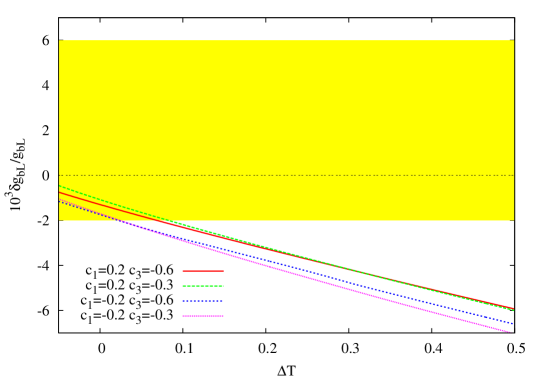
Figure 1: Correlation between the one-loop contributions to the $T$ parameter, denoted by $\Delta T$, and the one-loop contributions to $\delta g_{b_{L}}/g_{b_{L}}$ in the model of Eq. (10). We show representative curves for a few values of the left-handed top quark localization parameter, $c_{1}$, and the bottom quark localization parameter, $c_{3}$, as the right-handed top localization parameter, $c_{2}$, is varied. We take the mass of the first KK excitation of the $SU(2)_{L}$ gauge bosons $m_{1}^{\mathrm{gauge}}=3.75~{}{\rm TeV}$. The band corresponds to the 2-$\sigma$ bound on $\delta g_{bL}/g_{bL}$, assuming no large corrections to the $Zb_{R}\bar{b}_{R}$ coupling.

Given the importance of these one-loop corrections, we have formally added them to the effective Lagrangian at the same level as the tree-level corrections computed in the previous section. This is done by simply adding the corresponding results of Eqs. (A.2-66) to the coefficients of the operators $\mathcal{O}_{h}$ and $\mathcal{O}_{hQ}^{t}$ (here $Q$ represents the doublet of the third generation).

We have also computed the one-loop contributions to the $S$-parameter. Although there is no reason to expect the result to be UV insensitive, one finds that at one loop the sum over KK modes converges fast. In the region of parameter space we are interested, the corresponding contribution to $S$ is not negligible, and we include it as a contribution to the operator $\mathcal{O}_{WB}$ defined in Eq. (27). We take this as a reasonable estimate of the total contribution to $S$, but one should keep in mind that, at least in principle, additional UV contributions to $S$ could have a significant impact. Note that, when the light fermions are localized far from the IR brane, the universal shift in their couplings to the gauge bosons can be reabsorbed as an additional tree-level contribution to the $S$ parameter. Since the tree- and loop-level contributions to the $S$ parameter have the same sign, it is natural to assume that there are no particular cancellations when the effects of the physics above the UV cut-off are included. In particular, the $S$ parameter is positive, thus disfavoring the regions of parameter space that lead to a negative $T$ parameter Yao:2006px .

IV Global fit to Electroweak precision observables

Having computed the leading corrections to the effective Lagrangian in the model of interest, we can compute the $\chi^{2}$ function, defined by

$$\chi^{2}(\alpha_{i}) = \chi^{2}_{\rm min}+(\alpha_{i}-\hat{\alpha}_{i}){\cal M}_{ij}(\alpha_{j}-\hat{\alpha}_{j})~{},$$ (31)

where the $\alpha_{i}$’s, as defined by Eq. (12), depend on the fundamental parameters of the model: localization parameters for each 5D fermion multiplet, $c_{\xi_{i}}$, localized fermion mass mixing parameters, $M_{u}$, $M_{d}$ and $M_{ud}$, as defined in Eq. (11), the gauge couplings, $g_{5}$ and $g_{5\,X}$, and the overall scale of the new physics, which we take as $\tilde{k}=k\,e^{-kL}$. The matrix ${\cal M}_{ij}$ and the vector $\hat{\alpha}_{i}$ are obtained by performing a global fit to the experimental data. We use the fit of Ref. Han:2004az , which takes into account low-energy measurements, as well as the results from LEP1, SLD and LEP2. However, we have not included the NuTeV results.

Although the model contains a large number of parameters, some of these, or certain combinations of them, are fixed by the low-energy gauge couplings, fermion masses and fermion mixing angles. Also, in order to avoid dangerous FCNC’s we have considered family independent localization parameters, $c_{\xi_{1}}^{\mathrm{light}},c_{\xi_{2}}^{\mathrm{light}},c_{\xi_{3}}^{\mathrm{light}}$, for the multiplets giving rise to the light SM fermions. A scan over parameter space shows that the EW fit favors the light right-handed (RH) quarks and leptons to be localized near the UV brane ($c_{\xi_{2}}^{\mathrm{light}}\sim c_{\xi_{3}}^{\mathrm{light}}\sim-0.6$) and the left-handed (LH) quarks and leptons to be localized close to each other. Thus, we will take a common localization parameter for the light LH quarks and leptons, denoted by $c_{\mathrm{light}}$, and, unless otherwise specified, we place the light RH fermions near the UV brane (we denote their localization parameters by $c_{\rm RH}$). Although the assumption of family independence is quite important when the fermions are localized near the IR brane, it is not essential when the fermions are localized closer to the UV brane (the fermion mass hierarchies can then be generated by exponential wavefunction factors). In particular, if the light fermions are localized close to the UV brane, the results of our global fit apply even if their localization parameters are not family universal. As for the third quark family, we have allowed independent localization parameters for the different multiplets: $c_{1}$ for the multiplet giving rise to the $SU(2)_{L}$ doublet $(t,b)_{L}$, $c_{2}$ for the multiplet giving rise to $t_{R}$, and $c_{3}$ for the multiplet giving rise to $b_{R}$.

Regarding the localized mass mixing terms of Eq. (11), when the first two generations are localized near the IR brane, the corresponding terms are extremely small (of order $m_{f}/\tilde{k}$, where $m_{f}$ is a fermion mass), and have a negligible effect. In this case, the only large boundary mass is $M_{u}^{33}$, that is fixed by the top quark mass for each value of $c_{1}$ and $c_{2}$. However, when the light fermions are localized near the UV brane, the mixing mass terms can be of order one (recall these are dimensionless parameters). In this case, they can have an important effect on the KK spectrum. Nevertheless, they still have a negligible effect on the EW fit, for the following reasons. As discussed before, there are potentially important contributions from fermion KK modes both at tree- and loop-level. The tree-level effects arise from mixing, after electroweak symmetry breaking, between the zero-mode and the massive fermion modes, and can affect the couplings to the gauge bosons of the SM fermions. Since the region where the localized masses are of order one corresponds to the case where the zero-mode fermions are far from the IR brane, and since the mixing effects are proportional to the overlap between this wavefunction and the Higgs profile, which is localized near the IR brane, it is easy to see that the relevant mixing angles are exponentially suppressed. On the other hand, when the zero-mode fermions are near the IR brane, the localized masses are forced to be small due to the smallness of the light fermion masses, so that the mixing effects are again suppressed (for the down-type fermions, the custodial symmetry enforces additional cancellations). We have checked that these tree-level effects are always numerically negligible. The second class of potentially large effects arises at loop level. When the zero-mode fermions are near the IR brane, the loop effects are directly proportional to the fourth power of the small localized mixing parameters. When the zero-mode fermions are localized near the UV brane, although the loop contributions involving mixing with the zero mode are exponentially suppressed as above, there are loop contributions involving only mixing among massive KK states, that are not necessarily negligible. However, in this limit the massive KK spectrum is $SO(5)$ symmetric to a very good approximation. As a result, the loop contributions to the $T$ parameter and the $Zb_{L}\bar{b}_{L}$ vertex discussed in the previous section, due to the first two generations, are numerically negligible due to the custodial symmetry. We have also verified that the $S$ parameter has only a weak dependence on the localized mixing masses. Thus, we conclude that for the purpose of the EW fit analysis, the mixing masses involving the light generations can be neglected (although, of course, they are important in reproducing the correct fermion masses and mixing angles). Therefore, we are left with six relevant model parameters: $c_{\mathrm{light}}$, $c_{\rm RH}$, $c_{1}$, $c_{2}$, $c_{3}$ and $\tilde{k}$.

It should be noted that in models of gauge-Higgs unification the Higgs potential –that is induced at loop-level– is also calculable gauge:Higgs:unification . Therefore, given the matter and gauge content of the model, the scale of new physics, $\tilde{k}$, is tied to the scale of EW symmetry breaking by the gauge and Yukawa couplings (the latter ones, as determined by the localized mass parameters). However, it is possible to imagine additional matter content that could affect the Higgs potential without having an impact on the EW precision measurements (e.g. 5D fermion multiplets without zero-modes and with exotic quantum numbers that do not allow mixing with the SM fermions). Therefore, we treat $\tilde{k}$ as an effectively independent parameter. Given the correlation between $\tilde{k}$ and the Higgs vev in any such model, one can use our bounds on $\tilde{k}$ to get an idea of whether the model is excluded or not (however, if $\tilde{k}$ turns out to be too small, an analysis that goes beyond the linear treatment of the Higgs couplings used here might be necessary). On the other hand, our approach allows us to apply our bounds to more general models with a bulk Higgs, and where the Yukawa couplings arise in a similar manner as in gauge-Higgs unification scenarios. We will also assume that, as happens in gauge-Higgs unification scenarios, the Higgs is light, and we have used a Higgs mass $m_{H}=120~{}{\rm GeV}$.

It was shown in Ref. Carena:2006bn that the $T$ parameter in models with custodial protection of the $Zb_{L}\bar{b}_{L}$ vertex is negative and non-negligible in a large region of parameter space. However, it exhibits a strong dependence on the right-handed top localization parameter, $c_{2}$, when the right-handed top has a nearly flat wavefunction, corresponding to $c_{2}\sim-0.5$. In this case, $T$ can easily reach positive values of order one, so that by adjusting $c_{2}$ one can get essentially any value of $T$. Thus, in order to reduce the dimension of our parameter space we have chosen to minimize the $\chi^{2}$ with respect to $c_{2}$ for each value of the rest of the parameters. Note that this also takes into account the loop corrections to the $Zb_{L}\bar{b}_{L}$ vertex, since these are correlated with the $T$ parameter as exemplified in Fig. 1. By taking the RH fermions near the UV brane we are also minimizing with respect to $c_{\rm RH}$. We have therefore performed a four-parameter fit and obtained the $2\sigma$ bound on $\tilde{k}$ by varying the $\chi^{2}$ with respect to the other three parameters, $c_{\mathrm{light}}$, $c_{1}$ and $c_{3}$. The first of these parameters, that determines the localization of the light fermions, affects directly the tree-level effective Lagrangian computed in Section III.1, whereas the latter two, that involve localization of the third quark family, mostly enter the fit through the one-loop effects discussed in Section III.2.

As we mentioned in section II, the SM left-handed leptons can be embedded either in the vector or spinor representations of $SO(5)$. For the first choice, the left-handed SM leptons transform like $({\bf 2},{\bf 2})$ under the $SU(2)_{L}\times SU(2)_{R}$ subgroup, thus allowing for the implementation of the protection of some of the lepton couplings to the $Z$ gauge boson, as done in the quark sector. Such a protection, however, is not as essential as in the quark sector, since there are no very massive leptons. This allows for the second possibility where the SM leptons transform like $({\bf 2},{\bf 1})$ or $({\bf 1},{\bf 2})$ under $SU(2)_{L}\times SU(2)_{R}$. As we show below, the bounds are somewhat relaxed for the second choice. Thus, we concentrate on this possibility, and mention the results of the fit when bidoublets are used for the leptons when appropriate.

A scan over parameter space gives a $2\sigma$ lower bound

$$\tilde{k}\gtrsim 1~{}\mathrm{TeV}~{}(95\%~{}\mathrm{C.L.})~{},$$ (32)

which in turns implies a mass for the first gauge KK excitations $m_{1}^{\mathrm{gauge}}\gtrsim 2.5$ TeV. This bound is saturated for $c_{1}\approx 0.2-0.3$, $c_{\rm light}\approx 0.48$ and $c_{3}\approx-0.55$ (with the RH light fermions localized near the UV brane and a nearly flat $t_{R}$ wavefunction with $c_{2}\approx-0.47$). On the other hand, when all the light fermions are localized near the UV brane a bound of $\tilde{k}\gtrsim 1.4~{}\mathrm{TeV}$ is obtained, consistent with the result we found in Ref. Carena:2006bn where a partial fit based on oblique parameters and the $b$ asymmetries and branching fractions was used. This confirms the expectation that the partial fit captures the main effects of the new physics on the EW precision observables in the case that the light fermions are localized near the UV brane.

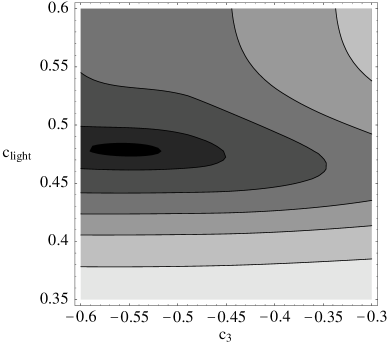
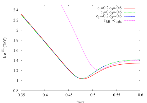
Figure 2: Lower bound on $\tilde{k}=k\,e^{-kL}$ as a function of $c_{3}$ and $c_{\mathrm{light}}$ for fixed $c_{1}=0.2$ and $c_{\rm RH}=-0.6$ (left panel). The different contours, from dark to light, correspond to $\tilde{k}=1030,1100,1300,1500,1700$ and $2000$ GeV, respectively. The minimum is $\tilde{k}_{\mathrm{min}}=1$ TeV, corresponding to $c_{3}\approx-0.55$ and $c_{\mathrm{light}}\approx 0.48$. In the right panel we show the lower bound on $\tilde{k}$ as a function of $c_{\mathrm{light}}$ for fixed $c_{RH}=c_{3}=-0.6$ and three values of $c_{1}$. We also show the lower bound on $\tilde{k}$ for $c_{1}=0.2$ and $c_{3}=-0.6$, assuming $c_{\rm RH}=-c_{\rm light}$. The mass of the first gauge KK modes is $m^{\rm gauge}_{1}\approx 2.5~{}\tilde{k}$.

The results are actually quite insensitive to the value of $c_{1}$, with slightly better results as we get $Q_{1}$ farther from the IR brane, i.e. larger $c_{1}$. If $Q_{1}$ is too far from the IR brane, however, it is not possible to generate the top quark mass, with a resulting upper bound $c_{1}\lesssim 0.3$. In Fig. 2 we show, in the left panel, the $2\sigma$ lower bound on $\tilde{k}$ as a function of $c_{3}$ and $c_{\mathrm{light}}$, for fixed $c_{1}=0.2$, whereas in the right panel we show the bound on $\tilde{k}$ as a function of $c_{\mathrm{light}}$ for fixed $c_{3}=-0.6$ and three different values of $c_{1}=-0.2,0,0.2$, displaying the mild dependence on this latter parameter. We also show in the same figure the effect of localizing the light RH quarks and leptons at the same point as the LH ones. The minimum of the fit then shifts to $-c_{\rm RH}=c_{\mathrm{light}}\approx 0.51$ with a lower bound $\tilde{k}\gtrsim 1.2$ TeV.

The dependence on the localization of the light fermions is easy to understand. The fit is virtually independent of the particular localization once the conformal point is crossed towards the UV brane, $c_{\mathrm{light}}\gtrsim 0.5$, due to the universal couplings of fermion zero modes to gauge boson KK modes in that case. There is of course a limit on how far from the IR brane we can get, given by the fact that we have to generate the fermion masses. For instance, the charm and strange masses force us to take the associated localization parameters below about 0.6. This is why we have taken $c_{\mathrm{light}}\leq 0.6$ in our plots. As we have emphasized, however, the results in that limit are independent of the particular localization of each light fermion, and we could take the first generation fermions to be farther away from the IR brane with similar results.

Also, as is clear from Fig. 2, bringing the light fermions very close to the IR brane does not improve the fit, due to the strong coupling to the gauge boson KK modes in that limit. However, the figure also shows a minimum when the light fermions are near the conformal point. It is well known that in this case the (light) fermions decouple from the KK excitations of the $W$ and $Z$ gauge bosons. It is nevertheless important to notice that they do not decouple from the KK excitations of the $SU(2)_{R}$ gauge bosons and, even near the conformal point, this leads to non-universal shifts in the gauge couplings of the SM fermions that cannot be neglected in the fit. To illustrate the relevance of such effects, if the custodial protection, $SU(2)_{V}\times P_{LR}$, is also implemented in the lepton sector, such non-universal shifts are enough to completely erase the dip in the $\chi^{2}$ near the conformal point. In that case, one finds a 2$\sigma$ lower bound of $\tilde{k}\gtrsim 1.4~{}\mathrm{TeV}$, obtained when the light fermions are near the UV brane (this is exactly as in Fig. 2, since in this region the $SU(2)_{R}$ gauge bosons quickly decouple from the low-energy physics), and the bound increases monotonically as the light fermions are brought closer to the IR brane. Such a feature is a direct result of the fermion couplings to the $SU(2)_{R}$ gauge bosons as specified by the embedding into bidoublets of $SU(2)_{L}\times SU(2)_{R}$. We explore other possibilities in section V.

Finally, the dependence on the last localization parameter, $c_{3}$, can also be easily understood. In the limit that the light fermions are near the IR brane ($c_{\mathrm{light}}\leq 0.5$), the loss of up-down universality as well as the strong coupling of light fermions to the gauge boson KK excitations dominate the fit, and therefore the details of the $b_{R}$ localization are irrelevant. This is the reason for the horizontal contours in the left panel of Fig. 2 for $c_{\mathrm{light}}\lesssim 0.5$. As the light fermions get farther from the IR brane, the $b$ asymmetries and branching fractions gain importance in the fit and therefore there is some dependence on the value of $c_{3}$. The fit shows that the EW precision observables select the region in which $b_{R}$ and the RH light fermions are localized close to the UV brane, whereas the LH light fermions are near the conformal point slightly towards the IR brane. In such a scheme the fermion mass hierarchies can be obtained from the RH fermion profiles. Note, however, that the light families, both LH and RH, could be localized close to the UV brane with only a slightly tighter bound on $\tilde{k}$.

V Effects of simple modifications

The result of the global fit gives an excellent idea of the typical bounds on the scale of new physics in this class of models. Nevertheless, they are indirect bounds and they should be interpreted accordingly.

In particular, contrary to the $T$ parameter and the $Zb_{L}\bar{b}_{L}$ coupling, that receive calculable corrections, the $S$ parameter can get arbitrary corrections from physics at the ultraviolet cut-off. This cut-off is warped down to the few TeV scale and therefore sizable contributions to the $S$ parameter cannot be ruled out. To estimate the effect such contribution might have, we have repeated the global fit with a contribution to the $S$ parameter that is twice as large as the one we have computed at one loop in our model. We have also re-done the fit with an arbitrary contribution to the $S$ parameter, that we have optimized for each value of the input parameters. The results of such fits are shown in Fig. 3 with solid line in the case of no extra contribution to the $S$ parameter beyond the one we have computed, dashed line for an extra contribution double the one we have computed in our model, and dotted line in the case that the extra contribution to the $S$ parameter has been optimized to minimize the $\chi^{2}$. The figure shows that a moderate extra positive contribution to the $S$ parameter worsens the fit slightly whereas optimizing the contribution leads to a considerably better fit, with a lower bound $\tilde{k}\gtrsim 650$ GeV (optimal $S$). Of course, this latter possibility is the result of a model tuned to optimize the fit, most likely requiring a fine-tuned UV completion, and therefore should not be taken as generic. Also, for such low values of $\tilde{k}$ the approximations we have made in linearizing the couplings to the Higgs in the present gauge-Higgs unification scenarios may have to be revisited. Nevertheless, this exercise gives us an idea of how changes in the model (or like in this case, effects of the UV completion of our model) can affect these bounds. In particular, a negative contribution to the $S$ parameter can be interesting Hirn:2006nt .

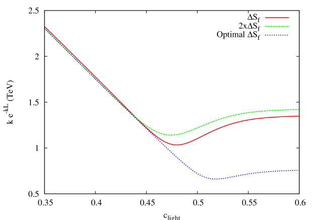
Figure 3: Lower bound on $\tilde{k}=k\,e^{-kL}$ as a function of $c_{\mathrm{light}}$ allowing different contributions to the $S$ parameter in the model of Section IV. The three lines correspond to the one-loop contribution from the spectrum in the model, Eq. (A.2) (solid line), twice that amount (dashed line) and a value of $\Delta S_{f}$ that minimizes the $\chi^{2}$ for each value of the parameters (dotted line). In all cases, $c_{1}=0.2$ and $c_{\rm RH}=c_{3}=-0.6$.

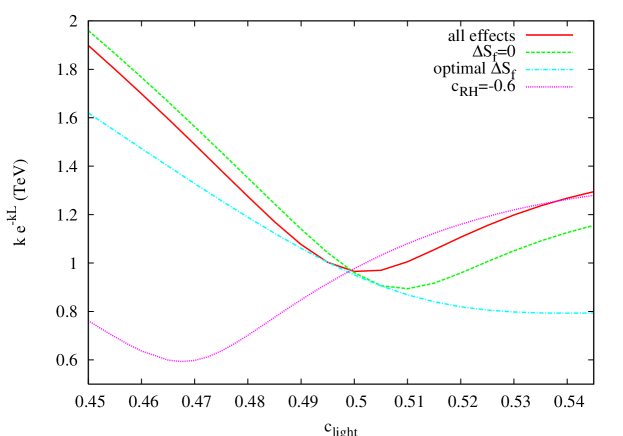
Figure 4: Lower bound on $\tilde{k}=k\,e^{-kL}$ as a function of $c_{\mathrm{light}}=-c_{\rm RH}$ when the light generations arise from doublets of $SU(2)_{L}$ or $SU(2)_{R}$, including all effects (solid line), setting the one-loop contributions to $\Delta S_{f}$ to zero (dashed line), and choosing values of $\Delta S_{f}$ that minimize the $\chi^{2}$ for each value of the parameters (dash-dotted line). We also show the lower bound on $\tilde{k}$ when the right-handed light fermions are localized at $c_{\rm RH}=-0.6$ (near the UV brane), as a function of the localization parameter for left-handed light fermions, $c_{\mathrm{light}}$ (dotted line). In all cases we have fixed $c_{1}=0.2$ and $c_{3}=-0.6$.

A second type of modification is obtained when the quarks of the first two families –as in the lepton sector– arise from doublets of $SU(2)_{L}$ or $SU(2)_{R}$, as opposed to bidoublets of $SU(2)_{L}\times SU(2)_{R}$. In this case, it might be difficult to generate the mixing between the first two quark generations and the third one. Nevertheless, we have repeated the global fit analysis in such a scenario, as shown in Fig. 4. When the LH and RH fermions have a common localization parameter, $c_{\rm light}=-c_{\rm RH}$, the fit exhibits a minimum corresponding to a $2\sigma$ bound of $\tilde{k}\approx 1~{}{\rm TeV}$, again around $c_{\rm light}\approx 0.5$. This corresponds to the conformal point, where the light generations decouple from the KK modes of the $SU(2)_{L}$ gauge bosons (solid line). Note, however, that this fit includes the fermion one-loop contributions to the $S$ parameter, $\Delta S_{f}$, that are sizable. If we do not include such loop contributions, the fit prefers that the light generations be localized somewhat closer to the UV brane (dashed line). This is contrary to the naive expectations, since when the presence of the $SU(2)_{R}$ gauge bosons is taken into account, the tree-level corrections to the couplings between the left-handed SM fermions and the gauge bosons vanish at a point slightly closer to the IR brane. The result we find can be explained by observing that, under the assumption $c_{\rm RH}=-c_{\rm light}$, we cannot simultaneously avoid the corrections to the couplings involving left- and right-handed fermions, and the global fit still prefers a region of parameter space where the couplings to the $SU(2)_{R}$ gauge bosons are somewhat suppressed (fermions closer to the UV brane). In fact, when the light RH quarks and leptons are localized near the UV brane, the fit shows a clear and pronounced minimum at $c_{\mathrm{light}}\approx 0.47$. In that case, one finds a lower bound on $\tilde{k}\gtrsim 600~{}{\rm GeV}$, due to an improvement in $A_{FB}^{b}$ resulting from a decrease in $A_{e}$. Finally, we have re-done the fit, again for $c_{RH}=-c_{\mathrm{light}}$, with an arbitrary contribution to the $S$ parameter, optimized to minimize the $\chi^{2}$ (dash-dotted line). As previously discussed, such a scenario could arise from a (possibly fine-tuned) UV completion.

We therefore conclude that both the calculable loop corrections, as well as various sources of nonuniversal shifts to the couplings between fermions and gauge bosons can place important restrictions, and that a global fit analysis is essential in a broad class of warped scenarios, whenever the light generations are not close to the UV brane. We find that the indirect bounds on $\tilde{k}$ are typically around a TeV.

VI Spectrum and phenomenological implications

We have seen that a global fit to EW precision observables allows KK excitations of the SM gauge bosons, together with $W_{R}^{\pm}$ and $Z^{\prime}$, as light as $m_{1}^{\mathrm{gauge}}\sim 2-3$ TeV over a wide region of parameter space in models with custodial protection of the $T$ parameter and the $Zb_{L}\bar{b}_{L}$ coupling. This opens up exciting possibilities for discovering these particles at the LHC and measuring their properties gaugeKK . In particular, the loop contribution to the $T$ parameter typically singles out a very specific localization of the third quark family ($t_{R}$ almost flat and $(t_{L},b_{L})$ near the IR brane), that leads to a distinct phenomenology.  The fermionic spectrum is even more exciting as it can be much lighter than the the spectrum of gauge boson KK modes. There are two reasons why KK fermions can be light in these models. One is the presence of large brane localized masses, and the other is the natural appearance of twisted boundary conditions, $(-,+)$ or $(+,-)$. Large brane localized masses, needed to generate the large top mass, are a generic feature of these models. In principle, one could get the top mass through brane localized masses that connect either bidoublets or singlets [see Eq. (11)]. However, in the case of localized masses connecting two bidoublets, the light KK bidoublet excitations will mix strongly with the top quark, inducing a negative $T$ parameter which is disfavored by the EW precision data. Thus, the top mass should be predominantly obtained by means of brane localized masses connecting singlets, and therefore light KK singlets are a generic prediction in these theories. On the other hand, light KK fermion bidoublets can arise from twisted boundary conditions, provided they do not mix strongly with the zero modes. In particular, our boundary conditions for $Q_{2}$, which ensure no mixing between the bidoublets $Q_{1}$ and $Q_{2}$, give quarks much lighter than $\tilde{k}$ provided that the $t_{R}$ wavefunction is nearly flat (i.e. $c_{2}\sim-0.5$), as required by the EW precision data.

$q^{\prime}$	Q	$\mbox{ }\quad m_{q^{\prime}}$ (GeV)	decay
$q_{1}^{1}$	$\frac{2}{3}$	$\sim 200-500$	$q_{1}^{1}\to Zu,\quad(100\%)$
$q_{1}^{2}$	$\frac{2}{3}$	$\sim 200-500$	$q_{1}^{2}\to Zc,\quad(100\%)$
$q_{2}^{1}$	$\frac{2}{3}$	$\sim 200-500$	$q_{2}^{1}\to Hu,\quad(100\%)$
$q_{2}^{2}$	$\frac{2}{3}$	$\sim 200-500$	$q_{2}^{2}\to Hc,\quad(100\%)$
$\chi_{2}^{u_{1}}$	$\frac{5}{3}$	$\sim 200-500$	$\chi_{2}^{u_{1}}\to Wu,\quad(100\%)$
$\chi_{2}^{u_{2}}$	$\frac{5}{3}$	$\sim 200-500$	$\mbox{ }\quad\chi_{2}^{u_{2}}\to Wc,\quad(100\%)\mbox{ }\quad$
$q^{\prime d_{1}}$	$-\frac{1}{3}$	$\sim 200-500$	$q^{\prime d_{1}}\to Wu,\quad(100\%)$
$q^{\prime d_{2}}$	$-\frac{1}{3}$	$\sim 200-500$	$q^{\prime d_{2}}\to Wc,\quad(100\%)$

Table 1: Electric charges, typical masses and decay channels for the KK excitations of the first two quark families with masses below 1 TeV. Here, $q^{i}_{1}$ and $q^{i}_{2}$ are linear combinations of the gauge eigenstates $q^{\prime u_{i}}$ and $\chi^{d_{i}}_{2}$ of Eq. (10).

The typical fermionic spectrum in our model is shown in Tables 1 and 2. For each of the first two families, the four quarks in $Q_{2}$ of Eq. (10) have very light KK excitations for $c_{\mathrm{RH}}\lesssim-0.5$ DelAguila:2001pu ; Agashe:2004bm . As shown in Table 1, there are eight quarks with almost degenerate masses of a few hundred GeV. Four of them have charge $2/3$, and two decay almost exclusively to $Z+j$ (where $j$ denotes a jet from an up or charm quark) while the other two decay to $H+j$. There are also two light quarks with charge $-1/3$ and two with exotic charge $5/3$, which decay to $W+j$.

For the third family, we have three essentially degenerate KK excitations with charges $5/3$, $2/3$ and $-1/3$. There is a fourth KK excitation with charge $+2/3$ and a mass very close to the previous states. In Fig. 5 (left), we show the variation of the masses of the three lightest, degenerate KK quark excitations –that couple strongly to the third generation– as functions of the basic parameters of the model, for fixed $c_{1}=0.2$ and $\tilde{k}$ saturating the lower bound from the global fit that assumes a common localization parameter for all the light fermions (both LH and RH chiralities). Fig. 5 (right) shows the masses of the three lightest KK modes with charge $2/3$ as a function of $c_{\mathrm{light}}$ for fixed values of $c_{1}=0.2$ and $c_{3}=-0.6$. As seen in the figures, quarks as light as about $400$ GeV are allowed in the region in which the light fermions are near the conformal point and $b_{R}$ is near the UV brane.

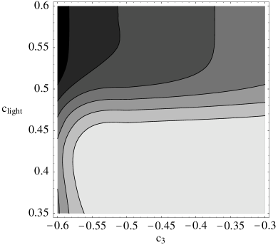
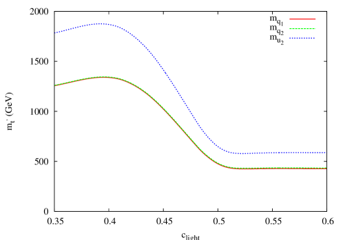
Figure 5: Mass of the first level quarks of the third generation for the model of Section IV and a $\tilde{k}$ that saturates the bound, assuming $c_{\rm RH}=-c_{\rm light}$ (dotted curve in the right panel of Fig. 2). In the left panel we show the masses of the three degenerate quarks with charges $5/3$, $2/3$ and $-1/3$ as a function of $c_{3}$ and $c_{\mathrm{light}}$, for fixed $c_{1}=0.2$. The different contours, from dark to light, correspond to $m_{1}=500,600,750,1000,1250$ and $1500$ GeV, respectively. In the right panel we show the mass of the three lightest quark KK modes with charge 2/3 as a function of $c_{\mathrm{light}}$ for fixed $c_{1}=0.2$ and $c_{3}=-0.6$.

As an example, we show in Table 2 the typical values for the light KK excitations for the third family when $c_{\mathrm{light}}=-c_{\rm RH}=0.52$, $c_{1}=0.2$, $c_{2}=-0.49$, $c_{3}=-0.6$, $\tilde{k}=1.2$ TeV, and localized mass parameters such that the SM quark masses and CKM matrix are correctly reproduced. There are three quarks with charge $2/3$, two of them with almost degenerate masses of about $370$ GeV and the third one with mass of about $500$ GeV. All of them have decays to $Z+t$, $H+t$ and $W+b$ as shown in the table. There are also two other light KK modes, one with charge $-1/3$ and another with exotic charge $5/3$, with degenerate masses of order $370$ GeV and which decay almost exclusively to $W+t$. Note that there is a small but non-negligible probability for the heavier of the three quarks with charge $2/3$ to decay into the quarks of mass $\sim 370$ GeV (with either charge).

$q^{\prime}$	Q	$m_{q^{\prime}}$ (GeV)	decay
$q_{1}$	$\frac{2}{3}$	369	$\begin{array}[]{l}q_{1}\to Zt,\quad(20\%)\\ q_{1}\to Ht,\quad(60\%)\\ q_{1}\to Wb,\quad(20\%)\end{array}$
$q_{2}$	$\frac{2}{3}$	373	$\begin{array}[]{l}q_{2}\to Zt,\quad(9\%)\\ q_{2}\to Ht,\quad(70\%)\\ q_{2}\to Wb,\quad(21\%)\end{array}$
$u_{2}$	$\frac{2}{3}$	504	$\begin{array}[]{l}u_{2}\to Zt,\quad(13\%)\\ u_{2}\to Ht,\quad(40\%)\\ u_{2}\to Wb,\quad(41\%)\\ u_{2}\to Zq_{1},\quad(1.5\%)\\ u_{2}\to Wq^{\prime d_{3}},\quad(2.5\%)\\ u_{2}\to W\chi^{u_{3}}_{2},\quad(2.\%)\end{array}$
$\chi_{2}^{u_{3}}$	$\frac{5}{3}$	369	$\chi_{2}^{u_{3}}\to Wt,\quad(100\%)$
$q^{\prime d_{3}}$	$-\frac{1}{3}$	369	$q_{2}^{\prime d_{3}}\to Wt,\quad(100\%)$

Table 2: Electric charges and typical masses and decay channels for the KK excitations of the third quark family with masses below 1 TeV. We have fixed $c_{\rm light}=-c_{\rm RH}=0.52$, $c_{1}=0.2$, $c_{2}=-0.49$, $c_{3}=-0.6$ and $\tilde{k}=1.2$ TeV. Here, $q_{1}$, $q_{2}$ and $u_{2}$ are mainly admixtures of the gauge eigenstates $q^{\prime u_{3}}$, $\chi^{d_{3}}_{2}$ and $u^{\prime 3}$ of Eq. (10).

The rest of the fermion KK modes have masses typically above $1$ TeV. In the following we shall discuss the potential for searches for the first level of fermionic excitations at the Tevatron and the LHC. These models can also have very interesting collider implications in B and top physics Agashe:2006wa ; Aquino:2006vp but we postpone their study for future work.

VI.1 Fermion KK modes at the Tevatron

The Tevatron has excellent capabilities to search for the light KK excitations of the first two generation quarks shown in Table 1. In particular, there are ongoing Tevatron searches for heavy quarks decaying to $W+j$ Wj:note and $Z+j$ Zj:note , which apply directly to our model. The first analysis examines the $W+j$ mass spectrum and compares to the distribution expected from a generic forth-generation top quark. The $Z+j$ analysis does not assume any specific model, but rather looks at the tail of the jet energy distribution for an excess above the SM expectation. A similar analysis looks at the $p_{T}$ distribution of the $Z$ boson, and in principle could also be sensitive to signals from our model. Using the results of these analyses and taking into account the enhancement factor in the production cross section due to the multiplicity of quarks (4 in the $W+j$ analysis and 2 in the $Z+j$ one), we obtain the following lower bound on the mass of the light KK excitations

$$m_{q}\geq\left\{\begin{array}[]{ll}325~{}(410)\mbox{ GeV},&W+j\mbox{ with }0.76~{}(\mbox{projected}~{}8)~{}\mathrm{fb}^{-1}~{},\\ 300\mbox{ GeV},&Z+j~{}.\end{array}\right.$$ (33)

Figure 6 shows the bound on $\tilde{k}$ from the fit to EW precision data together with the constraints on our parameter space that result from these direct searches at the Tevatron. The direct search analysis eliminates the region of parameter space in which the light fermions are localized towards the UV brane. When combined with the EW precision analysis, they slightly strengthen the lower bound on $\tilde{k}$.

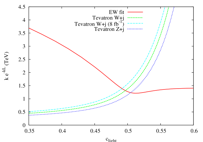
Figure 6: Lower bound on $\tilde{k}=k\,e^{-kL}$ as a function of $c_{\mathrm{light}}=-c_{\rm RH}$ for fixed $c_{1}=0.2$ and $c_{3}=-0.6$. The different lines correspond to the bounds from EW precision observables (solid), the $W+$ jets analysis at Tevatron with $0.76~{}\mathrm{fb}^{-1}$ (dashed), the projected exclusion reach to $8~{}\mathrm{fb}^{-1}$ in that same channel (dotted-dashed) and $Z+$ jets analysis at Tevatron (dotted). The regions below the curves are excluded.

Final states with $Z$ bosons could also lead to a signature with missing energy and jets. Searches for squarks and gluinos might be sensitive to a signal of this type. It is difficult to relate the experimental results to our model without performing detailed simulations. However, this channel might become interesting with a sufficiently large integrated luminosity.

We have considered other searches at the Tevatron, such as the tri-lepton, same-sign di-lepton, and four-lepton searches. However, these are usually rather model-dependent and apply cuts which tend to eliminate our signal. In particular, leptons reconstructing the $Z$ mass peak as well as jets are typically disallowed.

A very interesting feature is the presence of two light quarks that decay exclusively into $H+j$. If these quarks have masses around $300$ GeV, their production cross section will be of the same order of magnitude as Higgs production through gluon fusion for a light Higgs. As there are two such quarks, and two Higgs bosons in every event, there will be a sizable enhancement to the inclusive Higgs signal. It should be noted, however, that some sources of background (such as $WW+$ jets or $ZZ+$ jets) are also enhanced due to the decays of other light KK excitations, and a careful analysis of signal and background is necessary to assess Tevatron prospects for Higgs discovery in this model.

Finally, the KK excitations of the third quark generation, as shown in Table 2, are on the verge of the projected sensitivity for the Tevatron.

VI.2 Fermion KK modes at the LHC

The prospects for discovery of the light KK quark excitations of the first two families are more promising at the LHC. In principle, similar techniques as those used at the Tevatron could lead directly to a discovery, although the increase in production comes at the cost of a larger background from di-boson and top-quark production.

Quarks decaying to $H+j$ enhances Higgs production at the LHC with respect to the Standard Model. This cross-section is of the same order as Higgs gluon fusion production, provided the quarks are not much heavier than about $400$ GeV. If the Higgs is heavy enough to decay to $ZZ$ we have the following enhanced contribution to the inclusive $H\to ZZ$ cross section,

$$\sigma(H\to ZZ)_{\mathrm{incl}}\approx 2\sigma(q^{\prime}\bar{q}^{\prime})B[2-B]+\sigma(gg\to H)B~{},$$ (34)

where we have included the multiplicity of the KK fermions, and where $B\equiv{\rm BR}(H\to ZZ)\sim 0.02-0.25$ for $m_{H}\sim 120-200$ GeV Carena:2002es . For these values of $B$, there can easily be an enhancement in the inclusive $H\rightarrow ZZ$ of order a few. Note that there is also a contribution to the background from quarks decaying to $Z+j$ although the mass reconstruction in this channel seems precise enough to efficiently cut that background. Another clean channel would be $H\to\gamma\gamma$ for which we can take advantage of the enhancement of Higgs production without suffering a larger background from the decays of the lighter KK modes. Note that the loop-induced couplings, such as $gg\rightarrow H$ and $H\rightarrow\gamma\gamma$, are not significantly modified by the extra quark states. The reason is that these heavy quark states receive only a very small contribution to their masses from EW symmetry breaking, and as a result their effective (diagonal) Yukawa couplings are very suppressed.

There is an important distinction to be made between the first two generations and the third one. While the Tevatron is able to probe masses on the order of $300$ GeV or higher, these constraints can be evaded for the first two generations. If we switch the boundary conditions of the multiplet $Q_{2}$ for the first two families, the excitations of the first two quark generations become heavier, without affecting the EW fit. In that case the zero modes for the first two generations can be localized near the UV brane and the nice features of the mass generation through wavefunction suppressions preserved, as well as the flavor universality of the corrections (which become independent of the particular localization parameter in this limit). Nonetheless, the KK quark excitations of the third quark generation remain light, and well within the reach of the LHC Aguilar-Saavedra:2005pv ; T:littleHiggs (and possibly of the Tevatron).

Also for the third generation, the degenerate doublets with different hypercharges and large mixings with singlets give additional Higgs production channels which will greatly enhance the signals in inclusive Higgs searches and searches in the $ttH$ channel. The Higgs discovery reach will be even better than the one found in previous studies Aguilar-Saavedra:2006gw , which considered singlets, due to the enhanced decay ratio to Higgs ($\sim 40-70\%$ vs $25\%$ for singlets).

One will notice that nearly all of the final states listed in Table 2 result in top quarks in the final state. This suggests that inclusive top searches would be useful for finding these particles at the LHC. Another interesting signature might be multiple jets, some of them with $b$-quarks, and possibly high-$p_{T}$ leptons or missing energy.

Finally, the exotic quantum numbers of the fermion KK excitations of the third generation can give rise to spectacular new signatures. For instance, the quarks with electric charges $5/3$ and $-1/3$ have similar decay channels with four $W$’s

$$q^{\prime}\bar{q}^{\prime}\to W^{+}W^{-}t\bar{t}\to W^{+}W^{+}W^{-}W^{-}b\bar{b}~{}.$$ (35)

This can lead to a very clean final state $e^{+}e^{+}\mu^{-}\mu^{-}+b\bar{b}+\not\!\!E_{T}$ with very little background. Furthermore, for the charge $5/3$, we have two $W$’s of the same charge belonging to the same decay chain, which could be identified by a pair of same-sign leptons. Also, as seen in Table 2, $u_{2}$ has a non-negligible branching fraction into the lighter charge $2/3$ states, which can lead to a spectacular signal with a $6Wb\bar{b}$ final state.

VII Conclusions

Models with warped extra dimensions explain in a compelling way the hierarchy between the Planck and EW scales. Bulk fermions provide also a rationale for the observed hierarchy of fermion masses and the absence, for the light fermions, of large flavor changing neutral currents or large new effects from physics above the ultraviolet cut-off of the theory. The SM gauge bosons and third generation quarks, however, have a sizable coupling to heavy states through the Higgs field. These couplings induce large corrections to the $T$ parameter and the coupling of the left-handed bottom quark to the $Z$ gauge boson unless some symmetry forbids them. An enlarged bulk gauge symmetry can act as a custodial symmetry, $SU(2)_{V}\times P_{LR}$, that protects both the $T$ parameter and the $Zb_{L}\bar{b}_{L}$ coupling. When such a symmetry is broken only on the UV brane, these two observables acquire a distinctive status: they are insensitive to UV physics except for effects that are suppressed by a scale of order $M_{\mathrm{Pl}}$. This means that, for all practical purposes, they are calculable. We find that typically the one-loop corrections to these observables are sufficiently important that they need to be included when analyzing the bounds on these models. Furthermore, for the fermion quantum numbers required to obtain the SM fermions while preserving the custodial symmetry, these loop corrections are correlated. Thus, they are a generic feature of models with warped extra dimensions and custodial symmetry $SU(2)_{V}\times P_{LR}$, no matter whether the Higgs is a fundamental scalar, the extra dimensional component of a gauge field (gauge-Higgs unification) or not present (Higgsless models). The precise values of the $T$ parameter and the $Zb_{L}\bar{b}_{L}$ coupling are model-dependent, but we have identified the contributions that are generically present under the assumption of a custodial symmetry.

We have illustrated these features in a particular model of gauge-Higgs unification. We have computed all the relevant tree-level effects on EW precision observables plus the leading one-loop corrections to the $T$ parameter and the $Zb_{L}\bar{b}_{L}$ coupling. By performing a global fit to all relevant EW precision observables we have obtained a lower bound on the masses of the gauge boson KK excitations of about 2.5 TeV. This bound is saturated when the left-handed light fermions have nearly flat wavefunctions (the conformal point), while the right-handed light fermions are localized near the UV brane. However, very similar bounds are found in a large region of parameter space in which all the light fermions are localized far from the IR brane. In the latter case, the fit is dominated by a universal shift of the fermion coupling to the SM gauge bosons that can be redefined into a pure oblique correction to the $S$ parameter, although the correlation between the $T$ parameter and the $Zb_{L}\bar{b}_{L}$ coupling also have a noticeable effect. Contrary to these two latter observables, the $S$ parameter is not protected by any symmetry and can receive corrections from physics above the UV cut-off. Assuming an optimal correction to the $S$ parameter from UV physics, such that the $\chi^{2}$ of the fit is minimized with respect to $S$ for each point in parameter space, we have obtained a lower bound on the mass of the gauge boson KK modes of $\sim 1.6$ TeV, which is completely dominated by the observables in the $b$ sector and is therefore difficult to evade (as those observables are dominated by the $Zb_{L}\bar{b}_{L}$ coupling that is calculable in these models).

Regarding the fermionic spectrum, there can be a wealth of new vector-like quarks with exotic quantum numbers and masses as low as a few hundred GeV. These modes can be light enough for the Tevatron to have started probing part of the parameter space. We have discussed the bounds that current Tevatron analyses place on our model. Interestingly enough, some of these modes have exotic decay channels, for instance some of them decaying essentially $100\%$ into $H$ plus jets. This opens up interesting prospects for Higgs physics both at the Tevatron and the LHC. Heavy quarks decaying to $W+j$ or $Z+j$ have been searched for at the Tevatron, with current limits of about $325$ GeV and $300$ GeV, respectively, for the quark multiplicities present in our model. Excitations of the third generation quarks can have masses of order $400$ GeV that might be within reach of the Tevatron. They typically decay to third generation quarks with non-standard branching ratios, naturally enhancing Higgs production. Decays to top quarks through gauge bosons induce a very interesting decay chain with four gauge bosons ($4W$ or $2W+2Z$) and two $b$’s, as well as a possible final state with six $W$’s and two $b$’s, that would give a spectacular signal at the LHC. In particular, heavy quarks (with typical masses of order $500$ GeV) with electric charge $5/3$ produce two same sign $W$ in each decay chain whereas those with charge $-1/3$ will give one $W$ of each sign per chain. The process

$$pp\to q_{5/3,-1/3}\bar{q}_{5/3,-1/3}\to W^{+}tW^{-}\bar{t}\to W^{+}W^{+}bW^{-}W^{-}\bar{b}\to\mu^{+}\mu^{+}e^{-}e^{-}b\bar{b}\not\!\!E_{T},$$ (36)

would lead to an easy discovery of these modes with almost no background.

Note added: During the final stages of this article, we received references Cacciapaglia:2006mz and Contino:2006qr , which partially overlap with ours in the study of different aspects of models with warped extra dimensions and custodial protection of the $Zb_{L}\bar{b}_{L}$ coupling. However they do not discuss the importance of the calculable one-loop corrections to the $T$ parameter or the $Zb_{L}\bar{b}_{L}$ coupling, nor perform a detailed global fit to the EW precision observables.

*

Appendix A 4D Effective theory

In this appendix we give the details of the matching between the 5D theory and the 4D theory used to perform the global fit analysis. We compute the dimension-6 operators and put them in the form of Eq. (12).

A.1 Integration of heavy gauge bosons

We can perform the tree-level integration of heavy gauge bosons in an $SU(2)_{L}\times U(1)_{Y}$ gauge invariant way by splitting the full covariant derivative into a Standard Model part and a part involving heavy physics,

$$D_{\mu}^{\mathrm{full}}=D_{\mu}-\mathrm{i}\Big{[}g_{5\,L}\tilde{W}^{a}_{L\mu}T^{a}_{L}+g_{5\,R}\tilde{W}^{b}_{R\mu}T^{b}_{R}+g_{5}^{\prime}Y\tilde{B}_{\mu}+g_{5\,Z^{\prime}}Q_{Z^{\prime}}\tilde{Z}^{\prime}_{\mu}\Big{]}~{},$$ (37)

where $D_{\mu}$ represents the SM covariant derivative and we use tildes to denote the massive KK components of the 5D fields. In the above, $a=1,2,3$ label the $SU(2)_{L}$ gauge bosons, $b=1,2$ label the charged $SU(2)_{R}$ gauge bosons, and $B_{\mu}$ and $Z^{\prime}_{\mu}$ are the following two combinations of neutral gauge bosons

$$B_{\mu}=\frac{g_{5\,X}W^{3}_{R\,\mu}+g_{5\,R}X_{\mu}}{\sqrt{g^{2}_{5\,R}+g^{2}_{5\,X}}}~{},\quad\quad\quad Z^{\prime}_{\mu}=\frac{g_{5\,R}W^{3}_{R\,\mu}-g_{5\,X}X_{\mu}}{\sqrt{g^{2}_{5\,R}+g^{2}_{5\,X}}}~{},$$ (38)

with $g_{5\,R},g_{5\,X}$ the five-dimensional coupling constants of the $SU(2)_{R}$ and $U(1)_{X}$ groups, respectively, while the hypercharge and $Z^{\prime}$ gauge couplings are

$$g_{5}^{\prime}=\frac{g_{5\,R}\,g_{5\,X}}{\sqrt{g^{2}_{5\,R}+g^{2}_{5\,X}}}~{},\quad\quad\quad g_{5\,Z^{\prime}}=\sqrt{g^{2}_{5\,R}+g^{2}_{5\,X}}~{}.$$ (39)

The charges are

$$\frac{Y}{2}=T^{3}_{R}+Q_{X}~{},\quad\quad\quad Q_{Z^{\prime}}=\frac{g_{5\,R}^{2}T^{3}_{R}-g_{5\,X}^{2}Q_{X}}{g_{5\,R}^{2}+g_{5\,X}^{2}}~{},$$ (40)

so that the electric charge is

$$Q=T^{3}_{L}+T^{3}_{R}+Q_{X}~{}.$$ (41)

The Lagrangian involving heavy fields then reads (terms with two heavy fields except for kinetic terms give higher order corrections and are therefore not written)

$$\Delta\mathcal{L} = \frac{1}{2}\tilde{W}^{a}_{L\mu}\mathcal{O}^{\mu\nu}\tilde{W}^{a}_{L\nu}+\frac{1}{2}\tilde{W}^{b}_{R\mu}\mathcal{O}^{\mu\nu}\tilde{W}^{b}_{R\nu}+\frac{1}{2}\tilde{B}_{\mu}\mathcal{O}^{\mu\nu}\tilde{B}_{\nu}+\frac{1}{2}\tilde{Z}^{\prime}_{\mu}\mathcal{O}^{\mu\nu}\tilde{Z}^{\prime}_{\nu}$$ (42)

$$+ g_{5\,L}\tilde{J}^{a\mu}_{L}\tilde{W}^{a}_{L\mu}+g_{5\,R}\tilde{J}^{b\mu}_{R}\tilde{W}^{b}_{R\mu}+g^{\prime}_{5}\tilde{J}^{\mu}_{Y}\tilde{B}_{\mu}+g_{5\,Z^{\prime}}\tilde{J}^{\mu}_{Z^{\prime}}\tilde{Z}^{\prime}_{\mu}~{},$$

where

$${\cal{O}}^{\mu\nu}\equiv\left[\eta^{\mu\nu}\partial^{2}-\partial^{\mu}\partial^{\nu}+\eta^{\mu\nu}\partial_{y}\left(e^{-2ky}\partial_{y}\right)\right]~{},$$ (43)

and the effective currents read

$$\tilde{J}^{a\mu}_{L} = e^{-2\sigma}[(T^{a}_{L}h)^{\dagger}\mathrm{i}D^{\mu}h+\mathrm{h.c.}]+e^{-3\sigma}\bar{\psi}\gamma^{\mu}T^{a}_{L}\psi~{},$$ (44)

$$\tilde{J}^{b\mu}_{R} = e^{-2\sigma}[(T^{b}_{R}h)^{\dagger}\mathrm{i}D^{\mu}h+\mathrm{h.c.}]+e^{-3\sigma}\bar{\psi}\gamma^{\mu}T^{b}_{R}\psi~{},$$ (45)

$$\tilde{J}^{\mu}_{Y} = e^{-2\sigma}[(Yh)^{\dagger}\mathrm{i}D^{\mu}h+\mathrm{h.c.}]+e^{-3\sigma}\bar{\psi}\gamma^{\mu}Y\psi~{},$$ (46)

$$\tilde{J}^{\mu}_{Z^{\prime}} = e^{-2\sigma}[(Q_{Z^{\prime}}h)^{\dagger}\mathrm{i}D^{\mu}h+\mathrm{h.c.}]+e^{-3\sigma}\bar{\psi}\gamma^{\mu}Q_{Z^{\prime}}\psi~{}.$$ (47)

The equations of motion for the heavy fields can now be easily written and solved. For instance, for $\tilde{W}^{a}_{L}$, the equations of motion are

$$\mathcal{O}^{\mu\nu}\tilde{W}^{a}_{L\nu}=-g_{5\,L}\tilde{J}^{a\mu}_{L}~{},$$ (48)

with solution

$$\tilde{W}^{a}_{L\mu}(p;y)=g_{5\,L}\int_{0}^{L}\mathrm{d}y^{\prime}\,\widetilde{G}^{(++)}_{\mu\nu}(p;y,y^{\prime})\tilde{J}^{a\nu}_{L}(p;y^{\prime})~{},$$ (49)

where $\widetilde{G}^{(++)}_{\mu\nu}$ is the propagator for the KK modes obeying $(+,+)$ boundary conditions (the inverse of the differential operator in Eq. (48) with the zero-mode subtracted), and $p$ is the 4-dimensional momentum. Inserting the solution for all the heavy modes back into the Lagrangian we obtain the following dimension six effective Lagrangian

$$\Delta\mathcal{L}_{6} = \frac{1}{2}\int_{0}^{L}\mathrm{d}y\mathrm{d}y^{\prime}\,\Big{[}g^{2}_{5\,_{L}}\tilde{J}^{a\mu}_{L}\widetilde{G}^{(++)}_{\mu\nu}\tilde{J}^{a\nu}_{L}+g^{\prime\,2}_{5}\tilde{J}^{\mu}_{Y}\widetilde{G}^{(++)}_{\mu\nu}\tilde{J}^{\nu}_{Y}$$ (50)

$$\phantom{\frac{1}{2}\int_{0}^{L}\mathrm{d}y\mathrm{d}y^{\prime}}+g^{2}_{5\,_{R}}\tilde{J}^{b\mu}_{R}\widetilde{G}^{(-+)}_{\mu\nu}\tilde{J}^{b\nu}_{R}+g^{2}_{5\,Z^{\prime}}\tilde{J}^{\mu}_{Z^{\prime}}\widetilde{G}^{(-+)}_{\mu\nu}\tilde{J}^{\nu}_{Z^{\prime}}\Big{]}~{}.$$

Note that these are already operators of dimension six. Thus, the propagators have to be evaluated at zero momentum. The relevant expression is

$$\widetilde{G}_{\mu\nu}(p=0,y,y^{\prime})=\eta_{\mu\nu}\widetilde{G}_{p=0}(y,y^{\prime})+\mathcal{O}(p^{2}),$$ (51)

where for $(+,+)$ boundary conditions,

$$\widetilde{G}^{(++)}_{p=0}(y,y^{\prime}) = \frac{1}{4k(kL)}\bigg{\{}\frac{1-e^{2kL}}{kL}+e^{2ky_{<}}(1-2ky_{<})+e^{2ky_{>}}\left[1+2k(L-y_{>})\right]\bigg{\}}~{},$$ (52)

while for $(-,+)$ boundary conditions

$$\widetilde{G}^{(-+)}_{p=0}(y,y^{\prime}) = -\frac{1}{2k}\left[e^{2ky_{<}}-1\right]~{}.$$ (53)

Here $y_{<}$ ($y_{>}$) denote the smallest (largest) of $y$ and $y^{\prime}$, the fifth-dimensional coordinate.

The full $y$ dependence of the effective Lagrangian can be encoded in the following coefficients,

$$\delta_{++}^{2} = \frac{L}{2}\int_{0}^{L}\mathrm{d}y\mathrm{d}y^{\prime}\,e^{-2ky}f_{H}^{2}(y)\widetilde{G}^{(++)}_{0}(y,y^{\prime})e^{-2ky^{\prime}}f_{H}^{2}(y^{\prime}),$$ (54)

$$G^{++}_{\psi} = \frac{1}{2}\int_{0}^{L}\mathrm{d}y\mathrm{d}y^{\prime}\,|f_{\psi}(y)|^{2}\widetilde{G}^{(++)}_{0}(y,y^{\prime})e^{-2ky^{\prime}}f_{H}^{2}(y^{\prime}),$$ (55)

$$G^{++}_{\psi\tilde{\psi}} = \frac{1}{L}\int_{0}^{L}\mathrm{d}y\mathrm{d}y^{\prime}\,|f_{\psi}(y)|^{2}\widetilde{G}^{(++)}_{0}(y,y^{\prime})|f_{\tilde{\psi}}(y^{\prime})|^{2},$$ (56)

with similar definitions for $\delta_{-+}^{2}$, $G^{-+}_{\psi}$ and $G^{-+}_{\psi\tilde{\psi}}$ in terms of the propagator of Eq. (53). We have used the $y$-dependence of the fermion and Higgs zero modes

$$\psi(x,y) = \frac{e^{3\sigma/2}}{\sqrt{L}}f_{\psi}(y)\psi(x)+\ldots,$$ (57)

$$h(x,y) = f_{H}(y)h(x)+\ldots~{},$$ (58)

with the Higgs field, $h(x)$, written here as a doublet of $SU(2)_{L}$. Technically, the fermionic dependence is more complicated due to the non-trivial mass mixing on the brane. The analysis of Ref. Han:2004az , however, assumes flavor universality for the first two families and that will actually be a very good approximation for the range of parameters we will consider in the global fit (otherwise large flavor violation involving the first two families would be generated, in gross conflict with experimental data).

Note that, even after evaluation of the propagators at zero momentum and integration over the extra dimension, the effective Lagrangian in Eq.(50) is not yet in the basis of Buchmuller:1985jz . Simple manipulations of the operators involving integration by parts and use of the completeness of the Pauli matrices takes us to the desired basis. The resulting effective Lagrangian then reads,

$$\Delta\mathcal{L}_{6} = \alpha_{h}\mathcal{O}_{h}+\alpha^{t}_{hl}\mathcal{O}^{t}_{hl}+\alpha^{t}_{hq}\mathcal{O}^{t}_{hq}+\alpha^{s}_{hl}\mathcal{O}^{s}_{hl}+\alpha^{s}_{hq}\mathcal{O}^{s}_{hq}+\alpha_{hu}\mathcal{O}_{hu}+\alpha_{hd}\mathcal{O}_{hd}+\alpha_{he}\mathcal{O}_{he}$$ (59)

$$+ \alpha^{t}_{ll}\mathcal{O}^{t}_{ll}+\alpha^{t}_{lq}\mathcal{O}^{t}_{lq}+\alpha^{s}_{ll}\mathcal{O}^{s}_{ll}+\alpha^{s}_{lq}\mathcal{O}^{s}_{lq}+\alpha_{le}\mathcal{O}_{le}+\alpha_{qe}\mathcal{O}_{qe}+\alpha_{lu}\mathcal{O}_{lu}+\alpha_{ld}\mathcal{O}_{ld}$$

$$+ \alpha_{ee}\mathcal{O}_{ee}+\alpha_{eu}\mathcal{O}_{eu}+\alpha_{ed}\mathcal{O}_{ed}+\ldots~{},$$

where the list of operators was given in Eqs. (13)-(25), and the different coefficients have the following expressions:

$$\begin{array}[]{cclcccl}\alpha_{h}&=&g^{\prime\,2}[\delta^{2}_{++}-\delta^{2}_{-+}]~{},\\ \alpha^{t}_{hl}&=&\frac{g_{L}^{2}}{2}G_{l}^{++},&&\alpha^{t}_{hq}&=&\frac{g_{L}^{2}}{2}G_{q}^{++}~{},\\ \alpha^{s}_{hl}&=&-\frac{g^{\prime\,2}}{2}G^{++}_{l}+g_{R}^{2}Q_{Z^{\prime}}(l)G^{-+}_{l}~{},&&\alpha^{s}_{hq}&=&\frac{g^{\prime\,2}}{6}G^{++}_{q}+g_{R}^{2}Q_{Z^{\prime}}(q)G^{-+}_{q}~{},\\ \alpha_{hu}&=&\frac{2g^{\prime\,2}}{3}G^{++}_{u}+g_{R}^{2}Q_{Z^{\prime}}(u)G^{-+}_{u}~{},&&\alpha_{hd}&=&-\frac{g^{\prime\,2}}{3}G^{++}_{d}+g_{R}^{2}Q_{Z^{\prime}}(d)G^{-+}_{d}~{},\\ \alpha_{he}&=&-g^{\prime\,2}G^{++}_{e}+g_{R}^{2}Q_{Z^{\prime}}(e)G^{-+}_{e}~{},\\ \alpha^{t}_{ll}&=&g_{L}^{2}G_{ll}^{++}~{},&&\alpha^{t}_{lq}&=&g_{L}^{2}G_{lq}^{++}~{},\\ \alpha^{s}_{ll}&=&\frac{g^{\prime\,2}}{4}G_{ll}^{++}+g^{2}_{Z^{\prime}}Q_{Z^{\prime}}^{2}(l)G_{ll}^{-+}~{},&&\alpha^{s}_{lq}&=&-\frac{g^{\prime\,2}}{12}G_{lq}^{++}+g^{2}_{Z^{\prime}}Q_{Z^{\prime}}(l)Q_{Z^{\prime}}(q)G_{lq}^{-+}~{},\\ \alpha_{le}&=&\frac{g^{\prime\,2}}{2}G_{le}^{++}+g^{2}_{Z^{\prime}}Q_{Z^{\prime}}(l)Q_{Z^{\prime}}(e)G_{le}^{-+}~{},&&\alpha_{qe}&=&-\frac{g^{\prime\,2}}{6}G_{qe}^{++}+g^{2}_{Z^{\prime}}Q_{Z^{\prime}}(q)Q_{Z^{\prime}}(e)G_{qe}^{-+}~{},\\ \alpha_{lu}&=&-\frac{g^{\prime\,2}}{3}G_{lu}^{++}+g^{2}_{Z^{\prime}}Q_{Z^{\prime}}(l)Q_{Z^{\prime}}(u)G_{lu}^{-+}~{},&&\alpha_{ld}&=&\frac{g^{\prime\,2}}{6}G_{ld}^{++}+g^{2}_{Z^{\prime}}Q_{Z^{\prime}}(l)Q_{Z^{\prime}}(d)G_{ld}^{-+}~{},\\ \alpha_{ee}&=&g^{\prime\,2}G_{ee}^{++}+g^{2}_{Z^{\prime}}Q_{Z^{\prime}}(e)^{2}G_{ee}^{-+}~{},&&\alpha_{eu}&=&-\frac{2g^{\prime\,2}}{3}G_{eu}^{++}+g^{2}_{Z^{\prime}}Q_{Z^{\prime}}(e)Q_{Z^{\prime}}(u)G_{eu}^{-+}~{},\\ \alpha_{ed}&=&\frac{g^{\prime\,2}}{3}G_{ed}^{++}+g^{2}_{Z^{\prime}}Q_{Z^{\prime}}(e)Q_{Z^{\prime}}(d)G_{ed}^{-+}~{},\end{array}$$ (60)

with $g_{L}=g_{5L}/\sqrt{L}$, and similarly for the other gauge couplings. Here we use the notation $Q_{Z^{\prime}}(\psi)$ to denote the charge $Q_{Z^{\prime}}$ in Eq. (40) for the fermion $\psi$.

A.2 Heavy fermion effects at one loop

The leading effects, due to the KK excitations that mix with the top quark, can be computed using the results in Refs.Lavoura:1992np ; Bamert:1996px . The one-loop contributions due to quarks to the $T$ and $S$ oblique parameters are

$$T = \frac{3}{16\pi s^{2}c^{2}m^{2}_{Z}}\times$$

$$\left\{\sum_{i,j}\left(V^{L}_{ij}V^{L*}_{ij}+V^{R}_{ij}V^{R*}_{ij}\right)\theta_{+}(\mathcal{M}_{ii},\mathcal{M}_{jj})+2\,{\rm Re}\left(V^{L}_{ij}V^{R\ast}_{ij}\right)\theta_{-}(\mathcal{M}_{ii},\mathcal{M}_{jj})\right.$$

$$\left.\hskip 8.53581pt\mbox{}-\sum_{i}\sum^{i-1}_{j}\left(U^{L}_{ij}U^{L*}_{ij}+U^{R}_{ij}U^{R*}_{ij}\right)\theta_{+}(\mathcal{M}_{ii},\mathcal{M}_{jj})+2\,{\rm Re}\left(U^{L}_{ij}U^{R\ast}_{ij}\right)\theta_{-}(\mathcal{M}_{ii},\mathcal{M}_{jj})\right\}~{},$$

$$S = \frac{3}{4\pi}\sum_{i,j}\left[\left(U_{ij}^{L}Y^{L}_{ji}+U_{ij}^{R}Y^{R}_{ji}\right)\bar{\chi}_{+}(\mathcal{M}_{ii},\mathcal{M}_{jj})+\left(U_{ij}^{L}Y^{R}_{ji}+U_{ij}^{R}Y^{L}_{ji}\right)\bar{\chi}_{-}(\mathcal{M}_{ii},\mathcal{M}_{jj})\right]~{},$$

where the indices $i$, $j$ run over all fermions in the theory (SM fermions and their KK excitations),

$$\theta_{+}(y_{1},y_{2}) = y^{2}_{1}+y^{2}_{2}-\frac{2y^{2}_{1}y^{2}_{2}}{y^{2}_{1}-y^{2}_{2}}\ln\frac{y^{2}_{1}}{y^{2}_{2}}~{},$$ (63)

$$\theta_{-}(y_{1},y_{2}) = 2y_{1}y_{2}\left(\frac{2y^{2}_{1}y^{2}_{2}}{y^{2}_{1}-y^{2}_{2}}\ln\frac{y^{2}_{1}}{y^{2}_{2}}-2\right)~{},$$ (64)

and

$$\bar{\chi}_{+}(y_{1},y_{2}) = \frac{5(y_{1}^{4}+y_{2}^{4})-22y_{1}^{2}y_{2}^{2}}{9(y_{1}^{2}-y_{2}^{2})^{2}}+\frac{3y_{1}^{2}y_{2}^{2}(y_{1}^{2}+y_{2}^{2})-(y_{1}^{6}+y_{2}^{6})}{3(y_{1}^{2}-y_{2}^{2})^{3}}\ln\left(\frac{y_{1}^{2}}{y_{2}^{2}}\right)-\frac{2}{3}\ln\left(\frac{y_{1}y_{2}}{\mu^{2}}\right)~{},$$

$$\bar{\chi}_{-}(y_{1},y_{2}) = \frac{y_{1}y_{2}}{(y_{1}^{2}-y_{2}^{2})^{3}}\left[y_{1}^{4}-y_{2}^{4}-2y_{1}^{2}y_{2}^{2}\ln\left(\frac{y_{1}^{2}}{y_{2}^{2}}\right)\right]~{}.$$ (65)

In the above, $\mathcal{M}$ is the (diagonal) mass matrix, containing all fermions in the theory, $V^{L}$ ($V^{R}$) is the matrix of couplings of LH (RH) fermion fields to $W^{1}_{\mu}$ in the mass eigenstate basis, and $U^{L}$ ($U^{R}$) is the corresponding matrix of couplings to $W^{3}_{\mu}$. The matrices $U^{L,R}$ are hermitian. Finally, $Y^{L,R}$ are the matrices of hypercharges for left- and right-handed fermions in the mass eigenstate basis.

The leading one-loop contribution to the $Zb_{L}\bar{b}_{L}$ coupling, that comes from the quarks with charge $2/3$, reads

$$\delta g_{Zbb}=\frac{\alpha}{2\pi} \bigg{\{} \sum_{i}\Big{[}V^{L}_{ib}V^{L}_{ib}\big{(}F_{SM}(r_{i})+\tilde{F}(U^{L}_{ii}/2-1/2,U^{R}_{ii}/2,r_{i})\big{)}\Big{]}-F_{SM}(r_{t})$$ (66)

$$+\sum_{i<j}V^{L}_{ib}V^{L}_{jb}\mathcal{F}(U^{L}_{ij}/2,U^{R}_{ij},r_{i},r_{j})\bigg{\}},$$

where $r_{i}\equiv m_{i}^{2}/m_{W}^{2}$ and

$$F_{SM}(r) = \frac{1}{8s^{2}}\frac{r(r-1)(r-6)+r(3r+2)\ln r}{(r-1)^{2}},$$

$$\tilde{F}(\tilde{g}_{L},\tilde{g}_{R},r) = \frac{1}{8s^{2}}\left[r\tilde{g}_{L}\left(2-\frac{4}{r-1}\ln r\right)-r\tilde{g}_{R}\left(\Delta+\frac{2r-5}{r-1}+\frac{r^{2}-2r+4}{(r-1)^{2}}\ln r\right)\right],$$

$${\mathcal{F}}(\tilde{g}_{L},\tilde{g}_{R},r,r^{\prime}) = \frac{1}{4s^{2}(r^{\prime}-r)}\left\{2\tilde{g}_{L}\left[\frac{r-1}{r^{\prime}-1}r^{\prime\,2}\ln r^{\prime}-\frac{r^{\prime}-1}{r-1}r^{2}\ln r\right]\right.$$ (67)

$$\left.-\tilde{g}_{R}\sqrt{rr^{\prime}}\left[(\Delta+1)(r^{\prime}-r)+\frac{r^{\prime}+4}{r^{\prime}-1}r^{\prime}\ln r^{\prime}-\frac{r+4}{r-1}r\ln r\right]\right\}.$$

References

- (1) L. Randall and R. Sundrum, Phys. Rev. Lett. 83, 3370 (1999) [arXiv:hep-ph/9905221].
- (2) Y. Grossman and M. Neubert, Phys. Lett. B 474, 361 (2000) [arXiv:hep-ph/9912408].
- (3) T. Gherghetta and A. Pomarol, Nucl. Phys. B 586, 141 (2000) [arXiv:hep-ph/0003129]; S. J. Huber and Q. Shafi, Phys. Lett. B 498, 256 (2001) [arXiv:hep-ph/0010195].
- (4) M. E. Peskin and T. Takeuchi, Phys. Rev. D 46, 381 (1992).
- (5) K. Agashe, A. Delgado, M. J. May and R. Sundrum, JHEP 0308, 050 (2003) [arXiv:hep-ph/0308036].
- (6) K. Agashe, R. Contino, L. Da Rold and A. Pomarol, Phys. Lett. B 641, 62 (2006) [arXiv:hep-ph/0605341].
- (7) A. Djouadi, G. Moreau and F. Richard, arXiv:hep-ph/0610173.
- (8) M. Carena, E. Pontón, J. Santiago and C. E. M. Wagner, Nucl. Phys. B 759, 202 (2006) [arXiv:hep-ph/0607106].
- (9) G. Cacciapaglia, C. Csaki, C. Grojean and J. Terning, Phys. Rev. D 71, 035015 (2005) [arXiv:hep-ph/0409126].
- (10) N. S. Manton, Nucl. Phys. B 158, 141 (1979); Y. Hosotani, Phys. Lett. B 126, 309 (1983); H. Hatanaka, T. Inami and C. S. Lim, Mod. Phys. Lett. A 13, 2601 (1998) [arXiv:hep-th/9805067]; I. Antoniadis, K. Benakli and M. Quiros, New J. Phys. 3, 20 (2001) [arXiv:hep-th/0108005]; M. Kubo, C. S. Lim and H. Yamashita, Mod. Phys. Lett. A 17, 2249 (2002) [arXiv:hep-ph/0111327]; G. von Gersdorff, N. Irges and M. Quiros, Nucl. Phys. B 635, 127 (2002) [arXiv:hep-th/0204223]; C. Csaki, C. Grojean and H. Murayama, Phys. Rev. D 67, 085012 (2003) [arXiv:hep-ph/0210133]; N. Haba, M. Harada, Y. Hosotani and Y. Kawamura, Nucl. Phys. B 657, 169 (2003) [Erratum-ibid. B 669, 381 (2003)] [arXiv:hep-ph/0212035]; C. A. Scrucca, M. Serone and L. Silvestrini, Nucl. Phys. B 669, 128 (2003) [arXiv:hep-ph/0304220]; C. A. Scrucca, M. Serone, L. Silvestrini and A. Wulzer, JHEP 0402, 049 (2004) [arXiv:hep-th/0312267]; N. Haba, Y. Hosotani, Y. Kawamura and T. Yamashita, Phys. Rev. D 70, 015010 (2004) [arXiv:hep-ph/0401183]; C. Biggio and M. Quiros, Nucl. Phys. B 703, 199 (2004) [arXiv:hep-ph/0407348]; Y. Hosotani, S. Noda and K. Takenaga, Phys. Lett. B 607, 276 (2005) [arXiv:hep-ph/0410193]; G. Cacciapaglia, C. Csaki and S. C. Park, JHEP 0603, 099 (2006) [arXiv:hep-ph/0510366]; G. Panico, M. Serone and A. Wulzer, Nucl. Phys. B 739, 186 (2006) [arXiv:hep-ph/0510373]; G. Panico, M. Serone and A. Wulzer, Nucl. Phys. B 762, 189 (2007) [arXiv:hep-ph/0605292]; A. Falkowski, arXiv:hep-ph/0610336.
- (11) R. Contino, Y. Nomura and A. Pomarol, Nucl. Phys. B 671, 148 (2003) [arXiv:hep-ph/0306259].
- (12) K. Agashe, R. Contino and A. Pomarol, Nucl. Phys. B 719, 165 (2005) [arXiv:hep-ph/0412089]; K. Agashe and R. Contino, Nucl. Phys. B 742, 59 (2006) [arXiv:hep-ph/0510164];
- (13) G. Cacciapaglia, C. Csaki, G. Marandella and J. Terning, arXiv:hep-ph/0607146;
- (14) W. Buchmuller and D. Wyler, Nucl. Phys. B 268, 621 (1986).
- (15) Z. Han and W. Skiba, Phys. Rev. D 71, 075009 (2005) [arXiv:hep-ph/0412166]; Z. Han, Phys. Rev. D 73, 015005 (2006) [arXiv:hep-ph/0510125].
- (16) F. del Aguila, M. Perez-Victoria and J. Santiago, Phys. Lett. B 492, 98 (2000) [arXiv:hep-ph/0007160]; JHEP 0009, 011 (2000) [arXiv:hep-ph/0007316].
- (17) F. del Aguila and J. Santiago, Phys. Lett. B 493, 175 (2000) [arXiv:hep-ph/0008143]; arXiv:hep-ph/0011143.
- (18) F. Del Aguila and J. Santiago, JHEP 0203, 010 (2002) [arXiv:hep-ph/0111047].
- (19) L. Lavoura and J. P. Silva, Phys. Rev. D 47, 2046 (1993).
- (20) P. Bamert, C. P. Burgess, J. M. Cline, D. London and E. Nardi, Phys. Rev. D 54, 4275 (1996) [arXiv:hep-ph/9602438].
- (21) W. M. Yao et al. [Particle Data Group], J. Phys. G 33, 1 (2006).
- (22) K. Agashe, A. Belyaev, T. Krupovnickas, G. Perez and J. Virzi, arXiv:hep-ph/0612015.
- (23) K. Agashe and G. Servant, JCAP 0502, 002 (2005) [arXiv:hep-ph/0411254].
- (24) J. Hirn and V. Sanz, Phys. Rev. Lett. 97, 121803 (2006) [arXiv:hep-ph/0606086]; arXiv:hep-ph/0612239.
- (25) K. Agashe, G. Perez and A. Soni, arXiv:hep-ph/0606293.
- (26) P. M. Aquino, G. Burdman and O. J. P. Eboli, arXiv:hep-ph/0612055.
- (27) “Search for Heavy Top in Lepton Plus Jets Events”, CDF-note-8495 and J. Conway, private communication.
- (28) “Search for New Particles Decaying to jets”, CDF-note-8590.
- (29) M. Carena and H. E. Haber, Prog. Part. Nucl. Phys. 50, 63 (2003) [arXiv:hep-ph/0208209].
- (30) J. A. Aguilar-Saavedra, Phys. Lett. B 625, 234 (2005) [Erratum-ibid. B 633, 792 (2006)] [arXiv:hep-ph/0506187]; J. A. Aguilar-Saavedra, PoS TOP2006, 003 (2006) [arXiv:hep-ph/0603199].
- (31) D. Costanzo, ATL-PHYS-2004-004; G. Azuelos et al., Eur. Phys. J. C 39S2, 13 (2005) [arXiv:hep-ph/0402037].
- (32) J. A. Aguilar-Saavedra, arXiv:hep-ph/0603200.
- (33) G. Cacciapaglia, C. Csaki, G. Marandella and J. Terning, arXiv:hep-ph/0611358.
- (34) R. Contino, L. Da Rold and A. Pomarol, arXiv:hep-ph/0612048.