Three-loop corrections to the lightest Higgs scalar boson mass in supersymmetry

Abstract

I evaluate the largest three-loop corrections to the mass of the lightest Higgs scalar boson in the Minimal Supersymmetric Standard Model in a mass-independent renormalization scheme, using effective field theory and renormalization group methods. The contributions found here are those that depend only on strong and Yukawa interactions and on the leading and next-to-leading logarithms of the ratio of a typical superpartner mass scale to the top quark mass. The approximation assumes that all superpartners and the other Higgs bosons can be treated as much heavier than the top quark, but does not assume their degeneracy. I also discuss the consistent addition of the three-loop corrections to a complete two-loop calculation.

I Introduction

Low-energy supersymmetry breaking can stabilize the electroweak scale against radiative corrections proportional to much higher mass scales, including the Planck mass. In the minimal supersymmetric standard model (MSSM), the lightest neutral Higgs scalar boson ($h$) mass is quartically sensitive to the value of the top quark mass, but only logarithmically sensitive to the scale of supersymmetry breaking, once the $Z$ boson mass is taken as fixed. A future experimental determination of the masses and couplings of the Higgs scalar bosons and the superpartners at the Fermilab Tevatron $p\overline{p}$ collider, the CERN Large Hadron Collider and/or a future linear $e^{+}e^{-}$ collider will be crucial in understanding the structure of supersymmetry breaking.

The $h$ mass, in particular, is likely to be a very precisely measured quantity HiggsLHC ; HiggsLCa ; HiggsLCe ; HiggsLCj . This has motivated many studies of the relationship between the physical Higgs mass $M_{h}$ and the underlying Lagrangian parameters, in the form of radiative corrections of increasing precision and detail Li:1984tc -Frank:2006yh . The tremendous effort that has been expended on these calculations is necessitated by the appearance of qualitatively new enhancement effects at each of the first two loop orders in perturbation theory. The tree-level result depends only on electroweak gauge couplings, which enter into the quartic Higgs coupling. At one-loop order, the large top Yukawa coupling, enhanced by a color factor, enters. At two-loop order, the QCD coupling makes its appearance. It turns out that even three-loop order contributions will be necessary if the goal is to make purely theoretical errors negligible compared to the future experimental uncertainty in $M_{h}$. (Of course, there will also be important sources of error due to a lack of precise knowledge of the input parameters of the theory, such as the top-quark Yukawa couplings and the soft supersymmetry breaking terms in the Lagrangian; these are considered as experimental errors for the present discussion.)

Three general methods have been commonly used, often in combination, for evaluating $M_{h}$. First, the pole mass can be computed by a straightforward calculation of the neutral Higgs self-energy diagrams. The resulting complete expressions are quite complicated and unwieldy beyond one-loop order. A second approach uses the effective potential approximation. This means that radiative corrections to $M^{2}_{h}$ are computed by taking the second derivatives of the effective potential; this is equivalent to computing the pole mass from self-energy functions in the approximation that the external momentum is neglected. This has the advantage that calculations can be reduced to vacuum graphs, which can always be analytically computed through 2-loop order. However, this method is not gauge-fixing invariant, has limited accuracy, and can suffer from numerical instabilities if one chooses a renormalization scale at which a tree-level squared mass happens to be extremely small. A third method uses the method of effective Lagrangians, with renormalization group running used to systematically isolate the effects that are enhanced by logarithms of ratios of the superpartner mass scale to the electroweak and top-quark mass scales. Recent reviews and descriptions of computer programs implementing some of the known results can be found in FeynHiggs ; Lee:2003nt ; Allanach:2004rh ; Heinemeyer:2004ms ; Frank:2006yh .

In this paper, I will use a combination of the three methods mentioned above to evaluate the most important 3-loop contributions to $M_{h}$. The input parameters in this result will be the running $\overline{\rm DR}^{\prime}$ DRbar ; DRbarprime parameters in the full theory with no superpartners decoupled. (These results can also be converted into on-shell or hybrid schemes in which all or some of the input particle masses are taken to be physical masses rather than running masses, although that is not done explicitly here.) The results can be used to supplement my previous evaluation of $M_{h}$ at two-loop order, which includes the full diagrammatic results that involve the strong interactions and the Yukawa interactions (including the ones that also involve the electroweak couplings) SPM0405022 , together with all other two-loop contributions in the effective potential approximation SPM0206136 ; SPM0211366 .

The 3-loop contributions to be found here are only the ones that are proportional to powers of the strong coupling and the top-quark Yukawa coupling. Also, only the contributions containing the leading and next-to-leading powers of $\ln(Q^{2}_{\rm SUSY}/m_{t}^{2})$ at 3-loop order are evaluated, where $m_{t}$ is the top-quark mass and $Q_{\rm SUSY}$ is a renormalization scale comparable to a typical superpartner mass scale. However, I will not assume that the superpartners are degenerate or that top-squark mixing is negligible. These logarithmically enhanced contributions are likely to dominate, numerically. While there is no unsurmountable obstacle to evaluating the analogous contributions at arbitrary loop order using the same methods, as a practical matter they are unlikely to be as large as the remaining uncalculated 3-loop corrections, nor are they likely to be as large as the practical experimental errors once input parameter uncertainties are taken into account.

II Conventions and setup

In the following,

$$\kappa \equiv 1/16\pi^{2}$$ (2.1)

is used as a loop factor, and the renormalization scale is denoted $Q$. Also, I define the symbol

$${\overline{\rm ln}}(x)=\ln(x/Q^{2}).$$ (2.2)

Some formulas below will make use of the one-loop vacuum integral function

$$A(x)=x{\overline{\rm ln}}(x)-x,$$ (2.3)

and the Passarino-Veltman one-loop self-energy scalar loop integral with external momentum invariant $s$ and equal internal squared masses $x$,

$$f_{B}(s,x,q^{2}) = \left\{\begin{array}[]{ll}2-\ln(x/q^{2})-2(4x/s-1)^{1/2}\sin^{-1}(\sqrt{s/4x})&(s\leq 4x)\\[6.0pt] 2-\ln(x/q^{2})+(1-4x/s)^{1/2}\bigl{\{}\ln(s[1-(1-4x/s)^{1/2}]/2x-1)+i\pi\bigr{\}}\phantom{xxxxx}&(s>4x).\end{array}\right.$$ (2.6)

(This function will appear in some formulas below with $q$ not equal to the renormalization scale $Q$.) This has the small $s$ expansion, valid for $s<4x$:

$$f_{B}(s,x,q^{2}) = -\ln(x/q^{2})+s/(6x)+s^{2}/(60x^{2})\phantom{xxx}$$ (2.7)

$$+s^{3}/(420x^{3})+\ldots,$$

and the special value:

$$f_{B}(x,x,q^{2}) = 2-\pi/\sqrt{3}-\ln(x/q^{2}).$$ (2.8)

The neutral Higgs complex scalar field $\phi$ of the Standard Model effective theory has a tree-level potential

$$V=-\widehat{m}^{2}_{\phi}|\phi|^{2}+\frac{\widehat{\lambda}}{4}|\phi|^{4}.$$ (2.9)

where $\widehat{m}_{\phi}$ and $\widehat{\lambda}$ are running $\overline{\rm MS}$ parameters. The top quark and gauge interactions of the effective Standard Model theory are governed by $\overline{\rm MS}$ running parameters:

$$\widehat{y}_{t},\>\>\widehat{g}_{3},\>\>\widehat{g},\>\>\widehat{g}^{\prime},\>\>\widehat{v},$$ (2.10)

with other Yukawa couplings neglected. The minimum of the tree-level potential occurs at $\langle\phi\rangle=2\widehat{m}^{2}/\widehat{\lambda}$. However, here I expand instead around the vacuum expectation value (VEV) $\widehat{v}$ defined as the minimum of the loop-corrected Landau gauge effective potential of the theory. Explicitly,

$$\widehat{\lambda}\widehat{v}^{2} = 2\widehat{m}^{2}_{\phi}-\frac{2}{\widehat{v}}\frac{\partial}{\partial\phi}\Delta V_{\rm eff}(\phi,\phi^{*})\Bigl{|}_{\phi=\phi^{*}=\widehat{v}}\Bigr{.}.$$ (2.11)

For example, working at one-loop order,

$$\widehat{\lambda}\widehat{v}^{2} = 2\widehat{m}^{2}_{\phi}+\kappa\Bigl{\{}12\widehat{y}_{t}^{2}A(\widehat{m}_{t}^{2})-\frac{3\widehat{\lambda}}{2}A(\widehat{m}_{h}^{2})$$ (2.12)

$$-\frac{1}{2}(\widehat{g}^{2}+\widehat{g}^{\prime 2})[3A(\widehat{m}_{Z}^{2})+2\widehat{m}_{Z}^{2}]$$

$$-\widehat{g}^{2}[3A(\widehat{m}_{W}^{2})+2\widehat{m}_{W}^{2}]\Bigr{\}}+{\cal O}(\kappa^{2}),$$

where

$$\widehat{m}^{2}_{h} = \widehat{\lambda}\widehat{v}^{2},$$ (2.13)

$$\widehat{m}_{t} = \widehat{y}_{t}\widehat{v}$$ (2.14)

$$\widehat{m}_{W}^{2} = \widehat{g}^{2}\widehat{v}^{2}/2$$ (2.15)

$$\widehat{m}_{Z}^{2} = (\widehat{g}^{2}+\widehat{g}^{\prime 2})\widehat{v}^{2}/2.$$ (2.16)

Equation (2.11) is used to eliminate $\widehat{m}^{2}_{\phi}$ in favor of $\widehat{v}$. The normalization of the Higgs VEV is such that $\widehat{v}$ is roughly 175 GeV.

The MSSM theory is governed by (unhatted) running $\overline{\rm DR}^{\prime}$ parameters including the gauge couplings, top-quark Yukawa coupling, and Higgs expectation values (defined as the minimum of the loop-corrected Landau gauge effective potential of the full MSSM theory):

$$g_{3},\>\>g,\>\>g^{\prime},\>\>y_{t},\>\>v_{u},\>\>v_{d},$$ (2.17)

The last three of these are taken to be real and positive by convention. The parameters

$$m_{t} \equiv y_{t}v_{u}$$ (2.18)

$$v \equiv (v_{u}^{2}+v_{d}^{2})^{1/2}$$ (2.19)

$$\tan(\beta) \equiv v_{u}/v_{d}$$ (2.20)

are defined in terms of them, and so depend on the renormalization scale $Q$. In the following, I will also use the short-hand notations

$$s_{\beta}=\sin(\beta),\qquad c_{\beta}=\cos(\beta),\qquad c_{2\beta}=\cos(2\beta).\phantom{xx}$$ (2.21)

The top-squark sector has a tree-level running squared-mass matrix in the $(\tilde{t}_{L},\tilde{t}_{R})$ basis:

$$\begin{pmatrix}m^{2}_{\tilde{t}_{L}}+m_{t}^{2}\phantom{xx}&v_{u}a_{t}^{*}-v_{d}\mu y_{t}\cr v_{u}a_{t}-v_{d}\mu^{*}y_{t}\phantom{xx}&m^{2}_{\tilde{t}_{R}}+m_{t}^{2}\end{pmatrix}$$ (2.22)

where electroweak $D$-terms are neglected (appropriately for the approximation used below), and the notation follows SPM0206136 ; primer . The mass eigenstates are related to the gauge eigenstates by

$$\begin{pmatrix}\tilde{t}_{L}\cr\tilde{t}_{R}\end{pmatrix} = \begin{pmatrix}c_{\tilde{t}}\phantom{x}&-s_{\tilde{t}}^{*}\cr s_{\tilde{t}}\phantom{x}&c_{\tilde{t}}^{*}\end{pmatrix}\begin{pmatrix}\tilde{t}_{1}\cr\tilde{t}_{2}\end{pmatrix},$$ (2.23)

with $|c_{\tilde{t}}|^{2}+|s_{\tilde{t}}|^{2}=1$. (Here I use the conventions of ref. SPM0206136 ; those of ref. primer are related by $s_{\tilde{t}}\rightarrow-s_{\tilde{t}}$.) If $\mu$ and $a_{t}$ are real, then $s_{\tilde{t}}$ and $c_{\tilde{t}}$ are the sine and cosine of a top-squark mixing angle; otherwise they can be complex (but $c_{\tilde{t}}$ can always be taken real as a convention). It is convenient to define the parameter $X_{t}$ by:

$$m_{t}X_{t}=v_{u}a_{t}-v_{d}\mu^{*}y_{t}=-s_{\tilde{t}}c_{\tilde{t}}^{*}(m^{2}_{\tilde{t}_{2}}-m^{2}_{\tilde{t}_{1}}),$$ (2.24)

in terms of which the squared-mass eigenvalues are:

$$m^{2}_{\tilde{t}_{1}},m^{2}_{\tilde{t}_{2}} = \frac{1}{2}\bigl{[}m^{2}_{\tilde{t}_{R}}+m^{2}_{\tilde{t}_{L}}+2m_{t}^{2}$$ (2.25)

$$\mp\{(m^{2}_{\tilde{t}_{R}}-m^{2}_{\tilde{t}_{L}})^{2}+4m_{t}^{2}|X_{t}|^{2}\}^{1/2}\bigr{]}.\phantom{xxxx.}$$

Also appearing below are the tree-level running squared-mass eigenvalues of the gluino and squarks, denoted

$$m_{\tilde{g}}^{2},\>\>\>m^{2}_{\tilde{q}_{i}}\quad(i=1,\ldots,12).$$ (2.26)

The latter include the squared mass eigenvalues of $\tilde{t}_{1}$ and $\tilde{t}_{2}$, as well as the other squarks which are taken to be unmixed. The neutralino and chargino mass eigenstates will also be taken to be unmixed, with the Higgsinos having a common squared mass $|\mu|^{2}$. The electroweak gauginos do not contribute in the approximation used here. Likewise, the Higgs scalar bosons $H^{0},A^{0},H^{\pm}$ are treated in the decoupling limit, with a common running squared mass $m_{H}^{2}$ (supposed to be much larger than $m_{h}^{2}$ and $m_{t}^{2}$), and mixing angle $\alpha=\beta-\pi/2$.

III Higgs pole mass in the Standard Model

To prepare for matching the Standard Model to the MSSM, one can use the renormalization group to obtain the higher-loop contributions of leading and next-to-leading order in

$$\widehat{L}\equiv\ln(Q^{2}/\widehat{m}_{t}^{2})$$ (3.1)

for large $Q$. This is done by using the fact that $M^{2}_{h}$ is an observable and therefore renormalization-scale independent. Let us write:

$$M^{2}_{h}=\sum_{n=0}^{\infty}\kappa^{n}\sum_{p=0}^{n}\widehat{L}^{p}C_{n,p}$$ (3.2)

where the quantities $C_{n,p}$ only depend on $Q$ implicitly through the running parameters. For $p\not=0$, the coefficient $C_{n,p}$ can be obtained from the results with smaller $n$, provided that the $n-p+1$ loop order beta functions for each of the running parameters $X$ are known. The 3-loop order beta functions for the scalar sector of the Standard Model are evidently not available at present, so only the leading and next-to-leading contributions in $\widehat{L}$ can be found at each loop order in this way. In general, they satisfy recursion relations:

$$C_{n,n} = -\frac{1}{2n}\sum_{X}\beta_{X}^{(1)}\frac{\partial}{\partial X}C_{n-1,n-1},$$ (3.3)

$$C_{n,n-1} = \bigl{[}\beta_{\widehat{v}}^{(1)}/\widehat{v}+\beta^{(1)}_{\widehat{y}_{t}}/\widehat{y}_{t}\bigr{]}C_{n-1,n-1}-\frac{1}{2(n-1)}\sum_{X}\Bigl{[}\beta_{X}^{(1)}\frac{\partial}{\partial X}C_{n-1,n-2}+\beta_{X}^{(2)}\frac{\partial}{\partial X}C_{n-2,n-2}\Bigr{]},$$ (3.4)

where

$$\beta_{X}\,\equiv\,Q\frac{dX}{dQ}\,=\,\kappa\beta^{(1)}_{X}+\kappa^{2}\beta^{(2)}_{X}+\ldots$$ (3.5)

for $X=\widehat{y}_{t},\widehat{g}_{3},\widehat{v},\widehat{\lambda},\widehat{g},\widehat{g}^{\prime}$. In the following, dependence on $\widehat{g},\widehat{g}^{\prime}$ will be dropped, so the pertinent 2-loop renormalization group equations for the Standard Model parameters are Machacek:1984zw ; FJJ :

$$\beta^{(1)}_{\widehat{\lambda}} = -24\widehat{y}_{t}^{4}+12\widehat{\lambda}\widehat{y}_{t}^{2}+6\widehat{\lambda}^{2},$$ (3.6)

$$\beta^{(2)}_{\widehat{\lambda}} = -128\widehat{g}_{3}^{2}\widehat{y}_{t}^{4}+120\widehat{y}_{t}^{6}+80\widehat{g}_{3}^{2}\widehat{y}_{t}^{2}\widehat{\lambda}$$ (3.7)

$$-3\widehat{y}_{t}^{4}\widehat{\lambda}-36\widehat{y}_{t}^{2}\widehat{\lambda}^{2}-39\widehat{\lambda}^{3}/2,$$

$$\beta^{(1)}_{\widehat{y}_{t}} = 9\widehat{y}_{t}^{3}/2-8\widehat{g}_{3}^{2}\widehat{y}_{t},$$ (3.8)

$$\beta^{(2)}_{\widehat{y}_{t}} = -108\widehat{g}_{3}^{4}\widehat{y}_{t}+36\widehat{g}_{3}^{2}\widehat{y}_{t}^{3}-12\widehat{y}_{t}^{5}$$ (3.9)

$$-3\widehat{y}_{t}^{3}\widehat{\lambda}+3\widehat{y}_{t}\widehat{\lambda}^{2}/8,$$

$$\beta^{(1)}_{\widehat{v}} = -3\widehat{y}_{t}^{2}\widehat{v},$$ (3.10)

$$\beta^{(2)}_{\widehat{v}} = \bigl{(}-20\widehat{g}_{3}^{2}\widehat{y}_{t}^{2}+27\widehat{y}_{t}^{4}/4-3\widehat{\lambda}^{2}/8\bigr{)}\widehat{v},$$ (3.11)

$$\beta^{(1)}_{\widehat{g}_{3}} = -7\widehat{g}_{3}^{3},$$ (3.12)

$$\beta^{(2)}_{\widehat{g}_{3}} = -26\widehat{g}_{3}^{5}-2\widehat{g}_{3}^{3}\widehat{y}_{t}^{2}.$$ (3.13)

In the Standard Model, a routine calculation shows that the one-loop pole squared mass of the Higgs boson in the $\overline{\rm MS}$ scheme can be written as:

$$M_{h}^{2} = \widehat{\lambda}\widehat{v}^{2}+\kappa\Bigl{\{}3\widehat{y}_{t}^{2}(4\widehat{m}_{t}^{2}-\widehat{m}_{h}^{2})f_{B}(\widehat{m}_{h}^{2},\widehat{m}_{t}^{2},Q^{2})-\frac{9}{4}\widehat{\lambda}\widehat{m}_{h}^{2}f_{B}(\widehat{m}_{h}^{2},\widehat{m}_{h}^{2},Q^{2})$$ (3.14)

$$+\frac{1}{2}[\widehat{\lambda}(4\widehat{m}_{W}^{2}-\widehat{m}_{h}^{2})-6\widehat{g}^{2}\widehat{m}_{W}^{2}]f_{B}(\widehat{m}_{h}^{2},\widehat{m}_{W}^{2},Q^{2})+\frac{1}{4}[\widehat{\lambda}(4\widehat{m}_{Z}^{2}-\widehat{m}_{h}^{2})-6(\widehat{g}^{2}+\widehat{g}^{\prime 2})\widehat{m}_{Z}^{2}]f_{B}(\widehat{m}_{h}^{2},\widehat{m}_{Z}^{2},Q^{2})$$

$$-\widehat{\lambda}[A(\widehat{m}_{W}^{2})+A(\widehat{m}_{Z}^{2})/2]+2\widehat{g}^{2}\widehat{m}_{W}^{2}+(\widehat{g}^{2}+\widehat{g}^{\prime 2})\widehat{m}_{Z}^{2}\Bigr{\}}.\phantom{xxx}$$

Then, writing $C_{n,p}=c_{n,p}\widehat{v}^{2}$, one can choose:

$$c_{0,0} = \widehat{\lambda},$$ (3.15)

$$c_{1,0} = 2\widehat{\lambda}\widehat{y}_{t}^{2}-\widehat{\lambda}^{2}(9\widehat{b}_{h}+2\widehat{b}_{W}+\widehat{b}_{Z}+6/5)/4\phantom{xxxx}$$ (3.16)

$$+{\cal O}(\widehat{\lambda}^{3}),$$

from which it follows, via eqs. (3.3)-(3.13), that:

$$c_{1,1} = 12\widehat{y}_{t}^{4}-3\widehat{y}_{t}^{2}\widehat{\lambda}-3\widehat{\lambda}^{2},$$ (3.17)

$$c_{2,2} = 96\widehat{g}_{3}^{2}\widehat{y}_{t}^{4}-54\widehat{y}_{t}^{6}-\widehat{\lambda}(12\widehat{g}_{3}^{2}\widehat{y}_{t}^{2}+99\widehat{y}_{t}^{4}/4)$$ (3.18)

$$+18\widehat{\lambda}^{2}\widehat{y}_{t}^{2}+9\widehat{\lambda}^{3},\phantom{xxx}$$

$$c_{2,1} = -32\widehat{g}_{3}^{2}\widehat{y}_{t}^{4}-18\widehat{y}_{t}^{6}+\widehat{\lambda}\bigl{(}20\widehat{g}_{3}^{2}\widehat{y}_{t}^{2}+\widehat{y}_{t}^{4}[81/20$$ (3.19)

$$-54\widehat{b}_{h}-12\widehat{b}_{W}-6\widehat{b}_{Z}]\bigr{)}+{\cal O}(\widehat{\lambda}^{2}),$$

$$c_{3,3} = 736\widehat{g}_{3}^{4}\widehat{y}_{t}^{4}-672\widehat{g}_{3}^{2}\widehat{y}_{t}^{6}+90\widehat{y}_{t}^{8}+\widehat{\lambda}(-60\widehat{g}_{3}^{4}\widehat{y}_{t}^{2}\phantom{xxxx}$$ (3.20)

$$-102\widehat{g}_{3}^{2}\widehat{y}_{t}^{4}+243\widehat{y}_{t}^{6})+{\cal O}(\widehat{\lambda}^{2}),$$

$$c_{3,2} = 160\widehat{g}_{3}^{4}\widehat{y}_{t}^{4}+168\widehat{g}_{3}^{2}\widehat{y}_{t}^{6}+[-324\widehat{b}_{h}-72\widehat{b}_{W}$$ (3.21)

$$-36\widehat{b}_{Z}+6633/10]\widehat{y}_{t}^{8}+{\cal O}(\widehat{\lambda}),$$

$$c_{4,4} = 5520\widehat{g}_{3}^{6}\widehat{y}_{t}^{4}-6492\widehat{g}_{3}^{4}\widehat{y}_{t}^{6}+2178\widehat{g}_{3}^{2}\widehat{y}_{t}^{8}$$ (3.22)

$$+783\widehat{y}_{t}^{10}/2+{\cal O}(\widehat{\lambda}).$$

Here, dependences on $\widehat{g},\widehat{g}^{\prime}$ have been dropped except where they enter through the kinematic quantities

$$\widehat{b}_{h} = f_{B}(\widehat{m}_{h}^{2},\widehat{m}_{h}^{2},\widehat{m}_{t}^{2}),$$ (3.23)

$$\widehat{b}_{W} = f_{B}(\widehat{m}_{h}^{2},\widehat{m}_{W}^{2},\widehat{m}_{t}^{2}),$$ (3.24)

$$\widehat{b}_{Z} = f_{B}(\widehat{m}_{h}^{2},\widehat{m}_{Z}^{2},\widehat{m}_{t}^{2}),$$ (3.25)

and $f_{B}(\widehat{m}_{h}^{2},\widehat{m}_{t}^{2},\widehat{m}_{t}^{2})$ has been expanded using eq. (2.7). Note that terms up to order $\widehat{\lambda}^{N-n+k}$ in the coefficients $c_{n,n}$ and $c_{n,n-1}$ are needed to generate the terms of order $\widehat{\lambda}^{k}$ in the coefficients $c_{N,N}$ and $c_{N,N-1}$ for $N>n$. However, only terms of order $\widehat{\lambda}$ in $C_{n,n}$ and independent of $\widehat{\lambda}$ in $C_{n,n-1}$ will be needed in the next section, because $\widehat{\lambda}$ is proportional to electroweak couplings at tree level in the MSSM. The running parameters in eqs. (3.15)-(3.25) are all evaluated at the same arbitrary renormalization scale $Q$ appearing in $L$.

It should be emphasized that the expansion given above for $M_{h}^{2}$ is far from unique. In particular, the seed expression for $c_{1,0}$ could have been chosen differently, corresponding e.g. to trading running masses for physical masses in the one-loop correction part of eq. (3.14). This would produce a different set of higher coefficients, but the expression for the total physical mass $M^{2}_{h}$ would differ only by an amount consistently neglected within the approximations. Here, I have chosen to do the expansion entirely in terms of running parameters.

IV Matching to the MSSM

The result for the Higgs pole squared mass $M_{h}^{2}$ in the previous section can now be used to obtain an approximate formula in terms of the running $\overline{\rm DR}^{\prime}$ parameters of the MSSM. To do this, one needs the one-loop matching conditions, which can be written in the form:

$$\widehat{\lambda} = \frac{1}{2}(g^{2}+g^{\prime 2})c_{2\beta}^{2}+\kappa y_{t}^{4}s_{\beta}^{4}c_{\lambda}+\ldots,$$ (4.1)

$$\widehat{v} = (v_{u}/s_{\beta})\left[1+\kappa y_{t}^{2}s_{\beta}^{2}c_{v}+\ldots\right],$$ (4.2)

$$\widehat{y}_{t} = y_{t}s_{\beta}\left[1+\kappa\left(g_{3}^{2}c_{y_{t}}+y_{t}^{2}s_{\beta}^{2}c^{\prime}_{y_{t}}\right)+\ldots\right],$$ (4.3)

$$\widehat{g}_{3} = g_{3}\left[1+\kappa g_{3}^{2}c_{g_{3}}+\ldots\right].$$ (4.4)

The matching coefficients $c_{\lambda}$, $c_{v}$, $c_{y_{t}}$, $c^{\prime}_{y_{t}}$, and $c_{g_{3}}$ depend on the renormalization scale $Q$, which is arbitrary but is taken to be comparable to the superpartner and heavy Higgs bosons ($A^{0}$, $H^{0}$, $H^{\pm}$) masses. All of these scales are assumed to be much larger than the top and lightest Higgs ($h$) and electroweak gauge boson masses, so that effects suppressed by powers of $m_{\tilde{t}_{1,2}}$, $m_{\tilde{g}}$, $m_{H}$, $|\mu|$, etc., are neglected. Then one can work consistently to next-to-leading order in

$$L=\ln(Q^{2}/m_{t}^{2}),$$ (4.5)

that is, keeping $L^{n}$ and $L^{n-1}$ in the terms of $n$ loop order. Eliminating the Standard Model parameters in favor of MSSM parameters, one obtains:

$$M_{h}^{2}=m_{h}^{2}+m_{t}^{2}y_{t}^{2}s_{\beta}^{2}\sum_{n=1}^{\infty}\kappa^{n}\Delta_{n},$$ (4.6)

with

$$m_{h}^{2} = \frac{1}{2}(g^{2}+g^{\prime 2})c_{2\beta}^{2}v^{2},$$ (4.7)

$$\Delta_{1} = 12L+c_{\lambda},$$ (4.8)

$$\Delta_{2} = (96g_{3}^{2}-54y_{t}^{2}s_{\beta}^{2})L^{2}+\bigl{[}(48c_{y_{t}}-32)g_{3}^{2}+(48c^{\prime}_{y_{t}}+24c_{v}-3c_{\lambda}-18)y_{t}^{2}s_{\beta}^{2}\bigr{]}L+\ldots,$$ (4.9)

$$\Delta_{3} = (736g_{3}^{4}-672g_{3}^{2}y_{t}^{2}s_{\beta}^{2}+90y_{t}^{4}s_{\beta}^{4})L^{3}+\bigl{[}(160+192c_{g_{3}}+384c_{y_{t}})g_{3}^{4}$$ (4.10)

$$+(168-12c_{\lambda}-324c_{y_{t}}+384c^{\prime}_{y_{t}}+192c_{v})g_{3}^{2}y_{t}^{2}s_{\beta}^{2}$$

$$+(6633/10-324b_{h}-72b_{W}-36b_{Z}-99c_{\lambda}/4-324c^{\prime}_{y_{t}}-108c_{v}\bigr{)}y_{t}^{4}s_{\beta}^{4}\bigr{]}L^{2}+\ldots,$$

$$\Delta_{4} = (5520g_{3}^{6}-6492g_{3}^{4}y_{t}^{2}s_{\beta}^{2}+2178g_{3}^{2}y_{t}^{4}s_{\beta}^{4}+783y_{t}^{6}s_{\beta}^{6}/2)L^{4}+\ldots,$$ (4.11)

where dependences on $g$ and $g^{\prime}$ have been dropped in the loop corrections, except where they enter through the kinematic quantities

$$b_{h} = f_{B}(m_{h}^{2},m_{h}^{2},m_{t}^{2}),$$ (4.12)

$$b_{W} = f_{B}(m_{h}^{2},m_{W}^{2},m_{t}^{2}),$$ (4.13)

$$b_{Z} = f_{B}(m_{h}^{2},m_{Z}^{2},m_{t}^{2}).$$ (4.14)

(For later comparison purposes, the leading-logarithm four loop contribution is also included.) It is important to note that the validity of the result just given requires that the expansion is made in terms of running couplings and masses, always evaluated at the renormalization scale $Q$. Indeed, this requirement even applies to the terms that are not written here explicitly because they are suppressed by electroweak gauge couplings. [For example, there are terms at one-loop order proportional to electroweak couplings multiplied by $f_{B}(m_{h}^{2},m_{Z}^{2},m_{t}^{2})$. One could re-express those contributions in terms of, for example, $f_{B}(M_{h}^{2},M_{Z}^{2},M_{t}^{2})$ involving the physical masses $M_{h}$, $M_{Z}$ and $M_{t}$, but that would require changing the $\kappa^{3}L^{2}$ coefficient appearing in the expansion above.]

It remains to find the matching coefficients appearing in the above expressions. First, $c_{\lambda}$ can be evaluated by comparing the well-known one-loop Higgs pole mass calculated directly in the MSSM to eqs. (4.6)-(4.8), giving:

$$c_{\lambda} = 6\Bigl{[}{\overline{\rm ln}}(m^{2}_{\tilde{t}_{1}})+{\overline{\rm ln}}(m^{2}_{\tilde{t}_{2}})+2|X_{t}|^{2}\ln(m^{2}_{\tilde{t}_{2}}/m^{2}_{\tilde{t}_{1}})/(m^{2}_{\tilde{t}_{2}}-m^{2}_{\tilde{t}_{1}})$$ (4.15)

$$+|X_{t}|^{4}\bigl{\{}2-[(m^{2}_{\tilde{t}_{2}}+m^{2}_{\tilde{t}_{1}})/(m^{2}_{\tilde{t}_{2}}-m^{2}_{\tilde{t}_{1}})]\ln(m^{2}_{\tilde{t}_{2}}/m^{2}_{\tilde{t}_{1}})\bigr{\}}/(m^{2}_{\tilde{t}_{2}}-m^{2}_{\tilde{t}_{1}})^{2}\Bigr{]}.$$

The coefficients $c_{y_{t}}$ and $c^{\prime}_{y_{t}}+c_{v}$ are obtained by equating the one-loop expressions for the top-quark pole mass as computed in the full MSSM and in the effective Standard Model theory, with the result:

$$c_{y_{t}} = \frac{4}{3}\Bigl{[}1+2f_{1}(m^{2}_{\tilde{g}},m^{2}_{\tilde{t}_{1}})+2f_{1}(m^{2}_{\tilde{g}},m^{2}_{\tilde{t}_{2}})+2{\rm Re}[X_{t}]m_{\tilde{g}}\{f_{2}(m^{2}_{\tilde{g}},m^{2}_{\tilde{t}_{2}})-f_{2}(m^{2}_{\tilde{g}},m^{2}_{\tilde{t}_{1}})\}/(m^{2}_{\tilde{t}_{2}}-m^{2}_{\tilde{t}_{1}})\Bigr{]},\phantom{xxx}$$ (4.16)

$$c^{\prime}_{y_{t}}+c_{v} = \Bigl{[}\frac{3}{4}c_{\beta}^{2}({\overline{\rm ln}}m_{H}^{2}-1/2)+f_{1}(|\mu|^{2},m^{2}_{\tilde{t}_{1}})+f_{1}(|\mu|^{2},m^{2}_{\tilde{t}_{2}})+f_{1}(|\mu|^{2},m^{2}_{\tilde{b}_{L}})\Bigr{]}/s_{\beta}^{2},$$ (4.17)

where

$$f_{1}(x,y) = \left\{\begin{array}[]{ll}\left[2x^{2}{\overline{\rm ln}}x+2(y-2x)y{\overline{\rm ln}}y+(x-y)(y-3x)\right]/8(x-y)^{2}\phantom{xxxxx}&(x\not=y)\\[6.0pt] ({\overline{\rm ln}}x)/4&(x=y),\end{array}\right.$$ (4.20)

$$f_{2}(x,y) = \left\{\begin{array}[]{ll}1+y\ln(y/x)/(x-y)\phantom{xxxxx}&(x\not=y)\\[-6.0pt] \\ 0&(x=y).\end{array}\right.$$ (4.24)

By comparing the one-loop gluon self-energy functions computed in both the MSSM and the SM effective theory, and relying on the equality of physical cross-sections computed in the two theories, one obtains:

$$c_{g_{3}} = {\overline{\rm ln}}(m_{\tilde{g}}^{2})-\frac{1}{2}+\frac{1}{12}\sum_{i=1}^{12}{\overline{\rm ln}}(m_{\tilde{q}_{i}}^{2})$$ (4.25)

Finally, by comparing the relevant two-loop part of $M_{h}^{2}$ in eqs. (4.6)-(4.9) above to the known result as calculated directly in the MSSM EZ1 ; EZ2 ; SPM0206136 ; SPM0211366 , I find:

$$c_{v} = -|s_{\tilde{t}}c_{\tilde{t}}|^{2}(m^{2}_{\tilde{t}_{2}}-m^{2}_{\tilde{t}_{1}})^{2}/(m^{2}_{\tilde{t}_{1}}m^{2}_{\tilde{t}_{2}})+|X_{t}|^{2}\Bigl{[}-3(1-4|s_{\tilde{t}}c_{\tilde{t}}|^{2})m^{2}_{\tilde{t}_{1}}m^{2}_{\tilde{t}_{2}}\ln(m^{2}_{\tilde{t}_{2}}/m^{2}_{\tilde{t}_{1}})/2(m^{2}_{\tilde{t}_{2}}-m^{2}_{\tilde{t}_{1}})$$ (4.26)

$$+3(m^{2}_{\tilde{t}_{1}}+m^{2}_{\tilde{t}_{2}})/4+|s_{\tilde{t}}c_{\tilde{t}}|^{2}(m^{4}_{\tilde{t}_{1}}/m^{2}_{\tilde{t}_{2}}+m^{4}_{\tilde{t}_{2}}/m^{2}_{\tilde{t}_{1}}-7m^{2}_{\tilde{t}_{1}}-7m^{2}_{\tilde{t}_{2}})/2\Bigr{]}/(m^{2}_{\tilde{t}_{2}}-m^{2}_{\tilde{t}_{1}})^{2}.$$

The above results constitute a partial three-loop approximation to the lightest Higgs mass in supersymmetry. A useful application of this, as has been done earlier in Degrassi:2002fi , is an estimate of the error made in neglecting three-loop effects. (See Appendix A for a comparison of that paper and others with the results of the present paper.) However, one would like to go further to use these results for an improved calculation of the physical Higgs mass. To do so requires consistently adding the three-loop correction to a more complete two-loop calculation involving electroweak effects, which can be comparable in size.

In earlier work, I have found the two-loop results for $M_{h}^{2}$ in the MSSM, including all diagrammatic contributions to the pole mass that involve the strong and Yukawa couplings (including those that also involve electroweak couplings) SPM0405022 , as well as all of the remaining contributions in the effective potential approach SPM0206136 ; SPM0211366 . Since the results in the present paper are also given in terms of running $\overline{\rm DR}^{\prime}$ parameters, the three-loop part can be consistently added to my previous results. However, there is an important subtlety involving the identification of the tree-level Higgs mass. In refs. SPM0206136 ; SPM0211366 ; SPM0405022 , the tree-level $h$ squared mass is given by the appropriate eigenvalue of the $(H_{u}^{0},H_{d}^{0})$ squared mass matrix, evaluated with the VEVs at the minimum of the two-loop effective potential. In the approximation used here, this corresponds to:

$$m_{h,{\rm tree}}^{2} = m_{h}^{2}-\frac{1}{2v^{2}}\Bigl{[}v_{u}\frac{\partial}{\partial v_{u}}+v_{d}\frac{\partial}{\partial v_{d}}\Bigr{]}\Delta V_{\rm eff},\phantom{xxx}$$ (4.27)

where $m_{h}^{2}$ was defined by eq. (4.7), and $\Delta V_{\rm eff}$ is the radiative part of the effective potential, and the decoupling approximation for the Higgs scalar bosons ($m_{h}^{2}\ll m_{H^{0}}^{2},m_{H^{\pm}}^{2},m_{A^{0}}^{2}$) has been used. The two versions of the tree-level $h$ squared mass, $m_{h,{\rm tree}}^{2}$ and $m^{2}_{h}$, therefore differ by tadpole loop contributions that involve the top Yukawa coupling and $g_{3}$.

To avoid a mismatch between the two-loop part of the contribution found in the present paper and the full two-loop contribution found in refs. SPM0206136 ; SPM0211366 ; SPM0405022 , one can take the results of those papers and rewrite $m_{h,{\rm tree}}^{2}$ in the tree-level and one-loop part in terms of $m_{h}^{2}$ as in eq. (4.27), and then expand and incorporate the loop tadpole parts as residuals into the one-loop and two-loop parts. In the two-loop part, one can consistently simply replace $m_{h,{\rm tree}}^{2}$ by $m_{h}^{2}$. This is exactly what was done above in the derivation of eq. (4.26), albeit in the approximation of large $g_{3},y_{t}$. (There are no technical obstacles to this procedure in general, since the derivatives of the one-loop self-energy functions with respect to the external momentum invariant and the internal masses are well-known, and simple.) The resulting expression, truncated at two-loop order, will then allow the three-loop contribution of eq. (4.10) to be added consistently.

V Outlook

In this paper, I have evaluated the leading and next-to-leading logarithm contributions to the lightest Higgs mass in the MSSM at three-loop order, in the approximation of large QCD and top-quark Yukawa couplings. As expected, these contributions are small, but still significant compared to estimates of the experimental error for $M_{h}$ at the LHC or a future linear collider. To show the size of the effects, I have plotted the three-loop leading-log ($L^{3}$) contributions in the left panel of figure 1, in the special limit of a common superpartner mass $M_{\rm SUSY}$, and choosing $M_{h}=120$ GeV and $\tan(\beta)\gg 1$, and using $Q=M_{\rm SUSY}$ as the renormalization scale. [See eq. (A.22).] The figure shows the separate contributions proportional to $\alpha_{S}^{2}$, $\alpha_{S}$, and independent of $\alpha_{S}$, as well as the total. There is a partial cancellation of the $\alpha_{S}^{2}$ and $\alpha_{S}$ parts, which is a fortuitous feature of the perturbative expansion scheme chosen here.

     

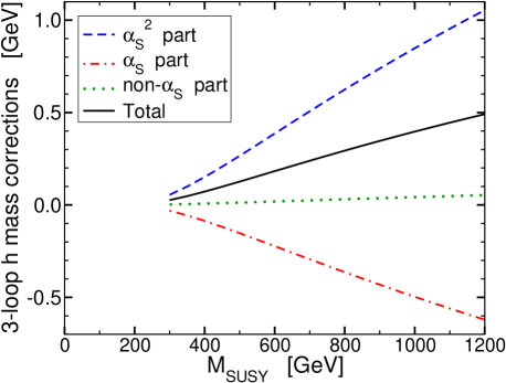
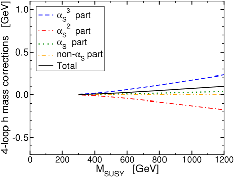
Figure 1: Leading-logarithm contributions to $M_{h}$ from 3 loops (left panel) and 4 loops (right panel), as a function of the common superpartner mass $M_{\rm SUSY}$. These results are due to the $L^{3}$ part of eq. (4.10) and the $L^{4}$ part of eq. (4.11), respectively, with separate contributions from the various powers of the MSSM QCD coupling and the total shown. The Higgs pole mass is taken to be $M_{h}=120$ GeV and $\tan\beta\gg 1$ and $\alpha_{S}^{(5),\overline{\rm MS}}(M_{Z})=0.118$ (in the five-quark effective Standard Model QCD theory) and top-quark pole mass $M_{t}=172$ GeV.

This illustrates the more general fact that the numerical magnitude of the three-loop correction depends on the way that perturbation theory is organized. Changing the renormalization scale or scheme, or re-expanding tree-level masses in one-loop and two-loop integral functions around pole masses, can and does move contributions between loop orders. For example, ref. Degrassi:2002fi found the result quoted in eq. (A.17) of the present paper, which yields a rather larger numerical magnitude for the three-loop correction, written in terms of Standard Model effective couplings evaluated at $Q=M_{t}$.

For comparison, the four-loop order leading logarithm ($L^{4}$) contributions are shown in the right panel of figure 1, using the same scale. As expected, these are quite small, and there is again a fortuitous partial cancellation between the leading and next-to-leading orders in $\alpha_{S}$.

The next-to-leading logarithm ($L^{2}$) contributions at three-loop order can be seen to depend on the top-squark mixing and other details, and are not depicted numerically here, although they can be significant. I expect that in application to real-world data, one will want to re-express the perturbative expansion by expanding tree-level masses in one-loop and two-loop kinematic integrals around the pole masses, as this will likely further improve the convergence of perturbation theory (see ref. Martin:2006ub for an analogous discussion for the gluino-squark system in supersymmetric QCD). This will add more terms to the next-to-leading parts of the three-loop contribution.

If supersymmetry is discovered and thoroughly explored at the LHC and a future linear collider, the mass of the lightest Higgs boson will present an important precision test of our understanding of the theory. The leading three-loop corrections will be important for this test. It should be emphasized that, at this writing, some two-loop contributions remain uncalculated, namely those involving purely electroweak couplings, which may turn out to be similarly important. These contributions cannot be captured adequately by the effective potential approximation, since some of the relevant self-energy diagrams contain a routing by which the external momentum does not go through any propagator with mass larger than $M_{Z}$ or $M_{h}$. Therefore, it will probably be necessary to evaluate those two-loop self-energy diagrams on-shell in order to reduce theoretical errors to an acceptable level.

Appendix: Comparison with other work

It is useful to check the correspondence of the preceding formulas with earlier special case results. For convenience, I focus on the two-loop results given in refs. EZ2 and ENHiggs , and the three-loop leading-log results of Degrassi:2002fi .

First, consider the approximations of refs. EZ2 :

$$|s_{\tilde{t}}c_{\tilde{t}}|\>=\>1/2;$$ (A.1)

$$m^{2}_{\tilde{t}_{1,2}}\>=\>M_{S}^{2}\mp m_{t}|X_{t}|;$$ (A.2)

$$m_{t}^{2},\>m_{t}|X_{t}|\>\ll\>M_{S}^{2};$$ (A.3)

$$m_{\tilde{g}}\>=\>m_{\tilde{b}_{L}}\>=\>m_{H}\>=\>|\mu|=M_{S},$$ (A.4)

but $|X_{t}|$ not necessarily small compared to $M_{S}$. Then the results above become:

$$c_{y_{t}} = \frac{4}{3}\bigl{[}1-{\rm Re}[X_{t}]/M_{S}+{\overline{\rm ln}}(M_{S}^{2})\bigr{]},$$ (A.5)

$$c^{\prime}_{y_{t}} = \frac{3}{4s_{\beta}^{2}}[(1+c_{\beta}^{2}){\overline{\rm ln}}(M_{S}^{2})-c_{\beta}^{2}/2],$$ (A.6)

$$c_{\lambda} = 12{\overline{\rm ln}}(M_{S}^{2})+12|X_{t}|^{2}/M_{S}^{2}-|X_{t}|^{4}/M_{S}^{4},\phantom{xxx}$$ (A.7)

$$c_{v} = |X_{t}|^{2}/4M_{\rm S}^{2},$$ (A.8)

$$c_{g_{3}} = 2{\overline{\rm ln}}(M_{S}^{2})-1/2,$$ (A.9)

in accord with the two-loop results found in eqs.(13)-(19) and (25) of ref. EZ2 . Note that the two-loop non-logarithmic parts in eqs. (16) and (17) of ref. EZ2 are not shown explicitly in the present paper; instead, the complete contributions up to two-loop order in SPM0206136 ; SPM0211366 ; SPM0405022 can be included by the procedure described at the end of section IV.

Next, consider the approximations of ref. ENHiggs , which involve a light right-handed top squark:

$$m_{\tilde{t}}^{2}\>=\>\begin{pmatrix}M_{L}^{2}+m_{t}^{2}&m_{t}X_{t}^{*}\\ m_{t}X_{t}&M_{R}^{2}+m_{t}^{2}\end{pmatrix};$$ (A.10)

$$m_{t}^{2},\>m_{t}|X_{t}|\>\ll\>M_{R}^{2}\>\ll\>M_{L}^{2};$$ (A.11)

$$m_{\tilde{g}}\>=\>m_{\tilde{b}_{L}}=m_{H}=|\mu|=M_{\rm L},$$ (A.12)

but $|X_{t}|$ not necessarily small compared to $M_{L}$. Then the results above become

$$c_{y_{t}} = \frac{1}{3}\bigl{[}1-8{\rm Re}[X_{t}]/M_{L}+4{\overline{\rm ln}}(M_{L}^{2})\bigr{]},$$ (A.13)

$$c^{\prime}_{y_{t}} = \frac{3}{8}\Bigl{(}1-\frac{2}{s_{\beta}^{2}}\Bigr{)}[1-2{\overline{\rm ln}}(M_{L}^{2})]-\frac{3|X_{t}|^{2}}{4M_{\rm L}^{2}},$$ (A.14)

$$c_{\lambda} = 6{\overline{\rm ln}}(M_{L}^{2})+6{\overline{\rm ln}}(M_{R}^{2})+\frac{12|X_{t}|^{2}}{M_{L}^{2}}\ln(M_{L}^{2}/M_{R}^{2})$$ (A.15)

$$+\frac{6|X_{t}|^{4}}{M_{L}^{4}}\bigl{[}2-\ln(M_{L}^{2}/M_{R}^{2})\bigr{]},$$

$$c_{v} = 3|X_{t}|^{2}/4M_{\rm L}^{2},$$ (A.16)

in agreement with the two-loop results of Appendix A and eqs. (B.8) and (C.12) and (C.13) in ref. ENHiggs . Note that ref. ENHiggs also explicitly identifies two-loop contributions enhanced by large logarithms $\ln(M_{L}^{2}/M_{R}^{2})$, which are not obtained in the approach used here except when they are also enhanced by a $\ln(M_{L}^{2}/m_{t}^{2})$. This is because ref. ENHiggs used a multi-stage effective field theory method, first decoupling left-handed top squarks and then right-handed top squarks. Also, the approach of ref. ENHiggs isolates the non-logarithmic two-loop effective potential contributions within the given approximation, which are not shown explicitly here. Again, in the approach of the present paper, the complete two-loop order results of refs. SPM0206136 ; SPM0211366 ; SPM0405022 can be included and consistently supplemented by the three-loop result as described at the end of section IV.

Now, consider the three-loop leading log result given in eq. (11) of Degrassi:2002fi , which assumes a single sparticle mass threshold at $M_{S}$ and $\tan\beta\gg 1$, and is given in terms of running $\overline{\rm MS}$ couplings evaluated at the top mass scale. In the notation of section III of the present paper, that result is:

$$M_{h}^{2} = \widehat{m}_{Z}^{2}+\widehat{y}_{t}^{4}\widehat{v}^{2}\Bigl{[}12\kappa L_{t}+\kappa^{2}L_{t}^{2}(-96\widehat{g}_{3}^{2}+18\widehat{y}_{t}^{2})$$ (A.17)

$$+\kappa^{3}L_{t}^{3}(736\widehat{g}_{3}^{4}-240\widehat{g}_{3}^{2}\widehat{y}_{t}^{2}-99\widehat{y}_{t}^{4})\Bigr{]},$$

where

$$L_{t}=\ln(M_{S}^{2}/m_{t}^{2}).$$ (A.18)

Now, in the leading-logarithm approximation, the translation of SM parameters evaluated at the top mass scale to the MSSM parameters evaluated at $M_{S}$ depends only the Standard Model one-loop renormalization group equations, and is independent of the $\overline{\rm MS}$ to $\overline{\rm DR}^{\prime}$ conversion and threshold corrections. One can write:

$$\widehat{g}_{3} = g_{3}\bigl{[}1+\kappa L_{t}(7g_{3}^{2}/2)+...\bigr{]},$$ (A.19)

$$\widehat{y}_{t} = y_{t}\bigl{[}1+\kappa L_{t}(4g_{3}^{2}-9y_{t}^{2}/4)$$ (A.20)

$$+\kappa^{2}L_{t}^{2}(22g_{3}^{4}-18g_{3}^{2}y_{t}^{2}+243y_{t}^{4}/32)+...\bigr{]},\phantom{xxx}$$

$$\widehat{v} = v\bigl{[}1+\kappa L_{t}(3y_{t}^{2}/2)$$ (A.21)

$$+\kappa^{2}L_{t}^{2}(6g_{3}^{2}y_{t}^{2}-9y_{t}^{4}/4)+...\bigr{]},$$

where the parameters on the left sides are evaluated at $Q=m_{t}$, and those on the right sides at $Q=M_{S}$. Plugging these into eq. (A.17) immediately yields the special form of eqs. (4.6)-(4.10) with only the leading logarithms and $s_{\beta}=1$:

$$M_{h}^{2} = m_{Z}^{2}+y_{t}^{4}v^{2}\Bigl{[}12\kappa L_{t}+\kappa^{2}L_{t}^{2}(96g_{3}^{2}-54y_{t}^{2})$$ (A.22)

$$+\kappa^{3}L_{t}^{3}(736g_{3}^{4}-672g_{3}^{2}y_{t}^{2}+90y_{t}^{4})\Bigr{]}.$$

This is more useful as a rough indicator of the sizes of theoretical errors due to three-loop effects than as an actual precise evaluation of $M_{h}$.

Acknowledgments: This work was supported by the National Science Foundation under Grant No. PHY-0456635.

References

(1)
“ATLAS detector and physics performance. Technical design report. Vol. 2,”
CERN-LHCC-99-15,
and V. Drollinger and A. Sopczak,
Eur. Phys. J. C 3, N1 (2001),
[hep-ph/0102342].
(2)
T. Abe et al. [American Linear Collider Working Group
Collaboration],
“Linear collider physics resource book for Snowmass 2001. 2: Higgs and
supersymmetry studies,”
[hep-ex/0106056].
(3)
J.A. Aguilar-Saavedra et al. [ECFA/DESY LC Physics Working Group
Collaboration],
“TESLA Technical Design Report Part III: Physics at an e+e- Linear
Collider,”
[hep-ph/0106315].
(4)
K. Abe et al. [ACFA Linear Collider Working Group Collaboration],
“Particle physics experiments at JLC,”
[hep-ph/0109166].
(5)
S.P. Li and M. Sher,
Phys. Lett. B 140, 339 (1984).
(6)
M.S. Berger,
Phys. Rev. D 41, 225 (1990).
(7)
H.E. Haber and R. Hempfling,
Phys. Rev. Lett. 66, 1815 (1991).
(8)
Y. Okada, M. Yamaguchi and T. Yanagida,
Prog. Theor. Phys. 85, 1 (1991);
Phys. Lett. B 262, 54 (1991).
(9)
J. Ellis, G. Ridolfi and F. Zwirner,
Phys. Lett. B 257, 83 (1991);
Phys. Lett. B 262, 477 (1991).
(10)
R. Barbieri, M. Frigeni and F. Caravaglios,
Phys. Lett. B 258, 167 (1991).
(11)
A. Yamada,
Phys. Lett. B 263, 233 (1991).
(12)
J.R. Espinosa and M. Quirós,
Phys. Lett. B 266, 389 (1991).
(13)
A. Brignole,
Phys. Lett. B 281, 284 (1992).
(14)
M. Drees and M.M. Nojiri,
Nucl. Phys. B 369, 54 (1992);
Phys. Rev. D 45, 2482 (1992).
(15)
K. Sasaki, M. Carena and C.E.M. Wagner,
Nucl. Phys. B 381, 66 (1992).
(16)
P.H. Chankowski, S. Pokorski and J. Rosiek,
Phys. Lett. B 274, 191 (1992);
Nucl. Phys. B 423, 437 (1994)
[hep-ph/9303309].
(17)
H.E. Haber and R. Hempfling,
Phys. Rev. D 48, 4280 (1993)
[hep-ph/9307201].
(18)
J. Kodaira, Y. Yasui and K. Sasaki,
Phys. Rev. D 50, 7035 (1994)
[hep-ph/9311366].
(19)
A. Yamada,
Z. Phys. C 61, 247 (1994).
(20)
R. Hempfling and A.H. Hoang,
Phys. Lett. B 331, 99 (1994)
[hep-ph/9401219].
(21)
J.A. Casas, J.R. Espinosa, M. Quirós and A. Riotto,
Nucl. Phys. B 436, 3 (1995)
[Erratum-ibid. B 439, 466 (1995)]
[hep-ph/9407389].
(22)
A. Dabelstein,
Z. Phys. C 67, 495 (1995)
[hep-ph/9409375].
(23)
M. Carena, J.R. Espinosa, M. Quiros and C.E.M. Wagner,
Phys. Lett. B 355, 209 (1995)
[hep-ph/9504316].
(24)
M. Carena, M. Quirós and C. Wagner,
Nucl. Phys. B 461, 407 (1996)
[hep-ph/9508343].
(25)
D.M. Pierce, J.A. Bagger, K.T. Matchev and R.J. Zhang,
Nucl. Phys. B 491, 3 (1997)
[hep-ph/9606211].
(26)
H.E. Haber, R. Hempfling and A.H. Hoang,
Z. Phys. C 75, 539 (1997)
[hep-ph/9609331].
(27)
S. Heinemeyer, W. Hollik and G. Weiglein,
Phys. Rev. D 58, 091701 (1998)
[hep-ph/9803277];
Phys. Lett. B 440, 296 (1998)
[hep-ph/9807423].
(28)
R.J. Zhang,
Phys. Lett. B 447, 89 (1999)
[hep-ph/9808299].
(29)
S. Heinemeyer, W. Hollik and G. Weiglein,
Comput. Phys. Commun. 124, 76 (2000)
[hep-ph/9812320];
M. Frank, S. Heinemeyer, W. Hollik and G. Weiglein,
[hep-ph/0202166];
T. Hahn, W. Hollik, S. Heinemeyer and G. Weiglein,
“Precision Higgs masses with FeynHiggs 2.2,”
[hep-ph/0507009].
(30)
S. Heinemeyer, W. Hollik and G. Weiglein,
Eur. Phys. J. C 9, 343 (1999)
[hep-ph/9812472].
(32)
J.R. Espinosa and R.J. Zhang,
Nucl. Phys. B 586, 3 (2000)
[hep-ph/0003246].
(33)
A. Pilaftsis and C.E.M. Wagner,
Nucl. Phys. B 553, 3 (1999)
[hep-ph/9902371].
(34)
M. Carena et al.,
Nucl. Phys. B 580, 29 (2000)
[hep-ph/0001002].
(35)
M. Carena, J.R. Ellis, A. Pilaftsis and C.E.M. Wagner,
Nucl. Phys. B 586, 92 (2000)
[hep-ph/0003180].
(36)
J.R. Espinosa and I. Navarro,
Nucl. Phys. B 615, 82 (2001)
[hep-ph/0104047].
(37)
G. Degrassi, P. Slavich and F. Zwirner,
Nucl. Phys. B 611, 403 (2001)
[hep-ph/0105096].
(38)
S. Heinemeyer,
Eur. Phys. J. C 22, 521 (2001)
[hep-ph/0108059].
(39)
M. Carena, J.R. Ellis, A. Pilaftsis and C.E.M. Wagner,
Nucl. Phys. B 625, 345 (2002)
[hep-ph/0111245].
(40)
A. Brignole, G. Degrassi, P. Slavich and F. Zwirner,
Nucl. Phys. B 631, 195 (2002)
[hep-ph/0112177];
Nucl. Phys. B 643, 79 (2002)
[hep-ph/0206101].
(41)
S.P. Martin,
Phys. Rev. D 66, 096001 (2002) [hep-ph/0206136];
Phys. Rev. D 65, 116003 (2002)
[hep-ph/0111209].
(42)
S.P. Martin,
Phys. Rev. D 67, 095012 (2003)
[hep-ph/0211366].
(43)
G. Degrassi, S. Heinemeyer, W. Hollik, P. Slavich and G. Weiglein,
Eur. Phys. J. C 28, 133 (2003)
[hep-ph/0212020].
(44)
M. Frank, S. Heinemeyer, W. Hollik and G. Weiglein,
“The Higgs boson masses of the complex MSSM: A complete one-loop
calculation,”
[hep-ph/0212037].
(45)
A. Dedes, G. Degrassi and P. Slavich,
Nucl. Phys. B 672, 144 (2003)
[hep-ph/0305127].
(46)
J.S. Lee et al,
Comput. Phys. Commun. 156, 283 (2004) [hep-ph/0307377].
(47)
S.P. Martin,
Phys. Rev. D 70, 016005 (2004)
[hep-ph/0312092].
(48)
S.P. Martin,
Phys. Rev. D 71, 016012 (2005)
[hep-ph/0405022].
The results in this paper are written in terms of two-loop integrals
reduced to basis integrals in
S.P. Martin,
Phys. Rev. D 70, 016005 (2004)
[hep-ph/0312092].
The basis integrals are in turn evaluated numerically by computer TSIL .
(49)
B.C. Allanach, A. Djouadi, J.L. Kneur, W. Porod and P. Slavich,
JHEP 0409, 044 (2004)
[hep-ph/0406166].
(50)
S. Heinemeyer,
Int. J. Mod. Phys. A 21, 2659 (2006)
[hep-ph/0407244].
(51)
S. Heinemeyer, W. Hollik, H. Rzehak and G. Weiglein,
Eur. Phys. J. C 39, 465 (2005)
[hep-ph/0411114].
(52)
W. Hollik and D. Stockinger,
Phys. Lett. B 634, 63 (2006)
[hep-ph/0509298].
(53)
M. Frank, T. Hahn, S. Heinemeyer, W. Hollik, H. Rzehak and G. Weiglein,
[hep-ph/0611326].
(54)
W. Siegel,
Phys. Lett. B 84, 193 (1979);
D.M. Capper, D.R.T. Jones and P. van Nieuwenhuizen,
Nucl. Phys. B 167, 479 (1980).
(55)
I. Jack et al,
Phys. Rev. D 50, 5481 (1994)
[hep-ph/9407291].
(57)
M.E. Machacek and M.T. Vaughn,
Nucl. Phys. B 249, 70 (1985);
Nucl. Phys. B 236, 221 (1984);
Nucl. Phys. B 222, 83 (1983).
(58)
C. Ford, I. Jack and D.R.T. Jones,
Nucl. Phys. B 387, 373 (1992)
[hep-ph/0111190].
(59)
S.P. Martin,
Phys. Rev. D 74, 075009 (2006)
[hep-ph/0608026].
(60)
S.P. Martin,
Phys. Rev. D 68, 075002 (2003) [hep-ph/0307101];
S.P. Martin and D.G. Robertson, “TSIL: a program for
the calculation of two-loop self-energy integrals”,
Comput. Phys. Commun. 174, 133 (2006),
[hep-ph/0501132].