Alberta Thy 20-06

Coulomb force correction to the decay $b\rightarrow c\bar{c}s$ in the threshold

K. Hasegawa

Department of Physics, University of Alberta, Edmonton, AB T6G 2J1, Canada

Abstract

We study the physical origins of the ${\cal O}(\alpha_{s})$ and ${\cal O}(\alpha_{s}^{2})$ corrections to the $\bar{c}-s$ current in the decay $b\rightarrow c\bar{c}s$ in the threshold region $\delta=(M_{b}-2m_{c})/2M_{b}\ll 1$. We obtain the corrections which are produced by the Coulomb force between the anti-charm and strange quarks. The Coulomb corrections $C_{F}\pi^{2}$ at ${\cal O}(\alpha_{s})$ and $-C_{F}^{2}\pi^{2}\mbox{ln}\ \delta$ at ${\cal O}(\alpha_{s}^{2})$ account for 300% and 120% of the corresponding terms in the Abelian-type perturbative corrections respectively. The differences between the Coulomb and perturbative corrections imply that other corrections which have other physical origins exist. We also check that the Wilson coefficient for the anomalous dimension of the $\bar{c}-s$ current reproduces the leading and the next-to-leading logarithmic terms in the perturbative corrections.

1 Introduction

Disagreement between the experimental measurements and the theoretical predictions for the branching ratio of the semi-leptonic decay of the B meson, $\mbox{BR}(B\to X\bar{l}\nu_{l})$, has been reported [1]. Because the non-perturbative corrections related to the confinement of the participating quarks inside the hadrons are at a level of a few percent [1], the branching ratio of the semi-leptonic decay is mainly determined by the decay rates of the three decay modes of the free $b$ quark decay, the semi-leptonic mode $b\rightarrow c\bar{l}\nu_{l}$, the non-leptonic mode with light quarks $b\rightarrow c\bar{u}d$, and the non-leptonic mode with an extra charm quark $b\rightarrow c\bar{c}s$. Here, the non-leptonic modes contribute to the branching ratio of the semi-leptonic decay through the total decay width of the $b$ quark. About 30% enhancement of the ${\cal O}(\alpha_{s})$ corrections to the $\bar{c}-s$ current in the non-leptonic mode $b\rightarrow c\bar{c}s$ has been obtained [2, 3, 4, 5, 6]. When the large enhancement at the ${\cal O}(\alpha_{s})$ level and the evolution of the renormalization group from the scale of the $W$ boson mass to that of the $b$ quark mass are taken into account, the significant disagreement with experiments vanishes [3, 4, 5, 7]. It has also been reported that the ${\cal O}(\alpha_{s}^{2})$ corrections to the non-leptonic mode $b\rightarrow c\bar{u}d$ remain in agreement with experiments [8]. At the present stage, the ${\cal O}(\alpha_{s}^{2})$ corrections to the other non-leptonic mode, $b\rightarrow c\bar{c}s$, becomes one of the main issues with the theoretical predictions of the semi-leptonic branching ratio. The ${\cal O}(\alpha_{s})$ correction to the $\bar{c}-s$ current in the mode $b\rightarrow c\bar{c}s$ is a monotonically increasing function of the mass of the charm quark, and the ratio of the ${\cal O}(\alpha_{s})$ correction to the tree-level rate diverges in the threshold region $\delta=(M_{b}-2m_{c})/2M_{b}\ll 1$ due to the logarithmic term $(\mbox{ln}\ \delta)$. Furthermore, although the fully analytic form of the ${\cal O}(\alpha_{s}^{2})$ corrections, including the charm mass dependence, has not been obtained, it is known that the ${\cal O}(\alpha_{s}^{2})$ corrections also contain the leading logarithmic terms $(\mbox{ln}\ \delta)^{2}$ and the next-to-leading logarithms $(\mbox{ln}\ \delta)$. We conjecture that the large corrections come from the threshold region and think it meaningful to elucidate the physical origins of the large corrections. With this goal in mind, in the present paper, we focus on the ${\cal O}(\alpha_{s})$ and ${\cal O}(\alpha_{s}^{2})$ corrections to the $\bar{c}-s$ current in the threshold region of the decay $b\rightarrow c\bar{c}s$ and estimate the quantum corrections which come from the two physical origins, the Coulomb force between the $\bar{c}$ and $s$ quarks, and the anomalous dimension of the $\bar{c}-s$ current.

It is well known that the Coulomb force between the proton and the electron produces the additional corrections to the tree-level decay rate of the neutron beta decay $n\to pe^{-}\nu_{e}$ (see, e.g, the textbook [9]). The wave function of the electron is distorted by the Coulomb force generated by the electromagnetic charge of the approximately static proton. The distorted wave function forms the Fermi function in the decay rate. Considering the Fermi function in the neutron beta decay, here we attempt to incorporate the effects of the Coulomb-like gluon exchanges between the $\bar{c}$ and $s$ quarks in the threshold region of the decay $b\rightarrow c\bar{c}s$. In Ref.[10] , it is pointed out that the Fermi function for the $\bar{c}-s$ current produces a next-to-leading logarithm in the ${\cal O}(\alpha_{s}^{2})$ corrections. However, in that work, the Fermi function is not introduced to the decay rate formula which contains the phase space integrals of the final states. We believe it is worthwhile to obtain an estimate of the effect of the Coulomb distortion of the strange quark in the decay rate formula in order to obtain the more precise predictions of the Coulomb corrections. Considering this point, the main purpose of the present paper is to incorporate the Fermi function into the decay $b\rightarrow c\bar{c}s$ and to obtain the corrections which are produced by the Coulomb force between the $\bar{c}$ and $s$ quarks in the threshold region. We then compare the Coulomb corrections with the Abelian parts of the perturbative corrections at the ${\cal O}(\alpha_{s})$ and ${\cal O}(\alpha_{s}^{2})$ levels. The other origin of the logarithmic terms is known. It is shown that the Wilson coefficients for the anomalous dimension of the heavy-light current, which is called the hybrid anomalous dimension, reproduce the leading logarithmic terms in the perturbative corrections of the two-body decay into one heavy and one light particle [11, 12, 13]. Furthermore, when the Wilson coefficients are improved by the non-logarithmic terms at ${\cal O}(\alpha_{s})$ in the perturbative corrections, the improved coefficient can produce the next-to-leading logarithmic terms in the ${\cal O}(\alpha_{s}^{2})$ corrections [14, 15, 16, 17]. In the present paper, we confirm that the leading and next-to-leading logarithms in the perturbative corrections to the decay rate $\Gamma(b\rightarrow c\bar{c}s)$ can also be reduced to the Wilson coefficients for the hybrid anomalous dimension.

The remainder of the present paper is organized as follows. In §2 we obtain the threshold expansion of the perturbative corrections at ${\cal O}(\alpha_{s})$ and ${\cal O}(\alpha_{s}^{2})$ in the decay $b\rightarrow c\bar{c}s$. In §3 we obtain the Coulomb force corrections and compare them with the Abelian parts of the perturbative corrections. In §4 we show that the Wilson coefficient for the hybrid anomalous dimension reproduces the leading and next-to-leading logarithmic terms in the perturbative corrections. In §5 we give a summary.

2 Results of the perturbative calculation

We start with the effective Lagrangian for the decay $b\rightarrow c\bar{c}s$,

$${\cal L}=-V_{cb}V_{cs}^{*}\frac{G_{F}}{\sqrt{2}}\bigr{[}\bar{\psi_{c}}\gamma^{\mu}(1-\gamma_{5})\psi_{b}\bigl{]}\bigr{[}\bar{\psi_{s}}\gamma_{\mu}(1-\gamma_{5})\psi_{c}\bigl{]}.$$ (1)

We first calculate the tree-level decay rate by using the ordinal decay rate formula

$$\Gamma(b\rightarrow c\bar{c}s)=\frac{1}{2M_{b}}\int\frac{d^{3}p_{c}}{(2\pi)^{3}}\frac{1}{2p_{c}^{0}}\frac{d^{3}p_{\bar{c}}}{(2\pi)^{3}}\frac{1}{2p_{\bar{c}}^{0}}\frac{d^{3}p_{s}}{(2\pi)^{3}}\frac{1}{2p_{s}^{0}}|{\cal M}|^{2}$$

$$(2\pi)^{4}\delta^{(4)}(p_{b}-p_{c}-p_{\bar{c}}-p_{s}),$$ (2)

where ${\cal M}$ is the invariant matrix and $M_{b}$ is the mass of the bottom quark. The momenta of the bottom, charm, anti-charm, and strange quarks are written $p_{b},p_{c},p_{\bar{c}}$, and $p_{s}$. The tree-level decay rate $\Gamma(b\rightarrow c\bar{c}s)_{0}$ is obtained as

$$\Gamma(b\rightarrow c\bar{c}s)_{0} = \Gamma_{\mu}\Biggl{[}\sqrt{1-4\epsilon^{2}}\bigl{(}1-14\epsilon^{2}-2\epsilon^{4}-12\epsilon^{6}\bigr{)}$$ (3)

$$\hskip 85.35826pt+24\epsilon^{4}(1-\epsilon^{4})\mbox{ln}\Biggl{(}\frac{1+\sqrt{1-4\epsilon^{2}}}{1-\sqrt{1-4\epsilon^{2}}}\Biggr{)}\Biggr{]},$$

where the ratio of the charm quark mass to the bottom quark mass is written $\epsilon=m_{c}/M_{b}$. The decay rate at $\epsilon=0$ is denoted by $\Gamma_{\mu}=N_{c}|V_{cb}|^{2}|V_{cs}|^{2}G_{F}^{2}M_{b}^{5}/(192\pi^{3})$, with $N_{c}=3$. We can also obtain the decay rate from the so-called ‘factorization formula’,

$$\Gamma(b\rightarrow c\bar{c}s)=|V_{cb}|^{2}|V_{cs}|^{2}G_{F}^{2}\int^{(M_{b}-m_{c})^{2}}_{m_{c}^{2}}\frac{dq^{2}}{(2\pi)}\ \sqrt{q^{2}}\ X^{\mu\nu}Y_{\mu\nu}.$$ (4)

Here, $X^{\mu\nu}$ and $Y_{\mu\nu}$ are defined as

$$\Gamma(b\rightarrow cW^{-}) = \epsilon_{\mu}^{\lambda*}(q)\epsilon_{\nu}^{\lambda}(q)X^{\mu\nu},$$ (5)

$$\Gamma(W^{-}\rightarrow\bar{c}s) = \epsilon_{\mu}^{\lambda}(q)^{*}\epsilon_{\nu}^{\lambda}(q)Y^{\mu\nu},$$ (6)

where $q$ and $\epsilon_{\mu}^{\lambda}(q)$ are the momentum and polarization vector of the $W$ gauge boson. When we calculate $X^{\mu\nu}$ and $Y^{\mu\nu}$ in Eqs. (5) and (6), we use the Lagrangians ${\cal L}=\bar{\psi_{c}}\gamma^{\mu}(1-\gamma_{5})\psi_{b}W_{\mu}^{+}$ and ${\cal L}=\bar{\psi_{s}}\gamma^{\mu}(1-\gamma_{5})\psi_{c}W_{\mu}^{-}$, respectively, where the coupling constants are normalized to unity. The mass squared of the $W$ boson, $q^{2}$, is the variable of integration in Eq. (4), and it runs over the region in which both of the decay processes $b\rightarrow cW^{-}$ and $W^{-}\rightarrow\bar{c}s$ can occur. We can calculate $X^{\mu\nu}$ at tree level as

$$X^{\mu\nu} = \frac{1}{4\pi}\frac{\sqrt{\lambda(M_{b}^{2},m_{c}^{2},q^{2})}}{M_{b}^{3}}\int\frac{d\Omega}{4\pi}$$ (7)

$$\biggl{[}2p_{b}^{\mu}p_{b}^{\nu}-p_{b}^{\mu}q^{\nu}-p_{b}^{\nu}q^{\mu}-g^{\mu\nu}M_{b}^{2}+g^{\mu\nu}(p_{b}\cdot q)-i\epsilon^{\alpha\mu\beta\nu}q_{\alpha}p_{b,\beta}\biggr{]},$$

where the variable $\Omega$ represents the direction of the momentum of the $W$ boson, and $\lambda$ is defined as $\lambda(a,b,c)=a^{2}+b^{2}+c^{2}-2(ab+bc+ca)$. We can also calculate $Y^{\mu\nu}$ at tree level as

$$Y^{\mu\nu}=-\frac{N_{c}}{4\pi\sqrt{q^{2}}}\bigl{[}A_{0}(q^{2}g^{\mu\nu}-q^{\mu}q^{\nu})-B_{0}q^{\mu}q^{\nu}\bigr{]},$$ (8)

where $A_{0}$ and $B_{0}$ are the transversal and longitudinal parts, respectively, in the $W$ boson decay. They are calculated as

$$A_{0}\biggl{(}\frac{\epsilon^{2}}{\omega^{2}}\biggr{)} = \frac{2}{3}\biggl{(}1-\frac{\epsilon^{2}}{\omega^{2}}\biggr{)}^{2}\biggl{(}1+\frac{\epsilon^{2}}{2\omega^{2}}\biggr{)},$$ (9)

$$B_{0}\biggl{(}\frac{\epsilon^{2}}{\omega^{2}}\biggr{)} = \frac{\epsilon^{2}}{\omega^{2}}\biggl{(}1-\frac{\epsilon^{2}}{\omega^{2}}\biggr{)}^{2},$$ (10)

where $\omega=\sqrt{q^{2}}/M_{b}$. Substituting Eqs. (7) and (8) into Eq. (4), we obtain the following form :

$$\Gamma(b\rightarrow c\bar{c}s) = 6\Gamma_{\mu}\int_{\epsilon^{2}}^{(1-\epsilon)^{2}}d\omega^{2}\sqrt{\lambda(1,\epsilon^{2},\omega^{2})}$$ (11)

$$\biggl{[}\omega^{2}(1+\epsilon^{2}-\omega^{2})A_{0}+\bigl{(}(1-\epsilon^{2})^{2}-(1+\epsilon^{2})\omega^{2}\bigr{)}\frac{A_{0}+B_{0}}{2}\biggr{]}.$$

Then, substituting Eqs.(9) and (10) into Eq.(11), we can obtain a result which coincides with that given in Eq. (3). Thus, we can reproduce the tree-level decay rate in Eq. (3) from the factorization formula (4). Since we focus on the threshold region of the decay $b\rightarrow c\bar{c}s$ in the present paper, we obtain the threshold expansion of the tree-level decay rate in Eq. (3) as

$$\Gamma(b\rightarrow c\bar{c}s)_{0}=\Gamma_{\mu}\frac{4096}{35}\delta^{7/2}\biggl{(}1-\frac{231}{66}\delta+\frac{1283}{264}\delta^{2}\cdots\biggl{)},$$ (12)

where the expansion parameter $\delta$ is defined as $\delta=1/2-\epsilon$.

Next, we consider the estimation of the QCD corrections to the decay $b\rightarrow c\bar{c}s$. In the present paper, we concentrate on the QCD corrections to the part of the decay $W^{-}\rightarrow\bar{c}s$ in the factorization formula (4). We write the decay rate including the quantum corrections to the $\bar{c}-s$ current as

$$\Gamma(b\rightarrow c\bar{c}s)=\Gamma_{0}\biggl{(}1+\frac{\alpha_{s}}{\pi}\Delta_{1}+\biggl{(}\frac{\alpha_{s}}{\pi}\biggr{)}^{2}\Delta_{2}\biggr{)},$$ (13)

where $\Delta_{1}$ and $\Delta_{2}$ are the ${\cal O}(\alpha_{s})$ and ${\cal O}(\alpha_{s}^{2})$ corrections. We write the ${\cal O}(\alpha_{s})$ and ${\cal O}(\alpha_{s}^{2})$ corrections to the transversal part $A_{0}$ in Eq. (8) as $A_{1}$ and $A_{2}$ and denote the sum of the transversal part as $A=A_{0}+A_{1}+A_{2}$. In the same way we write the longitudinal part as $B=B_{0}+B_{1}+B_{2}$. The ${\cal O}(\alpha_{s})$ corrections $A_{1}$ and $B_{1}$ are given as the functions of $z=\omega^{2}/\epsilon^{2}$ as [6]

$$A_{1} = \biggl{(}\frac{\alpha_{s}}{\pi}\biggr{)}C_{F}A_{0}\biggl{[}f_{1}(z)+\frac{2z}{2z+1}f_{2}(z)\biggr{]},$$ (14)

$$B_{1} = \biggl{(}\frac{\alpha_{s}}{\pi}\biggr{)}C_{F}B_{0}[f_{1}(z)-1],$$ (15)

where $C_{F}=4/3$ and $f_{1}(z)$ and $f_{2}(z)$ are given by

$$f_{1}(z) = \frac{13}{4}+2\mbox{Li }\biggl{(}\frac{1}{z}\biggr{)}+\mbox{ln}z\ \mbox{ln}\frac{z}{z-1}-\frac{3}{2}\ \mbox{ln}(z-1)+\mbox{ln}\frac{z}{z-1}+\frac{1}{z}\ \mbox{ln}(z-1)$$ (16)

$$+\frac{1}{z-1}\ \mbox{ln}z,$$

$$f_{2}(z) = -\frac{5}{2}-\frac{1}{z}-\frac{1}{z-1}+\biggl{(}\frac{z-1}{z}\biggr{)}\ \biggl{(}\frac{3}{2}+\frac{1}{2z}\biggr{)}\ \mbox{ln}(z-1)+\frac{z}{(z-1)^{2}}\ \mbox{ln}z.$$ (17)

Here, $\mbox{Li}(x)=-\int_{0}^{x}\mbox{ln}(1-t)dt/t$ is the standard dilogarithm function. Replacing $A_{0}$ and $B_{0}$ with $A_{1}$ and $B_{1}$, respectively, in Eq. (11), we evaluated the integrals numerically and obtained the form of $\Delta_{1}$ plotted as the solid curve in Fig. 1.

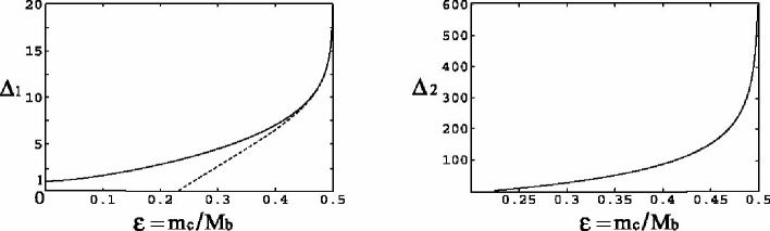
Figure 1: The corrections $\Delta_{1}$ and $\Delta_{2}$. In the plot of $\Delta_{1}$, the solid curve and the dashed curve represent the exact results and the first three terms in Eq. (22) in the threshold expansion, respectively. In the plot of $\Delta_{2}$, the solid curve represents the first three terms in Eq. (25).

From this graph, we can read off the value $\Delta_{1}=4.46$ at the reference point $\epsilon=0.3$, which produces the corrections $(\alpha_{s}/\pi)\Delta_{1}=0.28$ when we use the value $\alpha_{s}=0.2$. This enhancement by about 30% is also reported in Ref.[6] . In order to observe the ${\cal O}(\alpha_{s})$ corrections in the threshold region, we use the expansion parameter $\rho=1-1/z$ and expand $A_{1}$ and $B_{1}$ in Eqs. (14) and (15) up to the first three terms as

$$A_{1} = \biggl{(}\frac{\alpha_{s}}{\pi}\biggr{)}C_{F}\frac{\rho^{2}}{2}\biggl{[}\biggl{(}\frac{9}{2}-3L_{\rho}+\frac{2}{3}\pi^{2}\biggr{)}+\rho\biggl{(}-\frac{139}{18}+\frac{11}{3}L_{\rho}-\frac{2}{9}\pi^{2}\biggr{)}$$ (18)

$$\hskip 199.16928pt+\rho^{2}\biggl{(}-\frac{23}{18}+\frac{1}{3}L_{\rho}\biggr{)}\biggr{]},$$

$$B_{1} = \biggl{(}\frac{\alpha_{s}}{\pi}\biggr{)}C_{F}(1-\rho)\rho^{2}\biggl{[}\biggl{(}\frac{13}{4}-\frac{3}{2}L_{\rho}+\frac{1}{3}\pi^{2}\biggr{)}-3\rho+\rho^{2}\biggl{(}-\frac{35}{12}+\frac{1}{2}L_{\rho}\biggr{)}\biggr{]}.$$

These expansions coincide with the results of the perturbative calculations presented in Ref.[19] . Here, we define $L_{\rho}=\mbox{ln}\rho$. We change the variable of integration from $\omega^{2}$ to $u=(1/2-\omega)$ in Eq. (11) to obtain the threshold expansion. With $A_{1}$ and $B_{1}$ in Eqs. (18) and (LABEL:b1ex), we obtain the following threshold expansion :

$$\Gamma_{0}\biggl{(}\frac{\alpha_{s}}{\pi}\biggl{)}\Delta_{1} = 6\Gamma_{\mu}\int_{-\delta}^{\delta}du(1-2u)\ \sqrt{u+\delta}\sqrt{(1-\delta+u)(1+\delta-u)(2-\delta-u)}$$ (21)

$$\biggl{[}\Bigl{(}\frac{1}{2}-u\Bigr{)}^{2}(1-\delta+u+\delta^{2}-u^{2})A_{1}+$$

$$\biggl{(}\Bigl{(}\frac{3}{4}+\delta-\delta^{2}\Bigr{)}^{2}-\Bigl{(}\frac{1}{2}-u\Bigr{)}^{2}\Bigl{(}\frac{5}{4}-\delta+\delta^{2}\Bigr{)}\biggr{)}\frac{A_{1}+B_{1}}{2}\biggr{]}$$

$$= \Gamma_{\mu}\ \biggl{(}\frac{\alpha_{s}}{\pi}\biggr{)}\ \biggl{[}\biggl{(}\frac{387008}{1155}+\frac{16384}{315}\pi^{2}-\frac{16384}{35}\mbox{ln}2-\frac{8192}{35}L_{\delta}\biggr{)}\delta^{7/2}+$$

$$\biggl{(}-\frac{125825888}{45045}-\frac{8192}{45}\pi^{2}+\frac{1040384}{315}\mbox{ln}2+\frac{520192}{315}L_{\delta}\biggr{)}\delta^{9/2}+$$

$$\biggl{(}\frac{22449032}{15015}+\frac{2627584}{10395}\pi^{2}-\frac{727040}{99}\mbox{ln}2-\frac{363520}{99}L_{\delta}\biggr{)}\delta^{11/2}$$

$$\hskip 199.16928pt+\cdots\biggr{]}.$$

Here, we define $L_{\delta}=\mbox{ln}\delta$. Dividing the quantity in Eq. (21) by that in Eq. (12), we obtain the threshold expansion for $\Delta_{1}$ as

$$\Delta_{1} = \biggl{(}\frac{6047}{2112}+\frac{4}{9}\pi^{2}-4\ \mbox{ln}2-2L_{\delta}\biggr{)}+\biggl{(}-\frac{570307}{41184}+\frac{128}{9}\ \mbox{ln}2+\frac{64}{9}L_{\delta}\biggr{)}\delta$$ (22)

$$+\biggl{(}-\frac{11236399}{226512}+\frac{640}{99}\ \mbox{ln}2+\frac{320}{99}L_{\delta}\biggr{)}\delta^{2}+\cdots.$$

We plot the first three terms in Eq. (22) as the dashed curve in Fig. 1. We can see in the plot that although the first three terms in Eq. (22) are sufficient to reproduce the approximate value in the region $\epsilon\gtrsim 0.45$, they are not sufficient at the realistic reference point $\epsilon=0.3$.

Finally, we obtain the threshold expansion of the ${\cal O}(\alpha_{s}^{2})$ corrections. Their analytic forms, $A_{2}$ and $B_{2}$, are not known. The first three terms in the threshold expansions of $A_{2}$ and $B_{2}$ are obtained as [19]

$$A_{2} = \biggl{(}\frac{\alpha_{s}}{\pi}\biggr{)}^{2}C_{F}\frac{2}{3}\rho^{2}(C_{F}\Delta_{A}^{v}+C_{A}\Delta_{NA}^{v}+T_{R}N_{L}\Delta_{L}^{v}+T_{R}\Delta_{H}^{v}),$$ (23)

$$B_{2} = \biggl{(}\frac{\alpha_{s}}{\pi}\biggr{)}^{2}C_{F}(1-\rho)\rho^{2}(C_{F}\Delta_{A}^{s}+C_{A}\Delta_{NA}^{s}+T_{R}N_{L}\Delta_{L}^{s}+T_{R}\Delta_{H}^{s}),$$ (24)

where the explicit forms of $\Delta_{A}^{v}$, $\Delta_{NA}^{v}$, and so on are given in Ref.[19] . Here, we define the coefficients as $C_{F}=4/3,\ C_{A}=3$ and $T_{R}=1/2,$ and we count the number of light quarks as $N_{L}=3$ in the present $b$ quark decay. Using Eqs. (11), (12), (23) and (24), we obtain the threshold expansion for $\Delta_{2}$ as

$$\Delta_{2} = \biggl{[}\frac{3367549}{76032}+\frac{42877}{12672}\pi^{2}-\frac{2}{81}\pi^{4}-\frac{444217}{6336}\mbox{ln}2-\frac{188}{27}\pi^{2}\mbox{ln}2+26(\mbox{ln}2)^{2}$$ (25)

$$\ -\frac{444217}{12672}L_{\delta}-\frac{91}{27}\pi^{2}L_{\delta}+26\mbox{ln}2\ L_{\delta}+\frac{13}{2}L_{\delta}^{2}-\frac{70}{3}\zeta(3)\biggr{]}+$$

$$\biggl{[}-\frac{1471797053}{8895744}+\frac{41175}{9152}\pi^{2}+\frac{7578347}{28512}\mbox{ln}2+\frac{464}{243}\pi^{2}\mbox{ln}2-\frac{1088}{9}(\mbox{ln}2)^{2}+$$

$$\ \ \frac{7578347}{57024}L_{\delta}+\frac{160}{243}\pi^{2}L_{\delta}-\frac{1088}{9}\mbox{ln}2L_{\delta}-\frac{272}{9}L_{\delta}^{2}+\frac{104}{27}\zeta(3)\biggr{]}\delta+$$

$$\biggl{[}-\frac{29171145503}{3669494400}-\frac{202553411}{12231648}\pi^{2}+\frac{10217309}{141570}\mbox{ln}2+\frac{5552}{891}\pi^{2}\mbox{ln}2+$$

$$\ \ \frac{60608}{891}(\mbox{ln}2)^{2}+\frac{10217309}{283140}L_{\delta}+\frac{2656}{891}\pi^{2}L_{\delta}+\frac{60608}{891}\mbox{ln}2\ L_{\delta}+$$

$$\ \frac{15152}{891}L_{\delta}^{2}+\frac{200}{33}\zeta(3)\biggr{]}\delta^{2}+\cdots.$$

We plot the first three terms in Eq.(25) in Fig. 1. We can see in the plot that the divergences in the threshold region are more rapid than the divergences of $\Delta_{1}$ in Eq.(22), due to the existence of the terms $L_{\delta}^{2}$. Although the corrections in Eq. (25) at the reference point $\epsilon=0.3$ are not valid, we read it as $\Delta_{2}=25.2$ for order estimation. Using this value, the decay rate is estimated as $\Gamma(b\rightarrow c\bar{c}s)=\Gamma_{0}(1+0.28+0.10)$, where the second and third terms are the $O(\alpha_{s})$ and $O(\alpha_{s}^{2})$ corrections in Eq. (13) with $\alpha_{s}=0.2$. Then, in order to make the magnitudes of the corrections in the threshold region concrete, we take the values $\Delta_{1}=13.3$ and $\Delta_{2}=324$ at the reference point $\epsilon=0.49$. We estimate the corrections at the reference point as $\Gamma(b\rightarrow c\bar{c}s)=\Gamma_{0}(1+0.85+1.31)$. This estimation shows that the sum of the first few terms in the perturbation series at the threshold cannot produce a valid approximation.

3 Coulomb force correction

In this section we obtain the corrections which are produced by the Coulomb force between the anti-charm and strange quarks in the final state of the decay $b\rightarrow c\bar{c}s$. Our method to obtain the Coulomb force corrections is to replace the plane wave function of the strange quark by the wave function in the presence of the Coulomb potential. This method is used to incorporate the effect of the Coulomb distortion of the electron plane wave by the electromagnetic charge of the proton in the neutron beta decay rate [9]. The decay rate formula in Eq. (2) is not suitable for the distorted wave function by the Coulomb potential because the distorted wave function is not a momentum eigenfunction and we cannot extract the momentum conservation law which is expressed as the delta functions in Eq. (2). We choose a normalization of one particle per volume $V$ for the plane waves in this section. Then we start the inclusion of the Coulomb corrections with the decay rate formula as

$$d\Gamma=2\pi|\langle f|\hat{H}_{\mbox{int}}(t=0)|i\rangle|^{2}\ \delta\biggl{(}M-\sum_{i=1}^{n}p_{i}^{0}\biggr{)}\prod_{i=1}^{n}\frac{d^{3}p_{i}}{(2\pi)^{3}}\mbox{V}.$$ (26)

Here, the interaction Hamiltonian is defined as $\hat{H}_{\mbox{int}}(t)=\int d^{3}x\hat{{\cal H}}_{\mbox{int}}(\vec{x},t)$, where $\hat{{\cal H}}_{\mbox{int}}$ is interaction Hamiltonian density and $M$ is the mass of the initial particle. Since the initial and final states of the decays are energy eigenstates, we can factor out the delta function which gives the energy conservation law. Using the interaction Lagrangian in Eq. (1) for the present decay, we can write the transition matrix as

$$\langle c\bar{c}s|\hat{H}_{\mbox{int}}(t=0)|b\rangle=V_{cb}V_{cs}^{*}\frac{G_{F}}{\sqrt{2}}\int d^{3}x\bigr{[}\bar{\psi_{c}}\gamma^{\mu}(1-\gamma_{5})\psi_{b}\bigl{]}\bigr{[}\bar{\psi_{s}}\gamma_{\mu}(1-\gamma_{5})\psi_{\bar{c}}\bigl{]}.$$

(27)

In the ordinal perturbation theory, we use the plane waves for the participating particles as

$$\psi_{b}^{r}(\vec{x}) = \sqrt{\frac{1}{V}}u^{r}(\vec{p}_{b}=0),\ \ \psi_{c}^{r^{\prime}}(\vec{x})=\sqrt{\frac{E_{c}+m_{c}}{2E_{c}V}}u^{r^{\prime}}(\vec{p}_{c})e^{+i\vec{p}_{c}\cdot\vec{x}},$$

$$\psi_{\bar{c}}^{s}(\vec{x}) = \sqrt{\frac{E_{\bar{c}}+m_{c}}{2E_{\bar{c}}V}}v^{s}(\vec{p}_{\bar{c}})e^{-i\vec{p}_{\bar{c}}\cdot\vec{x}}\ \ \mbox{and}\ \ \psi_{s}^{s^{\prime}}(\vec{x})=\sqrt{\frac{1}{2V}}u^{s^{\prime}}(\vec{p}_{s})e^{+i\vec{p}_{s}\cdot\vec{x}},$$ (28)

where the spinors of the particle and anti-particle are defined as

$$u^{s}(\vec{p})=\left(\begin{array}[]{c}\chi^{s}\\ \frac{\vec{\sigma}\cdot\vec{p}}{E+m}\chi^{s}\end{array}\right)\ \ \mbox{and}\ \ v^{s}(\vec{p})=(-s)\left(\begin{array}[]{c}\frac{\vec{\sigma}\cdot\vec{p}}{E+m}\chi^{-s}\\ \chi^{-s}\end{array}\right),$$ (33)

with $s=1$ for the up spin and $s=-1$ for the down spin. Here we employ the standard Dirac representation, in which $\gamma^{0}$ is a diagonal matrix and the plane waves are normalized to one particle per volume $V$ as $\int_{V}d^{3}x\ \psi^{s}(x)^{\dagger}\psi^{s^{\prime}}(x)=\delta_{s,s^{\prime}}$. In order to obtain the Coulomb corrections, we have the following two approximations. The first approximation is to ignore the small Pauli components $(\vec{\sigma}\cdot\vec{p})\chi^{s}/(E+m)$ in the wave functions of the nonrelativistic charm and anti-cham quarks, because their small components do not contribute to the leading term of the threshold expansion. The second one is to replace the wave function of the strange quark in Eq. (28) with its value at the origin as

$$\psi_{s}^{s^{\prime}}(\vec{x})\simeq\psi_{s}^{s^{\prime}}(\vec{x}=0),$$ (34)

because the contributions of the wave function at a radius far from the origin can be ignored in the first term of the threshold expansion. These two approximations are justified by the fact that the resultant decay rate coincides with the first term in the exact decay rate at tree level in Eq. (12), as shown below. Taking advantage of the approximation in Eq. (34), we replace the plane wave at the origin with the wave function in the Coulomb potential at the origin. We briefly review the solution of Dirac equation with the Coulomb potential (see, e.g, the textbook Ref. [20] ). Here we keep the finite mass of the strange quark unless stated otherwise. We solve the Dirac equation,

$$\biggl{(}i\gamma_{\mu}\partial^{\mu}-|e|QA_{\mu}\gamma^{\mu}-m\biggr{)}\psi(x)=0,$$ (35)

with the Coulomb potential $A_{0}=-|e|Q_{s}/r$ and $A_{i}=0$. To solve this equation we can use the general form of the wave function in a spherically symmetric potential,

$$\Psi_{E,+}^{j,j_{3}}(\vec{x},t)=\left(\begin{array}[]{c}f(r){\cal Y}_{j,\ l}^{j_{3},(+)}\\ g(r){\cal Y}_{j,\ l+1}^{j_{3},(-)},\end{array}\right)e^{-iEt},$$ (38)

where ${\cal Y}_{j,\ l}^{j_{3},(\pm)}$ represents the spinor-spherical harmonics, and the total angular momentum is defined as $j=l+1/2$, with the orbital angular momentum $l$. Although we have one more choice for the wave function, in which the orbital angular momentum of the upper two components is larger than that of the lower two components by unity, we use the wave function in Eq. (38), because the s-wave of the particle (strange quark) in the present case contributes to the Coulomb corrections. We obtain the solutions of the radial parts with the continuum energy spectrum as

$$\left(\begin{array}[]{r}f_{l}(r)\\ g_{l}(r)\end{array}\right)=N_{l}e^{-ikr}(2kr)^{\gamma-1}\times$$ (41)

$$\hskip 14.22636pt\left(\begin{array}[]{c}\sqrt{E+m}\bigl{[}{}_{1}F_{1}(\xi,1+2\gamma,2ikr)+\frac{\xi}{l+1-ia}{}_{1}F_{1}(\xi+1,1+2\gamma,2ikr)\bigr{]}\\ \sqrt{E-m}\bigl{[}{}_{1}F_{1}(\xi,1+2\gamma,2ikr)-\frac{\xi}{l+1-ia}{}_{1}F_{1}(\xi+1,1+2\gamma,2ikr)\bigr{]}\end{array}\right),$$ (44)

where ${}_{1}F_{1}$ is the Kummer function and we have $\gamma=\sqrt{(l+1)^{2}-\alpha_{0}^{2}},\ \xi=\gamma+i\nu,\ \nu=\alpha_{0}E/k,\ a=\alpha_{0}m/k$ and $\alpha_{0}=-|e|^{2}QQ_{s}$. Using the normalization condition

$$\int d^{3}x\ \Psi_{E}^{j,j_{3}}(\vec{x})^{\dagger}\Psi_{E}^{j^{\prime},j_{3}^{\prime}}(\vec{x})=\delta_{j,j^{\prime}}\delta_{j_{3},j_{3}^{\prime}}\frac{E\pi}{k^{2}}\delta(k-k^{\prime}),$$ (45)

we fix the normalization constant as

$$N_{l}=e^{\pi\nu/2}\cdot\frac{|\Gamma(1+\gamma+i\nu)|}{|\Gamma(1+2\gamma)|},$$ (46)

where $\Gamma(z)$ is the Gamma function. We can rewrite the solutions of the radial parts in Eq. (44) near the origin as

$$\left(\begin{array}[]{r}f_{l}(r=R)\\ g_{l}(r=R)\end{array}\right)\simeq N_{l}e^{-ikr}(2kR)^{\gamma-1}\left(\begin{array}[]{c}\sqrt{E+m}\bigl{[}1+\frac{\xi}{1-ia}\bigr{]}\\ \sqrt{E-m}\bigl{[}1-\frac{\xi}{1-ia}\bigr{]}\end{array}\right),$$ (51)

where we define the radius near the origin as $R\simeq 0$. When the Coulomb potential is switched off and the Coulomb wave is reduced to a free spherical wave, the inner product of the wave functions in Eq. (38) with $j=1/2$ near the origin is given by

$$\Psi_{E}^{j=1/2,j_{3}}(\vec{x})^{\dagger}\Psi_{E}^{j=1/2,j_{3}}(\vec{x})\bigl{|}_{r=R,\ \alpha_{0}=0}=\frac{E+m}{4\pi},$$ (52)

which differs from that of the plane waves, $\psi^{s}(x)^{\dagger}\psi^{s}(x)=1/V$. In order to replace the plane wave in Eq. (34) with the Coulomb-distorted wave in Eq. (38) near the origin in a consistent way, we modify the normalization constant of the Coulomb wave in Eq. (46) as

$$\Psi_{E}^{j,j_{3}}(\vec{x})^{\mbox{new}}\bigl{|}_{r=R}=\sqrt{\frac{4\pi}{(E+m)V}}\Psi_{E}^{j,j_{3}}(\vec{x})\bigl{|}_{r=R}.$$ (53)

For this purpose, here we define the Fermi function as

$$\mbox{F}(E,\alpha_{0})=\frac{|\Psi_{E}^{j,j_{3}}(\vec{x},\alpha_{0})|^{2}}{|\Psi_{E}^{j,j_{3}}(\vec{x},\alpha_{0}=0)|^{2}}\Biggl{|}_{r=R},$$ (54)

with $R\simeq 0$. Using Eqs. (38), (46), and (51), we obtain the explicit form of the Fermi function as

$$\mbox{F}(E,\alpha_{0})=4\frac{E+m\gamma_{0}}{E+m}\cdot(2kR)^{2(\gamma_{0}-1)}\cdot e^{\pi\nu}\cdot\frac{|\Gamma(\gamma_{0}+i\nu)|^{2}}{|\Gamma(1+2\gamma_{0})|^{2}},$$ (55)

with the relations $E=\sqrt{m^{2}+k^{2}}$ and $\gamma_{0}=\sqrt{1-\alpha_{0}^{2}}$. Hereafter, we omit the mass of the strange quark again and write the energy of the strange quark as $E_{s}=|\vec{p}_{s}|$. Substituting the plane waves in Eq. (28) into Eq. (27), except for the strange quark, and using the renormalized Coulomb wave in Eq. (53) for the strange quark, we obtain the transition matrix element as

$$\langle f|\hat{H}_{\mbox{int}}(t=0)|i\rangle = V_{cb}V_{cs}^{*}\frac{\sqrt{2}G_{F}}{V}(2\pi)^{3}\delta^{3}(\vec{p}_{c}+\vec{p}_{\bar{c}})\bigl{[}\delta_{r,r^{\prime}}j^{0}(\bar{c}s)$$ (56)

$$\hskip 113.81102pt+(\chi^{r^{\prime}\dagger}\sigma^{i}\chi^{r})j^{i}(\bar{c}s)\bigr{]}$$

$$= \langle f|\hat{H}_{\mbox{int}}|i\rangle_{V}+\langle f|\hat{H}_{\mbox{int}}|i\rangle_{A},$$ (57)

where $\langle f|\hat{H}_{\mbox{int}}|i\rangle_{V}$ and $\langle f|\hat{H}_{\mbox{int}}|i\rangle_{A}$ are defined as the first and second terms in Eq. (56), referring to the vector and the axial vector parts of the bottom-charm current, respectively. We write the anti-charm and strange quark current as $j^{\mu}(\bar{c}s)=\bar{\Psi}_{s}\gamma_{\mu}L\psi_{\bar{c}}=\bar{\Phi}_{s}\gamma_{\mu}\phi_{\bar{c}}$, where the left-handed fields are written as $\phi_{\bar{c}}=L\psi_{\bar{c}}$ and $\Phi^{s}=L\Psi_{E}^{j,j_{3}\mbox{new}}$, with the projection operator $L=(1-\gamma_{5})/2$. We average the square of Eq. (57) over the spins and obtain the contributions of the vector and axial vector parts as

$$\frac{1}{2}\sum_{r,r^{\prime},s,s^{\prime}}|\langle f|\hat{H}_{\mbox{int}}|i\rangle_{V}|^{2} = |V_{cb}V_{cs}|^{2}\frac{G_{F}^{2}}{V^{2}}\frac{(2\pi)^{3}\delta^{3}(\vec{p}_{c}+\vec{p}_{\bar{c}})}{V}\ \mbox{F}(E_{s},\alpha_{0}),$$ (58)

$$\frac{1}{2}\sum_{r,r^{\prime},s,s^{\prime}}|\langle f|\hat{H}_{\mbox{int}}|i\rangle_{A}|^{2} = |V_{cb}V_{cs}|^{2}\frac{G_{F}^{2}}{V^{2}}\frac{(2\pi)^{3}\delta^{3}(\vec{p}_{c}+\vec{p}_{\bar{c}})}{V}\ 3\ \mbox{F}(E_{s},\alpha_{0}),$$ (59)

where the interference term of the vector and axial vector parts does not contribute to the spin-averaged decay rate. When we derive Eqs. (58) and (59), we use the formulae $\sum_{s}\phi_{\bar{c}}^{s}(x)\phi_{\bar{c}}^{s}(x)^{\dagger}\simeq L/2V$ and $\sum_{s}\Phi^{s}(\vec{x})^{\dagger}\Phi^{s}(\vec{x})\bigl{|}_{r=R}=F(E_{s},\alpha_{0})/V$. Substituting Eqs. (58) and (59) into Eq. (26), we obtain the decay rate including the Fermi function $\Gamma(b\rightarrow c\bar{c}s)^{c}$ as

$$\Gamma(b\rightarrow c\bar{c}s)^{c}=768\ \Gamma_{\mu}\int_{0}^{\delta}dzz^{2}(1-2z)\sqrt{\delta-z-\delta^{2}+z^{2}}\cdot\mbox{F}(E_{s},\alpha_{0}),$$ (60)

where the variable of integration is defined as $z=E_{s}/2M_{b}$. We compute only the contribution to first order in $\delta$ and obtain the decay rate as

$$\Gamma(b\rightarrow c\bar{c}s)^{c}=\Gamma_{0}^{c}\biggl{[}1+\pi\alpha_{0}+\biggl{(}\frac{1019}{210}-\gamma_{e}+\frac{\pi^{2}}{3}-\mbox{ln}\bigl{(}M_{b}R\delta\bigr{)}-4\mbox{ln}2\biggr{)}\alpha_{0}^{2}\biggr{]}.$$

(61)

Here, we have used the expansion of the Fermi function in the coupling constant, $\mbox{F}(E,\alpha_{0})=1+\pi\alpha_{0}+(\pi^{2}/3+3-\gamma_{e}-\mbox{ln}(2ER))\alpha_{0}^{2}+\cdots$, and written the tree-level rate as $\Gamma_{0}^{c}=\Gamma_{\mu}(4096/35)\delta^{7/2}$, which coincides with the first term in Eq. (12). Here, $\gamma_{e}\simeq 0.577$ is Euler’s constant. Since the Coulomb corrections originate in the effects of the Coulomb-like gluon exchanges between the $\bar{c}$ and $s$ quarks, we can expect that the ${\cal O}(\alpha_{0})$ and ${\cal O}(\alpha_{0}^{2})$ corrections in Eq. (61) are included in the Abelian-type one- and two-loop diagrams shown in Fig. 2.

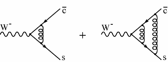
Figure 2: The Abelian-type diagrams which include the Coulomb-like gluon exchanges between the anti-charm and strange quarks.

In the correspondence, we can introduce the strong coupling constant as $\alpha_{0}=C_{F}\alpha_{s}$ and rewrite the series in Eq. (61) as

$$\frac{\Gamma(b\rightarrow c\bar{c}s)^{c}}{\Gamma_{0}^{c}} = 1+C_{F}\pi^{2}\biggr{(}\frac{\alpha_{s}}{\pi}\biggl{)}+\biggl{(}\frac{1019}{210}-\gamma_{e}+\frac{\pi^{2}}{3}-\mbox{ln}\bigl{(}M_{b}R\delta\bigr{)}-4\mbox{ln}2\biggr{)}$$ (62)

$$\hskip 170.71652pt\times\ C_{F}^{2}\pi^{2}\biggr{(}\frac{\alpha_{s}}{\pi}\biggl{)}^{2}.$$

Here we compare the corrections in Eq. (62) with the abelian part of the perturbative corrections in Eqs. (22) and (25). In the comparison we assume that the correspondence of terms is categorized according to the powers of the quantities, $\pi$, $\zeta(3)$, and logarithmic function. For example, the $\pi^{2}L_{\delta}$ term at ${\cal O}(\alpha_{s}^{2})$ in Eq. (62) is compared with the $\pi^{2}L_{\delta}$ term in the abelian part of the perturbative corrections in Eq. (25), rather than with the $L_{\delta}$ term. The coefficient $C_{F}\pi^{2}$ in the ${\cal O}(\alpha_{s})$ correction is three times larger than the similar $\pi^{2}$ term, $4\pi^{2}/9$, in Eq. (22). We conjecture that this difference is compensated for other corrections which have the other physical origins. At ${\cal O}(\alpha_{s}^{2})$, we extract the Abelian part from $\Delta_{2}$ in Eq. (25) by taking only $\Delta_{A}^{v}$ and $\Delta_{A}^{s}$ in Eqs. (23) and (24) and thereby obtain the first term as

$$\Delta_{2}^{\mbox{abel}} = C_{F}^{2}\biggl{[}\frac{119005}{22528}+\frac{1091}{2816}\pi^{2}+\frac{1}{90}\pi^{4}-\frac{16381}{2816}\mbox{ln}2-\frac{2}{3}\pi^{2}\mbox{ln}2+\frac{9}{2}(\mbox{ln}2)^{2}$$ (63)

$$-\frac{16381}{5632}L_{\delta}-\frac{5}{6}\pi^{2}L_{\delta}+\frac{9}{2}\mbox{ln}2\ L_{\delta}+\frac{9}{8}L_{\delta}^{2}-3\ \zeta(3)\biggr{]}+\cdots.$$

The term $-C_{F}^{2}\pi^{2}L_{\delta}$ in the ${\cal O}(\alpha_{s}^{2})$ corrections in Eq. (62) accounts for 120% of the similar $\pi^{2}L_{\delta}$ term, $-(5/6)C_{F}^{2}\pi^{2}L_{\delta}$, in Eq. (63). Because the $L_{\delta}^{2}$ and $L_{\delta}$ terms are singular at the threshold, these terms are not cancelled by other non-logarithmic terms. Based on the assumption that the terms are categorized according to $L_{\delta}$, $\pi^{2}$, and so on, we conjecture that the sum of the Coulomb corrections and other $\pi^{2}L_{\delta}$ corrections, which come from other physical origins in the Abelian theory, is $-(5/6)C_{F}^{2}\pi^{2}L_{\delta}$ in Eq. (63). The numerical impact of the Coulomb corrections, however, is not clear at the moment. The differences among the other terms, $1019\pi^{2}/210,\ \pi^{4}/3,$ and $-4\pi^{2}\mbox{ln}2$, at the ${\cal O}(\alpha_{s}^{2})$ in Eq. (62) and the corresponding terms in Eq. (63) are large. Although the Coulomb corrections do not contain terms of the forms $\mbox{ln}2,(\mbox{ln}2)^{2},L_{\delta},\mbox{ln}2L_{\delta},L_{\delta}^{2},\mbox{and}\ \zeta(3)$, the perturbative corrections do contain such terms. Further, the Coulomb corrections contain $\gamma_{e}$, while the perturbative corrections do not. We also believe that these differences are compensated for the other corrections.

4 Hybrid anomalous dimension

In this section, we show that the leading and next-to-leading logarithmic terms in the first order of the threshold expansions in Eqs. (22) and (25) originate in the anomalous dimension of the heavy-light $\bar{c}-s$ current $j=\bar{q}\Gamma Q$ in the heavy quark effective field theory (HQET), which is called the hybrid anomalous dimension [11]. Here, $q$ is a massless quark field, $Q$ is a heavy quark field in HQET, which satisfies the relation $Q=\gamma^{0}Q$, and $\Gamma$ represents the Dirac gamma matrices. First, solving the renormalization group equation

$$\biggl{(}\mu\frac{d}{d\mu}-\gamma_{h}(\alpha_{s}(\mu))\biggr{)}{\cal C}(\mu,M)=0,$$ (64)

we obtain the Wilson coefficient for the hybrid anomalous dimension as

$${\cal C}(\mu,M)={\cal C}(M,M)\exp\biggl{[}-\int^{\alpha_{s}^{(n_{l})}(\mu)}_{\alpha_{s}^{(n_{l})}(M)}\frac{\gamma_{h}(\alpha_{s})}{2\beta(\alpha_{s})}\frac{d\alpha_{s}}{\alpha_{s}}\biggr{]},$$ (65)

where the hybrid anomalous dimensions in HQET are given in Refs.[11, 12, 13, 14] and [21] as

$$\gamma_{h}=\gamma_{h}^{(0)}\frac{\alpha_{s}}{4\pi}+\gamma_{h}^{(1)}\biggl{(}\frac{\alpha_{s}}{4\pi}\biggr{)}^{2},$$ (66)

with $\gamma_{h}^{(0)}=-4$ and $\gamma_{h}^{(1)}=-\frac{254}{9}+\frac{20}{9}n_{l}-\frac{56}{27}\pi^{2}$. The beta function are given by

$$\beta = \beta_{0}\frac{\alpha_{s}}{4\pi}+\beta_{1}\biggl{(}\frac{\alpha_{s}}{4\pi}\biggr{)}^{2},$$ (67)

with $\beta_{0}=11-(2/3)n_{l}$ and $\beta_{1}=102-(38/3)n_{l}$. The hybrid anomalous dimension in HQET does not depend on the structure of the gamma matrices $\Gamma$. We write the initial condition in Eq. (65) as ${\cal C}(M,M)$, which depends on the structure $\Gamma$. In order to deal with the universal part in Eq. (65), we set the initial condition as ${\cal C}(M,M)=1$ hereafter. Valid initial conditions are introduced later through the matching coefficients. Using Eqs. (66) and (67), we obtain ${\cal C}(\mu,M)$ in Eq. (65) as

$${\cal C}(E_{s},m_{c})=\biggl{[}\frac{\alpha_{s}(E_{s})}{\alpha_{s}(m_{c})}\biggr{]}^{-\frac{\gamma_{h}^{(0)}}{2\beta_{0}}}\exp\Biggl{[}-\frac{\gamma_{h}^{(0)}}{8\pi\beta_{0}}\Biggl{(}\frac{\gamma_{h}^{(1)}}{\gamma_{h}^{(0)}}-\frac{\beta_{1}}{\beta_{0}}\Biggr{)}(\alpha_{s}(E_{s})-\alpha_{s}(m_{c}))\Biggr{]},$$ (68)

where we write $\mu$ as the threshold momentum $E_{s}$, like the energy of the strange quark in the presently considered decay, $b\rightarrow c\bar{c}s$, and $M$ as a heavy quark mass $m_{c}$, like the mass of the charm quark. Furthermore, we substitute $\alpha_{s}(E_{s})$ to Eq. (68) with the running coupling constant up to two-loop order,

$$\alpha_{s}(E_{s})=\frac{\alpha_{s}(m_{c})}{1+\alpha_{s}(m_{c})\frac{\beta_{0}}{2\pi}\log\frac{E_{s}}{m_{c}}+\alpha_{s}(m_{c})^{2}\frac{\beta_{1}}{8\pi^{2}}\log\frac{E_{s}}{m_{c}}},$$ (69)

and obtain the square of the Wilson coefficient in Eq. (68) as the following series in powers of the strong coupling constant $\alpha_{s}(m_{c})$ :

$${\cal C}^{2}(E_{s},m_{c}) = 1+\biggl{(}\frac{\alpha_{s}(m_{c})}{\pi}\biggr{)}\biggl{[}\frac{\gamma_{h}^{(0)}}{2}\mbox{ln}\ \frac{E_{s}}{m_{c}}\biggr{]}$$ (70)

$$+ \biggl{(}\frac{\alpha_{s}(m_{c})}{\pi}\biggr{)}^{2}\biggl{[}\frac{1}{8}\gamma_{h}^{(0)}(\gamma_{h}^{(0)}-\beta_{0})\biggl{(}\mbox{ln}\ \frac{E_{s}}{m_{c}}\biggr{)}^{2}+\frac{\gamma_{h}^{(1)}}{8}\biggl{(}\mbox{ln}\ \frac{E_{s}}{m_{c}}\biggr{)}\biggr{]}.$$

The leading logarithmic terms in the ${\cal O}(\alpha_{s})$ and ${\cal O}(\alpha_{s}^{2})$ corrections in Eq. (70) with $n_{l}=3$ coincide with those in the perturbative corrections in Eq. (22) and (25) when $\delta$ is replaced with $E_{s}/m_{c}$. This agreement shows that the leading logarithmic terms in the perturbative corrections come from the hybrid anomalous dimension. By contrast, the next-to-leading logarithmic term at ${\cal O}(\alpha_{s}^{2})$ does not coincide with that in Eq. (25). This disagreement between the next-to-leading logarithmic terms is natural for the following two reasons. The first reason is that the next-to-leading logarithms in the transversal part, $A/A_{0}$, and the longitudinal part, $B/B_{0}$, in the factorization formula (11) are different, while the leading logarithmic terms are the same. The second reason is that although the product of the leading logarithmic term and the non-logarithmic terms at ${\cal O}(\alpha_{s})$ can produce the next-to-leading logarithmic terms at ${\cal O}(\alpha_{s}^{2})$, the square of the Wilson coefficient in Eq. (70) does not contain non-logarithmic terms at ${\cal O}(\alpha_{s})$. In connection with the first of these reasons, the relations between $A/A_{0}$, $B/B_{0}$ and the universal part, $R(\rho)$, are given by [17]

$$\frac{A(\rho)}{A_{0}(\rho)} = C_{v}(m_{c})^{2}R(\rho),$$ (71)

$$\frac{B(\rho)}{B_{0}(\rho)} = \biggl{[}\frac{\bar{m}_{c}(m_{c})}{m_{c}}C_{s}(m_{c})\biggr{]}^{2}R(\rho),$$ (72)

where the matching coefficients are obtained as [22]

$$C_{v}(m_{c}) = 1-C_{F}\biggl{(}\frac{\alpha_{s}(m_{c})}{\pi}\biggr{)},$$ (73)

$$C_{s}(m_{c}) = 1+\frac{C_{F}}{2}\biggl{(}\frac{\alpha_{s}(m_{c})}{\pi}\biggr{)},$$ (74)

$$\frac{\bar{m}_{c}(m_{c})}{m_{c}} = 1-\frac{4}{3}\biggl{(}\frac{\alpha_{s}(m_{c})}{\pi}\biggr{)}.$$ (75)

Using Eqs. (9) and (18) and the leading and next-to-leading logarithmic terms in (23), we can extract the universal part $R(\rho)$ in Eq. (71) as

$$R(\rho) = 1+\biggl{(}\frac{\alpha_{s}(m_{c})}{\pi}\biggr{)}\biggl{[}-2L_{\rho}+\frac{17}{3}+\frac{4}{9}\pi^{2}\biggr{]}+\biggl{(}\frac{\alpha_{s}(m_{c})}{\pi}\biggr{)}^{2}$$ (76)

$$\times\biggl{[}\biggl{(}\frac{15}{2}-\frac{n_{l}}{3}\biggr{)}L_{\rho}^{2}+\biggl{(}-\frac{1657}{36}-\frac{97}{27}\pi^{2}+n_{l}\Bigl{(}\frac{13}{6}+\frac{4}{27}\pi^{2}\Bigr{)}\biggr{)}L_{\rho}\biggr{]},$$

which is consistent with Eq. (72). In connection to the second reason stated above, regarding the lack of non-logarithmic terms, we consider the non-logarithmic terms at ${\cal O}(\alpha_{s})$ in Eq. (76) and introduce the following factor at the scale of the threshold momentum $E_{s}$ :

$$D(E_{s})=1+\biggl{(}\frac{\alpha_{s}(E_{s})}{\pi}\biggr{)}\ \biggl{(}\frac{17}{3}+\frac{4}{9}\pi^{2}\biggr{)}.$$ (77)

The relation between $\alpha_{s}(E_{s})$ and $\alpha_{s}(m_{c})$ appearing here is given in Eq. (69). When the coefficient ${\cal C}^{2}(E_{s},m_{c})$ is improved by the factor $D(E_{s})$, it coincides with the universal part in Eq. (76), up to the next-to-leading logarithms at ${\cal O}(\alpha_{s}^{2})$, as

$${\cal C}^{2}(E_{s},m_{c})\cdot D(E_{s})=R\biggl{(}\rho=\frac{E_{s}}{m_{c}}\biggr{)}.$$ (78)

This means that the next-to-leading logarithmic terms in Eq. (25) can be reduced to the hybrid anomalous dimension and the running coupling constant in Eq. (69).

5 Summary

We have studied the physical origins of the corrections to the $\bar{c}-s$ current of the decay $b\rightarrow c\bar{c}s$ at the threshold. We first obtained the ${\cal O}(\alpha_{s})$ and ${\cal O}(\alpha_{s}^{2})$ perturbative corrections in Eqs. (22) and (25), respectively. Second, we obtained the corrections in Eq. (62), which are produced by the Coulomb force between the $\bar{c}$ and $s$ quarks. The Coulomb corrections, $C_{F}\pi^{2}$ at ${\cal O}(\alpha_{s})$ and $-C_{F}^{2}\pi^{2}\mbox{ln}\ \delta$ at ${\cal O}(\alpha_{s}^{2})$, account for 300% and 120% of the terms with the same forms in the Abelian parts of the perturbative corrections, respectively. The differences among the other terms in the ${\cal O}(\alpha_{s}^{2})$ corrections in Eq. (62) and the perturbative corrections of the same form are large. These differences should be compensated by other corrections which have other physical origins. We finally confirmed that the Wilson coefficient for the hybrid anomalous dimension reproduces the leading logarithmic terms in the perturbative corrections. We also confirmed that when the Wilson coefficient is improved by the non-logarithmic terms in the ${\cal O}(\alpha_{s})$ perturbative corrections, the improved coefficient can produce the next-to-leading logarithms in the ${\cal O}(\alpha_{s}^{2})$ perturbative corrections. We have identified three challenging problems in the present paper. The first problem is to reproduce the Coulomb corrections in Eq. (62) with perturbative calculations. In such calculation we should calculate only the loop diagrams shown in Fig 2 and extract only the soft-gluon contributions in the loop integrals. The second problem is to determine the accuracy of the method used to incorporate the Coulomb force corrections in §3. Solving this problem, we will be able to identify those terms that come from the Coulomb force corrections with the higher precision. The last problem is to find the relations between the two next-to-leading logarithmic terms of the Coulomb corrections in Eq. (62) and the Wilson coefficient for the hybrid anomalous dimension in Eq. (76). We should observe only the Abelian part of the hybrid anomalous dimension. Although the two next-to-leading logarithmic terms may originate in the soft and hard regions of the loop momentum, respectively, these relations are not trivial. We need more sophisticated studies to reveal these relations.

Acknowledgment

I would like to thank A. Pak for the valuable discussions. This work is supported by the fund for the Science and Engineering Research Canada.

References

• [1] I. Bigi, B. Blok, M. A. Shifman and A. Vainshtein, Phys. Lett. B 323 (1994), 408.
• [2] Q. Hokim and X. Y. Pham, Phys. Lett. B 122 (1983), 297.
• [3] E. Bagan, P. Ball, V. M. Braun and P. Gosdzinsky, Nucl. Phys. B 432 (1994), 3.
• [4] E. Bagan, P. Ball, V. M. Braun and P. Gosdzinsky, Phys. Lett. B 342 (1995), 362.
• [5] E. Bagan, P. Ball, B. Fiol and P. Gosdzinsky, Phys. Lett. B 351 (1995), 546.
• [6] M. B. Voloshin, Phys. Rev. D 51 (1995), 3948.
• [7] M. Neubert and C.T. Sachrajda, Nucl. Phys. B 483 (1997), 339.
• [8] A. Czarnecki, M. Slusarczyk and F. Tkachov Phys. Rev. Lett. 96 (2006), 171803.
• [9] E. J. Konopinski, The theory of beta radioactivity, Oxford university press, (1966), 403 p.
• [10] M. B. Voloshin, Int. J. Mod. Phys. A11 (1996), 4931.
• [11] M. B. Voloshin and M. A. Shifman, Sov. J. Nucl. Phys. 45 (1987), 292.
• [12] H. D. Politzer and M. B. Wise, Phys. Lett. B 206 (1988), 681.
• [13] H. D. Politzer and M. B. Wise, Phys. Lett. B 208 (1988), 504.
• [14] X. Ji and M. J. Musolf, Phys. Lett. B 257 (1991), 409.
• [15] D. J. Broadhurst and A. G. Grozin, Phys. Lett. B 274 (1992), 421.
• [16] E. Bagan, P. Ball, V. M. Braun, and H. G. Dosch, Phys. Lett. B 278 (1992), 457.
• [17] K. G. Chetyrkin and M. Steinhauser, Eur. Phys. J. C 21 (2001), 319.
• [18] G. Altarelli and S. Petrarca, Phys. Lett. B 261 (1991), 303.
• [19] A. Czarnecki and K. Melnikov, Phys. Rev. D 66 (2002), 011502.
• [20] F. J. Yndurain, Relativistic quantum mechanics and introduction to field theory, Springer, Berin, Germany, (1996), 332 p.
• [21] K. G. Chetyrkin and A. G. Grozin, Nucl. Phys. B 666 (2003), 289.
• [22] D. J. Broadhurst and A. G. Grozin, Phys. Rev. D 52 (1995), 4082.