Tensor and vector formulations of
resonance effective theory

Abstract

The main idea of the first order formalism is demonstrated on a toy example of spin-0 particle. The full formalism for spin-1 is applied to the vector formfactor of the pion and its high-energy behaviour is studied.

12.39.Fe, 12.40.Vv

1 Introduction

Recently, a considerable progress in the resonance saturation of the $O(p^{6})$ low energy constants (LECs) of the chiral perturbation theory ($\chi PT$) Lagrangian has been made. While a systematic classification of the relevant operator basis entering the large $N_{C}$ $QCD$ motivated Lagrangian of the chiral resonance theory ($\chi RT$) along with the formal resonance saturation of the $O(p^{6})$ LECs was given in [1], a phenomenological analysis for the symmetry breaking sector and a numerical estimate of the vector resonance contribution was discussed in detail in [2]. The importance of the vector resonances is established in the $O(p^{4})$ case, where whenever the vector resonances contribute, they dominate [3]. Note however, that the field-theory formulation of this sector of $\chi RT$ is not unique. The reason is that spin-1 resonances can be described using various types of fields, the most common ones in this context are the vector Proca fields and antisymmetric tensor fields (both formalisms will be discussed briefly in Section 2). Physical equivalence of various formulation of the spin-1 sector of $\chi RT$ at the order $O(p^{4})$ was studied already in the seminal paper [4], leading to the necessity to append additional contact terms to the Proca field $\chi RT$ Lagrangian in order to ensure both the formal equivalence with the antisymmetric tensor description (meaning equality of the correlators) and the physical one (to satisfy the high energy constraints dictated by $QCD$). At the $O(p^{6})$, the situation is more complex [5]. To obtain complete formal equivalence, one needs to add an infinite number of terms with increasing chiral order (to the contrary to $O(p^{4})$ case not only contact terms but also terms with explicit resonance fields). This infinite tower of operators can be truncated, provided we confine ourselves to the saturation of the $O(p^{6})$ LECs or provided we require equality of the $n$-point correlators up to some $n_{\max}$ only (see [5] for details). Even in such a case, however, both formalisms are in a sense incomplete, because generally some contributions to the $O(p^{6})$ LECs are still missing in both of them and have to be added by hand (for the tensor formalism this was made in [1] and [2] by means of the comparison with Proca field one). The necessity of additional terms might be required by the high energy $QCD$ constraints [1], however, the exhausting analysis is still missing here.

In [5], another possibility to describe spin-1 resonances has been discussed, which gives automatically all the contributions to the $O(p^{6})$ LECs known from the both formalisms mentioned above and which is in some sense a synthesis of them. Within this formalism, the spin-1 particles are described by a pair of vector and antisymmetric tensor fields which satisfy the first order equations of motion.

The aim of this paper is to demonstrate the main idea of this first order formalism using a toy example (see Section 3) and also to illustrate the application of the full formalism in the concrete case of the vector formfactor of the pion (see Section 4).

2 Description of vector resonances

Let us start with a brief review of two standard representations for the $1^{--}$ resonances. The first one, known from textbooks, is the familiar Proca field formalism; the (nonet) vector degree of freedom is represented by means of Lorentz vector $V_{\mu}^{a}$ (using Gell-Mann and unit matrices we have $V_{\mu}=\lambda^{a}V_{\mu}^{a}/\sqrt{2}$). The free field Lagrangian is given by

$$\mathcal{L}^{P}_{0}=-\tfrac{1}{4}\langle V_{\mu\nu}V^{\mu\nu}-2M_{V}^{2}V_{\mu}V^{\mu}\rangle\,,$$ (1)

where $V_{\mu\nu}=\partial_{\mu}V_{\nu}-\partial_{\nu}V_{\mu}$ and $\langle\ldots\rangle$ represents a trace in the flavour space.

The second formalism uses an antisymmetric tensor $R^{a}_{\mu\nu}$ with

$$\mathcal{L}^{T}_{0}=-\tfrac{1}{2}\langle\partial^{\lambda}R_{\lambda\mu}\partial_{\nu}R^{\nu\mu}-\tfrac{1}{2}M_{V}^{2}R_{\mu\nu}R^{\mu\nu}\rangle\,.$$ (2)

As follows from the equations of motion, this choice of the Lagrangian implies that the $R^{ij}$ degrees of freedom do not propagate. It could be shown that these two Lagrangians are equivalent (at least at the classical level).

The interactions with the Goldstone bosons follow from the symmetry properties of the underlying theory ($QCD$). Resonances transform as nonet under the $U(3)_{V}$ in the non-linear realization of chiral symmetry. The full Lagrangian can be constructed using the standard chiral building blocks of this non-linear realization together with the resonance fields. The leading order is represented by monomials which are linear in the resonance fields and chiral blocks are fixed by the standard ChPT counting scheme. These leading order monomials were first studied in [4, 6] and [3] for Proca and tensor formalism, respectively.

Integrating out the resonances one can study directly their influence in the sector of Goldstone bosons by saturation of low energy constants of $\chi PT$. This can also tell us what is the order of resonance nonet from the point of view of $\chi PT$; one gets: $O(p^{3})$ for $V^{\mu}$ and $O(p^{2})$ for $R^{\mu\nu}$. Having this powercounting one can construct further higher order terms; for this we refer to [6, 1, 2] (see also [5] and references therein).

As mentioned in Introduction, for a given order the equivalence between $\mathcal{L}^{P}$ and $\mathcal{L}^{T}$ is lost. One can ask which formalism is more appropriate to describe the vector resonances. Intuitively, due to the lower counting and thus richer structure, one would vote for tensor formalism (e.g. in Proca formalism we have no contribution to $O(p^{4})$ LECs). The situation is, however, more complicated. The point is that, even in this case, one is forced to fix extra contact terms (i.e. terms without resonances) in order to make the theory consistent. For instance (cf. [1]) at the order $O(p^{6})$, the Froissart bound applied to the $\pi^{0}$ Compton scattering amplitude calculated within the tensor formalism requires to add one such contact term. What is, however, interesting is that this term arises naturally in Proca formalism. It would be therefore useful to formulate the resonance theory in a way which would take advantages of both formalisms at once. This can be done using the first order formalism with the (free) Lagrangian of the form

$$\mathcal{L}^{PT}_{0}=\frac{1}{4}M_{V}^{2}\left\langle R_{\mu\nu}R^{\mu\nu}\right\rangle+\frac{1}{2}M_{V}^{2}\left\langle V_{\mu}V^{\mu}\right\rangle-\frac{1}{2}M_{V}\left\langle V_{\mu\nu}R^{\mu\nu}\right\rangle\,,$$ (3)

which was introduced in [5].

3 First order formalism

In order to avoid cumbersome expressions with lots of indices, let us demonstrate the main ideas of the first order formalism using a toy example of the noninteracting neutral massive spin-zero particles instead of the nonet of spin-1 resonances. The former case shares all the main qualitative features with the latter and due to its relative simplicity it suits well for our illustrative purpose.

Spin-zero particles are usually described in terms of the real massive scalar field with the Lagrangian

$$\mathcal{L}_{\phi}=\frac{1}{2}\left(\partial\phi\right)^{2}-\frac{1}{2}M^{2}\phi^{2}\,.$$ (4)

At the classical level, the corresponding Klein-Gordon equation is equivalent to a pair of first order equations for scalar and vector fields $\phi$ and $V_{\mu}$

$$\partial\phi-MV=0,\qquad\partial\cdot V+M\phi=0\,,$$ (5)

which can be derived from the “mixed” first order Lagrangian

$$\mathcal{L}_{\phi V}=MV\cdot\partial\phi-\frac{1}{2}M^{2}\phi^{2}-\frac{1}{2}M^{2}V^{2}=MV\cdot\partial\phi-\mathcal{H}_{\phi V}\,.$$ (6)

Here $\mathcal{H}_{\phi V}$ is the formal Legendre transformation of the Lagrangian $\mathcal{L}_{\phi}$ with respect to the derivatives $\partial_{\mu}\phi$ expressed in terms of its “canonically adjoint variables” $V_{\mu}M=\partial\mathcal{L}_{\phi}/\partial\partial^{\mu}\phi=\partial_{\mu}\phi$.

On the other hand, eliminating $\phi$ from (5) we get

$$\partial_{\mu}\partial\cdot V+M^{2}V_{\mu}=0\,,$$ (7)

which can be derived from the Lagrangian

$$\mathcal{L}_{V}=\frac{1}{2}\left(\partial\cdot V\right)^{2}-\frac{1}{2}M^{2}V^{2}\,.$$ (8)

This corresponds to an alternative and somewhat unusual possibility of description of the free neutral massive spin-zero particles. The Lagrangian $\mathcal{L}_{\phi V}$ can be in a sense interpreted as an interpolation between the two possibilities represented by the Lagrangians $\mathcal{L}_{\phi}$ and $\mathcal{L}_{V}$. At the quantum level $\mathcal{L}_{V}$ leads to the (covariant) propagator

$$\mathrm{i}\Delta_{F}^{V}(p)_{\mu\nu}=\frac{\mathrm{i}}{M^{2}}\left(\frac{p_{\mu}p_{\nu}}{p^{2}-M^{2}}-g_{\mu\nu}\right)\,,$$ (9)

which differs from the propagator of the field $\partial_{\mu}\phi/M$ derived from $\mathcal{L}_{\phi}$ by the presence of the contact term $\text{$\sim$}g_{\mu\nu}$. This means that including the interaction the descriptions based on $\mathcal{L}_{\phi}$ and $\mathcal{L}_{V}$ are not generally equivalent, unless additional contact terms are introduced. This situation is quite analogous to the case of Proca and tensor formalisms for spin-one particles [5].

The Lagrangian $\mathcal{L}_{\phi V}$ gives, besides the standard scalar propagator and $\Delta_{F}^{V}(p)_{\mu\nu}$ propagator also the “mixed” one

$$\mathrm{i}\Delta_{F}^{\phi V}(p)_{\mu}=\mathrm{i}\Delta_{F}^{V\phi}(-p)_{\mu}=\frac{\mathrm{i}}{p^{2}-M^{2}}\frac{\mathrm{i}p_{\mu}}{M}\,,$$ (10)

which is a novel feature of this formalism.

Let us now add interaction with external sources (which mimic the chiral building blocks here), i.e. to (4), (8) and (6) we add

$$\mathcal{L}_{\phi}^{\text{int}}=j\phi-\frac{1}{M}J\cdot\partial\phi;\quad\mathcal{L}_{V}^{\text{int}}=-\frac{1}{M}j\partial\cdot V+J\cdot V;\quad\mathcal{L}_{\phi V}^{\text{int}}=j\phi+J\cdot V$$ (11)

and suppose $j=O(p^{2})$, $J=O(p^{3})$. Integrating out the fields $\phi$ and/or $V$ up to the order $O(p^{6})$ we find out that in the case of first order formalism

$$\mathcal{L}_{\phi V}^{\text{eff}}=\frac{1}{2M^{2\,}}j^{2}+\frac{1}{2M^{4}}\left(\partial j\right)^{2}+\frac{1}{M^{3}}J\cdot\partial j+\frac{1}{2M^{2\,}}J^{2}.$$ (12)

The scalar field formalism misses the $O(p^{6})$ contribution $\frac{1}{2M^{2\,}}J^{2}$, while the vector field formalism includes this term, however it does not yield any contribution of the order $O(p^{4})$. The situation here is just analogous to the little bit more complicated case of the spin-1 resonances (cf. [5]).

4 Example: vector formfactor

Let us demonstrate the first order formalism for vector resonances on the example of vector formfactor defined as:

$$\langle\phi^{b}(p_{1})\phi^{c}(p_{2})|V^{\mu,a}|0\rangle=\mathcal{F}(q^{2})f^{abc}(p_{2}-p_{1})^{\mu}\,.$$

Here $\phi$s represent the Goldstone bosons and $q^{\mu}=(p_{1}+p_{2})^{\mu}$. Using the concrete form of the interaction Lagrangian and the Feynman rules given in [5] we get at the tree level

$$\mathcal{F}(q^{2})=1-\frac{f_{V}g_{V}}{F^{2}}\frac{q^{4}}{q^{2}-M_{V}^{2}}-\frac{F_{V}G_{V}}{F^{2}}\frac{q^{2}}{q^{2}-M_{V}^{2}}+\frac{F_{V}g_{V}+f_{V}G_{V}}{M_{V}F^{2}}\frac{q^{4}}{q^{2}-M_{V}^{2}}\,,$$

where the independent terms are in the one-to-one correspondence with Fig.1.

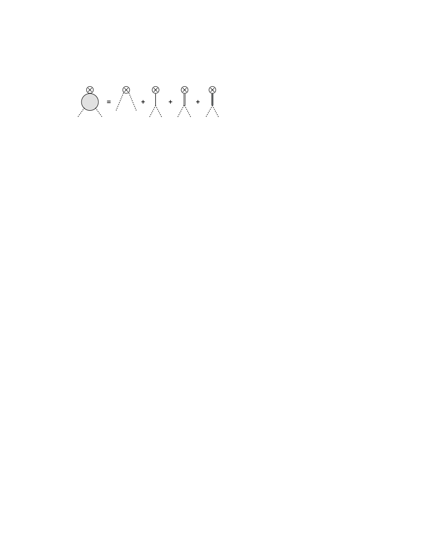
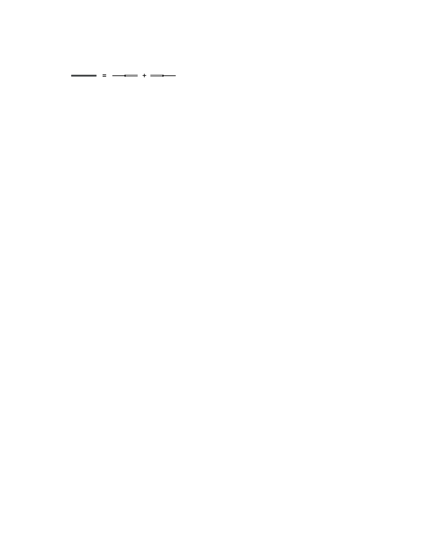
Figure 1: Diagram representation of the vector formfactor. Single line stands for Proca propagator, double line represents tensor propagator and dash lines correspond to Goldstone bosons. Filled line is the combination of mixed propagators: as defined in [5].

High energy conditions requires that the formfactor vanishes for $q^{2}\rightarrow\infty$. This implies the following conditions at the leading order in $1/N_{C}$:

$$F_{V}G_{V}=F^{2}\,,\qquad g_{V}F_{V}(f_{V}M_{V}-F_{V})=F^{2}f_{V}\,.$$ (13)

In the same way, imposing the short-distance constraints of $VVP$ correlator we get $f_{V}=0$ (for details see [5]) and the last condition of (13) simplifies to $g_{V}=0$.

5 Conclusion

In this paper, we have briefly discussed various ways of the field-theoretical descriptions of the spin-1 resonances. Besides the most common Proca and antisymmetric tensor field formalisms we have also assumed the new first order formalism introduced recently in [5]. Typical features of the latter have been illustrated using a toy example of the spin-0 particles. This simplification shares all the qualitative features with the spin-1 case: (i) description using a pair of fields with different Lorentz transformation properties, (ii) Feynman rules with mixed propagators and (iii) richer structure of the effective action obtained by means of integrating out the heavy fields. It might be interesting to further investigate the relevance of this formalism for the description of spin-0 resonances within $\chi RT$.

As an illustration of the first order formalism for spin-1 resonances we have explicitly calculated the vector formfactor of pion and discussed the consistency of the result with high energy behaviour. This supplies us with simple conditions without necessity of adding further contact terms. Moreover using the short-distance constraints of $VVP$ correlator (cf. [5]), the same result as in tensor formalism is obtained.

References

- [1] V. Cirigliano, G. Ecker, M. Eidemuller, R. Kaiser, A. Pich and J. Portoles, Nucl. Phys. B 753 (2006) 139.
- [2] K. Kampf and B. Moussallam, Eur. Phys. J. C 47 (2006) 723.
- [3] G. Ecker, J. Gasser, A. Pich and E. de Rafael, Nucl. Phys. B 321 (1989) 311.
- [4] G. Ecker, J. Gasser, H. Leutwyler, A. Pich and E. de Rafael, Phys. Lett. B 223 (1989) 425.
- [5] K. Kampf, J. Novotny and J. Trnka, arXiv:hep-ph/0608051; to appear in Eur. Phys. J. C.
- [6] J. Prades,Z. Phys. C 63 (1994) 491 [Erratum-ibid. C 11 (1999) 571].