Chiral symmetry patterns of excited mesons with the Coulomb-like linear confinement.

Abstract

The spectrum of $\bar{q}q$ mesons in a model where the only interaction is a linear Coulomb-like instantaneous confining potential is studied. The single-quark Green function as well as the dynamical chiral symmetry breaking are obtained from the Schwinger-Dyson (gap) equation. Given the dressed quark propagator, a complete spectrum of ”usual” mesons is obtained from the Bethe-Salpeter equation. The spectrum exhibits restoration of chiral and $U(1)_{A}$ symmetries at large spins and/or radial excitations. This property is demonstrated both analytically and numerically. At large spins and/or radial excitations higher degree of degeneracy is observed, namely all states with the given spin fall into reducible representations $[(0,1/2)\oplus(1/2,0)]\times[(0,1/2)\oplus(1/2,0)]$ that combine all possible chiral multiplets with the given $J$ and $n$. The structure of the meson wave functions as well as the form of the angular and radial Regge trajectories are investigated.

I Introduction

In spite of numerous efforts for 30 years the physics which drives the structure of hadrons in the light flavor sector is not yet completely understood. It is clear, however, that here the most important elements of QCD are spontaneous breaking of chiral symmetry and confinement. The hadron spectrum is a key to understand QCD in the nonperturbative regime, the role and interrelations of confinement and chiral symmetry breaking.

The spontaneous breaking of chiral symmetry is crucial for a proper description of the physics of the low-lying hadrons. It is obvious, for example, in the case of a pion, which has a dual nature. From the chiral symmetry point of view it is a (pseudo) Goldstone excitation associated with the spontaneously broken axial part of chiral symmetry GL . From the microscopical point of view, it is a highly collective quark-antiquark mode NJL . The latter feature persists in any known microscopical approach to chiral symmetry breaking that is consistent with the conservation of the axial vector current. By now it is well understood that both these views are complementary and consistent with each other. That the chiral symmetry breaking is crucially important for a proper physics of the nucleon follows e.g. from the large pion-nucleon coupling constant or from the Ioffe formula IOFFE that relates, though not rigorously, the nucleon mass to the quark condensate of the vacuum.

It has been realized in recent years that the physics in the upper part of the light hadron spectra is quite different. In this case the chiral symmetry breaking in the vacuum is almost irrelevant, as evidenced by the persistence of the approximate multiplets of chiral and $U(1)_{A}$ groups both in baryon G1 ; CG ; G2 and mesons G3 spectra, for a short overview see G5 . This phenomenon, if confirmed experimentally by discovery of still missing states, is referred to as effective chiral symmetry restoration or chiral symmetry restoration of the second kind. It should not be mixed up with the chiral symmetry restoration at high temperatures and/or densities. In the latter case the system undergoes a phase transition and the chiral order parameter vanishes - the quark vacuum becomes trivial. In contrast, nothing happens of course with the quark condensate of the vacuum once we are interested in the given isolated hadron at zero temperature. If a hadron is highly excited, this quark condensate of the vacuum becomes simply unimportant for physics, because the valence quarks decouple from the condensate.

A fundamental origin of this phenomenon is that in highly excited hadrons the semiclassical regime is manifest and semiclassically the quantum fluctuations of the quark fields are suppressed relative to the classical contributions that preserve both chiral and $U(1)_{A}$ symmetries G5 . This general claim has been illustrated G6 within the exactly solvable chirally symmetric confining model Orsay , which can be considered as a generalization of the large $N_{c}$ ’t Hooft model in 1+1 dimensions HOOFT to 3+1 dimensions. The key issue is that the chiral symmetry breaking Lorentz-scalar dynamical mass of quarks arises via loop dressing and vanishes at large momenta, where only classical contributions survive. When one increases the excitation energy of a hadron, one also increases the typical momentum of the valence quarks. Consequently, the chiral symmetry violating dynamical mass of quarks becomes small and chiral symmetry gets approximately restored in the given hadron. This theoretical expectation has been proven by the direct calculation of the heavy-light excited meson spectra with the quadratic confining potential KNR and of the light-light meson spectra with the linear potential WG .

The effective chiral restoration has transparently been illustrated within a simple toy model at the hadron level that generalizes the sigma model and contains an infinite amount of excited pions and sigmas CG2 .

Restoration of chiral symmetry requires that hadrons should decouple from the Goldstone bosons G2 ; CG2 ; JPS ; G7 ; SV ; NRS . A hint for such a decoupling is well seen: The coupling constant for the decay process $h^{*}\rightarrow h+\pi$ decreases very fast once one increases the excitation energy of a hadron.

The effective restoration of chiral symmetry has been discussed recently within different approaches in refs. A ; SHIFMAN ; GOL ; S ; DEGRAND ; COHEN .

In this paper we present a formalism that leads to the meson spectrum reported in our recent Letter WG as well as some additional numerical results. We also study meson wave functions and clarify origins of a very fast restoration with increasing $J$ and of a slow restoration with increasing the radial quantum number $n$.

Our choice of a model is motivated by the following constraints. The model must be (i) 3+1 dimensional, because we know that in 1+1 dimensions the effective chiral restoration does not occur due to absence of the rotational motion and spin; (ii) chirally symmetric; (iii) field-theoretical in nature in order to be able to exhibit spontaneous breaking of chiral symmetry; (iv) confining; (v) preserving the conservation of the axial vector current; and (vi) solvable. Then, upon solving a spectrum within such a model one can judge whether the chiral symmetry patterns appear or not and whether the physical arguments presented above are correct.

Figure 1: Graphical representation of the Schwinger-Dyson (A) and Bethe-Salpeter equations (B) in the ladder approximation.

The only known model that satisfies all these constraints is the Generalized Nambu and Jona-Lasinio model of ref. Orsay . In this model the only interaction between quarks is the instantaneous confining Lorentz-vector potential between color quark charges. This model belongs intrinsically to the class of large $N_{c}$ models, because only ladders are taken into account upon solving the Schwinger-Dyson and Bethe-Salpeter equations, see Fig. 1, and there are no vacuum fermion loops. Different aspects of this model, in particular chiral symmetry breaking, have been studied in many works, see for example Adler:1984ri ; Alkofer:1988tc ; BR ; BN and the spectrum of the lowest excitations of the light-light mesons with the linear potential has been calculated in ref. COT . It has been recently applied to study confinement in the diquark systems AL .

From the underlying physics point of view, this model can be directly related to the Gribov-Zwanziger scenario of confinement in Coulomb gauge GRIBOV . In Coulomb gauge a Hamiltonian setup to QCD can be used CL ; Finger:1981gm and numerous studies in different approaches suggest that the Coulomb interaction in the infrared turns out to be a confining linear potential, see e.g. Zwanziger:2003de ; Greensite:2004ke ; SS ; R . Actually the infinitely increasing Coulomb potential is a necessary but not a sufficient condition for confinement mechanism in QCD and the strength of the Coulomb potential must be larger or equal to that extracted from the Wilson loop Zwanziger:2003de . Then there is no contradiction with the recent observation on the lattice that in the deconfining phase above $T_{c}$ a strong Coulomb confinement still persists Nakamura:2005ux . This shows, however, that the actual confining scenario in QCD is richer than a simple linear Coulomb-like potential. Hence some elements of QCD are still missing in this picture and one needs them in order to obtain a completely realistic picture of hadrons.

However, our purpose is different. We use this model to answer a principal question whether effective restoration of chiral symmetry in excited hadrons occurs or not and if it does - to use the model as a laboratory to get an insight. This model satisfies all the criteria (i)-(vi) and hence is completely adequate for this purpose.

II The Hamiltonian and the infrared regularization

The GNJL model is described by the Hamiltonian Orsay

$$\hat{H} = \int d^{3}x\bar{\psi}(\vec{x},t)\left(-i\vec{\gamma}\cdot\vec{\bigtriangledown}+m\right)\psi(\vec{x},t)$$ (1)

$$+ \frac{1}{2}\int d^{3}xd^{3}y\;J^{a}_{\mu}(\vec{x},t)K^{ab}_{\mu\nu}(\vec{x}-\vec{y})J^{b}_{\nu}(\vec{y},t),$$

with the quark current-current interaction

$$J_{\mu}^{a}(\vec{x},t)=\bar{\psi}(\vec{x},t)\gamma_{\mu}\frac{\lambda^{a}}{2}\psi(\vec{x},t)$$ (2)

parametrized by an instantaneous confining kernel $K^{ab}_{\mu\nu}(\vec{x}-\vec{y})$ of a generic form. We use the linear confining potential,

$$K^{ab}_{\mu\nu}(\vec{x}-\vec{y})=g_{\mu 0}g_{\nu 0}\delta^{ab}V(|\vec{x}-\vec{y}|),$$ (3)

and absorb the color Casimir factor into the Coulomb string tension,

$$\frac{\lambda^{a}\lambda^{a}}{4}V(r)=\sigma r.$$ (4)

The Fourier transform as well as the loop integrals calculated with the linear potential are infrared divergent. Hence we have to perform the infrared regularization and suppress the small momentum behavior of the linear potential by introducing a cutoff parameter into the potential. Then in the final answer this cutoff parameter must be sent to 0, i.e. the infrared limit must be taken. While quantities, such as the single quark Green function, can be divergent in the infrared limit, which means that a single quark cannot be observed, we have to check that any color-singlet observable, like meson mass, is finite and be not dependent on the infrared regulator in the infrared limit.

There are slightly different and physically equivalent ways to perform the infrared regularization in the literature. We define the potential in momentum space as in ref Alkofer:1988tc

$$V(p)=\frac{8\pi\sigma}{(p^{2}+\mu_{\rm IR}^{2})^{2}}.$$ (5)

Then, upon the transformation back into a configurational space

$$-\frac{1}{(2\pi)^{3}}\int d^{3}p\;e^{i\vec{p}\vec{r}}V(p) = -\frac{\sigma\exp(-\mu_{\rm IR}r)}{\mu_{\rm IR}}$$ (6)

$$= -\frac{\sigma}{\mu_{\rm IR}}+\sigma r+{\cal O}(\mu_{\rm IR})$$

one recovers that the potential contains the required linear potential plus a term that diverges in the infrared limit $\mu_{\rm IR}\rightarrow 0$. Note that the divergent part is canceled exactly in all physical observables and there is no dependence on the particular way of the infrared regularization.

Given this prescription all the integrals are well defined and we can proceed by solving the Schwinger-Dyson (gap) and Bethe-Salpeter equations. Note that there are no ultraviolet divergences if only a linear potential is used. They will persist, however, once a Coulomb potential is added. Then the ultraviolet regularization and renormalization would be required. Since our purpose is to study the chiral symmetry restoration in the highly excited light-light states, where a role of the Coulomb interaction is negligible, such a complication is not required.

III The gap equation and the chiral symmetry breaking

Due to interaction with the gluon field the dressed Dirac operator for the quark becomes

$$D(p_{0},\vec{p})=iS^{-1}(p_{0},\vec{p})=D_{0}(p_{0},\vec{p})-\Sigma(p_{0},\vec{p}),$$ (7)

where the bare Dirac operator with the bare quark mass $m$ is

$$D_{0}(p_{0},\vec{p})=iS_{0}^{-1}(p_{0},\vec{p})=p_{0}\gamma_{0}-\vec{p}\cdot\vec{\gamma}-m,$$ (8)

and $\Sigma(p_{0},\vec{p})$ is the quark self energy. For an instantaneous model the latter becomes energy ($p_{0}$) independent and is given by

$$i\Sigma(\vec{p})=\int\frac{d^{4}q}{(2\pi)^{4}}V(|\vec{p}-\vec{q}|)\gamma_{0}\frac{1}{S_{0}^{-1}(q_{0},\vec{q})-\Sigma(\vec{q})}\gamma_{0}.$$ (9)

Inserting (9) into (7) yields an integral equation for $S(p_{0},\vec{p})$. With the ansatz

$$\Sigma(\vec{p})=A(p)-m+\vec{\gamma}\cdot\hat{p}(B(p)-p),$$ (10)

where here and in the following $p$ means $|\vec{p}|$ and $\hat{p}=\vec{p}/p$, the equation (7) can be cast into a coupled system of integral equations

$$A(p) = m+\frac{1}{2}\int\frac{d^{3}q}{(2\pi)^{3}}\;V(k)\frac{M(q)}{\bar{\omega}(q)},$$ (11)

$$B(p) = p+\frac{1}{2}\int\frac{d^{3}q}{(2\pi)^{3}}\;V(k)\;\hat{p}\cdot\hat{q}\;\frac{q}{\bar{\omega}(q)}\;.$$ (12)

where the Lorentz-scalar $A(p)$ and Lorentz-spatial vector $B(p)$ parts of self-energy contain classical and quantum loop contributions G6 . Here

$$M(p)=p\frac{A(p)}{B(p)}$$ (13)

is called the quark mass function, $\bar{\omega}(p)=\sqrt{M^{2}(p)+p^{2}}$ and $\vec{k}=\vec{p}-\vec{q}$. The appearance of a dynamical mass signals the spontaneous chiral symmetry breaking. In the chiral limit $m=0$ it has exclusively a quantum (loop) origin.

Notice that in (11,12) the integrals are divergent at $k=0$ unless an infrared (IR) regulator $\mu_{\rm IR}>0$ is introduced. By defining the chiral angle $\varphi_{p}$ as

$$\sin\varphi_{p}= \displaystyle\frac{A(p)}{\omega(p)}= \frac{M(p)}{\bar{\omega}(p)},$$ (14)

$$\cos\varphi_{p}= \displaystyle\frac{B(p)}{\omega(p)}= \frac{p}{\bar{\omega}(p)},$$ (15)

where

$$\omega^{2}(p)={A^{2}(p)+B^{2}(p)},$$ (16)

(11,12) can be transformed into one integral equation

$$\begin{array}[]{l}p\sin\varphi_{p}-m\cos\varphi_{p}=\\ \displaystyle\frac{1}{2}\int\frac{d^{3}q}{(2\pi)^{3}}\;V(k)\left(\sin\varphi_{q}\cos\varphi_{p}-\hat{p}\cdot\hat{q}\cos\varphi_{q}\sin\varphi_{p}\right)\end{array}$$ (17)

for the chiral angle. The integral in (17) is convergent at $k=0$ since the infrared divergences arising by integrating over the two terms of the integrand mutually cancel. Hence the chiral angle and the dynamical mass

$$M(p)=p\tan\varphi_{p},$$ (18)

are infrared finite. Then the quark condensate is given as

$$\langle\bar{q}q\rangle=-\frac{N_{C}}{\pi^{2}}\int^{\infty}_{0}dp\;p^{2}\sin\varphi_{p}.$$ (19)

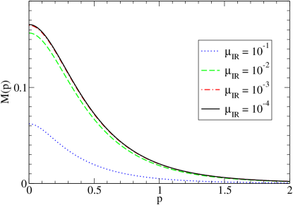
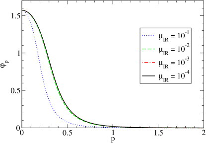
Figure 2: Mass function and chiral angle in the chiral limit for different values of the infrared regulator $\mu_{\rm IR}$. All quantities are given in appropriate units of $\sqrt{\sigma}$.

On the other hand, $A(p)$, $B(p)$ and consequently also $\omega(p)$ diverge like $\mu_{\rm IR}^{-1}$. The latter can be determined from $A(p)$ and $B(p)$ with Eq. (16) or directly by combining (11,12) to

$$\begin{array}[]{l}\omega(p)=m\sin\varphi_{p}+p\cos\varphi_{p}+\\ \displaystyle\frac{1}{2}\int\frac{d^{3}q}{(2\pi)^{3}}\;V(k)\left(\sin\varphi_{q}\sin\varphi_{p}+\hat{p}\cdot\hat{q}\cos\varphi_{q}\cos\varphi_{p}\right).\end{array}$$ (20)

The infrared divergences can be explicitly projected out by using

$$\begin{array}[]{l}\displaystyle\lim\limits_{\mu_{\rm IR}\to 0}\frac{\mu_{\rm IR}}{\pi^{2}}\int d^{3}q\;\frac{1}{(k^{2}+\mu_{\rm IR}^{2})^{2}}f(\vec{q})=\\ \displaystyle\int d^{3}q\;\delta(\vec{p}-\vec{q})f(\vec{q})=f(\vec{p}).\end{array}$$ (21)

This yields

$$A(p) = \frac{\sigma}{2\mu_{\rm IR}}\sin\varphi_{p}+A_{f}(p),$$ (22)

$$B(p) = \frac{\sigma}{2\mu_{\rm IR}}\cos\varphi_{p}+B_{f}(p),$$ (23)

$$\omega(p) = \frac{\sigma}{2\mu_{\rm IR}}+\omega_{f}(p),$$ (24)

where $A_{f}(p)$, $B_{f}(p)$, and $\omega_{f}(p)$ are infrared-finite functions.

Numerically the integration in (17) with $\mu_{\rm IR}=0$ is feasible but demanding. Alternatively one can also solve $(\ref{gapequdetaila},\ref{gapequdetailb})$ with sufficiently small but finite values for $\mu_{\rm IR}=0$. Still, in particular for very small values of $\mu_{\rm IR}$, special care has to be taken for the numerical integration in the vicinity of $\vec{q}=\vec{p}$. The convergence of $M(p)$ for $\mu_{\rm IR}\to 0$ in the chiral limit ($m=0$) has been demonstrated in Refs. Alkofer:1988tc ; AL . The mass function and the chiral angle, which are in agreement with the previous studies, are shown in the upper and lower plot of Fig. 1, respectively. The result for $\mu_{\rm IR}=10^{-4}\sqrt{\sigma}$ is already a very good approximation of the infrared limit which can be determined numerically by extrapolating the results to $\mu_{\rm IR}=0$.

An important issue is a momentum dependence of the chiral angle and dynamical mass. Their nonzero values are uniquely related in the chiral limit with the spontaneous symmetry breaking. The effect of symmetry breaking is large at low momenta and the chiral angle goes to $\pi/2$ at zero momenta. At large momenta the mass function and the chiral angle go to zero. This property is crucial for a proper understanding of chiral symmetry restoration in excited hadrons.

IV Chiral and $U(1)_{A}$ symmetry properties of the noninteracting two-quark amplitude

Given a dressed quark Green function, one can obtain a spectrum of the quark-antiquark bound states from the homogeneous Bethe-Salpeter equation in the rest frame.

Before solving the Bethe-Salpeter equation we would like to discuss a limiting case when the self-interaction is switched off, $M(p)=0$. In such a case there is no self-energy and the quark condensate is identically zero. The chiral and $U(1)_{A}$ symmetries are not broken. Then the Bethe-Salpeter amplitude is reduced to a system of massless quarks with definite chirality. In such a case properties of the system are unambiguously determined by the Poincaré invariance as well as chiral and $U(1)_{A}$ symmetries G3 . The Poincaré invariance prescribes the standard quantum numbers $J^{PC}$. The chiral and $U(1)_{A}$ properties of the system then are uniquely determined by the index of a representation of $SU(2)_{L}\times SU(2)_{R}$ that is compatible with the given $J^{PC}$ and isospin $I$. Then a complete list of states is

J = 0

$$(1/2,1/2)_{a} : 1,0^{-+}\longleftrightarrow 0,0^{++}$$

$$(1/2,1/2)_{b} : 1,0^{++}\longleftrightarrow 0,0^{-+},$$ (25)

J = 2k,   k=1,2,…

$$(0,0) : 0,J^{--}\longleftrightarrow 0,J^{++}$$

$$(1/2,1/2)_{a} : 1,J^{-+}\longleftrightarrow 0,J^{++}$$

$$(1/2,1/2)_{b} : 1,J^{++}\longleftrightarrow 0,J^{-+}$$

$$(0,1)\oplus(1,0) : 1,J^{++}\longleftrightarrow 1,J^{--}$$ (26)

J = 2k-1,   k=1,2,…

$$(0,0) : 0,J^{++}\longleftrightarrow 0,J^{--}$$

$$(1/2,1/2)_{a} : 1,J^{+-}\longleftrightarrow 0,J^{--}$$

$$(1/2,1/2)_{b} : 1,J^{--}\longleftrightarrow 0,J^{+-}$$

$$(0,1)\oplus(1,0) : 1,J^{--}\longleftrightarrow 1,J^{++}$$ (27)

The sign $\longleftrightarrow$ indicates that both given states belong to the same representation and must be degenerate. Note, that the structure of the chiral multiplets is different for mesons with different spin. In particular, for some of the $J^{PC}$ the chiral symmetry requires a doubling of states.

The $U(1)_{A}$ multiplets combine the opposite spatial parity states from the distinct $(1/2,1/2)_{a}$ and $(1/2,1/2)_{b}$ multiplets of $SU(2)_{L}\times SU(2)_{R}$.

The energy of the rotating massless quark is the same irrespective whether it is right or left, because there is no spin-orbit force in this case G2 . Then one expects a degeneracy of all chiral multiplets with the same $J$. This means that the states with the same $J$ fall into a reducible representation

$$\left[(0,1/2)\oplus(1/2,0)\right]\times\left[(0,1/2)\oplus(1/2,0)\right],$$ (28)

that combines all possible chiral representations of the quark-antiquark system with the same spin.

Certainly, once the self-energy is switched on, the chiral symmetry gets broken and there cannot be exact chiral and $U(1)_{A}$ multiplets. The effective restoration of chiral symmetry in excited hadrons is defined to occur if the following conditions are satisfied: (i) the states fall into approximate multiplets of $SU(2)_{L}\times SU(2)_{R}$ and $U(1)_{A}$ and the splittings within the multiplets ( $\Delta\mu=\mu_{+}-\mu_{-}$) vanish at $n\rightarrow\infty$ and/or $J\rightarrow\infty$ ; (ii) the splitting within the multiplet is much smaller than between the two subsequent multiplets.

To verify this prediction we have to solve the Bethe-Salpeter equation, which will be done in the following sections.

V Bethe-Salpeter equation for mesons and cancellation of the infrared divergences

The homogeneous Bethe–Salpeter equation (BSE) for a quark-antiquark bound state with total and relative four momenta $P$ and $p$, respectively, can generally be written in covariant form as

$$\chi(P,p) = -i\int\frac{d^{4}q}{(2\pi)^{4}}K(P,p,q)\;S(q+P/2)$$ (29)

$$\times \chi(P,q)S(q-P/2),$$

where $K(P,p,q)$ is called the Bethe-Salpeter kernel and $\chi(P,p)$ is the meson vertex function. In the rest frame, i.e. with the four momentum $P^{\nu}=(\mu,\vec{P}=0)$ the latter depends on the meson mass $\mu$ and all four components of $p$. Finally, for the instantaneous interaction of our model it is energy independent and BSE becomes

$$\chi(\mu,{\vec{p}}) = -i\int\frac{d^{4}q}{(2\pi)^{4}}V(|{\vec{p}}-{\vec{q}}|)\;\gamma_{0}S(q_{0}+\mu/2,{\vec{k}})$$ (30)

$$\times \chi(\mu,{\vec{q}})S(q_{0}-\mu/2,{\vec{k}})\gamma_{0}.$$

In order to solve the Bethe-Salpeter equation for mesons with the set of quantum numbers $J^{PC}$ with the given total spin $J$, parity $P$, and C-parity $C$, we expand the meson vertex function $\chi^{PC}_{JM}(\mu,{\vec{p}})$ into a set of all possible independent Poincaré-invariant amplitudes consistent with $J^{PC}$. This is done in the Appendix A. Then the Bethe-Salpeter equation transforms into a system of coupled integral equations. Such a system of equations is derived in the Appendix B. The expansion of the meson vertex functions as well as the system of coupled equations look slightly differently for three possible categories of $\bar{q}q$ mesons.

Category 1. To this category mesons with $J^{-+}$ for $J=2n$ and $J^{+-}$ for $J=2n+1$ belong. In the nonrelativistic limit these mesons have wave functions with orbital angular momentum $L=J$ and the sum of the two quark spins $S=0$.

Category 2. Mesons with $J^{++}$ for $J=2n$ and $J^{--}$ for $J=2n+1$ are in this category. In this case the nonrelativistic wave functions have $L=J\pm 1$ and $S=1$.

Category 3. This category contains mesons with $J^{--}$ for $J=2(n+1)$ and $J^{++}$ for $J=2n+1$. Their nonrelativistic wave functions have $L=J$ and $S=1$.

The relativistic quark-antiquark states with $J^{PC}=0^{--}$ do not exist in the BSE framework with an instantaneous interaction. In the nonrelativistic limit $L=0$ and $S=1$ would have to couple to $J=0$, which is impossible. The quark-antiquark states of category 4, i.e., with $J^{+-}$ for $J=2n$ and $J^{-+}$ for $J=2n+1$, do not exist in the BSE framework with the instantaneous interaction, too, as is also shown in Appendix B. There are also no corresponding nonrelativistic states. Mesons with such quantum numbers are called exotic (mesons with exotic quantum numbers) and can be realized in form of hybrids, i.e., as $q\bar{q}$ states with explicit excitation of the gluonic field, or as four-quark states. If they can also be described as quark-antiquark states in the the BSE framework with a non-instantaneous interaction is a matter of dicsussion. We do not consider them in the present paper, however.

Now we want to study the infrared limit of the Bethe-Salpeter equation and cancellation of the infrared singularities. To this end let us take a closer look at the integral equations for mesons of category 1, which are

$$\omega(p)h(p) = \frac{1}{2}\int\frac{d^{3}q}{(2\pi)^{3}}V(k)P_{J}(\hat{p}\cdot\hat{q})\left(h(q)+\frac{\mu^{2}}{4\omega(q)}g(q)\right),$$ (31a)

$$\left(\omega(p)-\frac{\mu^{2}}{4\omega(p)}\right)g(p) = h(p)$$ (31b)

$$+ \frac{1}{2}\int\frac{d^{3}q}{(2\pi)^{3}}V(k)\frac{M(p)M(q)P_{J}(\hat{p}\cdot\hat{q})+pq\left(\frac{J+1}{2J+1}P_{J+1}(\hat{p}\cdot\hat{q})+\frac{J}{2J+1}P_{J-1}(\hat{p}\cdot\hat{q})\right)}{\bar{\omega}(p)\bar{\omega}(q)}g(q).$$

Here the functions $h(p),g(p)$ are as defined in the Appendix B which along with the meson mass $\mu$ have to be found from the given equations and $\vec{k}=\vec{p}-\vec{q}$.

According to (24) and (21) there are IR divergent terms

$$\frac{\sigma}{2\mu_{\rm IR}}h(p)$$ (32)

and

$$\frac{\sigma}{2\mu_{\rm IR}}\int d^{3}q\delta(\vec{k})P_{J}(\hat{p}\cdot\hat{q})h(q)=\frac{\sigma}{2\mu_{\rm IR}}h(p)$$ (33)

on the left and right hand sides of (31a), respectively. The term with $g(q)$ in the integrand of (31a) comes with a factor $1/\omega(q)={\cal O}(\mu_{\rm IR})$ and the integral over this term becomes the IR finite expression

$$\frac{\mu^{2}}{4}g(p).$$ (34)

Similarly there are IR divergent terms

$$\frac{\sigma}{2\mu_{\rm IR}}g(p)$$ (35)

and

$$\frac{\sigma}{2\mu_{\rm IR}}\int d^{3}q\delta(\vec{k})\frac{M(p)M(q)P_{J}(\hat{p}\cdot\hat{q})+pq\left(\frac{J+1}{2J+1}P_{J+1}(\hat{p}\cdot\hat{q})+\frac{J}{2J+1}P_{J-1}(\hat{p}\cdot\hat{q})\right)}{\bar{\omega}(p)\bar{\omega}(q)}g(q)=\frac{\sigma}{2\mu_{\rm IR}}g(p)$$ (36)

on the left and right hand sides of (31b), respectively. The second term in the bracket on the left hand side has a factor $\omega(p)^{-1}={\cal{O}}(\mu_{\rm IR})$ which vanishes in the IR limit. On the right hand side there is an IR finite term $h(p)$. One sees that the IR divergent terms on both sides of both equations cancel and we end up with the coupled system of integral equations

$$\omega_{f}(p)h(p) = \frac{\mu^{2}}{4}g(p)+\frac{1}{2}\int\frac{d^{3}q}{(2\pi)^{3}}V_{f}(k)P_{J}(\hat{p}\cdot\hat{q})h(q),$$ (37a)

$$\omega_{f}(p)g(p) = h(p)$$ (37b)

$$+ \frac{1}{2}\int\frac{d^{3}q}{(2\pi)^{3}}V_{f}(k)\frac{M(p)M(q)P_{J}(\hat{p}\cdot\hat{q})+pq\left(\frac{J+1}{2J+1}P_{J+1}(\hat{p}\cdot\hat{q})+\frac{J}{2J+1}P_{J-1}(\hat{p}\cdot\hat{q})\right)}{\bar{\omega}(p)\bar{\omega}(q)}g(q),$$

with

$$V_{f}(k)=V(k)-\frac{\sigma}{\mu_{\rm IR}}(2\pi)^{3}\delta(\vec{k}),$$ (38)

which has a finite IR limit.

In an analogous manner all IR divergences from the integral equations for the mesons of category 2 and 3 can be removed. The IR finite integral equations for mesons in category 2 are

$$\displaystyle\omega_{f}(p)h_{1}(p) = \displaystyle\frac{\mu^{2}}{4}g_{1}(p)+\frac{1}{2}\int\frac{d^{3}q}{(2\pi)^{3}}V_{f}(k)\left\{\left(\frac{J}{2J+1}P_{J+1}(\hat{p}\cdot\hat{q})+\frac{J+1}{2J+1}P_{J-1}(\hat{p}\cdot\hat{q})\right)h_{1}(q)\right.$$ (39a)

$$\displaystyle+\left.\frac{M(q)}{\bar{\omega}(q)}\frac{\sqrt{J(J+1)}}{2J+1}\left(P_{J+1}(\hat{p}\cdot\hat{q})-P_{J-1}(\hat{p}\cdot\hat{q})\right)h_{2}(q)\right\},$$

$$\displaystyle\omega_{f}(p)g_{1}(p) = h_{1}(p)+\displaystyle\frac{1}{2}\int\frac{d^{3}q}{(2\pi)^{3}}V_{f}(k)\left\{\frac{pqP_{J}(\hat{p}\cdot\hat{q})+M(p)M(q)\left(\frac{J}{2J+1}P_{J+1}(\hat{p}\cdot\hat{q})+\frac{J+1}{2J+1}P_{J-1}(\hat{p}\cdot\hat{q})\right)}{\bar{\omega}(p)\bar{\omega}(q)}g_{1}(q)\right.$$ (39b)

$$\displaystyle+\left.\frac{M(p)}{\bar{\omega}(p)}\frac{\sqrt{J(J+1)}}{2J+1}\left(P_{J+1}(\hat{p}\cdot\hat{q})-P_{J-1}(\hat{p}\cdot\hat{q})\right)g_{2}(q)\right\}$$

$$\displaystyle\omega_{f}(p)h_{2}(p) = \displaystyle\frac{\mu^{2}}{4}g_{2}(p)+\frac{1}{2}\int\frac{d^{3}q}{(2\pi)^{3}}V_{f}(k)\left\{\frac{pqP_{J}(\hat{p}\cdot\hat{q})+M(p)M(q)\left(\frac{J+1}{2J+1}P_{J+1}(\hat{p}\cdot\hat{q})+\frac{J}{2J+1}P_{J-1}(\hat{p}\cdot\hat{q})\right)}{\bar{\omega}(p)\bar{\omega}(q)}\right.h_{2}(q)$$ (39c)

$$\displaystyle+\left.\frac{M(p)}{\bar{\omega}(p)}\frac{\sqrt{J(J+1)}}{2J+1}\left(P_{J+1}(\hat{p}\cdot\hat{q})-P_{J-1}(\hat{p}\cdot\hat{q})\right)h_{1}(q)\right\},$$

$$\displaystyle\omega_{f}(p)g_{2}(p) = h_{2}(p)+\displaystyle\frac{1}{2}\int\frac{d^{3}q}{(2\pi)^{3}}V_{f}(k)\left\{\left(\frac{J+1}{2J+1}P_{J+1}(\hat{p}\cdot\hat{q})+\frac{J}{2J+1}P_{J-1}(\hat{p}\cdot\hat{q})\right)g_{2}(q)\right.$$ (39d)

$$\displaystyle+\left.\frac{M(q)}{\bar{\omega}(q)}\frac{\sqrt{J(J+1)}}{2J+1}\left(P_{J+1}(\hat{p}\cdot\hat{q})-P_{J-1}(\hat{p}\cdot\hat{q})\right)g_{1}(q)\right\}.$$

Note that the number of the auxiliary functions $h_{1},g_{1},h_{2},g_{2}$ as well as the number of coupled equations in the present case is twice larger than for mesons of category 1. This is related to the number of independent components in $\chi^{PC}_{JM}(\mu,\vec{p})$ for $J>0$. However, for the states $0^{++}$ within the same category only the last two equations (39c) - (39d) apply, because in this case there are only two independent functions $h_{2},g_{2}$.

For mesons in category 3 we have:

$$\omega_{f}(p)h(p) = \frac{\mu^{2}}{4}g(p)$$ (40a)

$$+ \displaystyle\frac{1}{2}\int\frac{d^{3}q}{(2\pi)^{3}}V_{f}(k)\frac{M(p)M(q)P_{J}(\hat{p}\cdot\hat{q})+pq\left(\frac{J}{2J+1}P_{J+1}(\hat{p}\cdot\hat{q})+\frac{J+1}{2J+1}P_{J-1}(\hat{p}\cdot\hat{q})\right)}{\bar{\omega}(p)\bar{\omega}(q)}h(q),$$

$$\omega_{f}(p)g(p) = h(p)+\frac{1}{2}\int\frac{d^{3}q}{(2\pi)^{3}}V_{f}(k)P_{J}(\hat{p}\cdot\hat{q})g(q).$$ (40b)

From the integral equations the normalization of the vertex functions cannot be determined. One can derive a normalization condition by demanding that the charge of the isovector mesons with isospin projection $+1$ must be one, or equivalently by normalizing the wave function by

$$\rm{tr}\int\frac{d^{3}p}{(2\pi)^{3}} \!\!\!\!\!\!\left(\psi_{+JM}^{PC}{}^{\dagger}(\mu,\vec{p})\psi_{+JM}^{PC}(\mu,\vec{p})\right.$$ (41)

$$\!\!\!\!\!\!\!\!\!-\left.\psi_{-JM}^{PC}{}^{\dagger}(\mu,\vec{p})\psi_{-JM}^{PC}(\mu,\vec{p})\right)=2\mu$$

(see the Appendix C for the definition of the wave function), where traces in Dirac space and color space have to be taken, the latter giving just a factor 3. Then for mesons of categories 1 and 3 this yields

$$\frac{3}{4\pi}\int\frac{d^{3}p}{(2\pi)^{3}}h(p)g(p)=1.$$ (42)

For mesons of category 2 the normalization condition becomes

$$\frac{3}{4\pi}\sum\limits_{i=1}^{2}\int\frac{d^{3}p}{(2\pi)^{3}}h_{i}(p)g_{i}(p)={\cal N}_{1}+{\cal N}_{2}=1,$$ (43)

Here ${\cal N}_{1}$ and ${\cal N}_{2}$ represent the normalization factors of two coupled amplitudes, $(h_{1},g_{1})$ and $(h_{2},g_{2})$. Since these amplitudes are mixed by the dynamical mass of quarks, $M(p)$, a mixing angle $\alpha_{M}$ can be defined by ${\cal N}_{1}=\sin^{2}\alpha_{M}$ and ${\cal N}_{2}=\cos^{2}\alpha_{M}$. Obviously in the limit $M(p)\rightarrow 0$ the mixing vanishes.

VI Effective restoration of chiral symmetry for mesons

In this section we demonstrate that in the limit of the vanishing dynamical mass $M(p)\rightarrow 0$ the Bethe-Salpeter equation of the previous section recovers all the anticipated chiral multiplets (25)-(27).

For $M(p)=0$ the integral equations (37), which describe mesons of category 1, i.e. , with $J^{-+}$ for $J=2n$ and $J^{+-}$ for $J=2n+1$, become

$$\omega_{f}(p)h(p)=\frac{\mu^{2}}{4}g(p)+\frac{1}{2}\int\frac{d^{3}q}{(2\pi)^{3}}V_{f}(k)P_{J}(\hat{p}\cdot\hat{q})h(q),$$ (44a)

$$\omega_{f}(p)g(p)=h(p)+\frac{1}{2}\int\frac{d^{3}q}{(2\pi)^{3}}V_{f}(k)\frac{(J+1)P_{J+1}(\hat{p}\cdot\hat{q})+JP_{J-1}(\hat{p}\cdot\hat{q})}{2J+1}g(q).$$ (44b)

For mesons of category 2, i.e., with $J^{++}$ for $J=2n$ ($J\neq 0$) and $J^{--}$ for $J=2n+1$, the four coupled integral equations (39) decouple into two independent systems of equations

$$\omega_{f}(p)h_{1}(p)=\frac{\mu^{2}}{4}g_{1}(p)+\frac{1}{2}\int\frac{d^{3}q}{(2\pi)^{3}}V_{f}(k)\frac{JP_{J+1}(\hat{p}\cdot\hat{q})+(J+1)P_{J-1}(\hat{p}\cdot\hat{q})}{2J+1}h_{1}(q),$$ (45a)

$$\omega_{f}(p)g_{1}(p)=h_{1}(p)+\frac{1}{2}\int\frac{d^{3}q}{(2\pi)^{3}}V_{f}(k)P_{J}(\hat{p}\cdot\hat{q})g_{1}(q)$$ (45b)

and

$$\omega_{f}(p)h_{2}(p)=\frac{\mu^{2}}{4}g_{2}(p)+\frac{1}{2}\int\frac{d^{3}q}{(2\pi)^{3}}V_{f}(k)P_{J}(\hat{p}\cdot\hat{q})h_{2}(q),$$ (45c)

$$\omega_{f}(p)g_{2}(p)=h_{2}(p)+\frac{1}{2}\int\frac{d^{3}q}{(2\pi)^{3}}V_{f}(k)\frac{(J+1)P_{J+1}(\hat{p}\cdot\hat{q})+JP_{J-1}(\hat{p}\cdot\hat{q})}{2J+1}g_{2}(q).$$ (45d)

For the $0^{++}$ states within this category only equations (45c)-(45d) apply.

For the mesons of category 3, i.e., with $J^{++}$ for $J=2n+1$ and $J^{--}$ for $J=2(n+1)$, the Bethe-Salpeter equation takes the form

$$\omega_{f}(p)h(p)=\frac{\mu^{2}}{4}g(p)+\frac{1}{2}\int\frac{d^{3}q}{(2\pi)^{3}}V_{f}(k)\frac{JP_{J+1}(\hat{p}\cdot\hat{q})+(J+1)P_{J-1}(\hat{p}\cdot\hat{q})}{2J+1}h(q),$$ (46a)

$$\omega_{f}(p)g(p)=h(p)+\frac{1}{2}\int\frac{d^{3}q}{(2\pi)^{3}}V(k)P_{J}(\hat{p}\cdot\hat{q})g(q).$$ (46b)

We see that the equations (44a) - (44b) become identical to the equations (45c) - (45d) as well as the equations (45a) - (45b) are identical to equations (46a) - (46b). Note, that there is no isospin dependence of the interaction, i.e. each system of coupled equations describes both I=0 and I=1 states which are exactly degenerate. Then we recover that the equations above fall into chiral multiplets (25)-(27) and both $SU(2)_{L}\times SU(2)_{R}$ and $U(1)_{A}$ are manifest. Hence if the typical momentum of quarks is large, as it is anticipated in the highly-excited mesons, the spectrum should be organized into chiral and $U(1)_{A}$ multiplets , because at large momenta dynamical mass of quarks $M(p)$ vanishes.

VII Numerical results for spectrum

The method of solution for the BSE used in this work is described in Appendix D. In Table 1 we present our results for the spectrum for the two-flavor ($u$ and $d$) mesons in the chiral limit $m=0$. Due to chiral symmetry breaking there is a mixing between $(h_{1},g_{1})$ and $(h_{2},g_{2})$ amplitudes for mesons of category 2 (but not for the $0^{++}$ states). In the language of chiral representations this mixing means that for mesons of category 2 with $J=2n+1$ the representations $(0,0)$ and $(1/2,1/2)_{a}$ are mixed in the mesons $0,J^{--}$ as well as the representations $(0,1)\oplus(1,0)$ and $(1/2,1/2)_{b}$ are mixed in the mesons $1,J^{--}$. For mesons of category 2 with $J=2n,J>0$ the representations $(0,0)$ and $(1/2,1/2)_{a}$ are mixed in the $0,J^{++}$ states and the representations $(0,1)\oplus(1,0)$ and $(1/2,1/2)_{b}$ are mixed in the mesons $1,J^{++}$. The mesons of the category 2 in the Table are assigned to a definite chiral representation according to the chiral Bethe-Salpeter amplitude which dominates in the meson wave function, which is determined by the relative magnitude of the normalization factors ${\cal N}_{1}$ and ${\cal N}_{2}$ in (43).

Note that within the present model there are no vacuum fermion loops. Then since the interaction between quarks is isospin-independent the states with the same $J^{PC}$ but different isospins from the distinct multiplets $(1/2,1/2)_{a}$ and $(1/2,1/2)_{b}$ as well as the states with the same $J^{PC}$ but different isospins from $(0,0)$ and $(0,1)\oplus(1,0)$ representations are exactly degenerate. Hence it is enough to show a complete set of the isovector (or isoscalar) states.

The presented results are accurate within the quoted digits at least for states with small $J$ and for states with higher $J$ but small $n$. At larger $J$ for larger $n$ numerical errors accumulate in the second digit after comma.

The axial anomaly is absent within the present model, because there are no vacuum fermion loops here. Even so there are no exact $U(1)_{A}$ multiplets, because this symmetry is broken also by the quark condensate of the vacuum. The mechanism of the $U(1)_{A}$ breaking and restoration is exactly the same as for $SU(2)_{L}\times SU(2)_{R}$.

The excited mesons fall into approximate chiral and $U(1)_{A}$ multiplets and all conditions of the effective symmetry restorations are satisfied. We observe a very fast restoration of both $SU(2)_{L}\times SU(2)_{R}$ and $U(1)_{A}$ symmetries with increasing $J$ and essentially more slow restoration with increasing of $n$.

Table 1: Masses of isovector mesons in units of $\sqrt{\sigma}$.

chiral	$J^{PC}$	radial excitation $n$
multiplet		0	1	2	3	4	5	6
$(1/2,1/2)_{a}$	$0^{-+}$	0.00	2.93	4.35	5.49	6.46	7.31	8.09
$(1/2,1/2)_{b}$	$0^{++}$	1.49	3.38	4.72	5.80	6.74	7.57	8.33
$(1/2,1/2)_{a}$	$1^{+-}$	2.68	4.03	5.16	6.14	7.01	7.80	8.53
$(1/2,1/2)_{b}$	$1^{--}$	2.78	4.18	5.32	6.30	7.17	7.96	8.68
$(0,1)\oplus(1,0)$	$1^{--}$	1.55	3.28	4.56	5.64	6.57	7.40	8.16
$(0,1)\oplus(1,0)$	$1^{++}$	2.20	3.73	4.95	5.98	6.88	7.69	8.43
$(1/2,1/2)_{a}$	$2^{-+}$	3.89	4.98	5.94	6.80	7.59	8.31	8.99
$(1/2,1/2)_{b}$	$2^{++}$	3.91	5.02	6.00	6.88	7.67	8.40	9.09
$(0,1)\oplus(1,0)$	$2^{++}$	3.60	4.67	5.64	6.51	7.32	8.06	8.75
$(0,1)\oplus(1,0)$	$2^{--}$	3.67	4.80	5.80	6.68	7.49	8.23	8.91
$(1/2,1/2)_{a}$	$3^{+-}$	4.82	5.77	6.62	7.41	8.13	8.81	9.45
$(1/2,1/2)_{b}$	$3^{--}$	4.82	5.78	6.65	7.44	8.17	8.86	9.50
$(0,1)\oplus(1,0)$	$3^{--}$	4.68	5.63	6.48	7.26	7.99	8.67	9.30
$(0,1)\oplus(1,0)$	$3^{++}$	4.69	5.66	6.53	7.32	8.06	8.74	9.39
$(1/2,1/2)_{a}$	$4^{-+}$	5.59	6.45	7.23	7.96	8.64	9.28	9.89
$(1/2,1/2)_{b}$	$4^{++}$	5.59	6.45	7.24	7.97	8.66	9.30	9.91
$(0,1)\oplus(1,0)$	$4^{++}$	5.51	6.36	7.15	7.88	8.56	9.19	9.80
$(0,1)\oplus(1,0)$	$4^{--}$	5.51	6.37	7.16	7.90	8.58	9.23	9.84
$(1/2,1/2)_{a}$	$5^{+-}$	6.27	7.05	7.78	8.47	9.11	9.72	10.3
$(1/2,1/2)_{b}$	$5^{--}$	6.27	7.06	7.79	8.47	9.12	9.73	10.3
$(0,1)\oplus(1,0)$	$5^{--}$	6.21	7.00	7.73	8.41	9.06	9.67	10.2
$(0,1)\oplus(1,0)$	$5^{++}$	6.21	7.00	7.73	8.42	9.07	9.68	10.3
$(1/2,1/2)_{a}$	$6^{-+}$	6.88	7.61	8.29	8.94	9.55	10.1	10.7
$(1/2,1/2)_{b}$	$6^{++}$	6.88	7.61	8.29	8.94	9.56	10.1	10.7
$(0,1)\oplus(1,0)$	$6^{++}$	6.83	7.57	8.25	8.90	9.51	10.1	10.7
$(0,1)\oplus(1,0)$	$6^{--}$	6.83	7.57	8.26	8.90	9.52	10.1	10.7

The spectrum of the $J=0,1,2$ mesons is shown in Figs. 3 - 5.

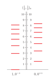
Figure 3: Spectra of $J=0$ mesons (masses in units of $\sqrt{\sigma}$).

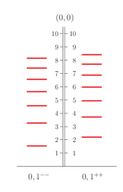
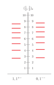
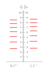
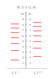
Figure 4: Spectra of $J=1$ mesons (masses in units of $\sqrt{\sigma}$).

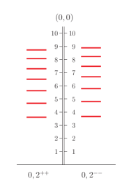
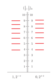
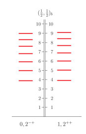
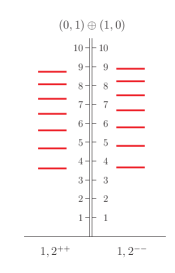
Figure 5: Spectra of $J=2$ mesons (masses in units of $\sqrt{\sigma}$).

In Fig. 6 the rates of the symmetry restoration against the radial quantum number $n$ and spin $J$ are shown. It is seen that with the fixed $J$ the splitting within the multiplets $\Delta M$ decreases asymptotically as $1/\sqrt{n}$, dictated by the asymptotic linearity of the radial Regge trajectories with different intercepts. With the fixed $n$ the $J$-rate of the symmetry restoration is much faster.

In the limit $n\rightarrow\infty$ or $J\rightarrow\infty$ one observes a complete degeneracy of all multiplets, which means that the states fall into representation (28) that combines all possible chiral representations for the systems of two massless quarks G3 . This means that in this limit the loop effects disappear completely and the system becomes classical G5 ; G6 . The analytical proof for this larger degeneracy will be given in the next section.

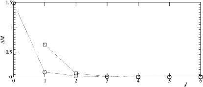
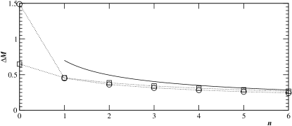
Figure 6: Mass splittings in units of $\sqrt{\sigma}$ for isovector mesons of the chiral multiplets $(1/2,1/2)_{a}$ and $(1/2,1/2)_{b}$ (circles) and within the multiplet $(0,1)\oplus(1,0)$ (squares) against $J$ for $n=0$ (top) and against $n$ for $J=0$ and $J=1$, respectively (bottom). The full line in the bottom plot is $0.7\sqrt{\sigma/n}$.

In Fig. 7 the angular and radial Regge trajectories are shown. Both kinds of trajectories exhibit asymptotically linear behavior. This has to be expected a-priory, because at large $J$ or $n$ all higher Fock components are suppressed and asymptotically vanish (it will be later well seen from the meson wave functions).Then the semiclassical description of the states with large $n$ or $J$ with the linear potential requires the linear Regge trajectories, see, e.g., ref. semicl . There are deviations from the linear behavior at finite $J$ and $n$, however. This fact is obviously related to the chiral symmetry breaking effects for lower mesons. Note, that the chiral symmetry requires a doubling of some of the radial and angular Regge trajectories for $J=1,2,..$. This is a highly nontrivial prediction of chiral symmetry. For example, some of the rho-mesons lie on the trajectory that is characterized by the chiral index (0,1)+(1,0), while the other fit the trajectory with the chiral index $(1/2,1/2)_{b}$.

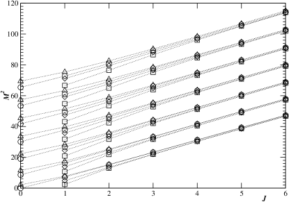
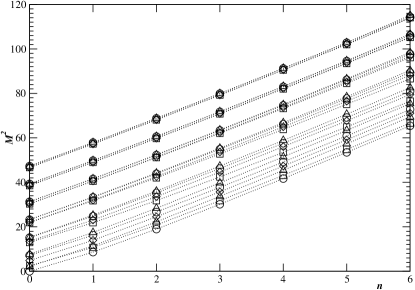
Figure 7: Angular (top) and radial (bottom) Regge trajectories for isovector mesons with $M^{2}$ in units of $\sigma$. Mesons of the chiral multiplet $(1/2,1/2)_{a}$ are indicated by circles, of $(1/2,1/2)_{b}$ by triangles, and of $(0,1)\oplus(1,0)$ by squares ($J^{++}$ and $J^{--}$ for even and odd $J$, respectively) and diamonds ($J^{--}$ and $J^{++}$ for even and odd $J$, respectively).

The numerical result for the quark condensate is $\langle\bar{q}q\rangle=(-0.231\sqrt{\sigma})^{3}$, which agrees with the previous studies within the same model. If we fix the string tension from the phenomenological angular Regge trajectories, then $\sqrt{\sigma}\approx 300$ – $400$ MeV and hence the quark condensate is between $(-70\ \mbox{MeV})^{3}$ and $(-90\ \mbox{MeV})^{3}$ which obviously underestimates the phenomenological value. Probably this indicates that other gluonic interactions could also contribute to chiral symmetry breaking.

VIII Higher representations for excited states

We have mentioned in the previous section that an approximate degeneracy within the higher representation (28) is observed for highly excited mesons. Below we demonstrate this property analytically.

Let us compare the integral equations (37) and (40) for mesons of categories 1 and 3, respectively. By exchanging $h$ and $\frac{\mu}{2}g$ for the latter (40b) becomes (37a) and the difference between (37b) and (40a) reduces to different coefficients in front of the Legendre polynomials, i.e. one has

$$\frac{(J+1)P_{J+1}(\hat{p}\cdot\hat{q})+JP_{J-1}(\hat{p}\cdot\hat{q})}{2J+1}$$ (47)

and

$$\frac{JP_{J+1}(\hat{p}\cdot\hat{q})+(J+1)P_{J-1}(\hat{p}\cdot\hat{q})}{2J+1},$$ (48)

respectively. The same factors are also seen in eqs. (44a)-(46b). The difference between (47) and (48) vanishes for large $J$. This means that for large $J$ there appears degeneracy within the whole reducible chiral multiplet $[(0,1/2)\oplus(1/2,0)]\times[(0,1/2)\oplus(1/2,0)]$ which combines all possible chiral representations of the quark-antiquark systems with the same $J$.

Will we see similar higher degree of degeneracy at large radial quantum number $n$ but finite $J$? The answer is yes, which is demonstrated in what follows.

In general, for a large meson mass, i.e. $n$ and/or $J$ large, the quark-antiquark component $\psi_{+}$ of the meson wave function propagating forward in time be dominant against the backward-propagating component $\psi_{-}$ (see Appendix C). In the IR limit $\mu/\omega(p)$ in (110)–(113) goes to zero, which means that for all three categories of mesons $\psi_{+}\sim 1/2(h+\frac{\mu}{2}g)$ and $\psi_{-}\sim 1/2(h-\frac{\mu}{2}g)$. For highly excited mesons, by neglecting the latter and setting

$$\psi_{+}\approx h\approx\frac{\mu}{2}g,$$ (49)

one ends up with only one equation for $\psi_{+}$ for all quark-antiquark states with the given $J$ and $n$, i.e.,

$$\omega_{f}(p)\psi_{+}(p) = \frac{\mu}{2}\psi_{+}(p)$$ (50)

$$+ \frac{1}{2}\int\frac{d^{3}q}{(2\pi)^{3}}V_{f}(k)P_{J}(\hat{p}\cdot\hat{q})\psi_{+}(q).$$

Hence all possible states with the same $J$ at the given large $n$ fall into the $[(0,1/2)\oplus(1/2,0)]\times[(0,1/2)\oplus(1/2,0)]$ representation and the degeneracy becomes exact when $J$ and/or $n$ approach infinity.

IX Wave functions

At large $J$ or $n$ the semiclassical description requires that the higher quark Fock components be suppressed relative the leading one and asymptotically vanish. This is because the higher Fock components manifestly represent effects of quantum fluctuations. The leading Fock component is the forward-propagating quark-antiquark component $\psi_{+}(p)$, defined in the Appendix C, while the higher Fock components contain necessarily the backward-propagating quark-antiquark states $\psi_{-}(p)$. In Figs. 8 and 9 we show that for mesons of category 1 with large radial quantum number $n$ and/or spin $J$ the forward-propagating component $\psi_{+}(p)$ becomes indeed much larger than the backward-propagating component $\psi_{-}(p)$.

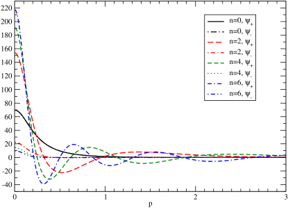
Figure 8: Components $\psi_{+}(p)$ and $\psi_{-}(p)$ of the wave functions for ground and radially excited states for mesons $0^{-+}$ of category 1. All quantities are given in appropriate units of $\sqrt{\sigma}$. Notice that the ground state (Goldstone boson) has $\mu=0$ and thus $\psi_{-}(p)=\psi_{+}(p)$, hence the two curves for $n=0$ coincide.

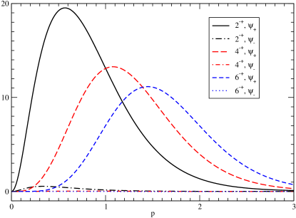
Figure 9: Components $\psi_{+}(p)$ and $\psi_{-}(p)$ of the wave functions for mesons $J^{-+}$ of category 1 with radial quantum number $n=0$ and spin $J=2,4,6$. All quantities are given in appropriate units of $\sqrt{\sigma}$.

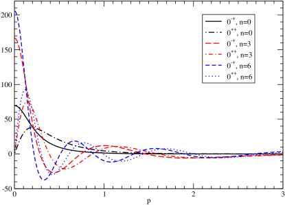
Figure 10: Components $\psi_{+}(p)$ of ground states and radial excitations of pseudoscalar and scalar mesons. All quantities are given in appropriate units of $\sqrt{\sigma}$.

The wave functions of mesons of categories 2 and 3 behave similarly. In order to study the behavior of the wave functions of mesons with large $n$ and/or $J$ we can thus restrict ourselves to $\psi_{+}(p)$.

In Fig. 10 we compare the wave functions of chiral partners in $(1/2,1/2)$ representations for mesons with $0^{-+}$ and $0^{++}$, for the ground states ($n=0$) and radial excitations $n=3,6$. A principal difference between pseudoscalar and scalar mesons is the behavior of the wave functions for momentum $p\to 0$ which go to a constant for the former and to zero like $p$ for the latter. Thus at small $p$ there is a large difference between the wave functions of pseudoscalar and scalar mesons with the same radial quantum number $n$ even if $n$ is large. At large $p$ (where dynamical mass becomes small and effective restoration of chiral symmetry takes place) the wave functions of the radially excited pseudoscalar and scalar mesons behave similar but there is a shift in the positions of nodes and maxima/minima. This persisting difference of the wave functions is a reason for a slow rate of chiral restoration in meson masses with increasing $n$.

For $J>0$ there are four different mesons with the given isospin at fixed $n$ and $J$. One of category 1 and 3, respectively, and two of category 2.

Consider mesons of category 2. They are mixings of two different chiral representations with radial functions $\psi_{1+}(p)$ and $\psi_{2+}(p)$, respectively. The mixing is characterized by the size of the normalization factors ${\cal N}_{1}$ and ${\cal N}_{2}=1-{\cal N}_{1}$.

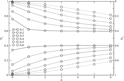
Figure 11: ${\cal N}_{1}$ (or ${\cal N}_{2}=1-{\cal N}_{1})$ for mesons of category 2. For each $J>0$ and $n$ there is one state with ${\cal N}_{1}>{\cal N}_{2}=1-{\cal N}_{1}$ and vice versa.

In Fig. 11 we show ${\cal N}_{1}$ $({\cal N}_{2})$ for all states of category 2 considered in this work. For given $n$ the mixing decreases with increasing $J$. At large $J$ there is one almost unmixed state with ${\cal N}_{1}\approx 1$ and one almost unmixed state with ${\cal N}_{2}\approx 1$. The former belongs to the chiral multiplet $(0,0)$ and $(0,1)\oplus(1,0)$ in case of isospin $0$ and $1$, respectively and the latter to $(\frac{1}{2},\frac{1}{2})_{a}$ and $(\frac{1}{2},\frac{1}{2})_{b}$ in case of isospin $0$ and $1$, respectively. In contrast, for given $J$ the mixing first increases with increasing $n$ and then saturates. The saturation value seems to be of about 0.6 for $J=1$. For larger $J$ such a saturation is not yet reached for $n=6$.

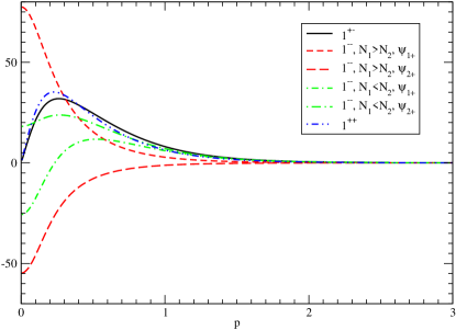
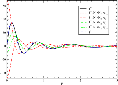
Figure 12: Components $\psi_{+}(p)$ of mesons with $J=1$. Upper plot: $n=0$, lower plot: $n=6$. All quantities are given in appropriate units of $\sqrt{\sigma}$.

In Fig. 12 we show the wave functions For $J=1$ and $n=0$ and $n=6$. In both cases the wave functions of mesons of category 1 and 3 are rather similar to each other. These wave functions go to zero for $p\to 0$ contrary to the wave functions of the mesons of category 2 which go to a constant. At small momenta the coupling between $\psi_{1}(p)$ and $\psi_{2}(p)$ in mesons of category 2 becomes large and thus there is a rather strong mixing even for high radial excitations.

The radial wave functions of states with $n=0$ and increasing $J$ are shown in Fig. 13 for $J=2,4,6$. Already for $J=2$ four of these functions look rather similar. These are the ones for the mesons of category 1 and 3 and in each case the larger function of the two mesons of category 2, which is in the first case $\psi_{1+}(p)$ and in the second case $\psi_{2+}(p)$. The two other functions ($\psi_{2+}(p)$ and $\psi_{1+}(p)$ in the first and second case, respectively) are smaller. From Fig. 11 one sees that ${\cal N}_{1}$ (or ${\cal N}_{2}$) are both larger than $0.8$ in the first and second case, respectively. For $J=4$ and even more for $J=6$ the mixing becomes very small and consequently the physics is determined by the four almost indistinguishable radial functions. Consequently there appears approximate degeneracy of all mesons for given $n$ at large $J$. This is in accord with the discussion in the preceeding section. Obviously the wave function for larger $J$ are strongly suppressed at small momenta, i.e., the radial function goes to zero as $p^{J}$ for mesons of categories 1 and 3 and as $p^{J-1}$ for mesons of category 2. It is this feature which explains a fast chiral restoration with increasing $J$, because the chiral symmetry breaking dynamical mass $M(p)$ is essential only at small momenta.

For higher radial excitations the wave functions acquire nodes and the first bump is shifted towards lower momenta as we show in Fig. 14 for $J=6$ and $n=6$. That explains why at given $J$ for increasing $n$ the mixing becomes larger.

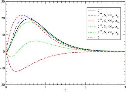
Figure 13: Components $\psi_{+}(p)$ of mesons with $J=2,4,6$ and $n=0$. All quantities are given in appropriate units of $\sqrt{\sigma}$.

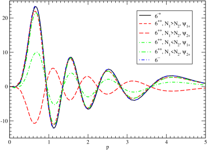
Figure 14: Components $\psi_{+}(p)$ of mesons with $J=6$ and $n=6$. All quantities are given in appropriate units of $\sqrt{\sigma}$.

X Conclusions

In this paper we have demonstrated explicitly a fast effective chiral symmetry restoration in excited mesons with increasing $J$ and a slow restoration with increasing $n$. To this end we used a model where the only interaction between quarks is linear instantaneous Coulomb-like confining interaction between color charges. This model contains all the necessary ingredients - it is confining and manifestly chirally symmetric. Chiral symmetry breaking is provided in the standard way through the nonperturbative self interactions of quarks while the meson spectrum is obtained from the Bethe-Salpeter equation.

The key implication of dynamical chiral symmetry breaking is that the quarks acquire the dynamical Lorentz-scalar mass which is exclusively of quantum (loop) origin. This dynamical mass is strongly momentum-dependent and vanishes fast at larger momenta. In highly excited states the quantum (loop) effects must be suppressed relative the classical contributions and the spectrum exhibits an approximate $SU(2)_{L}\times SU(2)_{R}$ and $U(1)_{A}$ symmetry. Microscopically this is because a typical momentum of valence quarks increases higher in the spectrum and consequently their dynamical Lorentz-scalar mass, which violates chiral symmetry, becomes small and asymptotically vanishes.

Within nonrelativistic or semirelativistic quark models the effective chiral restoration cannot be reproduced as a matter of principle, because (i) the constituent mass of quarks is an input parameter and is momentum-independent, (ii) the notion of the quark chirality is absent within a nonrelativistic or semirelativistic approach, (iii) a Lorentz-scalar confining interaction, which is typically assumed in these quark models, breaks chiral symmetry manifestly.

We have demonstrated explicitly that in the high-lying mesons all higher Fock components are strongly suppressed relative the leading $\bar{q}q$ one and a very fast restoration of chiral symmetry happens with increasing $J$ and rather slow one with increasing $n$. A reason for the former is that with larger $J$ the radial wave function vanishes at small relative momenta, and hence the large chiral-symmetry breaking dynamical mass becomes irrelevant. The slower rate of the restoration in the latter case is due to the fact that at $J=0$ the wave function at small momenta does not vanish for pseudoscalar mesons, so that even though a typical momentum of quarks increases with $n$, the small momentum dynamical mass of quarks always contributes to some extent.

All possible states for a given $n$ and large $J$ fall into higher representations $[(0,1/2)\oplus(1/2,0)]\times[(0,1/2)\oplus(1/2,0)]$ that combine all possible chiral multiplets with the given $J$ and $n$. The same property is observed for large $n$ at a given $J$, though a degree of degeneracy is smaller. This property means that in both these cases the quantum loop effects become irrelevant and all possible states with different orientations of quark chirality become equivalent.

We have shown that both radial and angular Regge trajectories are linear asymptotically. At smaller $J$ and/or $n$ the linear form is broken due to chiral symmetry breaking effects. Each Regge trajectory is characterized by the proper chiral index and hence the amount of independent Regge trajectories coincides with the amount of chiral representations. Consequently for many mesons there are two independent Regge trajectories at given $I,J^{PC}$, because in the chirally restored regime there are two independent and degenerate states with the same $I,J^{PC}$ which belong to different chiral representations.

XI Acknowledgments

RFW acknowledges helpful discussions with R. Alkofer, M. Kloker, and A. Krassnigg. This work was supported by the Austrian Science Fund (projects P16310-N08 and P19168-N16) and by DFG (project Al 279/5-1).

XII Appendix A

In this Appendix we discuss a general parametrization of the vertex function and its specific form for mesons of all categories with the instantaneous interaction.

For a meson with mass $\mu$, spin $J$, intrinsic parity $P$ and $C$-parity $C$ the vertex function $\chi^{PC}_{JM}(P,p)$ can be written as a sum of eight (four for $J=0$) components, where $M=-J,\ldots,J$ is the $z$-projection of $J$ in the rest frame of the meson. $P^{\nu}$ and $p^{\nu}$ are the total and relative four-momenta of the quark-antiquark system, respectively. Each component contains a function $\tilde{\chi}_{i}$ which depends on the two invariants $p^{2}$ and $(p.P)^{2}$ (notice that $p.P$ is Lorentz-invariant but changes its sign under the $C$-parity transformation). Since we are only interested in spectra in this paper we can restrict ourselves to the rest frame of the meson (i.e., the frame with $P^{\nu}=(\mu,0,0,0)$), where the vertex function depends on $\mu$, $p_{0}$ and $\vec{p}$ and each component contains a function $\chi_{i}$ of the two variables $p_{0}^{2}$ and $|\vec{p}|$. Some of the components contain a factor $p_{0}$ and are thus odd functions of $p_{0}$. At the same time, for an instantaneous interaction the vertex function in the rest frame is independent of $p_{0}$. Thus all components which are odd in $p_{0}$ must vanish. The function $\chi_{i}$ of the remaining components depend only on $p=|\vec{p}|$. Depending on the quantum numbers $J^{PC}$ there are four different categories of mesons. In the following we give the general expressions for the vertex function $\chi^{PC}_{JM}(P,p)$ in a general frame, $\chi^{PC}_{JM}(\mu,p_{0},\vec{p})$ in the rest frame and $\chi^{PC}_{JM}(\mu,\vec{p})$ in the rest frame and an instantaneous interaction.

Category 1: Mesons with $J^{-+}$ for $J=2n$ and $J^{+-}$ for $J=2n+1$, respectively have the vertex function

$$\begin{array}[]{rcl}\chi^{PC}_{JM}(P,p)&=&\gamma_{5}(\epsilon^{(J,M)}(P)\cdot p)\tilde{\chi}_{1}\\ &+&i\gamma_{\mu}\epsilon^{\mu\nu\rho\sigma}(\epsilon^{(J,M)}_{\nu}(P)\cdot p)P_{\rho}p_{\sigma}(p\cdot P)\tilde{\chi}_{2}\\ &+&\gamma_{5}\gamma^{\mu}P_{\mu}(\epsilon^{(J,M)}(P)\cdot p)\tilde{\chi}_{3}\\ &+&\gamma_{5}\gamma^{\mu}p_{\mu}(\epsilon^{(J,M)}(P)\cdot p)(p\cdot P)\tilde{\chi}_{4}\\ &+&\gamma_{5}\gamma^{\mu}(\epsilon^{(J,M)}_{\mu}(P)\cdot p)(p\cdot P)\tilde{\chi}_{5}\\ &+&i\gamma_{5}\sigma^{\mu\nu}P_{\mu}p_{\nu}(\epsilon^{(J,M)}(P)\cdot p)\tilde{\chi}_{6}\\ &+&i\gamma_{5}\sigma^{\mu\nu}P_{\mu}(\epsilon^{(J,M)}_{\nu}(P)\cdot p)\tilde{\chi}_{7}\\ &+&i\gamma_{5}\sigma^{\mu\nu}p_{\mu}(\epsilon^{(J,M)}_{\nu}(P)\cdot p)(p\cdot P)\tilde{\chi}_{8}.\end{array}$$ (51)

Here

$$(\epsilon^{(J,M)}(P)\cdot p)=\epsilon^{(J,M)}_{\mu_{1}\ldots\mu_{J}}(P)p^{\mu_{1}}\ldots p^{\mu_{J}},$$ (52)

$$(\epsilon^{(J,M)}_{\mu}(P)\cdot p)=\epsilon^{(J,M)}_{\mu\mu_{2}\ldots\mu_{J}}(P)p^{\mu_{2}}\ldots p^{\mu_{J}},$$ (53)

and $\epsilon^{(J,M)}_{\mu_{1}\ldots\mu_{J}}(P)$ are the polarization tensors of rank $J$. They have the properties

$$\epsilon^{(J,M)}_{\ldots\mu_{i}\ldots\mu_{j}\ldots}(P)=\epsilon^{(J,M)}_{\ldots\mu_{j}\ldots\mu_{i}\ldots}(P),$$ (54)

$$g^{\mu_{i}\mu_{j}}\epsilon^{(J,M)}_{\ldots\mu_{i}\ldots\mu_{j}\ldots}(P)=0,$$ (55)

and

$$\epsilon^{(J,M)}_{\ldots\mu\ldots}(P)P^{\mu}=0.$$ (56)

Contracting a polarization tensor with $J$ vectors $a_{i}$, $i=1,\ldots J$ yields in the rest frame

$$\begin{array}[]{l}\epsilon^{(J,M)}_{\mu_{1}\ldots\mu_{J}}((\mu,0,0,0))a_{1}^{\mu_{1}}\ldots a_{J}^{\mu_{J}}=\\ \sqrt{\frac{(2J-1)!!}{J!}}\{\{\ldots\{\vec{a}_{1}\otimes\vec{a}_{2}\}_{2}\otimes\ldots\}_{J-1}\otimes\vec{a}_{J}\}_{JM},\end{array}$$ (57)

where $\{J_{1}\otimes J_{2}\}_{JM}$ is the usual coupling of two spherical tensors of rank $J_{1}$ and $J_{2}$ to a spherical tensor of rank $J$. Thus the vertex function (51) can be written in the form

$$\begin{array}[]{rcl}\chi^{PC}_{JM}(\mu,p_{0},\vec{p})&=&\gamma_{5}Y_{JM}(\hat{p})\chi_{1}(p_{0}^{2},|\vec{p}|)\\ &+&\mu\gamma_{0}\gamma_{5}Y_{JM}(\hat{p})\chi_{2}(p_{0}^{2},|\vec{p}|)\\ &+&\mu\gamma_{0}\gamma_{5}\left\{Y_{J+1}(\hat{p})\otimes\vec{\gamma}\right\}_{JM}\chi_{3}(p_{0}^{2},|\vec{p}|)\\ &+&\mu\gamma_{0}\gamma_{5}\left\{Y_{J-1}(\hat{p})\otimes\vec{\gamma}\right\}_{JM}\chi_{4}(p_{0}^{2},|\vec{p}|)\\ &+&p_{0}\left\{Y_{J}(\hat{p})\otimes\vec{\gamma}\right\}_{JM}\chi_{5}(p_{0}^{2},|\vec{p}|)\\ &+&p_{0}\mu\gamma_{0}\left\{Y_{J}(\hat{p})\otimes\vec{\gamma}\right\}_{JM}\chi_{6}(p_{0}^{2},|\vec{p}|)\\ &+&p_{0}\mu\gamma_{5}\left\{Y_{J+1}(\hat{p})\otimes\vec{\gamma}\right\}_{JM}\chi_{7}(p_{0}^{2},|\vec{p}|)\\ &+&p_{0}\mu\gamma_{5}\left\{Y_{J-1}(\hat{p})\otimes\vec{\gamma}\right\}_{JM}\chi_{8}(p_{0}^{2},|\vec{p}|),\end{array}$$ (58)

where the $Y_{JM}(\hat{p})$ are the spherical harmonics. For $J=0$ the components $4,5,6,8$ are absent. The components 1–4 are even and the components 5–8 odd functions of $p_{0}$, respectively. For an instantaneous interaction we are left with the vertex function

$$\begin{array}[]{rcl}\chi^{PC}_{JM}(m,\vec{p})&=&\gamma_{5}Y_{JM}(\hat{p})\chi_{1}(p)+\mu\gamma_{0}\gamma_{5}Y_{JM}(\hat{p})\chi_{2}(p)\\ &+&\mu\gamma_{0}\gamma_{5}\left\{Y_{J+1}(\hat{p})\otimes\vec{\gamma}\right\}_{JM}\chi_{3}(p)\\ &+&\mu\gamma_{0}\gamma_{5}\left\{Y_{J-1}(\hat{p})\otimes\vec{\gamma}\right\}_{JM}\chi_{4}(p)\end{array}$$ (59)

for mesons of this category.

Category 2: Mesons with $J^{++}$ for $J=2n$ and $J^{--}$ for $J=2n+1$, respectively have the vertex function

$$\begin{array}[]{rcl}\chi^{PC}_{JM}(P,p)&=&(\epsilon^{(J,M)}(P)\cdot p)\tilde{\chi}_{1}\\ &+&i\gamma_{5}\gamma_{\mu}\epsilon^{\mu\nu\rho\sigma}(\epsilon^{(J,M)}_{\nu}(P)\cdot p)P_{\rho}p_{\sigma}\tilde{\chi}_{2}\\ &+&\gamma^{\mu}P_{\mu}(\epsilon^{(J,M)}(P)\cdot p)(p\cdot P)\tilde{\chi}_{3}\\ &+&\gamma^{\mu}p_{\mu}(\epsilon^{(J,M)}(P)\cdot p)\tilde{\chi}_{4}\\ &+&\gamma^{\mu}(\epsilon^{(J,M)}_{\mu}(P)\cdot p)\tilde{\chi}_{5}\\ &+&i\sigma^{\mu\nu}P_{\mu}p_{\nu}(\epsilon^{(J,M)}(P)\cdot p)\tilde{\chi}_{6}\\ &+&i\sigma^{\mu\nu}P_{\mu}(\epsilon^{(J,M)}_{\nu}(P)\cdot p)\tilde{\chi}_{7}\\ &+&i\sigma^{\mu\nu}Pp_{\mu}(\epsilon^{(J,M)}_{\nu}(P)\cdot p)(p\cdot P)\tilde{\chi}_{8}.\end{array}$$ (60)

In the rest frame it can be written as

$$\begin{array}[]{rcl}\chi_{JM}^{PC}(\mu,p_{0},\vec{p})&=&Y_{JM}(\hat{p})\chi_{1}(p_{0}^{2},|\vec{p}|)\\ &+&\left\{Y_{J+1}(\hat{p})\otimes\vec{\gamma}\right\}_{JM}\chi_{2}(p_{0}^{2},|\vec{p}|)\\ &+&\left\{Y_{J-1}(\hat{p})\otimes\vec{\gamma}\right\}_{JM}\chi_{3}(p_{0}^{2},|\vec{p}|)\\ &+&\mu\gamma_{5}\left\{Y_{J}(\hat{p})\otimes\vec{\gamma}\right\}_{JM}\chi_{4}(p_{0}^{2},|\vec{p}|)\\ &+&\mu\gamma_{0}\left\{Y_{J+1}(\hat{p})\otimes\vec{\gamma}\right\}_{JM}\chi_{5}(p_{0}^{2},|\vec{p}|)\\ &+&\mu\gamma_{0}\left\{Y_{J-1}(\hat{p})\otimes\vec{\gamma}\right\}_{JM}\chi_{6}(p_{0}^{2},|\vec{p}|)\\ &+&p_{0}\gamma_{0}Y_{JM}(\hat{p})\chi_{7}(p_{0}^{2},|\vec{p}|)\\ &+&p_{0}\mu\gamma_{0}\gamma_{5}\left\{Y_{J}(\hat{p})\otimes\vec{\gamma}\right\}_{JM}\chi_{8}(p_{0}^{2},|\vec{p}|).\end{array}$$ (61)

For $J=0$ the components $3,4,6,8$ are absent. The components 1–6 are even and the components 7,8 odd functions of $p_{0}$, respectively. For an instantaneous interaction we are left with the vertex function

$$\begin{array}[]{rcl}\chi_{JM}^{PC}(\mu,\vec{p})&=&Y_{JM}(\hat{p})\chi_{1}(p)+\left\{Y_{J+1}(\hat{p})\otimes\vec{\gamma}\right\}_{JM}\chi_{2}(p)\\ &+&\left\{Y_{J-1}(\hat{p})\otimes\vec{\gamma}\right\}_{JM}\chi_{3}(p)\\ &+&\mu\gamma_{5}\left\{Y_{J}(\hat{p})\otimes\vec{\gamma}\right\}_{JM}\chi_{4}(p)\\ &+&\mu\gamma_{0}\left\{Y_{J+1}(\hat{p})\otimes\vec{\gamma}\right\}_{JM}\chi_{5}(p)\\ &+&\mu\gamma_{0}\left\{Y_{J-1}(\hat{p})\otimes\vec{\gamma}\right\}_{JM}\chi_{6}(p),\end{array}$$ (62)

for mesons of this category.

Category 3: Mesons with $J^{--}$ for $J=2n$ and $J^{++}$ for $J=2n+1$, respectively have the vertex function

$$\begin{array}[]{rcl}\chi^{PC}_{JM}(p,P)&=&\gamma_{5}(\epsilon^{(J,M)}(P)\cdot p)(p\cdot P)\tilde{\chi}_{1}\\ &+&i\gamma_{\mu}\epsilon^{\mu\nu\rho\sigma}(\epsilon^{(J,M)}_{\nu}(P)\cdot p)P_{\rho}p_{\sigma}\tilde{\chi}_{2}\\ &+&\gamma_{5}\gamma^{\mu}P_{\mu}(\epsilon^{(J,M)}(P)\cdot p)(p\cdot P)\tilde{\chi}_{3}\\ &+&\gamma_{5}\gamma^{\mu}p_{\mu}(\epsilon^{(J,M)}(P)\cdot p)\tilde{\chi}_{4}\\ &+&\gamma_{5}\gamma^{\mu}(\epsilon^{(J,M)}_{\mu}(P)\cdot p)\tilde{\chi}_{5}\\ &+&i\gamma_{5}\sigma^{\mu\nu}P_{\mu}p_{\nu}(\epsilon^{(J,M)}(P)\cdot p)(p\cdot P)\tilde{\chi}_{6}\\ &+&i\gamma_{5}\sigma^{\mu\nu}P_{\mu}(\epsilon^{(J,M)}_{\nu}(P)\cdot p)(p\cdot P)\tilde{\chi}_{7}\\ &+&i\gamma_{5}\sigma^{\mu\nu}p_{\mu}(\epsilon^{(J,M)}_{\nu}(P)\cdot p)\tilde{\chi}_{8}.\end{array}$$ (63)

In the rest frame it can be written as

$$\begin{array}[]{rcl}\chi_{JM}^{PC}(\mu,p_{0},\vec{p})&=&\mu\left\{Y_{J}(\hat{p})\otimes\vec{\gamma}\right\}_{JM}\chi_{1}(p_{0}^{2},|\vec{p}|)\\ &+&\gamma_{5}\left\{Y_{J+1}(\hat{p})\otimes\vec{\gamma}\right\}_{JM}\chi_{2}(p_{0}^{2},|\vec{p}|)\\ &+&\gamma_{5}\left\{Y_{J-1}(\hat{p})\otimes\vec{\gamma}\right\}_{JM}\chi_{3}(p_{0}^{2},|\vec{p}|)\\ &+&\gamma_{0}\left\{Y_{J}(\hat{p})\otimes\vec{\gamma}\right\}_{JM}\chi_{4}(p_{0}^{2},|\vec{p}|)\\ &+&p_{0}\mu\gamma_{5}Y_{JM}\chi_{5}(p_{0}^{2},|\vec{p}|)\\ &+&p_{0}\gamma_{0}\gamma_{5}Y_{JM}\chi_{6}(p_{0}^{2},|\vec{p}|)\\ &+&p_{0}\gamma_{0}\gamma_{5}\left\{Y_{J+1}(\hat{p})\otimes\vec{\gamma}\right\}_{JM}\chi_{7}(p_{0}^{2},|\vec{p}|)\\ &+&p_{0}\gamma_{0}\gamma_{5}\left\{Y_{J-1}(\hat{p})\otimes\vec{\gamma}\right\}_{JM}\chi_{8}(p_{0}^{2},|\vec{p}|)\end{array}$$ (64)

For $J=0$ the components $1,3,4,8$ are absent. The components 1–4 are even and the components 5–8 odd functions of $p_{0}$, respectively. For an instantaneous interaction we are left with the vertex function

$$\begin{array}[]{rcl}\chi_{JM}^{PC}(\mu,\vec{p})&=&\mu\left\{Y_{J}(\hat{p})\otimes\vec{\gamma}\right\}_{JM}\chi_{1}(p)\\ &+&\gamma_{5}\left\{Y_{J+1}(\hat{p})\otimes\vec{\gamma}\right\}_{JM}\chi_{2}(p)\\ &+&\gamma_{5}\left\{Y_{J-1}(\hat{p})\otimes\vec{\gamma}\right\}_{JM}\chi_{3}(p)\\ &+&\gamma_{0}\left\{Y_{J}(\hat{p})\otimes\vec{\gamma}\right\}_{JM}\chi_{4}(p).\end{array}$$ (65)

for mesons of this category.

Category 4: Mesons with $J^{+-}$ for $J=2n$ and $J^{-+}$ for $J=2n+1$, respectively have the vertex function

$$\begin{array}[]{rcl}\chi^{PC}_{JM}(p,P)&=&(\epsilon^{(J,M)}(P)\cdot p)(p\cdot P)\tilde{\chi}_{1}\\ &+&i\gamma_{5}\gamma_{\mu}\epsilon^{\mu\nu\rho\sigma}(\epsilon^{(J,M)}_{\nu}(P)\cdot p)P_{\rho}p_{\sigma}(p\cdot P)\tilde{\chi}_{2}\\ &+&\gamma^{\mu}P_{\mu}(\epsilon^{(J,M)}(P)\cdot p)\tilde{\chi}_{3}\\ &+&\gamma^{\mu}p_{\mu}(\epsilon^{(J,M)}(P)\cdot p)(p\cdot P)\tilde{\chi}_{4}\\ &+&\gamma^{\mu}(\epsilon^{(J,M)}_{\mu}(P)\cdot p)(p\cdot P)\tilde{\chi}_{5}\\ &+&i\sigma^{\mu\nu}P_{\mu}p_{\nu}(\epsilon^{(J,M)}(P)\cdot p)(p\cdot P)\tilde{\chi}_{6}\\ &+&i\sigma^{\mu\nu}P_{\mu}(\epsilon^{(J,M)}_{\nu}(P)\cdot p)(p\cdot P)\tilde{\chi}_{7}\\ &+&i\sigma^{\mu\nu}p_{\mu}(\epsilon^{(J,M)}_{\nu}(P)\cdot p)\tilde{\chi}_{8}.\end{array}$$ (66)

In the rest frame it can be written as

$$\begin{array}[]{rcl}\chi_{JM}^{PC}(\mu,p_{0},\vec{p})&=&\mu\gamma_{0}Y_{JM}(\hat{p})\chi_{1}(p_{0}^{2},|\vec{p}|)\\ &+&\gamma_{0}\gamma_{5}\left\{Y_{J}(\hat{p})\otimes\vec{\gamma}\right\}_{JM}\chi_{2}(p_{0}^{2},|\vec{p}|)\\ &+&p_{0}\mu Y_{JM}(\hat{p})\chi_{3}(p_{0}^{2},|\vec{p}|)\\ &+&p_{0}\mu\left\{Y_{J+1}(\hat{p})\otimes\vec{\gamma}\right\}_{JM}\chi_{4}(p_{0}^{2},|\vec{p}|)\\ &+&p_{0}\mu\left\{Y_{J-1}(\hat{p})\otimes\vec{\gamma}\right\}_{JM}\chi_{5}(p_{0}^{2},|\vec{p}|)\\ &+&p_{0}\gamma_{5}\left\{Y_{J}(\hat{p})\otimes\vec{\gamma}\right\}_{JM}\chi_{6}(p_{0}^{2},|\vec{p}|)\\ &+&p_{0}\gamma_{0}\left\{Y_{J+1}(\hat{p})\otimes\vec{\gamma}\right\}_{JM}\chi_{7}(p_{0}^{2},|\vec{p}|)\\ &+&p_{0}\gamma_{0}\left\{Y_{J-1}(\hat{p})\otimes\vec{\gamma}\right\}_{JM}\chi_{8}(p_{0}^{2},|\vec{p}|)\end{array}$$ (67)

For $J=0$ the components $2,5,6,8$ are absent. The components 1,2 are even and the components 3–8 odd functions of $p_{0}$, respectively. For an instantaneous interaction we are left with the vertex function

$$\begin{array}[]{rcl}\chi_{JM}^{PC}(\mu,\vec{p})&=&\mu\gamma_{0}Y_{JM}(\hat{p})\chi_{1}(p)\\ &+&\gamma_{0}\gamma_{5}\left\{Y_{J}(\hat{p})\otimes\vec{\gamma}\right\}_{JM}\chi_{2}(p)\end{array}$$ (68)

for mesons of this category.

XIII Appendix B

Given the parametrizations of the vertex function in Appendix A, we derive in the present Appendix from the general Bethe-Salpeter equation systems of coupled equations for all possible mesons categories.

With the respective ansatz for the vertex function as given in the previous section the BSE for a meson of given quantum numbers becomes an equation between two Dirac-matrices. By projecting out the functions $\chi_{i}(p)$ on the left hand side one arrives at a system of coupled integral equations. The projection can be performed by applying the standard rules of traces of Dirac matrices and with help of

$$\frac{4\pi}{2J+1}Y_{J}(\hat{p})\cdot Y_{J}(\hat{q})=P_{J}(\hat{p}\cdot\hat{q}),$$ (69)

$$\frac{4\pi}{2J+1}\sum\limits_{k=1}^{3}\{Y_{J_{1}}(\hat{p})\otimes\vec{e}_{k}\}_{J}\cdot\{Y_{J_{2}}(\hat{q})\otimes\vec{e}_{k}\}_{J}=(-1)^{J+J_{1}+1}\delta_{J_{1}J_{2}}P_{J_{1}}(\hat{p}\cdot\hat{q}),$$ (70)

$$\frac{4\pi}{2J+1}Y_{J}(\hat{p})\cdot\{Y_{J_{2}}(\hat{q})\otimes\hat{q}\}_{J}=\sqrt{\frac{2J_{2}+1}{2J+1}}C_{J_{2}010}^{J0}P_{J}(\hat{p}\cdot\hat{q})=\left\{\begin{array}[]{rl}\displaystyle\sqrt{\frac{J}{2J+1}}P_{J}(\hat{p}\cdot\hat{q}),&J_{2}=J-1\\ \displaystyle-\sqrt{\frac{J+1}{2J+1}}P_{J}(\hat{p}\cdot\hat{q}),&J_{2}=J+1\\ \displaystyle 0,&\rm else,\end{array}\right.$$ (71)

$$\frac{4\pi}{2J+1}\{Y_{J_{1}}(\hat{p})\otimes\hat{q}\}_{J}\cdot Y_{J}(\hat{q})=(-1)^{J+J_{1}}C_{10J0}^{J_{1}0}P_{J_{1}}(\hat{p}\cdot\hat{q})=\left\{\begin{array}[]{rl}\displaystyle\sqrt{\frac{J}{2J+1}}P_{J-1}(\hat{p}\cdot\hat{q}),&J_{1}=J-1\\ \displaystyle-\sqrt{\frac{J+1}{2J+1}}P_{J+1}(\hat{p}\cdot\hat{q}),&J_{1}=J+1\\ \displaystyle 0,&\rm else,\end{array}\right.$$ (72)

$$\displaystyle\frac{4\pi}{2J+1}\{Y_{J_{1}}(\hat{p})\otimes\hat{q}\}_{J}\cdot\{Y_{J_{2}}(\hat{q})\otimes\hat{q}\}_{J} = (-1)^{J+J_{1}}\sqrt{\frac{2J_{2}+1}{2J+1}}C_{10J0}^{J_{1}0}C_{J_{2}010}^{J0}P_{J_{1}}(\hat{p}\cdot\hat{q})$$ (78)

$$= \left\{\begin{array}[]{rl}\displaystyle\frac{J}{2J+1}P_{J-1}(\hat{p}\cdot\hat{q}),&J_{1}=J_{2}=J-1\\ \displaystyle-\frac{\sqrt{J(J+1)}}{2J+1}P_{J-1}(\hat{p}\cdot\hat{q}),&J_{1}=J-1,J_{2}=J+1\\ \displaystyle-\frac{\sqrt{J(J+1)}}{2J+1}P_{J+1}(\hat{p}\cdot\hat{q}),&J_{1}=J+1,J_{2}=J-1\\ \displaystyle\frac{J+1}{2J+1}P_{J+1}(\hat{p}\cdot\hat{q}),&J_{1}=J_{2}=J+1\\ \displaystyle 0,&\rm else,\end{array}\right.$$

$$\frac{4\pi}{2J+1}i\sum\limits_{j,k,l=1}^{3}\epsilon_{jkl}\{Y_{J_{1}}(\hat{p})\otimes\vec{e}_{j}\}_{J}\cdot\{Y_{J_{2}}(\hat{q})\otimes\vec{e}_{k}\}_{J}\frac{q_{l}}{q} = (-1)^{J_{1}+J_{2}+1}\sqrt{6(2J_{2}+1)}C_{J_{2}010}^{J_{1}0}\left\{\begin{array}[]{lll}J_{1}&1&J\\ 1&J_{2}&1\end{array}\right\}P_{J_{1}}(\hat{p}\cdot\hat{q})$$ (81)

$$= \left\{\begin{array}[]{rl}\displaystyle\sqrt{\frac{J+1}{2J+1}}P_{J-1}(\hat{p}\cdot\hat{q}),&J_{1}=J-1,J_{2}=J\\ \displaystyle-\sqrt{\frac{J+1}{2J+1}}P_{J}(\hat{p}\cdot\hat{q}),&J_{1}=J,J_{2}=J-1\\ \displaystyle-\sqrt{\frac{J}{2J+1}}P_{J}(\hat{p}\cdot\hat{q}),&J_{1}=J,J_{2}=J+1\\ \displaystyle\sqrt{\frac{J}{2J+1}}P_{J+1}(\hat{p}\cdot\hat{q}),&J_{1}=J+1,J_{2}=J\\ \displaystyle 0,&\rm else.\end{array}\right.$$ (87)

For mesons of category 1 the BSE becomes a coupled system of four integral equations

$$\chi_{1}(p) = \frac{1}{2}\int\frac{d^{3}q}{(2\pi)^{3}}\frac{V(k)}{\omega^{2}(q)-\frac{\mu^{2}}{4}}P_{J}(\hat{p}\cdot\hat{q})$$ (88a)

$$\times \left\{\omega(q)\chi_{1}(q)+\frac{\mu^{2}}{2\bar{\omega}(q)}\left[M(q)\chi_{2}(q)-q\left(\sqrt{\frac{J+1}{2J+1}}\chi_{3}(q)-\sqrt{\frac{J}{2J+1}}\chi_{4}(q)\right)\right]\right\},$$

$$\chi_{2}(p) = \frac{1}{2}\int\frac{d^{3}q}{(2\pi)^{3}}\frac{V(k)}{\omega^{2}(q)-\frac{\mu^{2}}{4}}P_{J}(\hat{p}\cdot\hat{q})$$ (88b)

$$\times \frac{M(q)}{\bar{\omega}(q)}\left\{\frac{1}{2}\chi_{1}(q)+\frac{\omega(q)}{\bar{\omega}(q)}\left[M(q)\chi_{2}(q)-q\left(\sqrt{\frac{J+1}{2J+1}}\chi_{3}(q)-\sqrt{\frac{J}{2J+1}}\chi_{4}(q)\right)\right]\right\},$$

$$\chi_{3}(p) = -\sqrt{\frac{J+1}{2J+1}}\frac{1}{2}\int\frac{d^{3}q}{(2\pi)^{3}}\frac{V(k)}{\omega^{2}(q)-\frac{\mu^{2}}{4}}P_{J+1}(\hat{p}\cdot\hat{q})$$ (88c)

$$\times \frac{q}{\bar{\omega}(q)}\left\{\frac{1}{2}\chi_{1}(q)+\frac{\omega(q)}{\bar{\omega}(q)}\left[M(q)\chi_{2}(q)-q\left(\sqrt{\frac{J+1}{2J+1}}\chi_{3}(q)-\sqrt{\frac{J}{2J+1}}\chi_{4}(q)\right)\right]\right\},$$

$$\chi_{4}(p) = \sqrt{\frac{J}{2J+1}}\frac{1}{2}\int\frac{d^{3}q}{(2\pi)^{3}}\frac{V(k)}{\omega^{2}(q)-\frac{\mu^{2}}{4}}P_{J-1}(\hat{p}\cdot\hat{q})$$ (88d)

$$\times \frac{q}{\bar{\omega}(q)}\left\{\frac{1}{2}\chi_{1}(q)+\frac{\omega(q)}{\bar{\omega}(q)}\left[M(q)\chi_{2}(q)-q\left(\sqrt{\frac{J+1}{2J+1}}\chi_{3}(q)-\sqrt{\frac{J}{2J+1}}\chi_{4}(q)\right)\right]\right\}.$$

Obviously in the integrands there appear only two linear combinations $\chi_{1}(q)$ and the term between the square brackets. Thus one can reduce (88) to a coupled system of two integral equations

$$\omega(p)h(p) = \frac{1}{2}\int\frac{d^{3}q}{(2\pi)^{3}}V(k)P_{J}(\hat{p}\cdot\hat{q})\left(h(q)+\frac{\mu^{2}}{4\omega(q)}g(q)\right),$$ (89a)

$$\left(\omega(p)-\frac{\mu^{2}}{4\omega(p)}\right)g(p) = h(p)$$ (89b)

$$+ \frac{1}{2}\int\frac{d^{3}q}{(2\pi)^{3}}V(k)\frac{M(p)M(q)P_{J}(\hat{p}\cdot\hat{q})+pq\left(\frac{J+1}{2J+1}P_{J+1}(\hat{p}\cdot\hat{q})+\frac{J}{2J+1}P_{J-1}(\hat{p}\cdot\hat{q})\right)}{\bar{\omega}(p)\bar{\omega}(q)}g(q)$$

for the two functions

$$h(p)=\frac{\chi_{1}(p)}{\omega(p)}$$ (90)

and

$$g(p)=\frac{\omega(p)}{\omega^{2}(p)-\frac{\mu^{2}}{4}}\left[h(p)+2\frac{M(p)}{\bar{\omega}(p)}\chi_{2}(p)-2\frac{p}{\bar{\omega}(p)}\left(\sqrt{\frac{J+1}{2J+1}}\chi_{3}(p)-\sqrt{\frac{J}{2J+1}}\chi_{4}(p)\right)\right].$$ (91)

For $J=0$ Eq. (88d) for $\chi_{4}$ is absent and all terms containing $\chi_{4}$ in the integrands of (88a–88c) vanish.

For mesons of category 2 the BSE becomes a coupled system of six integral equations

$$\chi_{1}(p) = \frac{1}{2}\int\frac{d^{3}q}{(2\pi)^{3}}\frac{V(k)}{\omega^{2}(q)-\frac{\mu^{2}}{4}}P_{J}(\hat{p}\cdot\hat{q})\frac{q}{\bar{\omega}(q)}$$ (92a)

$$\times \left\{\frac{\omega(q)}{\bar{\omega}(q)}\left[q\chi_{1}(q)+M(q)\left(\sqrt{\frac{J+1}{2J+1}}\chi_{2}(q)-\sqrt{\frac{J}{2J+1}}\chi_{3}(q)\right)\right]\right.$$

$$\left.+\frac{\mu^{2}}{2}\left[\sqrt{\frac{J+1}{2J+1}}\chi_{5}(q)-\sqrt{\frac{J}{2J+1}}\chi_{6}(q)\right]\right\},\$$

$$\chi_{2}(p) = \frac{1}{2}\int\frac{d^{3}q}{(2\pi)^{3}}\frac{V(k)}{\omega^{2}(q)-\frac{\mu^{2}}{4}}P_{J+1}(\hat{p}\cdot\hat{q})$$ (92b)

$$\times \left\{\omega(q)\sqrt{\frac{J}{2J+1}}\left[\sqrt{\frac{J}{2J+1}}\chi_{2}(q)+\sqrt{\frac{J+1}{2J+1}}\chi_{3}(q)\right]\right.$$

$$+\frac{\omega(q)M(q)}{\bar{\omega}^{2}(q)}\sqrt{\frac{J+1}{2J+1}}\left[q\chi_{1}(q)+M(q)\left(\sqrt{\frac{J+1}{2J+1}}\chi_{2}(q)-\sqrt{\frac{J}{2J+1}}\chi_{3}(q)\right)\right]$$

$$+\frac{\mu^{2}}{2\bar{\omega}(q)}\sqrt{\frac{J}{2J+1}}\left[q\chi_{4}(q)+M(q)\left(\sqrt{\frac{J}{2J+1}}\chi_{5}(q)+\sqrt{\frac{J+1}{2J+1}}\chi_{6}(q)\right)\right]$$

$$\left.+\frac{\mu^{2}M(q)}{2\bar{\omega}(q)}\sqrt{\frac{J+1}{2J+1}}\left[\sqrt{\frac{J+1}{2J+1}}\chi_{5}(q)-\sqrt{\frac{J}{2J+1}}\chi_{6}(q)\right]\right\},\$$

$$\chi_{3}(p) = \frac{1}{2}\int\frac{d^{3}q}{(2\pi)^{3}}\frac{V(k)}{\omega^{2}(q)-\frac{\mu^{2}}{4}}P_{J-1}(\hat{p}\cdot\hat{q})$$ (92c)

$$\times \left\{\omega(q)\sqrt{\frac{J+1}{2J+1}}\left[\sqrt{\frac{J}{2J+1}}\chi_{2}(q)+\sqrt{\frac{J+1}{2J+1}}\chi_{3}(q)\right]\right.$$

$$-\frac{\omega(q)M(q)}{\bar{\omega}^{2}(q)}\sqrt{\frac{J}{2J+1}}\left[q\chi_{1}(q)+M(q)\left(\sqrt{\frac{J+1}{2J+1}}\chi_{2}(q)-\sqrt{\frac{J}{2J+1}}\chi_{3}(q)\right)\right]$$

$$+\frac{\mu^{2}}{2\bar{\omega}(q)}\sqrt{\frac{J+1}{2J+1}}\left[q\chi_{4}(q)+M(q)\left(\sqrt{\frac{J}{2J+1}}\chi_{5}(q)+\sqrt{\frac{J+1}{2J+1}}\chi_{6}(q)\right)\right]$$

$$\left.-\frac{\mu^{2}M(q)}{2\bar{\omega}(q)}\sqrt{\frac{J}{2J+1}}\left[\sqrt{\frac{J+1}{2J+1}}\chi_{5}(q)-\sqrt{\frac{J}{2J+1}}\chi_{6}(q)\right]\right\},\$$

$$\chi_{4}(p) = \frac{1}{2}\int\frac{d^{3}q}{(2\pi)^{3}}\frac{V(k)}{\omega^{2}(q)-\frac{\mu^{2}}{4}}P_{J}(\hat{p}\cdot\hat{q})$$ (92d)

$$\times \left\{\frac{q}{2\bar{\omega}(q)}\left[\sqrt{\frac{J}{2J+1}}\chi_{2}(q)+\sqrt{\frac{J+1}{2J+1}}\chi_{3}(q)\right]\right.$$

$$\left.+\frac{q\omega(q)}{\bar{\omega}^{2}(q)}\left[q\chi_{4}(q)+M(q)\left(\sqrt{\frac{J}{2J+1}}\chi_{5}(q)+\sqrt{\frac{J+1}{2J+1}}\chi_{6}(q)\right)\right]\right\},$$

$$\chi_{5}(p) = \frac{1}{2}\int\frac{d^{3}q}{(2\pi)^{3}}\frac{V(k)}{\omega^{2}(q)-\frac{\mu^{2}}{4}}P_{J+1}(\hat{p}\cdot\hat{q})$$ (92e)

$$\times \left\{\frac{M(q)}{2\bar{\omega}(q)}\sqrt{\frac{J}{2J+1}}\left[\sqrt{\frac{J}{2J+1}}\chi_{2}(q)+\sqrt{\frac{J+1}{2J+1}}\chi_{3}(q)\right]\right.$$

$$+\frac{1}{2\bar{\omega}(q)}\sqrt{\frac{J+1}{2J+1}}\left[q\chi_{1}(q)+M(q)\left(\sqrt{\frac{J+1}{2J+1}}\chi_{2}(q)-\sqrt{\frac{J}{2J+1}}\chi_{3}(q)\right)\right]$$

$$+\frac{M(q)\omega(q)}{\bar{\omega}^{2}(q)}\sqrt{\frac{J}{2J+1}}\left[q\chi_{4}(q)+M(q)\left(\sqrt{\frac{J}{2J+1}}\chi_{5}(q)+\sqrt{\frac{J+1}{2J+1}}\chi_{6}(q)\right)\right]$$

$$\left.+\omega(q)\sqrt{\frac{J+1}{2J+1}}\left[\sqrt{\frac{J+1}{2J+1}}\chi_{5}(q)-\sqrt{\frac{J}{2J+1}}\chi_{6}(q)\right]\right\},$$

$$\chi_{6}(p) = \frac{1}{2}\int\frac{d^{3}q}{(2\pi)^{3}}\frac{V(k)}{\omega^{2}(q)-\frac{\mu^{2}}{4}}P_{J+1}(\hat{p}\cdot\hat{q})$$ (92f)

$$\times \left\{\frac{M(q)}{2\bar{\omega}(q)}\sqrt{\frac{J+1}{2J+1}}\left[\sqrt{\frac{J}{2J+1}}\chi_{2}(q)+\sqrt{\frac{J+1}{2J+1}}\chi_{3}(q)\right]\right.$$

$$-\frac{1}{2\bar{\omega}(q)}\sqrt{\frac{J}{2J+1}}\left[q\chi_{1}(q)+M(q)\left(\sqrt{\frac{J+1}{2J+1}}\chi_{2}(q)-\sqrt{\frac{J}{2J+1}}\chi_{3}(q)\right)\right]$$

$$+\frac{M(q)\omega(q)}{\bar{\omega}^{2}(q)}\sqrt{\frac{J+1}{2J+1}}\left[q\chi_{4}(q)+M(q)\left(\sqrt{\frac{J}{2J+1}}\chi_{5}(q)+\sqrt{\frac{J}{2J+1}}\chi_{6}(q)\right)\right]$$

$$\left.-\omega(q)\sqrt{\frac{J}{2J+1}}\left[\sqrt{\frac{J+1}{2J+1}}\chi_{5}(q)-\sqrt{\frac{J}{2J+1}}\chi_{6}(q)\right]\right\},$$

Obviously in the integrands there appear only four different linear combinations of the six $\chi_{i}(p)$ given by the terms in the square brackets. Thus one can reduce (92) to a coupled system of four integral equations

$$\displaystyle\omega(p)h_{1}(p) = \displaystyle\frac{1}{2}\int\frac{d^{3}q}{(2\pi)^{3}}V(k)\left\{\left(\frac{J}{2J+1}P_{J+1}(\hat{p}\cdot\hat{q})+\frac{J+1}{2J+1}P_{J-1}(\hat{p}\cdot\hat{q})\right)\left(h_{1}(q)+\frac{\mu^{2}}{4\omega(q)}g_{1}(q)\right)\right.$$ (93a)

$$\displaystyle+\left.\frac{M(q)}{\bar{\omega}(q)}\frac{\sqrt{J(J+1)}}{2J+1}\left(P_{J+1}(\hat{p}\cdot\hat{q})-P_{J-1}(\hat{p}\cdot\hat{q})\right)\left(h_{2}(q)+\frac{\mu^{2}}{4\omega(q)}g_{2}(q)\right)\right\},$$

$$\displaystyle\left(\omega(p)-\frac{\mu^{2}}{4\omega(p)}\right)g_{1}(p) = h_{1}(p)$$ (93b)

$$+ \displaystyle\frac{1}{2}\int\frac{d^{3}q}{(2\pi)^{3}}V(k)\left\{\frac{pqP_{J}(\hat{p}\cdot\hat{q})+M(p)M(q)\left(\frac{J}{2J+1}P_{J+1}(\hat{p}\cdot\hat{q})+\frac{J+1}{2J+1}P_{J-1}(\hat{p}\cdot\hat{q})\right)}{\bar{\omega}(p)\bar{\omega}(q)}g_{1}(q)\right.$$

$$+ \displaystyle\left.\frac{M(p)}{\bar{\omega}(p)}\frac{\sqrt{J(J+1)}}{2J+1}\left(P_{J+1}(\hat{p}\cdot\hat{q})-P_{J-1}(\hat{p}\cdot\hat{q})\right)g_{2}(q)\right\}$$

$$\displaystyle\omega(p)h_{2}(p) = \displaystyle\frac{1}{2}\int\frac{d^{3}q}{(2\pi)^{3}}V(k)\left\{\frac{pqP_{J}(\hat{p}\cdot\hat{q})+M(p)M(q)\left(\frac{J+1}{2J+1}P_{J+1}(\hat{p}\cdot\hat{q})+\frac{J}{2J+1}P_{J-1}(\hat{p}\cdot\hat{q})\right)}{\bar{\omega}(p)\bar{\omega}(q)}\right.$$ (93c)

$$\displaystyle\times\left(h_{2}(q)+\frac{\mu^{2}}{4\omega(q)}g_{2}(q)\right)$$

$$\displaystyle+\left.\frac{M(p)}{\bar{\omega}(p)}\frac{\sqrt{J(J+1)}}{2J+1}\left(P_{J+1}(\hat{p}\cdot\hat{q})-P_{J-1}(\hat{p}\cdot\hat{q})\right)\left(h_{1}(q)+\frac{\mu^{2}}{4\omega(q)}g_{1}(q)\right)\right\},$$

$$\displaystyle\left(\omega(p)-\frac{\mu^{2}}{4\omega(p)}\right)g_{2}(p) = h_{2}(p)+\displaystyle\frac{1}{2}\int\frac{d^{3}q}{(2\pi)^{3}}V(k)\left\{\left(\frac{J+1}{2J+1}P_{J+1}(\hat{p}\cdot\hat{q})+\frac{J}{2J+1}P_{J-1}(\hat{p}\cdot\hat{q})\right)g_{2}(q)\right.$$ (93d)

$$\displaystyle+\left.\frac{M(q)}{\bar{\omega}(q)}\frac{\sqrt{J(J+1)}}{2J+1}\left(P_{J+1}(\hat{p}\cdot\hat{q})-P_{J-1}(\hat{p}\cdot\hat{q})\right)g_{1}(q)\right\}$$

for the four functions

$$h_{1}(p)=\frac{\sqrt{\frac{J}{2J+1}}\chi_{2}(p)+\sqrt{\frac{J+1}{2J+1}}\chi_{3}(p)}{\omega(p)},$$ (94)

$$g_{1}(p)=\frac{\omega(p)\left[h_{1}(p)+2\frac{p}{\bar{\omega}(p)}\chi_{4}(p)+2\frac{M(p)}{\bar{\omega}(p)}\left(\sqrt{\frac{J}{2J+1}}\chi_{5}(p)+\sqrt{\frac{J+1}{2J+1}}\chi_{6}(p)\right)\right]}{\omega^{2}(p)-\frac{\mu^{2}}{4}},$$ (95)

$$h_{2}(p)=\frac{\frac{p}{\bar{\omega}(p)}\chi_{1}(p)+\frac{M(p)}{\bar{\omega}(p)}\left(\sqrt{\frac{J+1}{2J+1}}\chi_{2}(p)-\sqrt{\frac{J}{2J+1}}\chi_{3}(p)\right)}{\omega(p)},$$ (96)

$$g_{2}(p)=\frac{\omega(p)\left[h_{2}(p)+2\left(\sqrt{\frac{J+1}{2J+1}}\chi_{5}(p)-\sqrt{\frac{J}{2J+1}}\chi_{6}(p)\right)\right]}{\omega^{2}(p)-\frac{\mu^{2}}{4}},$$ (97)

For $J=0$ the Eqs. (92c,92d,92f) for $\chi_{3}$,$\chi_{4}$ and $\chi_{6}$ are absent and all terms in the integrands containing these functions vanish in the remaining three coupled integral equations. Consequently there exist only the two functions $h_{2}(p)$ and $g_{2}(p)$ which respect the two coupled integral equations (93c,93d).

For mesons of category 3 the BSE becomes a coupled system of four integral equations

$$\chi_{1}(p) = \frac{1}{2}\int\frac{d^{3}q}{(2\pi)^{3}}\frac{V(k)}{\omega^{2}(q)-\frac{\mu^{2}}{4}}P_{J}(\hat{p}\cdot\hat{q})$$ (98a)

$$\times \left\{\omega(q)\chi_{1}(q)+\frac{1}{2\bar{\omega}(q)}\left[q\left(\sqrt{\frac{J}{2J+1}}\chi_{2}(q)+\sqrt{\frac{J+1}{2J+1}}\chi_{3}(q)\right)+M(q)\chi_{4}(q)\right]\right\},$$

$$\chi_{2}(p) = \sqrt{\frac{J}{2J+1}}\frac{1}{2}\int\frac{d^{3}q}{(2\pi)^{3}}\frac{V(k)}{\omega^{2}(q)-\frac{\mu^{2}}{4}}P_{J+1}(\hat{p}\cdot\hat{q})\frac{q}{\bar{\omega}(q)}$$ (98b)

$$\times \left\{\frac{\mu^{2}}{2}\chi_{1}(q)+\frac{1}{\bar{\omega}(q)}\left[q\left(\sqrt{\frac{J}{2J+1}}\chi_{2}(q)+\sqrt{\frac{J+1}{2J+1}}\chi_{3}(q)\right)+M(q)\chi_{4}(q)\right]\right\},$$

$$\chi_{3}(p) = \sqrt{\frac{J+1}{2J+1}}\frac{1}{2}\int\frac{d^{3}q}{(2\pi)^{3}}\frac{V(k)}{\omega^{2}(q)-\frac{\mu^{2}}{4}}P_{J-1}(\hat{p}\cdot\hat{q})\frac{q}{\bar{\omega}(q)}$$ (98c)

$$\times \left\{\frac{\mu^{2}}{2}\chi_{1}(q)+\frac{1}{\bar{\omega}(q)}\left[q\left(\sqrt{\frac{J}{2J+1}}\chi_{2}(q)+\sqrt{\frac{J+1}{2J+1}}\chi_{3}(q)\right)+M(q)\chi_{4}(q)\right]\right\},$$

$$\chi_{4}(p) = \frac{1}{2}\int\frac{d^{3}q}{(2\pi)^{3}}\frac{V(k)}{\omega^{2}(q)-\frac{\mu^{2}}{4}}P_{J}(\hat{p}\cdot\hat{q})\frac{M(q)}{\bar{\omega}(q)}$$ (98d)

$$\times \left\{\frac{\mu^{2}}{2}\chi_{1}(q)+\frac{1}{\bar{\omega}(q)}\left[q\left(\sqrt{\frac{J}{2J+1}}\chi_{2}(q)+\sqrt{\frac{J+1}{2J+1}}\chi_{3}(q)\right)+M(q)\chi_{4}(q)\right]\right\}$$

Obviously in the integrands there appear only two linear combinations $\chi_{1}(q)$ and the term between the square brackets. Thus one can reduce (98) to a coupled system of two integral equations

$$\omega(p)h(p) = \frac{1}{2}\int\frac{d^{3}q}{(2\pi)^{3}}V(k)\frac{M(p)M(q)P_{J}(\hat{p}\cdot\hat{q})+pq\left(\frac{J}{2J+1}P_{J+1}(\hat{p}\cdot\hat{q})+\frac{J+1}{2J+1}P_{J-1}(\hat{p}\cdot\hat{q})\right)}{\bar{\omega}(p)\bar{\omega}(q)}$$ (99a)

$$\displaystyle\times\left(h(q)+\frac{\mu^{2}}{4\omega(q)}g(q)\right),$$

$$\left(\omega(p)-\frac{\mu^{2}}{4\omega(p)}\right)g(p) = h(p)+\frac{1}{2}\int\frac{d^{3}q}{(2\pi)^{3}}V(k)P_{J}(\hat{p}\cdot\hat{q})g(q)$$ (99b)

for the two functions

$$h(p)=\frac{\frac{p}{\bar{\omega}(p)}\left(\sqrt{\frac{J}{2J+1}}\chi_{2}(p)+\sqrt{\frac{J+1}{2J+1}}\chi_{3}(p)\right)+\frac{M(p)}{\bar{\omega}(p)}\chi_{4}(p)}{\omega(p)}$$ (100)

and

$$g(p)=\frac{\omega(p)\left[h(p)+2\chi_{1}(p)\right]}{\omega^{2}(p)-\frac{\mu^{2}}{4}}.$$ (101)

For $J=0$ the ansatz for the vertex function contains only component 2. Inserting it into the BSE gives equation (98b) which becomes $\chi_{2}(p)=0$ in this case. Thus a meson with quantum numbers $0^{--}$ does not occur in the model with instantaneous interaction.

For mesons of category 4 the BSE becomes

$$\chi_{1}(p)=\chi_{2}(p)=0.$$ (102)

That means that in the model with instantaneous interaction no mesons of category 4 occur. The quantum numbers $J^{+-}$ for $J=2n$ and $J^{-+}$ for $J=2n+1$, respectively, and also $0^{--}$ of category 3 are called exotic.

XIV Appendix C

Here we define the rest frame meson wave function and project it onto the quark-antiquark component propagating forward and backward in time, see G7 and references cited therein.

The rest frame wave function is

$$\!\!\!\!\!\!\!\psi_{JM}^{PC}(\mu,\vec{p})=$$

$$\!\!\!\!\!\!\!i\int\frac{dp_{0}}{2\pi}S(p_{0}+\frac{\mu}{2},\vec{p})\chi_{JM}^{PC}(\mu,\vec{p})S(p_{0}-\frac{\mu}{2},\vec{p}).$$ (103)

The quark propagator can be decomposed into

$$S(p_{0},\vec{p})=S_{+}(p_{0},\vec{p})+S_{-}(p_{0},\vec{p})$$ (104)

where

$$S_{\pm}(p_{0},\vec{p})=i\frac{T_{p}P_{\pm}T_{p}^{\dagger}\gamma_{0}}{p_{0}\mp\omega(p)\pm i\epsilon}$$ (105)

with

$$T_{p}=\exp\left[-\frac{1}{2}\vec{\gamma}\cdot\hat{p}\left(\frac{\pi}{2}-\varphi_{p}\right)\right]$$ (106)

and the projectors

$$P_{\pm}=\frac{1\pm\gamma_{0}}{2}.$$ (107)

Integration over $p_{0}$ and using $P_{\pm}\gamma_{0}=\pm P_{\pm}$ and $T_{p}^{\dagger}\gamma_{0}=\gamma_{0}T_{p}$ yields

$$\psi_{JM}^{PC}(\mu,\vec{p}) = \frac{T_{p}P_{+}T_{p}\chi_{JM}^{PC}(\mu,\vec{p})T_{p}P_{-}T_{p}}{2\omega(p)-M}$$ (108)

$$+ \frac{T_{p}P_{-}T_{p}\chi_{JM}^{PC}(\mu,\vec{p})T_{p}P_{+}T_{p}}{2\omega(p)+M}.$$

Due to $T_{p}^{\dagger}=T_{p}^{-1}$ the Foldy transformed wave function $\tilde{\psi}_{JM}^{PC}(\mu,\vec{p})=T_{p}^{\dagger}\psi_{JM}^{PC}(\mu,\vec{p})T_{p}^{\dagger}$ has the form

$$\tilde{\psi}_{JM}^{PC}(\mu,\vec{p})=P_{+}\psi_{+JM}^{PC}(\mu,\vec{p})P_{-}+P_{-}\psi_{-JM}^{PC}(\mu,\vec{p})P_{+},$$ (109)

with components $\psi_{\pm JM}^{PC}(\mu,\vec{p})$ propagating forward and backward in time. Notice that for the quark $P_{+}$ and $P_{-}$ project out the forward and backward components, respectively, but for the antiquark it is in the other way around. The general form of $\psi_{\pm JM}^{PC}(\mu,\vec{p})$ for a meson of given quantum numbers can be derived by introducing the respective vertex function into (108). This yields

$$\psi_{\pm JM}^{PC}(\mu,\vec{p})=\psi_{\pm}(p)Y_{JM}(\hat{p})\gamma_{5}=\frac{1}{2}\left[h(p)\pm\frac{\mu}{2}\left(1\pm\frac{\mu}{2\omega(p)}\right)g(p)\right]Y_{JM}(\hat{p})\gamma_{5}$$ (110)

for mesons of category one,

$$\psi_{\pm JM}^{PC}(\mu,\vec{p}) = \left[\pm\sqrt{\frac{J}{2J+1}}\psi_{1\pm}(p)+\sqrt{\frac{J+1}{2J+1}}\psi_{2\pm}(p)\right]\left\{Y_{J+1}(\hat{p})\otimes\vec{\gamma}\right\}_{JM}$$ (111)

$$+ \left[\pm\sqrt{\frac{J+1}{2J+1}}\psi_{1\pm}(p)-\sqrt{\frac{J}{2J+1}}\psi_{2\pm}(p)\right]\left\{Y_{J-1}(\hat{p})\otimes\vec{\gamma}\right\}_{JM}$$

with

$$\psi_{i\pm}(p)=\frac{1}{2}\left[h_{i}(p)\pm\frac{\mu}{2}\left(1\pm\frac{\mu}{2\omega(p)}\right)g_{i}(p)\right]$$ (112)

for mesons of category 2 and

$$\psi_{\pm JM}^{PC}(\mu,\vec{p})=\mp\psi_{\pm}(p)\left\{Y_{J}(\hat{p})\otimes\vec{\gamma}\right\}_{JM}=\mp\frac{1}{2}\left[h(p)\pm\frac{\mu}{2}\left(1\pm\frac{\mu}{2\omega(p)}\right)g(p)\right]\left\{Y_{J}(\hat{p})\otimes\vec{\gamma}\right\}_{JM}$$ (113)

for mesons of category 3.

XV Appendix D

In this Appendix we show how we numerically solve the BSE. We calculate the spectra and wave functions with small but finite values of $\mu_{\rm IR}$, specifically for $\mu_{\rm IR}=0.01\sqrt{\sigma}$, $0.005\sqrt{\sigma}$ and $0.001\sqrt{\sigma}$. As input we use the respective results for $M(p)$ and $\omega(p)$ which are obtained by an iterative solution of the gap equation. With the given small but finite $\mu_{\rm IR}$ the deviation of $\mu^{2}(\mu_{\rm IR})$ from the IR limit $\mu^{2}=\mu^{2}(0)$ turns out to be almost linear for small values of $\mu_{\rm IR}$. Then meson mass $\mu$ in the IR limit can be determined by extrapolation to $\mu_{\rm IR}=0$ with high confidence.

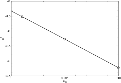
Figure 15: Results for the square of the mass of the fourth radial excitation of the pseudoscalar meson in units of $\sigma$ for three values $0.01\sqrt{\sigma}$, $0.005\sqrt{\sigma}$ and $0.001\sqrt{\sigma}$ of the IR regulator $\mu_{\rm IR}$ and extrapolation to the IR limit $\mu_{\rm IR}=0$.

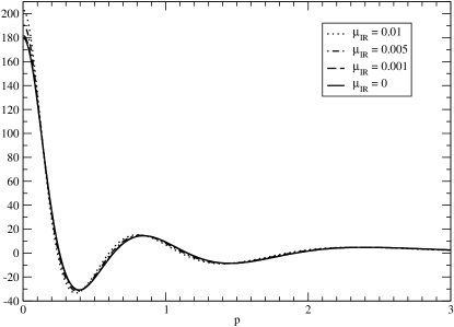
Figure 16: Component $\psi_{+}(p)$ of the wave function of the fourth radial excitation of the pseudoscalar meson for three small values of $\mu_{\rm IR}$ and its extrapolation to $\mu_{\rm IR}=0$. All quantities are given in appropriate units of $\sqrt{\sigma}$.

In a similar manner the IR limit of the wave functions can be obtained. In Figs. 15 we show as example the determination of the IR limit for the mass of the fourth radial excitation of the pseudoscalar meson. The forward-propagating component of the wave function of the same state is shown in Fig. 16 together with the extrapolated IR limit, which in this plot is hardly distinguishable from the result with $\mu_{\rm IR}=0.001\sqrt{\sigma}$.

The systems of integral equations (89), (93) and (99) are numerically solved by expanding the functions $h,g$ (respectively $h_{1},g_{1},h_{1},g_{2}$) in a finite set $(\varphi_{i},i=1,\ldots,N)$ of basis functions. In the following we show details for mesons of category 1: With

$$h(p) = \sum\limits_{i=1}^{N}c^{h}_{i}\varphi_{i}(p),$$ (114a)

$$\frac{\mu}{2}g(p) = \sum\limits_{i=1}^{N}c^{g}_{i}\varphi_{i}(p),$$ (114b)

one ends up with

$$A(\mu)\left(\begin{array}[]{c}\displaystyle\vec{c}^{h}\\ \displaystyle\vec{c}^{g}\end{array}\right)=B(\mu)\left(\begin{array}[]{c}\displaystyle\vec{c}^{h}\\ \displaystyle\vec{c}^{g}\end{array}\right),$$ (115)

where the real symmetric $2N\times 2N$ matrices $A(\mu)$ and $B(\mu)$ have the block structure

$$A(\mu) = \left(\begin{array}[]{cc}\displaystyle A^{hh}&\displaystyle 0\\ \displaystyle 0&\displaystyle A^{gg}(\mu)\end{array}\right)$$ (118)

$$B(\mu) = \left(\begin{array}[]{cc}\displaystyle B^{hh}&\displaystyle B^{hg}(\mu)\\ \displaystyle B^{gh}(\mu)&\displaystyle B^{gg}(\mu)\end{array}\right)$$ (121)

with symmetric real $N\times N$ matrices $A^{hh}$, $A^{gg}(\mu)$, $B^{hh}$ and $B^{gg}(\mu)$ and real $N\times N$ matrices $B^{hg}(\mu)$ and $B^{gh}(\mu)$ with $B^{hg}(\mu)^{T}=B^{gh}(\mu)$. The matrix elements are given by

$$A^{hh}_{ij}=\int\frac{d^{3}p}{(2\pi)^{3}}\varphi_{i}(p)\omega(p)\varphi_{j}(p),$$ (122)

$$A^{gg}_{ij}(\mu)=\int\frac{d^{3}p}{(2\pi)^{3}}\varphi_{i}(p)\left[\omega(p)-\frac{\mu^{2}}{4\omega(p)}\right]\varphi_{j}(p),$$ (123)

$$B^{hh}_{ij}=\frac{1}{2}\int\frac{d^{3}pd^{3}q}{(2\pi)^{6}}\varphi_{i}(p)V(k)P_{J}(\hat{p}\cdot\hat{q})\varphi_{j}(q),$$ (124)

$$B^{hg}_{ij}(\mu)=B^{gh}_{ji}(\mu)=\frac{\mu}{4}\int\frac{d^{3}pd^{3}q}{(2\pi)^{6}}\varphi_{i}(p)\frac{V(k)}{\omega(q)}P_{J}(\hat{p}\cdot\hat{q})\varphi_{j}(q),$$ (125)

$$B^{gg}_{ij}(\mu) = \frac{1}{2}\int\frac{d^{3}pd^{3}q}{(2\pi)^{6}}\varphi_{i}(p)V(k)$$ (126)

$$\times \left[\frac{M(p)M(q)P_{J}(\hat{p}\cdot\hat{q})+pq\left(\frac{J+1}{2J+1}P_{J+1}(\hat{p}\cdot\hat{q})+\frac{J}{2J+1}P_{J-1}(\hat{p}\cdot\hat{q})\right)}{\bar{\omega}(p)\bar{\omega}(q)}+\frac{\mu^{2}}{4\omega(p)\omega(q)}P_{J}(\hat{p}\cdot\hat{q})\right]\varphi_{j}(q).$$

One can drop or add terms of order ${\cal O}(\mu_{\rm IR})$ which leads to different results at finite $\mu_{\rm IR}$ but leaves the IR limit invariant (see the discussion on the IR limit of the BSE above). For instance one can drop the $\mu$-dependent terms in $A^{gg}(\mu)$ and $B^{gg}(\mu)$ or replace (125) by

$$B^{hg}_{ij}(\mu)=B^{gh}_{ji}(\mu)=\frac{\mu}{2}\int\frac{d^{3}p}{(2\pi)^{3}}\varphi_{i}(p)\varphi_{j}(p).$$ (127)

We have checked that these modifications indeed give — up to insignificant numerical errors — the same extrapolated IR limits. All results presented in this paper have been calculated with the exact expressions (122)–(126) for finite $\mu_{\rm IR}$. By introducing a multiplicative parameter $\lambda(\mu)$ on its right hand side, Eq. (115) becomes a generalized eigenvalue problem which can be solved with standard linear algebra methods yielding $2N$ eigenvalues $\lambda_{i}(\mu)$. The masses $\mu_{i}$ ($i=1,\ldots,K$) of the $K$ lowest lying mesons with given spin are then found by solving $\lambda_{i}(\mu_{i})=1$ for the lowest $K$ eigenvalues. The corresponding eigenvectors give the coefficients in the expansion (114) in each case. Finally the functions $h$ and $g$ have to be normalized according to (42). The spectra and wave functions of mesons of categories 2 and 3 are found in an analogous manner. As basis functions we take

$$\varphi_{i}(p)=p^{L}\exp(-\alpha_{i}p^{2}),$$ (128)

where $L=J$ for mesons of category 1 and 3 and $L=|J-1|$ for mesons of category 2. With properly chosen parametrs $\alpha_{i}$ a number of $N=20$ basis functions is sufficient for a satisfactory numerical accuracy of masses and wave functions of all states considered in this work.

References

- (1) M. Gell-Mann and M. Levy. Nuovo Cimento, 16, 705 (1960); B. W. Lee, Chiral dynamics, Gordon and Breach, NY 1972.
- (2) Y. Nambu and G. Jona-Lasinio, Phys. Rev. 122, 345 (1961); Phys. Rev. 124, 246 (1961).
- (3) B. L. Ioffe, Nucl. Phys. B 188, 317 (1981); E: B 191, 591 (1981).
- (4) L. Ya. Glozman, Phys. Lett. B 475, 329 (2000).
- (5) T. D. Cohen and L. Ya. Glozman, Phys. Rev. D 65, 016006 (2002); Int. J. Mod. Phys. A 17, 1327 (2002).
- (6) L. Ya. Glozman, Phys. Lett. B 541 (2002) 115.
- (7) L. Ya. Glozman, Phys. Lett. B 539 (2002) 257; Phys. Lett. B 587 (2004) 69.
- (8) L. Ya. Glozman, Int. J. Mod. Phys. A. 21 (2006) 475.
- (9) L. Ya. Glozman, A. V. Nefediev, J.E.F.T. Ribeiro, Phys. Rev. D 72 (2005) 094002.
- (10) A. Le Yaouanc, L. Oliver, O. Pene, and J. C.Raynal, Phys. Rev. D 29 (1984) 1233; 31 (1985) 137.
- (11) G. ’t Hooft, Nucl. Phys. B 75 (1974) 461; I. Baars, M. B. Green, Phys. Rev. D 17 (1978) 537.
- (12) Yu. S. Kalashnikova, A. V. Nefediev, J.E.F.T. Ribeiro, Phys. Rev. D 72 (2005) 034020.
- (13) R. F. Wagenbrunn, L. Ya. Glozman, Phys. Lett. B 643, 98 (2006).
- (14) T. D. Cohen and L. Ya. Glozman, Mod. Phys. Lett. A21 (2006) 1939.
- (15) R. L. Jaffe, D. Pirjol, A. Scardicchio, hep-ph/0602010; Phys. Rev. D 74 (2006) 057901.
- (16) L. Ya. Glozman, A. V. Nefediev, Phys. Rev. D 73 (2006) 074018.
- (17) M. Shifman, A. Vainstein, to be published
- (18) A. V. Nefediev, J. E. F. T. Ribeiro, A. P. Szczepaniak, hep-ph/0610430.
- (19) S.S. Afonin, Eur. Phys. J. A 29, 327 (2006).
- (20) M. Shifman, in: ”Quark-Hadron Duality and the Transition to pQCD”, Eds. A. Fantoni, S. Liuti, and O. Rondon (World Scientific, Singapore, 2006), pp. 171-192 (hep-ph/0507246).
- (21) O. Cata, M. Golterman, and S. Peris, Phys. Rev. D 74 (2006) 016001.
- (22) E. Swanson, Phys. Lett. B 582 (2004) 167; N. Ligterink and E. S. Swanson, Phys. Rev. C 69 (2004 ) 025204.
- (23) T. DeGrand, Phys. Rev. D 64 (2004) 074024.
- (24) T. D. Cohen, Nucl. Phys. A775 (2006) 89.
- (25) S. L. Adler and A. C. Davis, Nucl. Phys. B 244 (1984) 469.
- (26) R. Alkofer and P. A. Amundsen, Nucl. Phys. B 306 (1988) 305.
- (27) P. Bicudo and J. E. Ribeiro, Phys. Rev. D 42 (1990) 1611; 42 (1990) 1625.
- (28) P. J. A. Bicudo and A. V. Nefediev, Phys. Rev. D 68 (2003) 065021.
- (29) F. J. Llanes-Estrada and S. R. Cotanch, Phys. Rev. Lett., 84 (2000) 1102.
- (30) R. Alkofer, M. Kloker, A. Krassnigg, and R. F. Wagenbrunn, Phys. Rev. Lett. 96 (2006) 022001.
- (31) V. N. Gribov, Nucl. Phys. B 139, 1 (1978).
- (32) N. H. Christ and T. D. Lee, Phys. Rev. D 22 (1980) 939.
- (33) J. R. Finger and J. E. Mandula, Nucl. Phys. B 199 (1982) 168; J. Govaerts, J. E. Mandula, J. Weyers, Nucl. Phys. B 237 (1984) 59.
- (34) D. Zwanziger, Phys. Rev. D 70 (2004) 094034.
- (35) A. P. Szczepaniak and E. Swanson, Phys. Rev. D 65 (2002) 025012.
- (36) C. Feuchter and H. Reinhardt, Phys. Rev. D 70 (2004) 105021; H. Reinhardt and C. Feuchter, Phys. Rev. D 71 (2005) 105002; D. Epple, H. Reinhardt, W. Schleinfenbaum, hep-th/0612241.
- (37) J. Greensite, Š. Olejník, and D. Zwanziger, Phys. Rev. D 69 (2004) 074506.
- (38) A. Nakamura and T. Saito, Prog. Theor. Phys. 115 (2006) 189.
- (39) V. L. Morgunov, A. V. Nefediev, Yu. A. Simonov, Phys. Lett. B 459 (1999) 653.