Pion condensation in a two-flavour NJL model:
the role of charge neutrality

Abstract

We study pion condensation and the phase structure in a two-flavour Nambu–Jona-Lasinio model in the presence of baryon chemical potential $\mu$ and isospin chemical potential $\mu_{I}$ at zero and finite temperature. There is a competition between the chiral condensate and a Bose-Einstein condensate of charged pions. In the chiral limit, the chiral condensate vanishes for any finite value of the isospin chemical potential, while there is a charged pion condensate that depends on the chemical potentials and the temperature. At the physical point, the chiral condensate is always nonzero, while the charged pion condensate depends on $\mu_{I}$ and $T$. For $T=\mu=0$, the critical isospin chemical potential $\mu_{I}^{c}$ for the onset of Bose-Einstein condensation is always equal to the pion mass. For $\mu=0$, we compare our results with chiral perturbation theory, sigma-model calculations, and lattice simulations.

Finally, we examine the effects of imposing electric charge neutrality and weak equilibrium on the phase structure of the model. In the chiral limit, there is a window of baryon chemical potential and temperature where the charged pions condense. At the physical point, the charged pions do not condense.

1 Introduction

There has been a tremendous effort in recent years to map out the phase diagram of QCD as a function of temperature and baryon chemical potential [1, 2, 3, 4, 5, 6, 7]. It is generally accepted that one can calculate the properties of strongly interacting matter at asymptotically high temperature or at asymptotically high densities using perturbative QCD.

At sufficiently high density and low temperature, we know that QCD is in the colour-flavour locked (CFL) phase. This state is a colour superconducting state because the quarks form Cooper pairs in analogy to electrons in an ordinary superconductor. In this case, the original symmetry group of QCD, $SU(3)_{\rm c}\times SU(3)_{L}\times SU(3)_{R}\times U(1)_{B}$, is broken down to $SU(3)_{c+L+R}$ which is a linear combination of the generators of the original group. This linear combination locks rotation in colour space to rotations in flavour space and this has given the name to the phase. In the CFL phase there is an octet of Goldstone modes which arises from the breaking of chiral symmetry and a singlet arising from the breaking of the baryon-number conserving group $U(1)_{B}$. The CFL phase is a superfluid due to the breaking of the global $U(1)_{B}$ symmetry. This is analogous to the superfluidity encountered in in condensed-matter systems such as ⁴He. At very high densities, all nine modes are effectively massless since one can ignore the quark masses. This implies that the low-energy properties of the CFL phase can be described in terms of an effective field theory for the massless mesons [8, 9, 10, 11]. At moderate densities, one cannot neglect the quark masses and chiral symmetry is broken explicitly. Thus only the superfluid mode is exactly massless, while the the other mesons acquire masses. The lightest massive modes are expected to be the charged and neutral kaons and if the chemical potentials are large enough, there is a transition to a Bose condensed phase. Bose condensation of kaons in the CFL phase has been studied in detail in Refs. [12, 13, 14, 15, 16, 17, 18, 19, 20, 21, 22].

QCD at finite baryon chemical potential $\mu_{B}$ is not accessible by Monte Carlo simulations due to the complex fermion determinant. This is in contrast to QCD at finite isospin chemical potential $\mu_{I}$ (still at zero $\mu_{B}$) where lattice simulations are possible since the functional determinant is real. Thus this is a system whose phase diagram one can study on the lattice as a function of a conserved charge.

Lattice simulations [23, 24, 25] suggest that there is a deconfinement transition of pions at high temperature and low density, and Bose-Einstein condensation of charged pions at high isospin density and low temperature. In fact, the deconfinement transition and the transition to a charged pion condensate seem to coincide. The deconfinement transition is found by measuring the Polyakov loop and the measurements show a sharp increase (indicating deconfinement) at approximately the same temperature as the onset of pion condensation.

Pion condensation and the phase diagram of two-flavour QCD have been investigated using chiral perturbation theory [26, 27, 28], ladder QCD [29], the chiral quark model [30], the linear sigma models [31, 32, 33, 34, 35, 36], NJL models [33, 37, 38, 39, 40, 41, 42, 43], and Polyakov-loop NJL models [44, 45]. The PNJL models suggest that deconfinement and the onset of Bose-Einstein condensation are two different transitions. Very recently, Abuki et al [46] have considered the possibility of probing the phase diagram of electrically neutral QCD at finite isospin chemical potential using an equilibrated gas of neutrinos. They found that a condensate of charged pions arises at large enough neutrino densities and small baryon densities, and that at even larger neutrino densities there is condensation of charged kaons as well.

We note in passing the similarity between three-colour QCD at finite $\mu_{I}$ and two-colour QCD at finite $\mu_{B}$ [23]. The correspondence is given by identifying $\mu_{I}/2$ with $\mu_{B}$, the charged pion condensate with the diquark condensate, and the isospin density with the quark density.

Bose-condensed states or colour-superconducting states may be found in the interior of compact stars if the density is high enough. In contrast to hadronic matter in heavy-ion collisions, bulk matter in compact stars must (on average) be electrically neutral and so a neutrality constraint must be imposed [47, 48]. Similarly, bulk matter must be colour neutral and if the system is in a colour superconducting phase, one sometimes has to impose this constraint explicitly. It is automatically satisfied if one uses the QCD Lagrangian, but this is not so if one describes the system using NJL-type models. This is due to the fact that there are no gauge fields in this model and the $SU(N_{c})$ colour symmetry is global [18, 49, 50, 51].

The advantage of models with quarks as microscopic degrees of freedom, such as the NJL model, is that one can investigate simultaneously the effects of finite baryon chemical potential and isospin chemical potential. In the present paper, we consider the two-flavour NJL model at finite baryon chemical potential and isospin chemical potential. We compute the phase diagram at zero and finite temperature as a function of these variables. We restrict ourselves to sufficiently low values of the baryon chemical potential such that there are no superconducting phases [48, 52]. We also investigate the effects on the phase diagram by imposing electric charge neutrality and $\beta$-equilibrium. Our work is a generalization of the papers by Ebert and Klimenko [38, 39] to finite temperature and finite pion mass.

The article is organized as follows. In Sec. 2, we discuss the Lagrangian and the gap equations of NJL model. In Sec. 3, we discuss the phase diagram at zero as well as finite temperature. In Sec. 4, we discuss the issues of charge neutrality and $\beta$-equlibrium. In Sec. 5, we investigate the phase diagram at zero and finite temperature imposing charge neutrality and $\beta$-equlibrium. In Sec. 6, we summarize and conclude.

2 Lagrangian and Gap equations

In this section, we discuss the properties of the Lagrangian of the two-flavour NJL model. The Lagrangian can be written as [53]

$${\cal L} = {\cal L}_{0}+{\cal L}_{1}+{\cal L}_{2}\;,$$ (1)

where the various terms are

$${\cal L}_{0} = \bar{\psi}(i\gamma^{\mu}\partial_{\mu}-m_{0})\psi\;,$$ (2)

$${\cal L}_{1} = G_{1}\left[(\bar{\psi}\psi)^{2}+(\bar{\psi}\boldsymbol{\tau}\psi)^{2}+(\bar{\psi}i\gamma_{5}\psi)^{2}+(\bar{\psi}i\gamma_{5}\boldsymbol{\tau}\psi)^{2}\right]\;,$$ (3)

$${\cal L}_{2} = G_{2}\left[(\bar{\psi}\psi)^{2}-(\bar{\psi}\boldsymbol{\tau}\psi)^{2}-(\bar{\psi}i\gamma_{5}\psi)^{2}+(\bar{\psi}i\gamma_{5}\boldsymbol{\tau}\psi)^{2}\right]\;.$$ (4)

Here, $m_{0}$ is the quark-mass matrix, which is diagonal in flavour space and contains the bare quark masses $m_{u}$ and $m_{d}$. Moreover, ${\boldsymbol{\tau}}=(\tau_{1},\tau_{2},\tau_{3})$ where $\tau_{i}$ ($i=1,2,3$) are the Pauli matrices. $G_{1}$ and $G_{2}$ are coupling constants. The quark field $\psi$ is an isospin doublet

$$\psi=\left(\begin{array}[]{c}u\\ d\\ \end{array}\right)\;.$$ (7)

In the following, we take $m_{u}=m_{d}$. The Lagrangian (1) has a global $SU(N_{c})$ symmetry as well as a $U(1)_{B}$ baryon symmetry. The latter reflects baryon number conservation. In the chiral limit, the Lagrangian (1) has an $SU(2)_{L}\times SU(2)_{R}$ symmetry. Away from the chiral limit, this symmetry is reduced to $SU(2)_{L+R}$ isospin symmetry. ${\cal L}_{1}$ has an additional $U(1)_{A}$ axial symmetry. ${\cal L}_{2}$ is ’t Hooft’s instanton-induced interaction term and breaks explicitly the $U(1)_{A}$ axial symmetry of ${\cal L}_{1}$ [54, 55]. In the following, we shall limit ourselves to study the standard NJL Lagrangian by choosing $G_{1}=G_{2}\equiv G/2$ [53] and so Eq. (1) reduces to

$${\cal L} = \bar{\psi}(i\gamma^{\mu}\partial_{\mu}-m_{0})\psi+G\left[(\bar{\psi}\psi)^{2}+(\bar{\psi}i\gamma_{5}\boldsymbol{\tau}\psi)^{2}\right]\;.$$ (8)

We can characterize the system described by the Lagrangian (8) by the expectation values of the different conserved charges associated with the continuous symmetries. For each conserved charge $Q_{i}$, we introduce a chemical potential $\mu_{i}$. Note, however, that it is possible to specify the expectation values of different charges simultaneously only if they commute. In the present case, we introduce a chemical potential $\mu_{B}$ associated with the $U(1)_{B}$ baryon symmetry, as well as a chemical potential $\mu_{I}$ associated with the third component of the $SU(2)_{L+R}$ isospin group. This is done by adding to the Lagrangian (8), the terms

$${\cal L}_{B} = \mu_{B}\bar{\psi}\gamma^{0}B\psi\;,$$ (9)

$${\cal L}_{I} = \mu_{I}\bar{\psi}\gamma^{0}I_{3}\psi\;,$$ (10)

where $B={\rm diag}(1/3,1/3)$ and $I_{3}=\tau_{3}/2$. We can then write the Lagrangian as

$$\mathcal{L}=\bar{\psi}\left[i\gamma^{\mu}\partial_{\mu}-m_{0}+\mu\gamma^{0}+\delta\mu\gamma^{0}\tau_{3}\right]\psi+G\left[(\bar{\psi}\psi)^{2}+(\bar{\psi}i\gamma^{5}\tau_{i}\psi)^{2}\right]\;,$$ (11)

where we have defined the quark chemical potential $\mu$ as well as $\delta\mu$ by

$$\mu \equiv \frac{\mu_{B}}{3}\;,$$ (12)

$$\delta\mu \equiv {\mu_{I}\over 2}\;.$$ (13)

In the remainder of the paper we assume $\mu\geq 0$ and $\delta\mu\geq 0$ for simplicity. In terms of the chemical potentials for the $u$ and the $d$-quarks, $\mu_{u}$ and $\mu_{d}$, the chemical potentials $\mu$ and $\delta\mu$ can be written as

$$\mu = {1\over 2}(\mu_{u}+\mu_{d})\;,$$ (14)

$$\delta\mu = {1\over 2}(\mu_{u}-\mu_{d})\;.$$ (15)

In the chiral limit, the inclusion of the isospin chemical potential breaks the $SU(2)_{L}\times SU(2)_{R}$-symmetry of the Lagrangian to $U(1)_{L}\times U(1)_{R}$. At the physical point, it breaks the $SU(2)_{L+R}$-symmetry down to $U(1)_{L+R}$.

From the path-integral representation of the free energy density $\Omega$

$$e^{-\beta V\Omega} = \int{\cal D}\psi^{*}{\cal D}\psi e^{-\int_{0}^{\beta}d\tau\int d^{3}x\cal L}\;,$$ (16)

the expression for the charge density $Q_{i}$ associated with the chemical potential $\mu_{i}$ can be written as

$$Q_{i} = -{\partial{\Omega}\over\partial\mu_{i}}\,.$$ (17)

We next introduce the auxiliary fields $\sigma$ and $\pi_{i}$ by

$$\sigma = -2G\bar{\psi}\psi\;,$$ (18)

$$\pi_{i} = -2G\bar{\psi}i\gamma_{5}\tau_{i}\psi\;.$$ (19)

The Lagrangian (11) can now compactly be written as

$${\cal L} = \bar{\psi}\left[i\gamma^{\mu}\partial_{\mu}-m_{0}+\mu\gamma^{0}+\delta\mu\gamma^{0}\tau_{3}-\sigma-i\gamma^{5}\pi_{a}\tau_{a}\right]\psi$$ (20)

$$-{1\over 4G}\left(\sigma^{2}+\pi_{a}\pi_{a}\right)\;.$$

The original Lagrangian (11) can be recovered by using the equations of motion for the auxiliary fields $\sigma$ and $\pi_{i}$ to eliminate them from Eq. (20). The Lagrangian is now bilinear in the quark fields and so we can integrate them out exactly. We then obtain the following effective action for the composite fields $\sigma$ and $\pi_{i}$

$$S_{\rm eff} = -{1\over 2}N_{c}{\rm Tr\log}\left[i\gamma^{\mu}\partial_{\mu}-m_{0}+\mu\gamma^{0}+\delta\mu\gamma^{0}\tau_{3}-\sigma-i\gamma^{5}\pi_{a}\tau_{a}\right]$$ (21)

$$-\int d^{3}x\int_{0}^{\beta}d\tau{1\over 4G}\left(\sigma^{2}+\pi_{a}\pi_{a}\right),$$

where ${\rm Tr}$ denotes the trace and is over Dirac indices as well as space-time.

We next introduce a nonzero expectation value for the fields $\sigma$ and $\pi_{1}$ to allow for a chiral condensate and a charged pion condensate. The fields are then written as

$$\sigma = -2G\langle\bar{\psi}\psi\rangle+\tilde{\sigma}\;,$$ (22)

$$\pi_{1} = -2G\langle\bar{\psi}i\gamma^{5}\tau_{1}\psi\rangle+\tilde{\pi}_{1}\;,$$ (23)

where $\tilde{\sigma}$ and $\tilde{\pi}_{1}$ are quantum fluctuating fields. In the mean-field approximation, we neglect the fluctuations of the quantum fields $\tilde{\sigma}$ and $\tilde{\pi}_{1}$ in the functional determinant. This approximation coincides with the leading order of the $1/N_{c}$-expansion, where $N_{c}$ is the number of colours .

For notational simplicity, we introduce the quantities $M$ and $\rho$ given by

$$M \equiv m_{0}-2G\langle\bar{\psi}\psi\rangle\;,$$ (24)

$$\rho \equiv -2G\langle\bar{\psi}i\gamma^{5}\tau_{1}\psi\rangle\;,$$ (25)

where $M$ is the constituent quark mass. Note that in the chiral limit, the chiral condensate breaks the $SU(2)_{L}\times SU(2)_{R}$ symmetry spontaneously down to $SU(2)_{L+R}$ in the usual manner. Moreover, we can always use the remaining $U(1)$-symmetry to rotate away any nonzero value of $\langle\bar{\psi}\gamma^{5}\tau_{2}\psi\rangle$.

Note that we have introduced a single chiral condensate and not separate chiral condensates $\langle\bar{u}u\rangle$ and $\langle\bar{d}d\rangle$ for the $u$ and the $d$ quarks. We have chosen $G_{1}=G_{2}$ and in this case the effective action (21) only depends on the sum of these condensates. In fact, it is easy to show that the two chiral condensates must be equal. This is in contrast to the calculations of Barducci et al [37], where the authors choose $G_{1}=G/2$ and $G_{2}=0$. In that case the effective action is not symmetric under permutation of the two chiral condensates and they are different. Our choice is motivated by the fact that $U(1)_{A}$ symmetry is broken in QCD due to instanton effects [56]. In fact, setting $G_{1}=G_{2}\neq 0$ in the present model means that axial symmetry is maximally violated. When $G_{2}=0$, on the other hand, the Lagrangian (1) is $U(1)_{A}$-symmetric.

Also note that we take the condensates $M$ and $\rho$ to be spacetime independent. Though it has been demonstrated that the phase diagram may contain phases where the condensates are non-uniform [57], also within the framework of the two-flavour NJL model [58, 59, 60, 61, 62], taking this possibility into account is beyond the scope of this study. Still, it would be interesting to see how these non-uniform phases are affected by imposing neutrality constraints.

Using standard techniques to evaluate the trace and using $\Omega=-S_{\rm eff}/\beta V$, where $\Omega$ is the thermodynamic potential and $V$ is the volume of the system, we obtain

$$\Omega = {(M-m_{0})^{2}+\rho^{2}\over 4G}-2N_{c}\int{d^{3}p\over(2\pi)^{3}}\bigg{\{}E_{\rho}^{-}+T\ln\left[1+e^{-\beta(E_{\rho}^{-}-\mu)}\right]$$ (26)

$$+T\ln\left[1+e^{-\beta(E_{\rho}^{-}+\mu)}\right]+E_{\rho}^{+}+T\ln\left[1+e^{-\beta(E_{\rho}^{+}-\mu)}\right]$$

$$+T\ln\left[1+e^{-\beta(E_{\rho}^{+}+\mu)}\right]\bigg{\}}\;,$$

where the energy $E^{\pm}_{\rho}$ is defined by

$$E^{\pm}_{\rho} = \sqrt{(E^{\pm})^{2}+\rho^{2}}$$ (27)

where

$$E^{\pm} = E\pm\delta\mu\;,$$ (28)

$$E = \sqrt{p^{2}+M^{2}}\;.$$ (29)

In the limit $T\rightarrow 0$, the thermodynamic potential (26) reduces to

$$\Omega = {(M-m_{0})^{2}+\rho^{2}\over 4G}-2N_{c}\int{d^{3}p\over(2\pi)^{3}}\bigg{\{}E_{\rho}^{-}+(\mu-E_{\rho}^{-})\theta(\mu-E_{\rho}^{-})$$ (30)

$$+E_{\rho}^{+}+(\mu-E_{\rho}^{+})\theta(\mu-E_{\rho}^{+})\bigg{\}}\;,$$

which is in agreement with the result of Ref. [38]. The values of $M$ and $\rho$ are found by minimizing the thermodynamic potential $\Omega$, that is by solving the following gap equations

$${\partial\Omega\over\partial M} = 0\;,$$ (31)

$${\partial\Omega\over\partial\rho} = 0\;.$$ (32)

Differentiating the effective potential (26) with respect to $M$ and $\rho$, we obtain the gap equations

$$0 = {M-m_{0}\over 2G}-2N_{c}M\int{d^{3}p\over(2\pi)^{3}}\bigg{\{}{E^{+}\over EE^{+}_{\rho}}[1-n(E^{+}_{\rho}-\mu)-n(E^{+}_{\rho}+\mu)]$$ (33)

$$+{E^{-}\over EE^{-}_{\rho}}[1-n(E^{-}_{\rho}-\mu)-n(E^{-}_{\rho}+\mu)]\bigg{\}}\;,$$

$$0 = {\rho\over 2G}-2N_{c}\rho\int{d^{3}p\over(2\pi)^{3}}\bigg{\{}{1\over E^{+}_{\rho}}[1-n(E^{+}_{\rho}-\mu)-n(E^{+}_{\rho}+\mu)]$$ (34)

$$+{1\over E^{-}_{\rho}}[1-n(E^{-}_{\rho}-\mu)-n(E^{-}_{\rho}+\mu)]\bigg{\}},$$

where $n$ is the Fermi-Dirac distribution,

$$n(E)=\frac{1}{e^{\beta E}+1}.$$ (35)

Taking the limit $T\rightarrow 0$, these equations reduce to those obtained by Ebert and Klimenko [38]:

$$0 = {M-m_{0}\over 2G}-2N_{c}M\int{d^{3}p\over(2\pi)^{3}}\left\{{\theta(E_{\rho}^{+}-\mu)E^{+}\over EE_{\rho}^{+}}+{\theta(E_{\rho}^{-}-\mu)E^{-}\over EE_{\rho}^{-}}\right\}\;,$$ (36)

$$0 = {\rho\over 2G}-2N_{c}\rho\int{d^{3}p\over(2\pi)^{3}}\left\{{\theta(E_{\rho}^{+}-\mu)\over E_{\rho}^{+}}+{\theta(E_{\rho}^{-}-\mu)\over E_{\rho}^{-}}\right\}\;.$$ (37)

The dispersion relations for the quasiparticles are determined by the zeros of the functional determinant in Eq. (21). One finds [38]

$$E_{u}=E_{\rho}^{-}-\mu\;,\hskip 28.45274ptE_{d}=E_{\rho}^{+}-\mu$$ (38)

$$E_{\bar{u}}=E_{\rho}^{-}+\mu\;,\hskip 28.45274ptE_{\bar{d}}=E_{\rho}^{+}+\mu\;.$$ (39)

It is easy to show that the dispersion relations for the $\bar{u}$ and $\bar{d}$-quarks are always gapped, while the dispersion relations for the $u$ and $d$-quarks can be gapped or ungapped depending on the values of $\mu$. In the chiral limit, it follows directly from the gap equations (33) and (34) that there are no nonzero values for $\mu$, $\delta\mu$, and $T$ for which $M$ and $\rho$ are nonzero simultaneously. In the pion-condensed phase the dispersion relations for $u$ and $d$-quarks then reduce to

$$E_{u} = \sqrt{(p-\delta\mu)^{2}+\rho^{2}}-\mu\;$$ (40)

$$E_{d} = \sqrt{(p+\delta\mu)^{2}+\rho^{2}}-\mu\;.$$ (41)

For the $u$-quark, the dispersion relation is gapped or ungapped according to

$$\rho > \mu\;,\hskip 28.45274pt{\rm gapped\,\,\,spectrum}\;,$$ (42)

$$\rho = \mu\;,\hskip 28.45274pt{\rm ungapped\,\,\,quadratic\,\,\,spectrum}\;,$$ (43)

$$\rho < \mu\;,\hskip 28.45274pt{\rm ungapped\,\,\,linear\,\,\,spectrum}\;.$$ (44)

The possibility of an ungapped quadratic quark spectrum in the context of dense baryonic matter was first discussed in Ref. [63]. The gaplessness of the $d$-quark is determined by the line that is defined implicitly by the equation $\mu=\sqrt{(\delta\mu)^{2}+\rho^{2}}$, which follows from Eq. (41). The window in the pion-condensed phase where the fermionic excitations are gapless is coined gapless pion condensation [38]. The situation here is analogous to what happens in colour superconductivity, except that in this case it is $\delta\mu$ that dictates the onset of gaplessness: $\delta\mu=\Delta$, where $\Delta$ is the superconducting gap [6, 64]. Moreover, in colour superconductivity $\delta\mu$ is called a stress parameter because it gives rise to a mismatch between the Fermi surfaces of the $u$ and the $d$-quarks, which imposes an extra energy cost (stress) on the formation of Cooper pairs. As long as the stress parameter is small enough compared to $\Delta$, BCS pairing can occur [64]. In the context of pion condensation, $\mu$ plays the role as a stress parameter since the mismatch is between the Fermi surfaces of the $u$ and $\bar{d}$-quarks. Similarly, if the stress parameter $\mu$ is small enough relative to $\rho$, pion condensation can occur. We will return to this point below.

The integrals appearing in Eqs. (26), (33), and (34) are ultraviolet divergent and one may impose a three-dimensional UV cutoff $\Lambda$ to regulate them. Alternatively, one can introduce a form factor [65], which falls off for large momenta. This ensures that the integrals converge in the ultraviolet. Given an ultraviolet cutoff $\Lambda$, the coupling constant $G$ and the quark mass $m_{0}$, we can use the Dyson equation for the quark propagator to determine the value for the chiral condensate in the vacuum. The Dyson equation reads [53]:

$$M=m_{0}+4N_{f}N_{c}G\int{d^{3}p\over(2\pi)^{3}}{M\over\sqrt{p^{2}+M^{2}}}\;,$$ (45)

where $N_{f}$ is the number of flavours and $N_{c}$ is the number of colours. In the remainder of the paper, we also set $N_{f}=2$,and $N_{c}=3$. This is simply the gap equation (33) in the vacuum, i.e. for $\mu=\delta\mu=0$.

3 Phase diagram

In this section, we study the phase diagram at zero and finite temperature without taking charge neutrality into account. Since we are not considering colour superconductivity, we restrict ourselves to quark chemical potentials $\mu<350$ MeV. Since we are using an ultraviolet cutoff of approximately $650$ MeV (see below), one should not trust results for the chemical potentials $\mu$ and $\delta\mu$ above approximately $400$ MeV. We therefore do not consider values above $\mu=350$ MeV and $\delta\mu=400$ MeV in the calculations. The equilibrium values of $M$ and $\rho$ are obtained by solving numerically the gap equations (33) and (34).

3.1 Chiral Limit

In the chiral limit, the current quark mass vanishes, $m_{0}=0$. For the numerical calculations, we choose an ultraviolet cutoff $\Lambda=650.9$ MeV and a coupling constant $G=5.04$ (GeV)^-2. Solving the Dyson equation (45), this gives a constituent quark mass in the vacuum of $M=309.9$ MeV.

We mentioned in the previous section that there are no values of $\mu$, $\delta\mu$, and $T$ such that $M$ and $\rho$ are simultaneously nonzero. In other words, the possible solutions to the gap equations are a) $M=\rho=0$, b) $M\neq 0,\;\rho=0$ and c) $\rho\neq 0,\;M=0$. In case a), the full symmetry of the Lagrangian is intact, while in case b) the $U(1)_{L}\times U(1)_{R}$ symmetry is broken spontaneously down to $U(1)_{L+R}$ by the chiral condensate. The breaking of the $U(1)$-symmetry gives rise to a conventional Goldstone mode In case c) the pion condensate breaks parity as well the $U(1)_{L}\times U(1)_{R}$ symmetry down to $U(1)_{AI_{3}}$. The latter transforms the left-handed and right-handed flavour doublet as $\psi_{L}\rightarrow e^{i\alpha\tau_{3}}\psi_{L}$, $\psi_{R}\rightarrow e^{-i\alpha\tau_{3}}\psi_{R}$. The breaking of the $U(1)$-symmetry gives rise to a conventional Goldstone boson with a linear dispersion relation for small values of the three-momentum. The ground state is therefore a pion superfluid . The dispersion relations for the composite fields $\sigma$ and $\pi$ in Eqs. (18)–(19) are found by first expanding the effective action (21) to second order in the quantum fluctuating field $\tilde{\sigma}$ and $\tilde{\pi}_{i}$. This gives rise to a $4\times 4$ fluctuation matrix $\Gamma(\omega,p)$, where the solutions to $\det\Gamma(\omega,p)=0$ determine the dispersion relations $\omega(p)$. Details can be found in Ref. [39]. At finite chemical potential there is a mixing between the fields $\tilde{\pi}_{1}$ and $\tilde{\pi}_{2}$ and one of the linear combinations is massless [38].

The pion condensate of the two-flavour NJL model at zero temperature is shown in Fig. 1. It is worth noting that along the $\mu$-axis, i.e for $\delta\mu=0$, the effective potential no longer depends on $M$ and $\rho$ separately, but rather on the combination $M^{2}+\rho^{2}$ [39]. The effective potential then has the usual mexican-hat shape with infinitely many equivalent vacua, where we can choose anyone we wish. The chiral condensate can be rotated into pseudoscalar condensates via the axial flavour transformations

$$\psi\rightarrow e^{i\theta_{a}\gamma_{5}\tau_{a}}\psi\;,\hskip 28.45274pta=1,2,3\;.$$ (46)

This is analogous to what happens in colour superconductivity, where diquark condensates are rotated into pseudoscalar diquark ones via rotations similar to those in Eq. (46) [12]. At finite quark mass or finite isospin chemical potential, the system becomes unstable against developing a nonzero pion condensate. At vanishing isospin chemical potential, parity is conserved in QCD and to enforce this we choose $\rho=0$ along the line $\delta\mu=0$. Consequently, the chiral condensate is nonvanishing and chiral symmetry is broken along the line $\delta\mu=0$. Fig. 1 shows that the charged pions condense for any nonzero value of the isospin chemical potential This result is in accordance with that of Ebert and Klimenko [38] and calculations in the linear sigma model at finite isospin chemical potential [33, 34]. Finally, we notice that the phase transition from the pion condensed phase to the chirally symmetric phase is first order. Notice that the critical isospin chemical potential $\delta\mu$ is decreasing as a function of $\mu$.

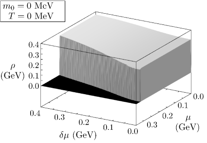
Figure 1: Pion condensate in the chiral limit as a function of quark chemical potential $\mu$ and $\delta\mu$ at zero temperature.

In Fig. 2, we show the pion condensate as a function of quark chemical potential and isospin chemical potential at $T=150$ MeV. The region of pion condensation is smaller than at $T=0$ and the transition to a chirally symmetric phase is now second order everywhere.

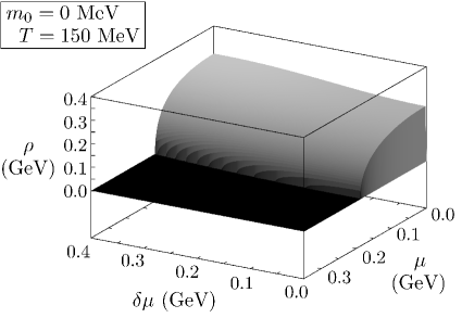
Figure 2: Pion condensate in the chiral limit as a function of $\mu$ and $\delta\mu$ for $T=150$ MeV.

In Fig. 3, we show the pion condensate in the chiral limit as a function of $\mu$ and $T$ for fixed value of isospin chemical potential, $\delta\mu=200$ MeV. As the temperature and the quark chemical potential increase, the region of pion condensation decreases. For $T=0$, the transition is first order. There is a line of first-order transitions starting at $T=0$ which ends at a critical point given by $T=0.11$ GeV and $\mu=0.22$ GeV. The transition is of second order for larger values of $T$ and smaller values of $\mu$.

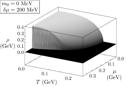
Figure 3: Pion condensate in the chiral limit as a function quark chemical $\mu$ potential and temperature $T$ for $\delta\mu=200$ MeV.

As mentioned above, the quark chemical potential induces a stress in the system and for sufficiently large values of $\mu$ it is no longer energetically favourable to form a Bose condensate of charged pions. This is clearly seen in Fig. 4, where we have plotted the thermodynamic potential $\Omega(\rho)$ minus $\Omega(\rho=0)$ for three different values of $\mu$ with $\delta\mu=200$ MeV and $T=0$. From this figure it is evident that the transition is first order.

Figure 4: $\Omega(\rho)-\Omega(\rho=0)$ in the chiral limit at $T=0$ as a function of $\rho$ for $\delta\mu=200$ MeV and three different values of $\mu$. Solid line: 100 MeV, dashed line: 275.87MeV, and dotted line: 350 MeV.

3.2 Physical point

At the physical point, we choose the parameters $m_{0}=5.5$ MeV, $\Lambda=650.9$ MeV, and $G=5.04\;({\rm GeV})^{-2}$. Solving the Dyson equation (45), this gives a constituent quark vacuum mass $M=325.2$ MeV, and the model reproduces the pion mass of $m_{\pi}=140$ MeV.

Due to the nonzero current quark mass, the chiral condensate $M$ will always be nonzero and so chiral symmetry is never restored. For sufficiently high temperature or chemical potentials, the chiral condensate goes towards zero since the temperature-independent value of $m_{0}$ becomes irrelevant.

The two possible solutions of the gap equations are therefore a) $\rho=0$ and b) $\rho\neq 0$. In the case a) the full symmetry of the Lagrangian is intact, while in case b) parity and the $U(1)_{L+R}$ symmetry are spontaneously broken. In the latter case, there is a conventional Goldstone mode and the ground state is a pion superfluid.

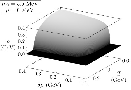
Figure 5: Pion condensate for $\mu=0$ as a function of $T$ and $\delta\mu$.

In Fig. 5, we show the pion condensate as a function of $T$ and $\delta\mu$ for $\mu=0$. The transition is second order everywhere with mean-field critical exponents, which is in agreement with the analysis using chiral perturbation theory [26, 27]. However, lattice calculations [23] suggest that the transition is first order for $\mu_{I}$ large enough. The line of first-order transitions ends at a tricritical point and the line of second-order transitions extends down to $T=0$. This discrepancy between mean-field calculations and lattice calculations is most likely due to shortcomings of mean-field theory itself. Lattice simulations also suggest that the transition to a Bose-Einstein condensed state coincides with the deconfinement phase transition to a quark-gluon plasma.

In Fig. 6, we show the pion condensate as a function of $\mu$ and $\delta\mu$ at the physical point for $T=0$. Along the axis $\mu=0$, the transition to the pion condensed phase occurs at $\delta\mu_{\rm c}=m_{\pi}/2=70$ MeV. The phase transition for $\mu=0$ is second order. The transition remains second order for $\delta\mu^{c}$ smaller than approximately $80$ MeV. For larger values of $\delta\mu$ it turns into a first-order transition. This is also shown in Fig. 7, where the solid curve shows a first-order transition ending at a critical point, while the dashed line indicates a second order transition. This figure is very similar to Fig. 3 of Ref. [43].

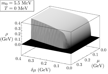
Figure 6: Pion condensate at the physical point as a function of quark chemical potential $\mu$ and $\delta\mu$ at zero temperature.

The results for the pion condensate are in qualitative agreement with that obtained by Barducci et al [37]. Quantitative difference are due to different quark-antiquark interaction terms in the Lagrangian as well as different ways of regulating the loop integrals.

Figure 7: Phase diagram at the physical point at $T=0$. The solid curve indicates a first-order transition which ends at a critical point. The dashed curve indicates a second-order transition.

In Fig. 8, we show the chiral and pion condensates as functions of the isospin chemical potential for $\mu=T=0$. The chiral condensate is constant from $\delta\mu=0$ to $\delta\mu\approx m_{\pi}/2$, after which it drops rapidly towards zero at large $\delta\mu$. This behaviour is in agreement with the lattice simulations of Kogut and Sinclair [23] and the sigma-model calculations of He et al [33]. We notice the onset of pion condensation at $\delta\mu\approx m_{\pi}/2$ and that the condensate increases rapidly thereafter. This illustrates the competition between the two condensates.

Figure 8: Pion condensate (dashed curve) and chiral condensate (solid curve) of the two-flavour NJL model at the physical point as a function of $\delta\mu$ at $\mu=T=0$.

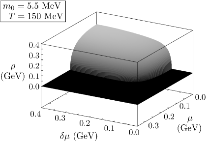
Figure 9: Pion condensate of the two-flavour NJL model at the physical point as a function of $\mu$ and $\delta\mu$ for $T=150$MeV.

In Fig. 9, we show the pion condensate as a function of $\mu$ and $\delta\mu$ at the physical point for $T=150$ MeV. The region of Bose condensation becomes smaller as the temperature increases, as expected. The phase transition is now second order everywhere.

In Fig. 10 we show the phase diagram of the two-flavour NJL model as a function of $T$ and $\delta\mu$ for $\mu=0$. The solid line is the chiral limit and the dashed line is the at the physical point. We note that the two curves are approaching each other for large values of $\delta\mu$, as expected.

Figure 10: Phase diagram as a function of $\delta\mu$ and $T$ for $\mu=0$. The solid line is the chiral limit and the dashed line is at the physical point.

In Fig. 11, we show the chiral condensate as a function of $\mu$ and $\delta\mu$ at the physical point and for $T=0$. The chiral condensate goes to zero as the chemical potentials become large.

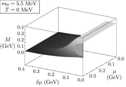
Figure 11: Chiral condensate as a function of quark chemical potential $\mu$ and $\delta\mu$ for zero temperature.

4 Electric Charge Neutrality and $\beta$-equilibrium

In the previous section, we have calculated the phase diagram by finding the solutions to the gap equations (31) and (32). Dense matter inside stars should be neutral with respect to electric as well as colour charge, otherwise one would pay an enormous energy price [47, 48]. Since we are not considering colour superconducting phases, colour neutrality is automatically satisfied, while we have to impose electric charge neutrality.

In addition to charge neutrality, matter should also be in $\beta$ equilibrium, that is, weak-interaction processes such as

$$u\leftrightarrow d+e^{+}+\nu\;,$$ (47)

should go with the same rate in both directions. If we assume that the neutrinos can leave the system, their chemical potential $\mu_{\nu}$ vanishes. In chemical equlibrium, Eq. (47) then implies

$$\mu_{u} = \mu_{d}-\mu_{e}\;.$$ (48)

The quark chemical potentials $\mu_{u}$ and $\mu_{d}$, and the electron chemical potential $\mu_{e}$ can be written in terms of the quark chemical potential $\mu$ and the electric chemical potential $\mu_{Q}$ as

$$\mu_{u} = \mu+{2\over 3}\mu_{Q}\;,$$ (49)

$$\mu_{d} = \mu-{1\over 3}\mu_{Q}\;,$$ (50)

$$\mu_{e} = -\mu_{Q}\;,$$ (51)

and so the system can be described in terms of the two independent chemical potentials $\mu$ and $\mu_{Q}$. In order to impose the constraint of charge neutrality, we additionally require that

$${\partial\Omega\over\partial\mu_{Q}} = 0\;.$$ (52)

The constraint (52) implies that there is only one independent chemical potential, for example $\mu$. Once we have picked a value for $\mu$, the solutions to the gap equations (31) and (32) and the neutrality constraint (52) determine the chiral condensate $M$, the charged pion condensate $\rho$, and the electric chemical potential $\mu_{Q}$.

Note that the chemical potential appearing in Eq. (26) is half the the sum of the quark chemical potentials $\mu_{u}$ and $\mu_{d}$, and so according to Eqs. (49) and (50), we need to make the substitution $\mu\rightarrow\tilde{\mu}=\mu+\mu_{Q}/6$. In the remainder, we also replace $\delta\mu$ by $\mu_{Q}/2$, which follows from Eqs. (15), (49), and (50).

In the following, we describe the electrons by a noninteracting Fermi gas. We then add to the Lagrangian (11), the term

$${\cal L}_{\rm electrons} = \bar{\psi}_{e}\left(\gamma^{\mu}\partial_{\mu}+\gamma^{0}\mu_{e}e-m_{e}\right)\psi_{e}\;,$$ (53)

where $\psi_{e}$ denotes the electron field, $e$ is the electron charge, and $m_{e}$ is the mass of the electron. The thermodynamic potential for the electrons is

$${\Omega}_{\rm electrons} = -2\int{d^{3}p\over(2\pi)^{3}}\left\{E_{p}+T\ln\left[1+e^{-\beta(E_{p}-\mu_{Q})}\right]\right.$$ (54)

$$\left.+T\ln\left[1+e^{-\beta(E_{p}+\mu_{Q})}\right]\right\}\;,$$

where $E_{p}=\sqrt{p^{2}+m_{e}^{2}}$. In the case of massless electrons, one can evaluate the integrals in Eq. (54) exactly and one finds:

$${\Omega}_{\rm electrons} = -{\mu_{Q}^{4}\over 12\pi^{2}}-{\mu^{2}_{Q}T^{2}\over 6}-{7\pi^{2}\over 180}T^{4}\;.$$ (55)

In the remainder, we neglect the electron mass. Adding the electron contribution Eq (55) to Eq. (26) and differentiating with respect to $\mu_{Q}$, we obtain

$$0 = {\mu_{Q}^{3}\over 3\pi^{2}}+{1\over 3}\mu_{Q}T^{2}+\int{d^{3}p\over(2\pi)^{3}}\bigg{\{}3{E^{+}\over E_{\rho}^{+}}-3{E^{-}\over E_{\rho}^{-}}$$ (56)

$$+\left(1-3{E^{+}\over E^{+}_{\rho}}\right){1\over e^{\beta(E_{\rho}^{+}-\tilde{\mu})}+1}-\left(1+3{E^{+}\over E^{+}_{\rho}}\right){1\over e^{\beta(E_{\rho}^{+}+\tilde{\mu})}+1}$$

$$+\left(1+3{E^{-}\over E^{-}_{\rho}}\right){1\over e^{\beta(E_{\rho}^{-}-\tilde{\mu})}+1}-\left(1-3{E^{-}\over E^{-}_{\rho}}\right){1\over e^{\beta(E_{\rho}^{-}+\tilde{\mu})}+1}\bigg{\}}\;.$$

In the zero-temperature limit, Eq. (56) reduces to that obtained by Ebert and Klimenko [39]:

$$0 = {\mu_{Q}^{3}\over 3\pi^{2}}+\int{d^{3}p\over(2\pi)^{3}}\bigg{\{}\theta(\tilde{\mu}-E_{\rho}^{+})+\theta(\tilde{\mu}-E_{\rho}^{-})$$ (57)

$$+3\theta(E_{\rho}^{+}-\tilde{\mu}){E^{+}\over E^{+}_{\rho}}-3\theta(E_{\rho}^{-}-\tilde{\mu}){E^{-}\over E^{-}_{\rho}}\bigg{\}}\;.$$

5 Phase diagram Revisited

In this section, we calculate the phase diagram of the two-flavour NJL model as a function of $\mu$ and $T$ imposing the electric charge neutrality constraint (52). This equation and the gap equations (33) and (34) are then solved simultaneously to obtain the equilibrium values of $M$ and $\rho$ for the neutral system. We are using the same parameter values as in the previous section.

5.1 Chiral Limit

Again the solutions to the gap equations are a) $M=\rho=0$, b) $M\neq 0,\;\rho=0$ and c) $\rho\neq 0,\;M=0$.

In Fig. 12, we show the pion condensate as a function of quark chemical potential $\mu$ and temperature $T$ for neutral matter. The results at $T=0$ agree with those of Ebert and Klimenko [39]. Notice the black wedge starting in the corner $\mu=T=0$. In this area the electric chemical potential $\mu_{Q}$ vanishes, giving rise to a nonzero chiral condensate. For $T=0$, the chiral condensate vanishes for quark chemical potentials larger that the a critical value of $\mu_{1c}=297$ MeV. For a quark chemical potential satisfying $\mu_{1c}<\mu<\mu_{2c}$, where $\mu_{2c}=329$ MeV, the pion condensate is nonvanishing. For chemical potentials larger than $\mu_{2c}$, the system is in the normal phase, where both condensates vanish. The robustness of this result is discussed in Sec. 6. Finally, we we notice that the transition from the pion-condensed phase to the symmetric phase is first order for $T=0$. This first-order line ends at a critical point and the transition is second order all the way to $\mu=0$.

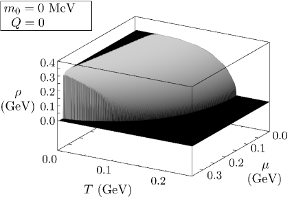
Figure 12: Pion condensate in the chiral limit for neutral matter as a function of quark chemical potential $\mu$ and temperature $T$.

5.2 Physical point

Again the two possible solutions of the gap equations are 1) $\rho=0$ and 2) $\rho\neq 0$. It turns out that the only solution is $\rho=0$, i.e. there is no charged pion condensate at the physical point. In other words, the isospin chemical potential $\mu_{I}=\mu_{Q}$ is always smaller than the pion mass.

This is in accordance with the results of a recent study by Abuki et al [43], where they investigated pion condensation in neutral matter as a function of the pion mass from the chiral limit all the way to the physical value of $139$ MeV. They found a tiny window of pion condensation for pion masses below approximately 10 KeV. Thus pion condensation is very sensitive to the explicit chiral symmetry breaking due to a finite quark mass $m_{0}$.

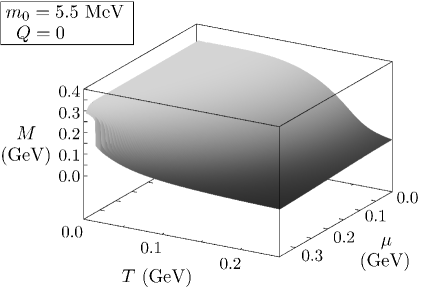
Figure 13: Chiral condensate at the physical point for neutral matter as a function of temperature $T$ and quark chemical potential $\mu$

In Fig. 13, we show the chiral condensate for neutral matter as a function of temperature and quark chemical potential. The chiral condensate decreases with increasing $\mu$ and $T$, but never vanishes.

6 Summary

In this paper, we have calculated the phase diagram of the two-flavour NJL model as a function of the quark and the isospin chemical potential, and the temperature in the chiral limit and at the physical point. In the chiral limit, we have reproduced the results in Refs. [38, 39] at $T=0$ and generalized them to finite temperature. At the physical point, we get similar results for the phase structure as those obtained in Ref. [37]. The qualitative differences are due to different interaction terms in the Lagrangian and a different way of regulating the loop diagrams in the gap equations.

It is natural to ask what happens at larger values of isospin chemical potential. We have extended our calculations of Sec. 3 for $\mu=m_{0}=0$ up to $\delta\mu\approx 900$ MeV. These calculations seem to indicate that there is a phase transition from a pion condensed phase to a chirally symmetric phase. For zero temperature, this transition is located at $\delta\mu\sim 880$ MeV. However, this result should not be trusted since the UV cutoff is $651$ MeV. In fact, there are reasons to believe that there is no phase transition as one increases $\delta\mu$. On general grounds, one can show that there is a nonzero condensate of the form $\langle\bar{d}\gamma_{5}u\rangle$ for larger values of $\mu_{I}$ [25]. Thus one expects a BEC-BCS type of crossover as the quarks bound in the pions become weakly bound due to the fact that the QCD running coupling becomes weaker with increasing chemical potential $\mu_{I}$.

Our main result comes from imposing the constraints of electric charge neutrality and weak equilibrium. In Ref. [39], the authors calculate the phases of neutral matter with another set of parameters at zero temperature. Using an ultraviolet cutoff of $600$ MeV, a coupling constant $G=6.82$ (GeV)^-2, and a constituent quark mass of $400$ MeV, their numerical analysis shows that the phase structure differs from the first set of parameters. At $T=0$, there is in this case no phase with a pion condensate, but a phase transition directly from a phase of broken chiral symmetry to a chirally symmetric phase at a critical quark chemical potential of $\mu_{c}=386.2$ MeV. This seems to indicate that the window for pion condensation at $T=0$ that can be seen in Fig. 12 is not a robust result.

We have seen that the charge neutrality constraint changes the phase diagram since it rules out charged pion condensation at the physical point. This is true for pion masses larger than approximately 10 KeV [43]. However, in the presence of a dense neutrino gas, pion condensation again becomes a possibility even with realistic values of $m_{\pi}$, as shown in Ref. [46]. In nature this situation arises in supernova explosions and possibly at the early stages of the evolution of a neutron star. It does not arise in stable matter such as we have considered here, because the weakly interacting neutrinos will have had time to leave the system.

A natural next step would be to investigate the competition between pion and kaon condensation in neutral matter using a three-flavour NJL model at finite temperature and finite quark chemical potentials $\mu_{u}$, $\mu_{d}$, and $\mu_{s}$. Calculations without the neutrality constraint have already been done by Barducci et al [69].

References

References

- [1] F. Wilczek, Lectures given at 9th CRM Summer School: Theoretical Physics at the End of the 20th Century, Banff, Alberta, Canada, 27 Jun - 10 Jul 1999. Published in *Banff 1999, Theoretical physics at the end of the twentieth century* 567. e-Print: hep-ph/0003183.
- [2] K.Rajagopal and F. Wilczek, Chapter 35 in the Festschrift in honour of B.L. Ioffe, “At the Frontier of Particle Physics / Handbook of QCD”, M. Shifman, ed., (World Scientific). In *Shifman, M. (ed.): At the frontier of particle physics, vol. 3* 2061-2151. e-Print: hep-ph/0011333.
- [3] D. H. Rischke, Prog. Part. Nucl. Phys. 52, 197 (2004).
- [4] M. A. Stephanov, PoS LAT2006, 024 (2006).
- [5] L. McLerran and R. D. Pisarski, Nucl. Phys. A796, 83 (2007).
- [6] M. G. Alford, A. Schmitt, and K. Rajagopal, Rev. Mod. Phys. 80, 1455 (2008).
- [7] P. Braun-Munzinger and J. Wambach, Rev. Mod. Phys. 81, 1031 (2009).
- [8] D. T. Son and M. A. Stephanov, Phys. Rev. D 61, 074012 (2000); Erratum-ibid. 62, 059902 (2000).
- [9] P. F. Bedaque and T. Schafer, Nucl. Phys. A697, 802 (2002).
- [10] D. B. Kaplan and S. Reddy, Phys. Rev. D 65, 054042 (2002).
- [11] T. Schafer, Phys. Rev. D 65, 094033 (2002).
- [12] M. Buballa, Phys. Lett. B609, 57 (2005).
- [13] M. M. Forbes, Phys. Rev. D72, 094032 (2005).
- [14] D. Ebert and K. G. Klimenko, Phys. Rev. D 75, 045005 (2007).
- [15] M. Ruggieri, JHEP 0707, 031 (2007).
- [16] D. Ebert and K.G. Klimenko, arXiv:0809.5254.
- [17] V. Kleinhaus, M. Buballa, D. Nickel, and M. Oertel, Phys. Rev. D 76, 074024 (2007).
- [18] H. J. Warringa, hep-ph/0606063.
- [19] M. G. Alford, M. Braby, and A. Schmitt, J. Phys. G: nucl. Part. Phys. 35, 025002 (2008).
- [20] D. Ebert, , K. G. Klimenko, and V. L. Yudichev, Eur. Phys. J. C53, 65 (2008).
- [21] J. O. Andersen and L. E. Leganger, Nucl. Phys. A828, 360 (2009).
- [22] T. H. Phat, N. V. Long, N. T. Anh, and, L V Hoa, Phys. Rev. D 78, 105016 (2008).
- [23] J. B. Kogut and D. K. Sinclair, Phys. Rev. D 64 034508 (2002); ibid D 66 34505 (2002); ibid D 70, 094501 (2004).
- [24] S. Gupta, hep-lat/0202005.
- [25] P. de Forcrand, M. A. Stephanov, U. Wenger, PoS LAT2007, (237) 2007.
- [26] D. T. Son and M. Stephanov, Phys. Rev. Lett. 86, 592 (2001).
- [27] K. Splittorff, D. T. Son and M. Stephanov, Phys. Rev. D 64 016003 (2001).
- [28] M. Loewe and C. Villavicencio, Phys. Rev. D 67, 074034 (2003); ibid D 70, 074005 (2004); ibid D 71, 094001 (2005).
- [29] A. Barducci, R. Casalbuoni, G. Pettini, and L. Ravagli, Phys. Lett. B564, 217 (2003).
- [30] A. Jakovac, A. Patkos, Zs. Szep, and P. Szepfalusy, Phys. Lett. B582, 179 (2004).
- [31] J. I. Kapusta, Phys. Rev. D 24, 426, (1981).
- [32] H. E. Haber and H. A. Weldon, Phys. Rev. D 25, 502, (1982).
- [33] L. He, M. Jin, and P. Zhuang, Phys. Rev. D 71, 116001 (2005).
- [34] J. O. Andersen, Phys. Rev. D 75, 065011 (2007).
- [35] J. O. Andersen and T. Brauner, Phys. Rev. D 78, 014030 (2008).
- [36] S. Shu and J.-R. Li, J.Phys. G34, 2727 (2007).
- [37] A. Barducci, R. Casalbuoni, G. Pettini, and L. Ravagli, Phys. Rev. D 69, 096004 (2004).
- [38] D. Ebert and K.G. Klimenko, J. Phys. G Nucl. Part. Phys. 32 599 (2006).
- [39] D. Ebert and K.G. Klimenko, Eur. Phys. J. C 46, 771 (2006).
- [40] S. Lawley, W. Bentz, and A. W. Thomas, Phys. Lett. B632, 495 (2006).
- [41] L. He, M. Jin, and P. Zhuang, Phys.Rev. D 71, 116001 (2005).
- [42] X. Hao and P. Zhuang, Phys.Lett. B652, 275 (2007).
- [43] H. Abuki, R. Anglani, R. Gatto, M. Pellicoro, and M. Ruggieri, Phys. Rev. D 79, 034032 (2009).
- [44] S. Mukherjee and, M. G. Mustapha, and R. Ray, Phys Rev. D 75, 094015 (2006).
- [45] H. Abuki, M. Ciminale, R. Gatto, N.D. Ippolito, G. Nardulli, and M. Ruggieri, Phys. Rev. D 78, 014002 (2008); M. Ruggieri, Prog. Theor. Phys. Suppl.174, 60 (2008).
- [46] H. Abuki, T. Brauner and H. J. Warringa, Eur. Phys. J. C64, 123 (2009).
- [47] M. Alford and K. Rajagopal, JHEP, 0206, 031 (2002).
- [48] I. A. Shovkovy, Found. Phys. 35, 1309 (2005).
- [49] D. D. Dietrich and D. H. Rischke, Prog. Part. Nucl. Phys. 53, 305 (2004).
- [50] M. Buballa and I. A. Shovkovy, Phys. Rev. D 72, ’097501 (2005).
- [51] D. Blaschke, S. Fredriksson, H. Grigorian, A.M. Oztas, and F. Sandin, Phys. Rev. D 72, 065020 (2005).
- [52] M. Huang and I. A. Shovkovy, Nucl. Phys. A729, 835 (2003); M. Huang, Int. J. Mod. Phys. E 14, 675 (2005).
- [53] M. Buballa, Phys. Rept. 407, 205 (2005).
- [54] G. ’t Hooft, Phys. Rept.142, 357 (1986).
- [55] M. Kobayashi and T. Maskawa, Prog. Theor. Phys. 44, 1422 (1970).
- [56] G. ’t Hooft, Phys Rev. Lett. 37, 8 (1976).
- [57] F. Dautry and E. M. Nyman, Nucl. Phys. A319, 323 (1979).
- [58] W. Broniowski and M. Kutschera, Phys. Lett. B242, 133 (1990).
- [59] M. Sadzikowski and W. Broniowski, Phys. Lett. B488, 63 (2000).
- [60] M. Sadzikowski, Phys. Lett. B553, 45 (2003).
- [61] M. Sadzikowski, Phys. Lett. B642, 238 (2006).
- [62] T. L. Partyka and M. Sadzikowski, J. Phys. G 36, 025004 (2008).
- [63] V. A. Miransky and I. A. Shovkovy, Phys. Rev. Lett. 88, 111601 (2002).
- [64] M. Alford and Q. Wang, J. Phys. G: Nucl. Part. Phys. 31, 719 (2005).
- [65] M. Alford, K. Rajagopal, and F. Wilczek, Phys. Lett. B422, 247, (1998).
- [66] H. B. Nielsen and S. Chadha, Nucl. Phys. B105, 445 (1976).
- [67] T. Schäfer, D. T. Son, M. A. Stephanov, D. Toublan, and J. J. M. Verbaarschot, Phys. Lett. B522, 67 (2001).
- [68] T. Brauner, Phys. Rev. D 72, 076002 (2005); PhD Thesis, Nuclear Physics Institute, Prague (2006), hep-ph/0606300.
- [69] A. Barducci, R. Casalbuoni, G. Pettini, and L. Ravagli, Phys. Rev. D 71, 016011 (2005).