The diquark and elastic pion-proton scattering at high energies

Abstract

Small momentum transfer elastic pion-proton cross-section at high energies is calculated assuming the proton is composed of two constituents, a quark and a diquark. We find that it is possible to fit very precisely the data when (i) the pion acts as a single entity (no constituent quark structure) and (ii) the diquark is rather large, comparable to the size of the proton.

1 Introduction

In this note we study the quark correlations inside the nucleon - forming a diquark [1] - in the context of elastic pion-proton scattering at low momentum transfer.

The interest in this process is a consequence of Ref. [2] where the elastic proton-proton scattering, assuming the proton is composed of quark and diquark, was discussed. We found that (i) it was possible to fit very precisely the ISR elastic $pp$ data [3] even up to $-t\approx 3$ GeV² and (ii) the diquark turned out to be rather large, comparable to the size of the proton. Moreover, we found that the quark-diquark model of the nucleon in the wounded [4] constituent model [5] allows to explain very well the RHIC data [6] on particle production in the central rapidity region.

Given above arguments, it is interesting to explore the model for another process. The natural one is elastic pion-proton scattering. Following [2] we consider the proton to be composed of two constituents - a quark and a diquark. As far as the pion is concerned we consider two cases. The first one treats the pion as an object composed of two constituent quarks, the second one treats the pion as a single object i.e. an object without constituent quark structure.

For both cases we evaluate the inelastic pion-proton cross-section, $\sigma(b)$, at a given impact parameter $b$. Then, from the unitarity condition we obtain the elastic amplitude

$$t_{el}(b)=1-\sqrt{1-\sigma(b)},$$ (1)

and consequently the elastic amplitude in momentum transfer representation:

$$T(\Delta)=\int t_{el}(b)e^{i\vec{\Delta}\cdot\vec{b}}d^{2}b.$$ (2)

With this normalization one can evaluate the total cross section:

$$\sigma_{tot}=2T(0),$$ (3)

and elastic differential cross section ($t\simeq-|\Delta|^{2}$):

$$\frac{d\sigma}{dt}=\frac{1}{4\pi}|T(\Delta)|^{2}.$$ (4)

Our strategy is to adjust the parameters of the model so that it fits best the data for elastic pion-proton cross-section. In this way the model can provide some information on the details of proton and pion structure at small momentum transfer.

2 Pion as a quark-quark system

We follow closely the method presented in [2] where the elastic and inelastic proton-proton collision was studied. Consequently, the inelastic pion-proton cross-section at a fixed impact parameter $b$, $\sigma(b)$, is given by:

$$\sigma(b)=\int d^{2}s_{q}d^{2}s_{d}d^{2}s_{q1}d^{2}s_{q2}D_{p}(s_{q},s_{d})D_{\pi}(s_{q1},s_{q2})\sigma(s_{q},s_{d};s_{q1},s_{q2};b),$$ (5)

where $D_{p}(s_{q},s_{d})$ and $D_{\pi}(s_{q1},s_{q2})$ denote the distribution of quark ($s_{q}$) and diquark ($s_{d}$) inside the proton and the distribution of quarks ($s_{q1}$,$s_{q2}$) inside the pion, respectively. $\sigma(s_{q},s_{d};s_{q1},s_{q2};b)$ is the probability of inelastic interaction at fixed impact parameter $b$ and frozen transverse positions of all constituents. The schematic view of this process is shown in Fig. 1.

Using the Glauber [7] and Czyz-Maximon [8] expansions we have:

$$1-\sigma(s_{q},s_{d};s_{q1},s_{q2};b) =[1-\sigma_{qq}(b+s_{q1}-s_{q})][1-\sigma_{qq}(b+s_{q2}-s_{q})]\times$$

$$\times [1-\sigma_{qd}(b+s_{q1}-s_{d})][1-\sigma_{qd}(b+s_{q2}-s_{d})],$$ (6)

where $\sigma_{ab}(s)$ ($ab$ denotes $qq$ or $qd$) are inelastic differential cross-sections of the constituents.

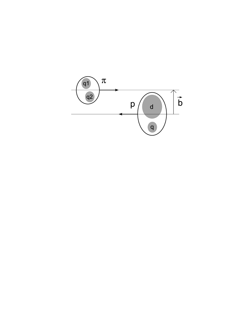
Figure 1: Pion-proton scattering in the quark-diquark model. Pion as a quark-quark system.

Following [2] we parametrize $\sigma_{ab}(s)$ using simple Gaussian forms:

$$\sigma_{ab}(s)=A_{ab}e^{-s^{2}/R_{ab}^{2}}.$$ (7)

We constrain the radii $R_{ab}$ by the condition: $R_{ab}^{2}=R_{a}^{2}+R_{b}^{2}$ where $R_{a}$ denotes the quark or diquark’s radius.

From (7) we obtain the total inelastic cross sections: $\sigma_{ab}=\pi A_{ab}R_{ab}^{2}$. Following [2] we assume that the ratios of cross-sections satisfy the condition: $\sigma_{qd}/\sigma_{qq}=2$, what allows to evaluate $A_{qd}$ in term of $A_{qq}$.

For the distribution of the constituents inside the proton we take a Gaussian with radius $R$:

$$D_{p}(s_{q},s_{d})=\frac{1+\lambda^{2}}{\pi R^{2}}e^{-(s_{q}^{2}+s_{d}^{2})/R^{2}}\delta^{2}(s_{d}+\lambda s_{q}),$$ (8)

where the parameter $\lambda$ has the physical meaning of the ratio of the quark and diquark masses $\lambda=m_{q}/m_{d}$ (the delta function guarantees that the center-of-mass of the system moves along the straight line). One expects $1/2\leq\lambda\leq 1$.

For the distribution of quarks inside the pion we take a Gaussian with radius $d$:

$$D_{\pi}(s_{q1},s_{q2})=\frac{1}{\pi d^{2}}e^{-(s_{q1}^{2}+s_{q2}^{2})/2d^{2}}\delta^{2}(s_{q1}+s_{q2}).$$ (9)

It allows to define the effective pion radius $R_{\pi}$:

$$R_{\pi}^{2}=d^{2}+R_{q}^{2}.$$ (10)

Now the calculation of $\sigma(b)$, given by (5), reduces to straightforward Gaussian integrations. The relevant formula is given in the Appendix. Introducing this result into the general formulae given in Section $1$ one can evaluate the total and elastic differential pion-proton cross-sections.

Our strategy is to adjust the parameters of the model so that it fits the data best. We have analyzed the data for elastic $\pi^{+}p$ scattering at two incident momenta $p_{lab}=$ $100$ GeV and $200$ GeV [9]. An example of our calculation is shown in Fig. 2, where the differential cross section $d\sigma/dt$ at $p_{lab}=200$ GeV, evaluated from the model, is compared with data [9].

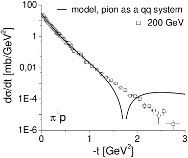
Figure 2: The model compared to data [9] on differential cross section for elastic $\pi^{+}p$ scattering at $p_{lab}=200$ GeV (not all points plotted, for clarity). Pion as a quark-quark system.

From Fig. 2 one sees that it is possible to fit very precisely the data up to $-t\approx 1$ GeV². However, the model, with the pion as a two-quark system, predicts the diffractive minimum which is not seen in the data. In the next section we show that assuming the pion to be a single entity (no constituent quark structure) we are able to remove this problem.

The relevant values of the parameters are given in Table 1.

$p_{lab}$ [GeV]	$R_{q}$ [fm]	$R_{d}$ [fm]	$R$ [fm]	$R_{\pi}$ [fm]	$A_{qq}$
$200$	0.26	0.82	0.28	0.44	1

Table 1: The parameters of the model at the incident momentum $p_{lab}=200$ GeV. Pion as a quark-quark system.

It is intriguing to notice that the values of the most interesting parameters, $R_{q}$ and $R_{d}$, are not far from those obtained in [2] were elastic $pp$ scattering was studied in similar approach. Again we observe that the diquark is rather large.

3 Pion as a single entity

In the present section we assume that the pion interacts as a single entity i.e. the pion has no constituent quark structure. The schematic view of the pion-proton scattering in this approach is shown in Fig. 3.

The inelastic pion-proton cross-section $\sigma(b)$ at a fixed impact parameter $b$ reads:

$$\sigma(b)=\int d^{2}s_{q}d^{2}s_{d}D_{p}(s_{q},s_{d})\sigma(s_{q},s_{d};b),$$ (11)

with $D_{p}(s_{q},s_{d})$ given by (8) and $\sigma(s_{q},s_{d};b)$ expressed by:

$$1-\sigma(s_{q},s_{d};b)=[1-\sigma_{q\pi}(b-s_{q})][1-\sigma_{d\pi}(b-s_{d})].$$ (12)

In analogy to the previous approach the inelastic differential quark-pion, $\sigma_{q\pi}(s)$, and diquark-pion, $\sigma_{d\pi}(s)$, cross sections are parametrized using simple Gaussian:

$$\sigma_{a\pi}(s)=A_{a\pi}e^{-s^{2}/R_{a\pi}^{2}}.$$ (13)

In this case we constrain the radii $R_{a\pi}$ by the condition: $R_{a\pi}^{2}=R_{a}^{2}+R_{\pi}^{2}$ where $R_{a}$ denotes the quark or diquark’s radius and $R_{\pi}$ denotes the pion’s radius.

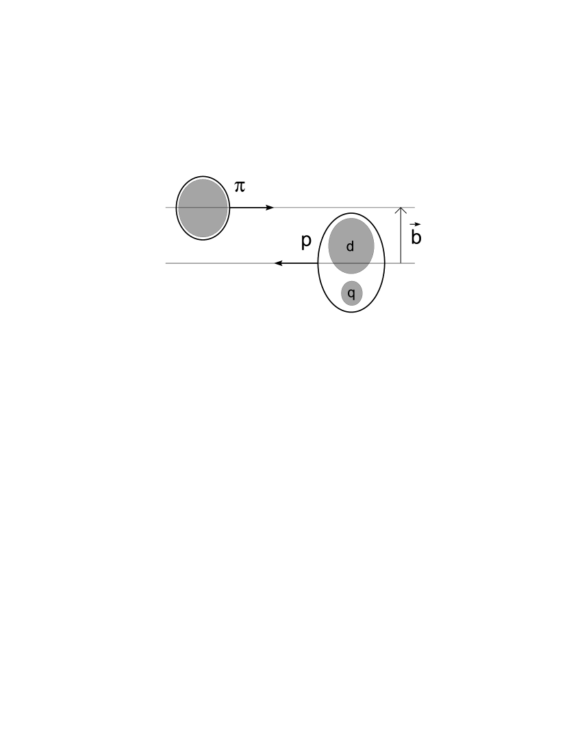
Figure 3: Pion-proton scattering with the pion as a single entity.

This gives:

$$\sigma(b) =\frac{A_{q\pi}x}{x+r}e^{-b^{2}/(x+r)}+\frac{A_{d\pi}y}{y+\lambda^{2}r}e^{-b^{2}/(y+\lambda^{2}r)}$$ (14)

$$-\frac{A_{q\pi}A_{d\pi}xy}{xy+yr+\lambda^{2}xr}e^{-b^{2}\tfrac{x+y+(1+\lambda)^{2}r}{xy+yr+\lambda^{2}xr}},$$

where $x=R_{q}^{2}+R_{\pi}^{2},$ $y=R_{d}^{2}+R_{\pi}^{2}$ and $r=R^{2}/(1+\lambda^{2})$. Introducing this result into the general formulae given in Section $1$ one can evaluate the total and elastic differential pion-proton cross-sections.

From (13) we deduce the total inelastic cross sections: $\sigma_{a\pi}=\pi A_{a\pi}R_{a\pi}^{2}$. As before we demand that the ratios of cross-sections satisfy the condition: $\sigma_{d\pi}/\sigma_{q\pi}=2$, what allows to evaluate $A_{d\pi}$ in term of $A_{q\pi}$.

It turns out that the model in this form works very well indeed i.e. it is possible to fit very precisely the data even up to $-t\approx 3$ GeV². We have analyzed the data at two incident momenta of $100$ and $200$ GeV [9]. The results of our calculations are shown in Fig. 4.

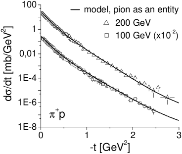
Figure 4: Pion acts as a single entity. The model compared to data [9] (not all points plotted, for clarity) on differential cross section for elastic $\pi^{+}p$ scattering at $p_{lab}=100$ GeV (rescaled by a factor $10^{-2}$) and $200$ GeV.

The relevant values of the parameters are given in Table 2. Again the most interesting observation is the large size of the diquark, comparable to the size of the proton.

$p_{lab}$ [GeV]	$R_{q}$ [fm]	$R_{d}$ [fm]	$R$ [fm]	$R_{\pi}$ [fm]	$A_{q\pi}$
$100$	0.25	0.79	0.28	0.50	0.80
$200$	0.25	0.79	0.28	0.52	0.75

Table 2: The parameters of the model at two incident momenta $p_{lab}=100$ GeV and $200$ GeV. Pion acts as a single entity.

4 Discussion and conclusions

In conclusion, it was shown that the constituent quark-diquark structure of the proton can account very well for the data on elastic $\pi^{+}p$ scattering. The detailed confrontation with data allows to determine the parameters characterizing the proton and pion structure. We confirm the large size of the diquark, while the pion seems to interact as a single entity i.e. without constituent quark structure.

Several comments are in order.

(a) We compared the model only to elastic $\pi^{+}p$ scattering data, however, there is no statistically significant difference between $\pi^{+}p$ and $\pi^{-}p$ data [9] at any $t$ value (at least up to $-t\approx 3$ GeV²).

(b) The pion seems to interact as a single entity. It suggests that during pion-nucleus collision the pion produces the same number of particles no matter how many inelastic collisions it undergoes.

Acknowledgements

We thank Andrzej Bialas for suggesting this investigation and illuminating discussions. Discussions with Stephane Munier, Robert Peschanski, Michal Praszalowicz and Samuel Wallon are also highly appreciated.

5 Appendix

The problem is to calculate the following integral:

$$\frac{r_{1}r_{2}}{\pi^{2}}\int d^{2}sd^{2}s^{\prime}e^{-r_{1}s^{2}}e^{-r_{2}s^{\prime 2}}e^{-y_{1}(b+\lambda s-s^{\prime})^{2}}e^{-y_{2}(b+\lambda s+s^{\prime})^{2}}\times$$ (15)

$$\times e^{-x_{1}(b-s-s^{\prime})^{2}}e^{-x_{2}(b-s+s^{\prime})^{2}}=\frac{r_{1}r_{2}}{\Omega}e^{-b^{2}\Gamma/\Omega},$$

where:

$$\Gamma =(1+\lambda)^{2}\left[4x_{1}x_{2}(y_{1}+y_{2})+4y_{1}y_{2}(x_{1}+x_{2})+r_{2}(x_{1}+x_{2})(y_{1}+y_{2})\right]$$

$$+4r_{1}(x_{1}+y_{1})(x_{2}+y_{2})+r_{1}r_{2}(x_{1}+x_{2}+y_{1}+y_{2}),$$ (16)

$$\Omega =(1-\lambda)^{2}(x_{1}y_{2}+x_{2}y_{1})+(1+\lambda)^{2}(x_{1}y_{1}+x_{2}y_{2})+\lambda^{2}[r_{2}(y_{1}+y_{2})+4y_{1}y_{2}]$$

$$+r_{1}(x_{1}+x_{2}+y_{1}+y_{2}+r_{2})+r_{2}(x_{1}+x_{2})+4x_{1}x_{2}.$$ (17)

Other needed integrals can be obtained by putting some of the $x_{1},$ $x_{2},$ $y_{1}$ or $y_{2}=0$.

References

- [1] See, e.g., R. L. Jaffe, Phys. Rept. 409 (2005) 1; C. Alexandrou, Ph. de Forcrand, B. Lucini, hep-lat/0609004; M. Cristoforetti, P. Faccioli, G. Ripka, M. Traini, Phys. Rev. D71 (2005) 114010.
- [2] A. Bialas, A. Bzdak, hep-ph/0612038.
- [3] E. Nagy et al., Nucl. Phys. B150 (1979) 221; N. Amos et al., Nucl. Phys. B262 (1985) 689; A. Breakstone et al., Nucl. Phys. B248 (1984) 253; A. Bohm et al., Phys. Lett. B49 (1974) 491.
- [4] A. Bialas, M. Bleszynski, W. Czyz, Nucl. Phys. B111 (1976) 461.
- [5] A. Bialas, A. Bzdak, nucl-th/0611021.
- [6] B. B. Back et al., Phys. Rev. C65 (2002) 061901; Phys. Rev. C70 (2004) 021902; Phys. Rev. C72 (2005) 031901; Phys. Rev. C74 (2006) 021901.
- [7] R. J. Glauber, Lectures in Theoretical Physics, Vol. 1. Interscience, New York 1959.
- [8] W. Czyz, L. C. Maximon, Ann. of Phys. 52 (1969) 59.
- [9] A. S. Carroll et al., Phys. Rev. Lett. 33 (1974) 932; A. Schiz et al., Phys. Rev. D24 (1981) 26; C. W. Akerlof et al., Phys. Rev. D14 (1976) 2864; R. L. Cool et al., Phys. Rev. D24 (1981) 2821; R. Rubinstein et al., Phys. Rev. D30 (1984) 1413.