Expectations on $B\to\left(K^{*}_{0}(1430),K^{*}_{2}(1430)\right)\phi$ decays

Abstract

As the annihilation contributions play important roles in solving the puzzle of the small longitudinal polarizations in $B\to K^{*}\phi$ decays, we examine the similar effects in the decays of $B\to K^{*}_{0,2}(1430)\phi$. For the calculations on the annihilated contributions, we adopt that the form factors in $B\to K^{(*)}\phi$ decays are parameters determined by the observed branching ratios (BRs), polarization fractions (PFs) and relative angles in experiments and we connect the parameters between $B\to K^{*}_{0(2)}\phi$ and $B\to K^{(*)}\phi$ by the ansatz of correlating $\langle K^{*}_{n}(1430)\phi|(V-A)_{\mu}|0\rangle$ to $\langle K^{(*)}\phi|(V-A)_{\mu}|0\rangle$. We find that the BR of $B_{d}\to K^{*0}_{0}(1430)\phi$ is $(3.69\pm 0.47)\times 10^{-6}$. By using the transition form factors of $B\to K^{*}_{2}(1430)$ in the light-front quark model (LFQM) and the 2nd version of Isgur-Scora-Grinstein-Wise (ISGW2), we show that BR of $B_{d}\to K^{*0}_{2}(1430)\phi$ is a broad allowed value and $(1.70\pm 0.80)\times 10^{-6}$, respectively. In terms of the recent BABAR’s observations on BRs and PFs in $B_{d}\to K^{*0}_{2}(1430)\phi$, the results in the LFQM are found to be more favorable. In addition, due to the annihilation contributions to $B\to K^{*}_{2}\phi$ and $B\to K^{*}\phi$ being opposite in sign, we demonstrate that the longitudinal polarization of $B_{d}\to K^{*0}_{2}(1430)\phi$ is always $O(1)$ with or without including the annihilation contributions.

I Introduction

Since the transverse decay amplitudes of vector meson productions in $B$ decays are associated with their masses, by naive estimations, the longitudinal polarization (LP) of $B$ decaying into two light vector mesons is close to unity. The expectation is confirmed by BELLE belle1 and BABAR babar1-1 ; babar1-2 in $B\to\rho(\omega)\rho$ decays, in which the longitudinal parts occupy over $88\%$. Furthermore, the LPs could be small if the final states include heavy vector mesons. The conjecture is verified in $B\to J/\Psi K^{*}$ decays belle2 ; babar2 , in which the longitudinal contribution is only about $60\%$. However, the rule for the small LPs seems to be violated in $B\to\phi K^{*}$ decays. From the measurements of BELLE belle3 and BABAR babar1-1 ; babar3 , it is quite clear that the LPs in $B\to K^{*}\phi$ are only around $50\%$. To solve the unexpected observations, many mechanisms have been proposed, such as those with new QCD effects Kagan ; QCD ; Chen ; Beneke as well as extensions of the standard model (SM) newphys ; CG_PRD71 .

Recently, the BABAR Collaboration has observed the branching ratios (BRs) and polarization fractions (PFs) for the decays of $B_{d}\to K^{*0}_{0,2}(1430)\phi$ babar4 , given by

$$BR(B_{d}\to K^{*0}_{2}(1430)\phi) = (7.8\pm 1.1\pm 0.6)\times 10^{-6}\,,$$

$$R_{L}(B_{d}\to K^{*0}_{2}(1430) = 0.853^{+0.061}_{-0.069}\pm 0.036\,,$$

$$R_{\perp}(B_{d}\to K^{*0}_{2}(1430) = 0.045^{+0.049}_{-0.040}\pm 0.013\,,$$

$$BR(B_{d}\to K^{*0}_{0}(1430)\phi) = (4.6\pm 0.7\pm 0.6)\times 10^{-6}\,.$$ (1)

By the observations, it seems that the LP of the p-wave tensor-meson production is much larger than those of the s-wave vector mesons in $B$ decays. To find out whether the data are just the statistical fluctuation or the correct tendency for the behavior of the p-wave productions in $B$ decays, it is important to study the phenomena from theoretical viewpoint.

It is known that the annihilation contributions play important roles in the PFs of $B\to K^{*}\phi$ decays Kagan ; Chen ; Beneke . As the corresponding time-like form factors are more uncertain than those of the transition form factors, we first adopt that the form factors of the annihilation contributions on $B\to K^{*}\phi$ are parameters fixed by the data in $B\to K^{*}\phi$ and then connect them to those in $B_{d}\to K^{*0}_{2}(1430)\phi$. To have more illustrating examples, we also examine the decays of $B\to K^{*}_{0}(1430)\phi$ simultaneously.

The paper is organized as follows. In Sec. II, we carry out a general study on the decay amplitudes and hadronic matrix elements. We present our numerical analysis in Sec. III. Our conclusions are presented in Sec. IV.

II Decay amplitudes and hadronic matrix elements

It is known that the effective interactions for the decays of $B\to K^{*}_{n}(1430)\phi\ (n=0,2)$ are described by $b\to sq\bar{q}$, which are the same as $B\to K^{(*)}\phi$, given by BBL

$$H_{{\rm eff}}={\frac{G_{F}}{\sqrt{2}}}\sum_{q=u,c}V_{q}\left[C_{1}(\mu)O_{1}^{(q)}(\mu)+C_{2}(\mu)O_{2}^{(q)}(\mu)+\sum_{i=3}^{10}C_{i}(\mu)O_{i}(\mu)\right]\;,$$ (2)

where $V_{q}=V_{qs}^{*}V_{qb}$ are the Cabibbo-Kobayashi-Maskawa (CKM) matrix elements CKM and the operators $O_{1}$-$O_{10}$ are defined as

$$O_{1}^{(q)}=(\bar{s}_{\alpha}q_{\beta})_{V-A}(\bar{q}_{\beta}b_{\alpha})_{V-A}\;,\;\;\;\;\;\;\;\;O_{2}^{(q)}=(\bar{s}_{\alpha}q_{\alpha})_{V-A}(\bar{q}_{\beta}b_{\beta})_{V-A}\;,$$

$$O_{3}=(\bar{s}_{\alpha}b_{\alpha})_{V-A}\sum_{q}(\bar{q}_{\beta}q_{\beta})_{V-A}\;,\;\;\;\;O_{4}=(\bar{s}_{\alpha}b_{\beta})_{V-A}\sum_{q}(\bar{q}_{\beta}q_{\alpha})_{V-A}\;,$$

$$O_{5}=(\bar{s}_{\alpha}b_{\alpha})_{V-A}\sum_{q}(\bar{q}_{\beta}q_{\beta})_{V+A}\;,\;\;\;\;O_{6}=(\bar{s}_{\alpha}b_{\beta})_{V-A}\sum_{q}(\bar{q}_{\beta}q_{\alpha})_{V+A}\;,$$

$$O_{7}=\frac{3}{2}(\bar{s}_{\alpha}b_{\alpha})_{V-A}\sum_{q}e_{q}(\bar{q}_{\beta}q_{\beta})_{V+A}\;,\;\;O_{8}=\frac{3}{2}(\bar{s}_{\alpha}b_{\beta})_{V-A}\sum_{q}e_{q}(\bar{q}_{\beta}q_{\alpha})_{V+A}\;,$$

$$O_{9}=\frac{3}{2}(\bar{s}_{\alpha}b_{\alpha})_{V-A}\sum_{q}e_{q}(\bar{q}_{\beta}q_{\beta})_{V-A}\;,\;\;O_{10}=\frac{3}{2}(\bar{s}_{\alpha}b_{\beta})_{V-A}\sum_{q}e_{q}(\bar{q}_{\beta}q_{\alpha})_{V-A}\;,$$ (3)

with $\alpha$ and $\beta$ being the color indices and $C_{1}$-$C_{10}$ the corresponding Wilson coefficients (WCs). In Eq. (2), $O_{1}$-$O_{2}$ are from the tree level of weak interactions, $O_{3}$-$O_{6}$ are the so-called gluon penguin operators and $O_{7}$-$O_{10}$ are the electroweak penguin operators. Using the unitarity condition, the CKM matrix elements for the penguin operators $O_{3}$-$O_{10}$ can also be expressed by $V_{u}+V_{c}=-V_{t}$. Besides the weak effective interactions, to study exclusive two-body decays, we should know how to calculate the transition matrix elements such as $\langle M_{1}M_{2}|H_{\rm eff}|B\rangle$, where nonperturbative effects dominate the uncertainties. By taking the heavy quark limit, we consider that the productions of light mesons satisfy the assumption of color transparency Bjorken , i.e., the final state interactions are subleading effects and negligible. Hence, the decays of $B\to K^{*}_{n}(1430)\phi$ could be treated as short-distance dominant processes. As the wave functions of p-wave states are quite uncertain, unlike those of s-wave states which are known at least in the leading twist-2 and twist-3 WF_QCD , in our calculations we will employ the generalized factorization assumption GFA1 ; GFA2 , in which the factorized parts are regarded as the leading effects and the nonfactorized effects are lumped and characterized by the effective number of colors, denoted by $N^{\rm eff}_{c}$ BSW .

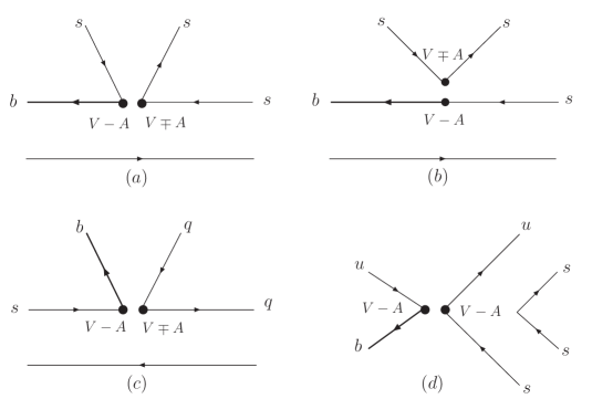
Based on the effective interactions of Eq. (2), the matrix elements $\langle K^{*}_{n}(1430)\phi|H_{\rm eff}|B\rangle$ could be classified by various flavor diagrams displayed in Fig. 1, where (a) and (b) denote the penguin emission topologies, while (c)[(d)] is the penguin [tree] annihilation topology.

Figure 1: Flvaor diagrams for $B\to\left(K^{*}_{0}(1430),\,K^{*}_{2}(1430)\right)\phi$ decays, where (a) and (b) denote the penguin emission topologies, while (c) and (d) are the annihilation topologies for penguin and tree contributions, respectively.

Furthermore, in terms of the flavor diagrams, we can group the effects of Eq. (2) for the transition matrix elements to be

$$X^{(BK^{*}_{n},\phi)} = \langle\phi|(\bar{s}s)_{V\pm A}|0\rangle\,\langle K^{*}_{n}|(\bar{b}s)_{V-A}|B\rangle\,,$$

$$Z^{(B,K^{*}_{n}\phi)}_{1} = \langle K^{*}_{n}\phi|(\bar{q}s)_{V-A}|0\rangle\,\langle 0|(\bar{b}q)_{V-A}|B\rangle\,,$$

$$Z^{(B,K^{*}_{n}\phi)}_{2} = \langle K^{*}_{n}\phi|(\bar{q}s)_{S-P}|0\rangle\,\langle 0|(\bar{b}q)_{S+P}|B\rangle\,,$$ (4)

where $X^{(BK^{*}_{n},\phi)}$ represent the factorized parts of the emission topology and $Z^{(B,K^{*}_{n}\phi)}_{1,2}$ stand for the factorized parts of the annihilation topology. Note that the currents associated with $(S+P)\otimes(S-P)$ in Eq. (4) are from the Fierz transformations of $(V-A)\otimes(V+A)$. From Eqs. (2)-(4), the decay amplitudes for $B\to K^{*}_{n}(1430)\phi$ can be written as

$$A(B_{d}\to K^{*0}_{n}(1430)\phi) = \frac{G_{F}}{\sqrt{2}}\left\{-V_{tb}V^{*}_{ts}\left[\tilde{a}^{(s)}X^{(BK^{*}_{n},\phi)}\right.\right.$$

$$\left.\left.+a^{(s)}_{4}Z^{(B,K^{*}_{n}\phi)}_{1}-2a^{(s)}_{6}Z^{(B,K^{*}_{n}\phi)}_{2}\right]\right\},$$

$$A(B^{+}_{u}\to K^{*+}_{n}(1430)\phi) = \frac{G_{F}}{\sqrt{2}}\left\{V_{us}V_{ub}^{*}a_{1}Z^{(B,K^{*}_{n}\phi)}_{1}-V_{tb}V^{*}_{ts}\left[\tilde{a}^{(s)}X^{(BK^{*}_{n},\phi)}\right.\right.$$ (5)

$$\left.\left.+a^{(u)}_{4}Z^{(B,K^{*}_{n}\phi)}_{1}-2a^{(u)}_{6}Z^{(B,K^{*}_{n}\phi)}_{2}\right]\right\}\,,$$

with $\tilde{a}^{(s)}=a^{(s)}_{3}+a^{(s)}_{4}+a^{(s)}_{5}$. To be more convenient for our analysis, we have redefined the useful WCs by combining the gluon and electroweak penguin contributions to be

$$a_{1} = C^{\rm eff}_{2}+\frac{C^{\rm eff}_{1}}{N^{\rm eff}_{c}},\ \ \ a_{2}=C^{\rm eff}_{1}+\frac{C^{\rm eff}_{2}}{N^{\rm eff}_{c}},\ \ a^{(q)}_{3}=C^{\rm eff}_{3}+\frac{C^{\rm eff}_{4}}{N^{\rm eff}_{c}}+\frac{3}{2}e_{q}\left(C^{\rm eff}_{9}+\frac{C^{\rm eff}_{10}}{N^{\rm eff}_{c}}\right),$$

$$a^{(q)}_{4} = C^{\rm eff}_{4}+\frac{C^{\rm eff}_{3}}{N^{\rm eff}_{c}}+\frac{3}{2}e_{q}\left(C^{\rm eff}_{10}+\frac{C^{\rm eff}_{9}}{N^{\rm eff}_{c}}\right),a^{(q)}_{5}=C^{\rm eff}_{5}+\frac{C^{\rm eff}_{6}}{N^{\rm eff}_{c}}+\frac{3}{2}e_{q}\left(C^{\rm eff}_{7}+\frac{C^{\rm eff}_{8}}{N^{\rm eff}_{c}}\right),$$

$$a^{(q)}_{6} = C^{\rm eff}_{6}+\frac{C^{\rm eff}_{5}}{N^{\rm eff}_{c}}+\frac{3}{2}e_{q}\left(C^{\rm eff}_{8}+\frac{C^{\rm eff}_{7}}{N^{\rm eff}_{c}}\right),$$ (6)

where the effective WCs of $C^{\rm eff}_{i}$ contain vertex corrections for smearing the $\mu$-scale dependences in the transition matrix elements GFA2 and the effective color number of $N^{\rm eff}_{c}$ is a variable, which may not be equal to $3$ GFA1 ; GFA2 ; BSW .

The hadronic matrix elements defined in Eq. (4) are the essential quantities that we have to deal with in the two-body exclusive B decays. In the following discussions, we analyze the quantities $X^{BK^{*}_{n},\phi}$, $Z^{B,K^{*}_{n}\phi}_{1}$ and $Z^{B,K^{*}_{n}\phi}_{2}$ individually. Since the degrees of freedom of $K^{*}_{0}$ are less than those of $K^{*}_{2}$, we start with $B\to K^{*}_{0}(1430)\phi$. As usual, we define the various normal hadronic matrix elements as follows: LF1

$$\langle 0|\bar{b}\gamma^{\mu}\gamma_{5}q|B(p_{B})\rangle = if_{B}p^{\mu}_{B}\,,\ \ \ \langle\phi(q,\,h)|\bar{s}\gamma^{\mu}s|0\rangle=m_{\phi}f_{\phi}\varepsilon^{\mu*}_{\phi}(h)\,,$$

$$\langle K^{*}_{0}(p)|V_{\mu}-A_{\mu}|B(p_{B})\rangle = i\left[\left(P_{\mu}-{m^{2}_{B}-m^{2}_{K^{*}_{0}}\over q^{2}}\,q_{\mu}\right)F_{1}^{BK^{*}_{0}}(q^{2})\right.$$ (7)

$$\left.+{m^{2}_{B}-m^{2}_{K^{*}_{0}}\over q^{2}}\,q_{\mu}\,F_{0}^{BK^{*}_{0}}(q^{2})\right]\,,$$

where $(V_{\mu},A_{\mu})=\bar{b}(\gamma_{\mu},\gamma_{\mu}\gamma_{5})s$, $m_{B,\phi,K^{*}_{0}}$ are the meson masses of $B$, $\phi$ and $K^{*}_{0}$, $P=p_{B}+p$, $q=p_{B}-p$ and $P\cdot q=m^{2}_{B}-m^{2}_{K^{*}_{n}}$. Similarly, the time-like form factors for $\langle K^{*}_{0}\phi|V_{\mu}-A_{\mu}|0\rangle$ could be defined by

$$\langle K^{*}_{0}(p)\phi(q,\varepsilon_{\phi})|V_{\mu}-A_{\mu}|0\rangle = -i\frac{V^{K^{*}_{0}\phi}(q^{2})}{m_{\phi}-m_{K^{*}_{0}}}\epsilon_{\mu\nu\rho\sigma}\varepsilon_{\phi}^{\nu*}Q^{\rho}s^{\sigma}\,,$$ (8)

$$+\left\{2m_{\phi}A^{K^{*}_{0}\phi}_{0}(q^{2})\frac{\varepsilon_{\phi}^{*}\cdot Q}{Q^{2}}Q_{\mu}\right.$$

$$+(m_{\phi}-m_{K^{*}_{0}})A^{K^{*}_{0}\phi}_{1}(q^{2})\Big{(}\varepsilon_{\phi\mu}^{*}-\frac{\varepsilon_{\phi}^{*}\cdot Q}{Q^{2}}Q_{\mu}\Big{)}$$

$$\left.-A^{K^{*}_{0}\phi}_{2}(q^{2})\frac{\varepsilon_{\phi}^{*}\cdot Q}{m_{\phi}-m_{K^{*}_{0}}}\Big{(}s_{\mu}-\frac{s\cdot Q}{Q^{2}}Q_{\mu}\Big{)}\right\}$$

with $Q_{\mu}=(p+q)_{\mu}=p_{B\mu}$ and $s_{\mu}=(p-q)_{\mu}$. In terms of form factors in Eqs. (7) and (8), Eq. (4) could be rewritten as

$$X^{(BK^{*}_{0},\phi)} = i2m_{\phi}f_{\phi}F^{BK^{*}_{0}}_{1}(m^{2}_{\phi})\varepsilon^{*}_{\phi}\cdot p_{B}\,,$$

$$Z^{(B,K^{*}_{0}\phi)}_{1} = -i2m_{\phi}f_{B}A^{K^{*}_{0}\phi}_{0}(m^{2}_{B})\varepsilon^{*}_{\phi}\cdot p_{B}\,,$$

$$Z^{(B,K^{*}_{0}\phi)}_{2} = i2m_{\phi}f_{B}\frac{m^{2}_{B}}{(m_{b}+m_{q})(m_{s}-m_{q})}A^{K^{*}_{0}\phi}_{0}(m^{2}_{B})\varepsilon^{*}_{\phi}\cdot p_{B}\,.$$ (9)

To compare with the s-wave states, we also give the hadronic matrix elements in $B\to K\phi$ as

$$X^{(BK,\phi)} = 2m_{\phi}f_{\phi}F^{BK}_{1}(m^{2}_{\phi})\varepsilon^{*}_{\phi}\cdot p_{B}\,,$$

$$Z^{(B,K\phi)}_{1} = -2m_{\phi}f_{B}A^{K\phi}_{0}(m^{2}_{B})\varepsilon^{*}_{\phi}\cdot p_{B}\,,$$

$$Z^{(B,K\phi)}_{2} = -2m_{\phi}f_{B}\frac{m^{2}_{B}}{(m_{b}+m_{q})(m_{s}+m_{q})}A^{K\phi}_{0}(m^{2}_{B})\varepsilon^{*}_{\phi}\cdot p_{B}\,.$$ (10)

We note that except the factor of $-i$ associated with the p-wave states LF1 , the definitions of the form factors for $\langle K|V_{\mu}-A_{\mu}|B\rangle$ and $\langle K\phi|V_{\mu}-A_{\mu}|0\rangle$ are similar to those for $\langle K^{*}_{0}|V_{\mu}-A_{\mu}|B\rangle$ and $\langle K^{*}_{0}\phi|V_{\mu}-A_{\mu}|0\rangle$, respectively. We will discuss the behaviors of $A^{K^{*}_{0}\phi}_{0}$ and $A^{K\phi}_{0}$ later on.

We now investigate the decays of $B\to K^{*}_{2}(1430)\phi$, which are similar to $B\to K^{*}\phi$. The analogy of Eq. (4) for $B\to K^{*}\phi$ can be presented by

$$X^{(BK^{*},\phi)} = -im_{\phi}f_{\phi}\left\{(m_{B}+m_{K^{*}})A^{BK^{*}}_{1}(q^{2})\varepsilon^{*}_{\phi}\cdot\varepsilon^{*}_{K^{*}}-\frac{2A^{BK^{*}}_{2}(q^{2})}{m_{B}+m_{K^{*}}}\varepsilon^{*}_{\phi}\cdot p_{B}\varepsilon^{*}_{K^{*}}\cdot p_{B}\right.$$

$$\left.+i\frac{2V^{BK^{*}}(q^{2})}{m_{B}+m_{K^{*}}}\epsilon_{\mu\nu\rho\sigma}\varepsilon^{\mu*}_{\phi}\varepsilon^{\nu*}_{K^{*}}q^{\rho}p^{\sigma}\right\}\,,$$

$$Z^{(B,K^{*}\phi)}_{1} = -if_{B}\left\{m^{2}_{B}V^{K^{*}\phi}_{1}(Q^{2})\varepsilon^{*}_{\phi}\cdot\varepsilon^{*}_{T}-V^{K^{*}\phi}_{2}(Q^{2})\varepsilon^{*}_{\phi}\cdot Q\varepsilon^{*}_{K^{*}}\cdot\right.Q$$

$$\left.+i2A^{K^{*}\phi}(Q^{2})\epsilon_{\mu\nu\rho\sigma}\varepsilon^{\mu*}_{\phi}\varepsilon^{\nu*}_{T}q^{\rho}p^{\sigma}\right\}\,,$$

$$Z^{(B,K^{*}\phi)}_{2} = -i\frac{m^{2}_{B}f_{B}}{m_{b}+m_{q}}\left\{\frac{m^{2}_{B}V^{K^{*}\phi}_{1}(Q^{2})}{m_{s}-m_{q}}\varepsilon^{*}_{\phi}\cdot\varepsilon^{*}_{K^{*}}-\frac{V^{K^{*}\phi}_{2}(Q^{2})}{m_{s}-m_{q}}\varepsilon^{*}_{\phi}\cdot Q\varepsilon^{*}_{K^{*}}\cdot Q\right.$$ (11)

$$\left.+i2\frac{A^{K^{*}\phi}(Q^{2})}{m_{s}+m_{q}}\epsilon_{\mu\nu\rho\sigma}\varepsilon^{\mu*}_{\phi}\varepsilon^{\nu*}_{K^{*}}q^{\rho}p^{\sigma}\right\}\,,$$

where we have used the form factors in the transition of $B\to K^{*}$ and $\langle K^{*}\phi|V_{\mu}(A_{\mu})|0\rangle$, defined by LF1

$$\langle K^{*}(p,\varepsilon_{K^{*}})|V_{\mu}|B(p_{B})\rangle = -\frac{V^{BK^{*}}(q^{2})}{m_{B}+m_{K^{*}}}\epsilon_{\mu\nu\rho\sigma}\varepsilon_{K^{*}}^{\nu*}P^{\rho}q^{\sigma},$$

$$\langle K^{*}(p,\varepsilon_{K^{*}})|A_{\mu}|B(p_{B})\rangle = i\left\{2m_{V}A^{BK^{*}}_{0}(q^{2})\frac{\varepsilon_{K^{*}}^{*}\cdot q}{q^{2}}q_{\mu}\right.$$ (12)

$$+(m_{B}+m_{V})A^{BK^{*}}_{1}(q^{2})\Big{(}\varepsilon_{V\mu}^{*}-\frac{\varepsilon_{K^{*}}^{*}\cdot q}{q^{2}}q_{\mu}\Big{)}$$

$$\left.-A^{BK^{*}}_{2}(q^{2})\frac{\varepsilon_{K^{*}}^{*}\cdot q}{m_{B}+m_{K^{*}}}\Big{(}P_{\mu}-\frac{P\cdot q}{q^{2}}q_{\mu}\Big{)}\right\}\,,$$

and EDS

$$\langle K^{*}\phi|\bar{q}\gamma_{\mu}\gamma_{5}sQ^{\mu}|0\rangle = -iA^{K^{*}\phi}(q^{2})\epsilon_{\mu\nu\rho\sigma}\varepsilon^{\mu*}_{\phi}\varepsilon^{\nu*}_{K^{*}}Q^{\rho}s^{\sigma}\,,$$

$$\langle K^{*}\phi|\bar{q}\gamma_{\mu}sQ^{\mu}|0\rangle = m^{2}_{B}V^{K^{*}\phi}_{1}(q^{2})\varepsilon^{*}_{\phi}\cdot\varepsilon^{*}_{K^{*}}-V^{K^{*}\phi}_{2}(q^{2})\varepsilon^{*}_{\phi}\cdot Q\varepsilon^{*}_{K^{*}}\cdot Q\,,$$ (13)

respectively. Here, $\varepsilon_{K^{*}}$ denotes the polarization vector of the $K^{*}$ meson. To study the production of a tensor meson such as $K^{*}_{2}(1430)$ in $B$ decays, we need to introduce the properties of polarization vectors for the tensor meson. It is known that the polarization tensor $\tilde{\epsilon}^{\mu\nu}$ of a tensor meson satisfies

$$\tilde{\epsilon}^{\mu\nu}(p,h) = \tilde{\epsilon}^{\nu\mu}(p,h)\,,\ \ \ \tilde{\epsilon}^{\mu\nu}(p,h)p_{\nu}=\tilde{\epsilon}^{\mu\nu}(p,h)p_{\mu}=0\,,\ \ \ g_{\mu\nu}\tilde{\epsilon}^{\mu\nu}=0\,,$$ (14)

where $h$ is the meson helicity. The states of a massive spin-2 particle can be constructed by using two spin-1 states. To analyze PFs in the production of the tensor mesonic $B$ decays, we explicitly express $\tilde{\epsilon}^{\mu\nu}(p,h)$ to be BDDN

$$\tilde{\epsilon}^{\mu\nu}(\pm 2) = e^{\mu}(\pm)e^{\nu}(\pm)\,,$$

$$\tilde{\epsilon}^{\mu\nu}(\pm 1) = \frac{1}{\sqrt{2}}\left[e^{\mu}(\pm)e^{\nu}(0)+e^{\mu}(0)e^{\nu}(\pm)\right]\,,$$

$$\tilde{\epsilon}^{\mu\nu}(0) = \frac{1}{\sqrt{6}}\left[e^{\mu}(+)e^{\nu}(-)+e^{\mu}(-)e^{\nu}(+)\right]+\sqrt{\frac{2}{3}}e^{\mu}(0)e^{\nu}(0)\,,$$ (15)

where $e^{\mu}(0,\pm)$ denote the polarization vectors of a massive vector state and their representations are chosen as

$$e^{\mu}(0)=\frac{1}{m_{T}}(|\vec{p}|,0,0,E_{T})\,,\ \ \ e^{\mu}(\pm)=\frac{1}{\sqrt{2}}(0,\mp 1,-i,0)$$ (16)

with $m_{T}(|\vec{p}|)$ being the mass (momentum) of the particle. Since the $B$ meson is a spinless particle, the helicities carried by decaying particles in the two-body $B$ decay should be the same. Moreover, although the tensor meson contains 2 degrees of freedom, only $h=0$ and $\pm 1$ give the contributions. Hence, it will be useful to redefine the new polarization vector of a tensor meson to be $\varepsilon_{T\mu}(h)\equiv\tilde{\epsilon}_{\mu\nu}(p,h)p^{\nu}_{B}$, where

$$\varepsilon_{T}^{\mu}(\pm 2)=0\,,\ \ \ \varepsilon_{T}^{\mu}(\pm 1)=\frac{1}{\sqrt{2}}e(0)\cdot p_{B}e^{\mu}(\pm)\,,\ \ \ \varepsilon_{T}^{\mu}(0)=\sqrt{\frac{2}{3}}e(0)\cdot p_{B}e^{\mu}(0)\,,$$ (17)

with $e(0)\cdot p_{B}=m_{B}|\vec{p}|/m_{T}$. Based on the new polarization vector $\varepsilon^{*}_{T}$, the transition form factors for $B\to K^{*}_{2}$ could be defined by LF1

$$\langle K^{*}_{2}(p,\varepsilon_{T})|V_{\mu}|B(p_{B})\rangle = h(q^{2})\epsilon_{\mu\nu\rho\sigma}\varepsilon^{\nu*}_{T}P^{\rho}q^{\sigma}\,,$$

$$\langle K^{*}_{2}(p,\varepsilon_{T})|A_{\mu}|B(p_{B})\rangle = -i\left[k(q^{2})\varepsilon^{*}_{T\mu}-\varepsilon^{*}_{T}\cdot P\left(P_{\mu}b_{+}(q^{2})-q_{\mu}b_{-}(q^{2})\right)\right]\,,$$ (18)

and the time-like form factors for $\langle K^{*}_{2}\phi|V_{\mu}-A_{\mu}|0\rangle$ could be parametrized as

$$\langle K^{*}_{2}(p,\varepsilon_{T})\phi(q,\varepsilon_{\phi})|(V_{\mu}-A_{\mu})Q^{\mu}|0\rangle = -iA^{K^{*}_{2}\phi}(Q^{2})\epsilon_{\mu\nu\rho\sigma}\varepsilon_{\phi}^{\mu*}\varepsilon^{\nu*}_{T}Q^{\rho}s^{\sigma}$$ (19)

$$-V^{K^{*}_{2}\phi}_{1}(Q^{2})\varepsilon^{*}_{\phi}\cdot\varepsilon^{*}_{T}+V^{K^{*}_{2}\phi}_{2}(Q^{2})\varepsilon^{*}_{\phi}\cdot Q\varepsilon^{*}_{T}\cdot Q\,.$$

Consequently, the analogy of Eq. (4) for $B\to K^{*}_{2}(1430)\phi$ could be explicitly expressed by

$$X^{(BK^{*}_{2},\phi)} = im_{\phi}f_{\phi}\left\{k(q^{2})\varepsilon^{*}_{\phi}\cdot\varepsilon^{*}_{T}-2b_{+}(q^{2})\varepsilon^{*}_{\phi}\cdot p_{B}\varepsilon^{*}_{T}\cdot p_{B}+i2h(q^{2})\epsilon_{\mu\nu\rho\sigma}\varepsilon^{\mu*}_{\phi}\varepsilon^{\nu*}_{T}q^{\rho}p^{\sigma}\right\}\,,$$

$$Z^{(B,K^{*}_{2}\phi)}_{1} = if_{B}\left\{V^{K^{*}_{2}\phi}_{1}(Q^{2})\varepsilon^{*}_{\phi}\cdot\varepsilon^{*}_{T}-V^{K^{*}_{2}\phi}_{2}(Q^{2})\varepsilon^{*}_{\phi}\cdot Q\varepsilon^{*}_{T}\cdot\right.Q$$

$$\left.+i2A^{K^{*}_{2}\phi}(Q^{2})\epsilon_{\mu\nu\rho\sigma}\varepsilon^{\mu*}_{\phi}\varepsilon^{\nu*}_{T}q^{\rho}p^{\sigma}\right\}\,,$$

$$Z^{(B,K^{*}_{2}\phi)}_{2} = -i\frac{m^{2}_{B}f_{B}}{m_{b}+m_{q}}\left\{\frac{V^{K^{*}_{2}\phi}_{1}(Q^{2})}{m_{s}-m_{q}}\varepsilon^{*}_{\phi}\cdot\varepsilon^{*}_{T}-\frac{V^{K^{*}_{2}\phi}_{2}(Q^{2})}{m_{s}-m_{q}}\varepsilon^{*}_{\phi}\cdot Q\varepsilon^{*}_{T}\cdot Q\right.$$ (20)

$$\left.+i2\frac{A^{K^{*}_{2}\phi}(Q^{2})}{m_{s}+m_{q}}\epsilon_{\mu\nu\rho\sigma}\varepsilon^{\mu*}_{\phi}\varepsilon^{\nu*}_{T}q^{\rho}p^{\sigma}\right\}\,.$$

Since the final sates in the decays $B\to VV$ and $B\to TV$ carry spin degrees of freedom, the decay amplitudes in terms of helicities can be generally described by BVV

$${\cal M}^{(h)} = \varepsilon_{1\mu}^{*}(h)\varepsilon_{2\nu}^{*}(h)\left[a\,g^{\mu\nu}+\frac{b}{m_{1}m_{2}}\;p_{B}^{\mu}p_{B}^{\nu}+i\,\frac{c}{m_{1}m_{2}}\;\epsilon^{\mu\nu\alpha\beta}p_{1\alpha}p_{2\beta}\right]\;,$$

which can be decomposed in terms of

$$H_{00} = -\left[ax+b\left(x^{2}-1\right)\right]\,,$$

$$H_{\pm\pm} = a\pm c\sqrt{x^{2}-1})\,,$$ (21)

and

$$H_{00} = -\sqrt{\frac{2}{3}}e(0)\cdot p_{B}\left[ax+b\left(x^{2}-1\right)\right],$$

$$H_{\pm\pm} = \frac{1}{\sqrt{2}}e(0)\cdot p_{B}\left(a\pm c\sqrt{x^{2}-1}\right)$$ (22)

for $B\to K^{*}\phi$ and $B\to K^{*}_{2}\phi$, respectively, with $x=(m^{2}_{B}-m^{2}_{1}-m^{2}_{2})/(2m_{1}m_{2})$. In addition, we can also write the amplitudes in terms of polarizations as

$$A_{L}=H_{00}\ \ \ A_{\parallel(\perp)}=\frac{1}{\sqrt{2}}(H_{++}\pm H_{--}).$$ (23)

As a result, the BRs are given by

$$BR(B\to M\phi)=\frac{|\vec{p}|}{8\pi m^{2}_{B}}\left(|A_{L}|^{2}+|A_{\parallel}|^{2}+|A_{\perp}^{2}|\right)$$ (24)

where $M=(K^{*},\,K^{*}_{2}(1430))$ and $|\vec{p}|$ is the magnitude of the outgoing momentum, and the corresponding PFs can be defined to be

$$R_{i} = \frac{|A_{i}|^{2}}{|A_{L}|^{2}+|A_{\parallel}|^{2}+|A_{\perp}^{2}|}\,,\ \ (i=L,\parallel,\perp)\,,$$ (25)

representing longitudinal, transverse parallel and transverse perpendicular components, respectively. Note that $\sum_{i}R_{i}=1$.

III Numerical analysis

In Tables 1 and 2, we display the meson decay constants and the transition form factors, respectively. Since the numerical values of $B\to K^{*}_{2}$ in the LFQM are different from those in the 2nd version of the Isgur-Scora-Grinstein-Wise approach (ISGW2) ISGW2 ; KLO_PRD67 , in the Table 2 we list both results.

Table 1: Meson decay constants (in units of GeV) of meson.

$f_{K}$	$f_{B}$	$f_{K^{*}}$	$f^{T}_{K^{*}}$	$f_{\phi}$	$f^{T}_{\phi}$
$0.16$	$0.19$	$0.20$	$0.16$	$0.23$	$0.20$

Table 2: Transition form factors by the LFQM and ISGW2.

$F(m^{2}_{\phi})$	$F^{BK}_{1}$	$V^{BK^{*}}$	$A^{BK^{*}}_{1}$	$A^{BK^{*}}_{2}$	$F^{BK^{*}_{0}}_{1}$	$k$	$b_{+}$	$h$
LFQM	$0.37$	$0.33$	$0.27$	$0.26$	$0.275$	$0.013$	$0.0065$	$0.0087$
ISGW2						0.217	0.0045	0.0045

In Table 3, we show the results without the annihilated topologies with various effective $N^{\rm eff}_{c}$, where the $\mu$ scale for the effective Wilson’s coefficients is fixed to be $\mu=2.5$ GeV which is usually adopted in the literature. For an explicit example of the effective WCs, we have that $\tilde{a}^{(s)}(\mu=2.5\,\rm GeV)=(-584-97i,\,-418-73i,\,-284-55i,\,84-27i)\times 10^{-4}$ for $N^{\rm eff}_{c}=2,3,5,\infty$, respectively. In our naive estimations, we see that the BRs for $B_{d}\to(K^{(*)0},\,K^{*0}_{n}(1430))\phi$ decays are close to the world average values when $N^{\rm eff}_{c}=3$. This could indicate that the nonfactorized contributions in the processes are small. However, from Table 3, the longitudinal and transverse PFs for $B_{d}\to K^{*0}\phi$ are inconsistent with the measurements. In addition, we find that $R_{\parallel}=1-R_{L}-R_{\perp}$ of $B_{d}\to K^{*0}_{2}(1430)\phi$ in the LFQM almost vanishes due to $k(m^{2}_{\phi})_{LFQM}<<k(m^{2}_{\phi})_{ISGW2}$.

Table 3: BRs (in units of $10^{-6}$) and PFs without annihilation contributions in the LFQM [ISGW2].

Mode	(BR, PF)	$N^{\rm eff}_{c}=2$	$N^{\rm eff}_{c}=3$	$N^{\rm eff}_{c}=5$	$N^{\rm eff}_{c}=\infty$	Exp.
$B_{d}\to\bar{K}^{0}\phi$	BR	$15.77$	$8.10$	$3.77$	$0.35$	$8.3^{+1.2}_{-1.0}$
$B_{d}\to\bar{K}^{*0}_{0}\phi$	$BR$	$7.70$	$3.95$	$1.84$	$0.17$	$4.6\pm 0.7\pm 0.6$
$B_{d}\to\bar{K}^{*0}\phi$	$BR$	$14.78$	7.59	3.52	0.33	$9.5\pm 0.9$
	$R_{L}$	0.90	0.90	0.90	0.90	$0.49\pm 0.04$
	$R_{\perp}$	0.04	0.04	0.04	0.04	$0.27^{+0.04}_{-0.03}$
$B_{d}\to\bar{K}^{*0}_{2}\phi$	$BR$	$13.64[7.77]$	7.0 [3.99]	3.26 [1.86]	0.30[0.17]	$7.8\pm 1.1\pm 0.6$
	$R_{L}$	0.96 [0.90]	0.96 [0.90]	0.96 [0.90]	0.96 [0.90]	$0.853^{+0.061}_{-0.069}\pm 0.036$
	$R_{\perp}$	0.04 [0.02]	0.04 [0.02]	0.04 [0.02]	0.04 [0.02]	$0.045^{+0.049}_{-0.040}\pm 0.013$

It has been concluded that the annihilation contributions could significantly reduce the longitudinal polarizations in $B\to K^{*}\phi$ decays Kagan ; Chen ; Beneke . It is interesting to ask whether such effects could also play important roles on BRs and PFs in $B\to K^{*}_{n}(1430)\phi$. To answer the question, we start with the annihilation contributions in $B\to PP$, which could provide useful information on the general properties of the time-like form factors. In the decays, the factorized amplitude associated with the $(V-A)\otimes(V-A)$ interaction for the annihilated topology is given by CGHW

$$\langle P_{1}P_{2}|\bar{q}_{1}\gamma^{\mu}(1-\gamma_{5})q_{2}\,\bar{q}_{3}\gamma^{\mu}(1-\gamma_{5})b|B\rangle_{a}=-if_{B}(m^{2}_{1}-m^{2}_{2})F^{P_{1}P_{2}}_{0}(m^{2}_{B})\,,$$ (26)

where $m_{1,2}$ are the masses of outgoing particles and $F^{P_{1}P_{2}}_{0}(m^{2}_{B})$ correspond to the time-like form factor, defined by

$$\langle P_{1}(p_{1})P_{2}(p_{2})|\bar{q}_{1}\gamma_{\mu}q_{2}|0\rangle = \left[q_{\mu}-\frac{m^{2}_{1}-m^{2}_{2}}{Q^{2}}Q_{\mu}\right]F^{P_{1}P_{2}}_{1}(Q^{2})+\frac{m^{2}_{1}-m^{2}_{2}}{Q^{2}}Q_{\mu}F^{P_{1}P_{2}}_{0}(Q^{2})$$ (27)

with $q=p_{1}-p_{2}$ and $Q=p_{1}+p_{2}$. From Eq. (26), it is clear that if $m_{1}=m_{2}$, the factorized effects of the annihilation topology vanish. Consequently, it is concluded that the annihilated effects associated with $(V-A)\otimes(V-A)$ are suppressed and negligible. The conclusion could be extended to any process in two-body $B$ decays CGHW . Hence, in the following discussions we will neglect the contributions of $Z^{B,M\phi}_{1}$ ($M=K^{(*)},K^{*}_{n}$). However, if the associated interactions are $(S+P)\otimes(S-P)$, by equation of motion, the decay amplitude becomes

$$\langle P_{1}P_{2}|\bar{q}_{1}(1+\gamma_{5})q_{2}\,\bar{b}(1-\gamma_{5})q_{3}|\bar{B}\rangle_{a}=-if_{B}\frac{(m^{2}_{1}-m^{2}_{2})m^{2}_{B}}{(m_{q_{1}}-m_{q_{2}})(m_{b}+m_{q_{3}})}F^{P_{1}P_{2}}_{0}(m^{2}_{B}).$$ (28)

We see that the subtracted factors appear in the numerator and denominator simultaneously. As a result, the annihilation effects by $(S+P)\otimes(S-P)$ interactions can be sizable due to the cancelation smeared by $(m^{2}_{1}-m^{2}_{2})/(m_{q_{1}}-m_{q_{2}})\propto(m_{1}+m_{2})$. In comparing with the emission topologies, now the annihilations associated with $(S-P)\otimes(S+P)$ are only suppressed by the factor of $m_{1,2}/m_{B}$.

Due to the tree contributions arising from the annihilation, as analyzed before, their effects could be neglected. Moreover, except the lifetime, there are no differences in the decay amplitudes between charged and neutral B mesons. Thus, in our numerical estimations, we just concentrate on the neutral modes. According to Eqs. (5), (9) and (10), the decay amplitudes for $B_{d}\to K^{*0}_{0}(1430)\phi$ and $B_{d}\to K^{0}\phi$ are given by

$$A(B_{d}\to K^{*0}_{0}(1430)\phi) = \frac{G_{F}}{\sqrt{2}}\tilde{a}^{(s)}2m_{\phi}f_{\phi}F^{BK^{*}_{0}}(m^{2}_{\phi})\varepsilon^{*}_{\phi}\cdot p_{B}\left[1-2r_{a}\frac{A^{K^{*}_{0}\phi}_{0}(m^{2}_{B})}{F^{BK^{*}_{0}}_{1}(m^{2}_{\phi})}\right]\,,$$

$$A(B_{d}\to K^{0}\phi) = \frac{G_{F}}{\sqrt{2}}\tilde{a}^{(s)}2m_{\phi}f_{\phi}F^{BK}(m^{2}_{\phi})\varepsilon^{*}_{\phi}\cdot p_{B}\left[1+2r_{a}\frac{A^{K\phi}_{0}(m^{2}_{B})}{F^{BK}_{1}(m^{2}_{\phi})}\right]\,,$$ (29)

respectively, where $r_{a}=(a^{(s)}_{6}/\tilde{a}^{(s)})m^{2}_{B}f_{B}/(m_{b}m_{s}f_{\phi})$. Similarly, in terms of the helicity basis and Eq. (II), the corresponding amplitudes for $a$, $b$ and $c$ are given by

$$a^{K^{*}\phi} = \frac{G_{F}}{\sqrt{2}}V_{tb}V^{*}_{ts}\tilde{a}^{(s)}m_{\phi}f_{\phi}(m_{B}+m_{K^{*}})A^{BK^{*}}_{1}(m^{2}_{\phi})\left[1+2R_{a}\frac{m_{B}V^{K^{*}\phi}_{1}(m^{2}_{B})}{(m_{B}+m_{K^{*}})A^{BK^{*}}_{1}(m^{2}_{\phi})}\right]\,,$$

$$b^{K^{*}\phi} = -\frac{G_{F}}{\sqrt{2}}V_{tb}V^{*}_{ts}\tilde{a}^{(s)}m^{2}_{\phi}m_{K^{*}}f_{\phi}\frac{2A^{BK^{*}}_{2}(m^{2}_{\phi})}{m_{B}+m_{K}^{*}}\left[1+R_{a}\frac{(m_{B}+m_{K^{*}})V^{K^{*}\phi}_{2}(m^{2}_{B})}{m_{B}A^{BK^{*}}_{2}(m^{2}_{\phi})}\right]\,,$$

$$c^{K^{*}\phi} = \frac{G_{F}}{\sqrt{2}}V_{tb}V^{*}_{ts}\tilde{a}^{(s)}m^{2}_{\phi}m_{K^{*}}f_{\phi}\frac{2V^{BK^{*}}(m^{2}_{\phi})}{m_{B}+m_{K^{*}}}\left[1+2R_{a}\frac{(m_{B}+m_{K^{*}})A^{K^{*}\phi}(m^{2}_{B})}{m_{B}V^{BK^{*}}(m^{2}_{\phi})}\right]\,,$$ (30)

for $B_{d}\to K^{*0}\phi$ and

$$a^{K^{*}_{2}\phi} = \frac{G_{F}}{\sqrt{2}}V_{tb}V^{*}_{ts}\tilde{a}^{(s)}m_{\phi}f_{\phi}k(m^{2}_{\phi})\left[1+2R_{a}\frac{V^{K^{*}_{2}\phi}_{1}(m^{2}_{B})}{m_{B}k(m^{2}_{\phi})}\right]\,,$$

$$b^{K^{*}_{2}\phi} = -\frac{G_{F}}{\sqrt{2}}V_{tb}V^{*}_{ts}\tilde{a}^{(s)}2m^{2}_{\phi}m_{K^{*}_{2}}f_{\phi}b_{+}(m^{2}_{\phi})\left[1+R_{a}\frac{V^{K^{*}_{2}\phi}_{2}(m^{2}_{B})}{m_{B}b_{+}(m^{2}_{\phi})}\right]\,,$$

$$c^{K^{*}_{2}\phi} = \frac{G_{F}}{\sqrt{2}}V_{tb}V^{*}_{ts}\tilde{a}^{(s)}2m^{2}_{\phi}m_{K^{*}_{2}}f_{\phi}h(m^{2}_{\phi})\left[1+2R_{a}\frac{A^{K^{*}_{2}\phi}(m^{2}_{B})}{m_{B}h(m^{2}_{\phi})}\right]\,,$$ (31)

for $B_{d}\to K^{*}_{2}(1430)\phi$, respectively, where

$$R_{a}=\frac{a^{(s)}_{6}}{\tilde{a}^{(s)}}\frac{m^{3}_{B}f_{B}}{m_{\phi}m_{b}m_{s}f_{\phi}}\,.$$ (32)

We note that although the formulas for $K^{{*}0}\phi$ and $K^{*}_{2}(1430)\phi$ are the same, the signs for the time-like form factors could be different.

To calculate exclusive B decays, we face the theoretical uncertainties, such as those from CKM matrix elements, decay constants and transition form factors. However, these uncertainties could be fixed by the experimental data such as those in the semileptonic decays. In our concerned processes, in fact, the challenge one is how to get the proper information on the time-like form factors for the annihilation contributions. Since the values of the time-like form factors are taken at $q^{2}=m^{2}_{B}$, in principle, we can employ the perturbative QCD (PQCD) to do the calculations PQCD1 ; PQCD2 . Unfortunately, it is known that the predictions of the PQCD on $R_{L}$ of $B\to K^{*}\phi$ are much larger than the measured values in the data CKLPRD66 ; Chen . As there exist no better methods to evaluate the time-like form factors at the moment, in our approach we regard them in $B\to K^{(*)}\phi$ as free parameters and we determine their allowed ranges by utilizing the experimental data, such as BRs, $R_{L}$ and $R_{\perp}$ for $B\to K^{(*)}\phi$. However, in general, since the time-like form factors are complex, while there are only four observables can be used so far, we have to reduce the free parameters. It is known that since the weak phase is very small in $b\to sq\bar{q}$ processes, CP asymmetries in the SM should be negligible. On the other hand, as we will not consider CP violation in the processes, the encountering problems could be simplified by setting the time-like form factors to be real. In addition, our simplification is supported by the analysis of Ref. SCET in which at the lowest order in $\alpha_{s}$ the annihilation amplitudes are real. Once the parameters in $B\to K^{*}\phi$ are fixed, we can adopt the ansatz for the corresponding quantities in $B\to K^{*}_{n}(1430)\phi$ to be

$$\frac{|A^{K\phi}(m^{2}_{B})|}{F^{BK}_{1}(m^{2}_{\phi})} \approx \frac{|A^{K^{*}_{0}\phi}(m^{2}_{B})|}{F^{BK^{*}_{0}}_{1}(m^{2}_{\phi})}\,,$$

$$\frac{m^{2}_{B}|V^{K^{*}\phi}_{1}(m^{2}_{B})|}{(m_{B}+m_{K^{*}})A^{BK^{*}}_{1}(m^{2}_{\phi})} \approx \frac{|V^{K^{*}_{2}\phi}_{1}(m^{2}_{B})|}{k(m^{2}_{\phi})}\,,$$

$$\frac{(m_{B}+m_{K^{*}})|V^{K^{*}\phi}_{2}(m^{2}_{B})|}{A^{BK^{*}}_{2}(m^{2}_{\phi})} \approx \frac{|V^{K^{*}_{2}\phi}_{2}(m^{2}_{B})|}{b_{+}(m^{2}_{\phi})}\,,$$

$$\frac{(m_{B}+m_{K^{*}})|A^{K^{*}\phi}(m^{2}_{B})|}{V^{BK^{*}}(m^{2}_{\phi})} \approx \frac{|A^{K^{*}_{2}\phi}(m^{2}_{B})|}{h(m^{2}_{\phi})}\,,$$ (33)

where we regard that the ratios on both sides have removed the detailed characters of the different decay modes. From Eq. (26), we know that $Z^{(B,P_{1}P_{2})}_{1}=-if_{B}(m^{2}_{1}-m^{2}_{2})F^{P_{1}P_{2}}_{0}(m^{2}_{B})$. The explicit suppression factor $m^{2}_{1}-m^{2}_{2}$ reflects the effects similar to the chirality flipping on $\pi^{-}\to\mu\bar{\nu}_{\nu}$. Since the dependence should be universal, although the definitions of the time-like form factors for $\langle K^{(*)}\phi|\bar{s}(V-A)_{\mu}|0\rangle$ and $\langle K^{*}_{n}\phi|\bar{s}(V-A)_{\mu}|0\rangle$ do not display it explicitly, for our further numerical analysis, we reparametrize the form factors to have such behavior. In addition, to remove the ambiguity in the sign $m^{2}_{1}-m^{2}_{2}$, we set $m_{1}=m_{\phi}$ and $m_{2}=(m_{K^{(*)}},\,m_{K^{*}_{n}})$. Obviously, due to $m_{K^{*}_{0(2)}}>m_{\phi}>m_{K^{(*)}}$, the time-like form factors for $K^{*}_{0(2)}\phi$ and $K^{(*)}\phi$, are opposite in sign. Based on the above consideration, we could re-express Eq. (33) by

$$\frac{\left(m^{2}_{\phi}-m^{2}_{K}\right)\tilde{A}^{K\phi}}{F^{BK}_{1}(m^{2}_{\phi})} \approx -\frac{\left(m^{2}_{\phi}-m^{2}_{K^{*}_{0}}\right)\tilde{A}^{K^{*}_{0}\phi}}{F^{BK^{*}_{0}}_{1}(m^{2}_{\phi})}\,,$$ (34)

$$\frac{m^{2}_{B}\left(m^{2}_{\phi}-m^{2}_{K}\right)\tilde{V}^{K^{*}\phi}_{1}}{(m_{B}+m_{K^{*}})A^{BK^{*}}_{1}(m^{2}_{\phi})} \approx -m_{B}\frac{\left(m^{2}_{\phi}-m^{2}_{K^{*}_{0}}\right)\tilde{V}^{K^{*}_{2}\phi}_{1}}{k(m^{2}_{\phi})}\,,$$

$$(m_{B}+m_{K^{*}})\frac{\left(m^{2}_{\phi}-m^{2}_{K}\right)\tilde{V}^{K^{*}\phi}_{2}}{A^{BK^{*}}_{2}(m^{2}_{\phi})} \approx -m_{B}\frac{\left(m^{2}_{\phi}-m^{2}_{K^{*}_{0}}\right)\tilde{V}^{K^{*}_{2}\phi}_{2}}{b_{+}(m^{2}_{\phi})}\,,$$

$$(m_{B}+m_{K^{*}})\frac{\left(m^{2}_{\phi}-m^{2}_{K}\right)\tilde{A}^{K^{*}\phi}}{V^{BK^{*}}(m^{2}_{\phi})} \approx -m_{B}\frac{\left(m^{2}_{\phi}-m^{2}_{K^{*}_{0}}\right)\tilde{A}^{K^{*}_{2}\phi}}{h(m^{2}_{\phi})}\,,$$ (35)

where the quantities with tildes at the top denote the new unknown parameters. However, in our above ansatz, the independent unknown parameters are only $\tilde{A}^{K^{(*)}\phi}$ and $\tilde{V}^{K^{*}\phi}_{1,2}$.

Before performing the detailed numerical calculations, it is worth to show the behaviors of the polarized amplitudes and their relationships with the annihilation effects in more concise expressions. In terms of the large energy effective theory (LEET), we may simplify the $B\to K^{*}$ form factors to be LEET

$$V(q^{2}) = (1+r_{K^{*}}){\xi_{\perp}}\,,\ \ \ A_{1}(q^{2})=\frac{2E}{m_{B}+m_{K^{*}}}\xi_{\perp}\,,$$

$$A_{2}(q^{2}) = (1+r_{K^{*}})\left\{\xi_{\perp}-\frac{m_{K^{*}}}{E}{\xi_{\parallel}}\right\}\,,$$

$$A_{0}(q^{2}) = (1-\frac{m^{2}_{K^{*}}}{m_{B}E})\xi_{\parallel}+r_{K^{*}}\xi_{\perp}\,,$$ (36)

where $E$ is the energy of the $K^{*}$ meson, $\xi_{\parallel(\perp)}$ denotes the parallel (perpendicular) transverse form factor for $B\to K^{*}$ and $r_{K^{*}}=m_{K^{*}}/m_{B}$. From Eqs. (23) and (30), the polarized amplitudes for $B_{d}\to K^{*0}\phi$ are given by

$$A_{L} = C_{A}\left[\xi_{\parallel}+\frac{m_{B}}{2m_{K^{*}}}R_{a}\left(2V^{K^{*}\phi}_{1}(m^{2}_{B})-V^{K^{*}\phi}_{2}(m^{2}_{B})\right)\right]\,,$$

$$A_{\parallel} = \sqrt{2}C_{A}r_{\phi}\left[\xi_{\parallel}+2R_{a}V^{K^{*}\phi}_{1}(m^{2}_{B})\right]\,,$$

$$A_{\perp} = \sqrt{2}C_{A}r_{\phi}\left[\xi_{\perp}+2R_{a}A^{K^{*}\phi}(m^{2}_{B})\right]$$ (37)

with $C_{A}=G_{F}V_{tb}V^{*}_{ts}\tilde{a}^{(s)}m^{2}_{B}f_{\phi}/\sqrt{2}$ and $r_{\phi}=m_{\phi}/m_{B}$. From the above equations, it is clear that $A_{L}:A_{\parallel}:A_{\perp}\approx 1:r_{\phi}:r_{\phi}$. Hence, the transverse polarizations have a power suppression in $r^{2}_{\phi}$. According to our previous analysis, we conclude that the annihilated effects and $A_{\parallel(\perp)}$ are in the same power. In addition, by Eq. (37) we can obtain further information on $2V_{1}^{K^{*}\phi}(m^{2}_{B})-V_{2}^{K^{*}\phi}(m^{2}_{B})$. That is, besides the properties displayed in Eq. (35), we expect that $2V_{1}^{K^{*}\phi}(m^{2}_{B})-V_{2}^{K^{*}\phi}(m^{2}_{B})=C_{\chi}(m^{2}_{K^{*}}/m^{2}_{B})(m^{2}_{\phi}-m^{2}_{K^{*}})/m^{2}_{B}$ where $C_{\chi}$ is an unknown parameter, which leads to

$$|A_{L}|^{2}\propto|\xi_{\parallel}|^{2}\left(1+C_{\chi}R_{a}\frac{m_{K^{*}}}{m_{B}}\frac{m^{2}_{\phi}-m^{2}_{K^{*}}}{m^{2}_{B}\xi_{\parallel}}\right)\,.$$ (38)

Clearly, the annihilation effects on $|A_{L}|^{2}$ are associated with $m_{K}/m_{B}$, while those on $|A_{\parallel(\perp)}|^{2}$ are $m^{2}_{\phi}/m^{2}_{B}$. By this analysis, we speculate that if the annihilation topology in $A_{L}$ is destructive interference with the emission one, the puzzle on the small value of $R_{L}(B\to K^{*}\phi)$ could be solved. Similar conclusions could be applied to the decays of $B\to K^{*}_{2}(1430)\phi$. On the contrary, if the interference in $B\to K^{*}_{2}\phi$ is constructive, we will get a large value of $R_{L}(B\to K^{*}_{2}\phi)$.

We now proceed our numerical analysis. Since the characters of $B_{d}\to(K^{0},K^{*0}_{0}(1430))\phi$ and $B_{d}\to(K^{*0},K^{*0}_{2}(1430))\phi$ are quite different, we discuss them separately. First, we analyze the decays of $B_{d}\to(K^{0},K^{*0}_{0}(1430))\phi$. For numerical estimations, besides the input values displayed in Tables 1 and 2, to fix the unknown parameter $\tilde{A}^{K\phi}$, we take the world average value with $1\sigma$ error for $BR(B_{d}\to K^{0}\phi)$, i.e.

$$7.3\leq BR(B_{d}\to K^{0}\phi)10^{6}\leq 9.5\,.$$ (39)

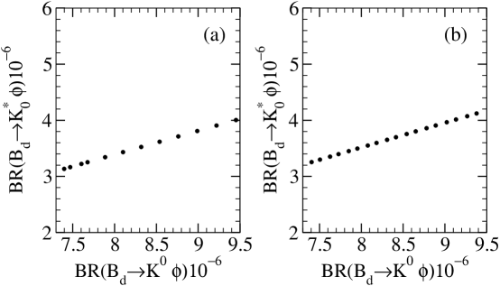
By using Eqs. (29) and (34), the correlation in BRs between $B_{d}\to K^{*0}_{0}(1430)\phi$ and $B_{d}\to K^{0}\phi$ decays is presented in Fig. 2, where (a) and (b) denote the cases of $N^{\rm eff}_{c}=2$ and $3$, respectively. From the figure, we see clearly that the results are similar in both cases and they are consistent with the observations by BABAR. In addition, due to the signs of the annihilation contributions being opposite in $K^{0}\phi$ and $K^{*0}_{0}(1430)\phi$ modes, from the figure we also see that the BRs of $B_{d}\to K^{0}\phi$ and $B_{d}\to K^{*0}_{0}(1430)\phi$ increase simultaneously.

Figure 2: Correlations between $BR(B_{d}\to K^{0}\phi)$ and $BR(B_{d}\to K^{*0}_{0}(1430)\phi)$ at $\mu=2.5$ GeV with (a) $N^{\rm eff}_{c}=2$ and (b) $N^{\rm eff}_{c}=3$.

Next, we consider the decays of $B_{d}\to(K^{*0},\,K^{*0}_{2}(1430))\phi$. Similar to $B_{d}\to K^{0}\phi$, to determine $\tilde{A}^{K^{*}\phi}$ and $\tilde{V}^{K^{*}\phi}_{1,2}$, we use the world average values with $2\sigma$ errors for BR and PFs and $1\sigma$ errors for relative angles as

$$7.7\leq BR(B_{d}\to K^{*0}\phi)10^{6}\leq 11.3\,,$$

$$0.45\leq R_{L}(B_{d}\to K^{*0}\phi)\leq 0.53\,,\ \ \ 0.21\leq R_{\perp}(B_{d}\to K^{*0}\phi)\leq 0.35\,,$$

$$2.25\leq\phi_{\parallel}({\rm rad})\leq 2.59\,,\ \ \ 2.35\leq\phi_{\perp}({\rm rad})\leq 2.69\,,$$ (40)

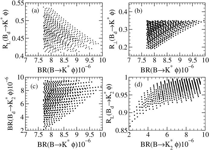
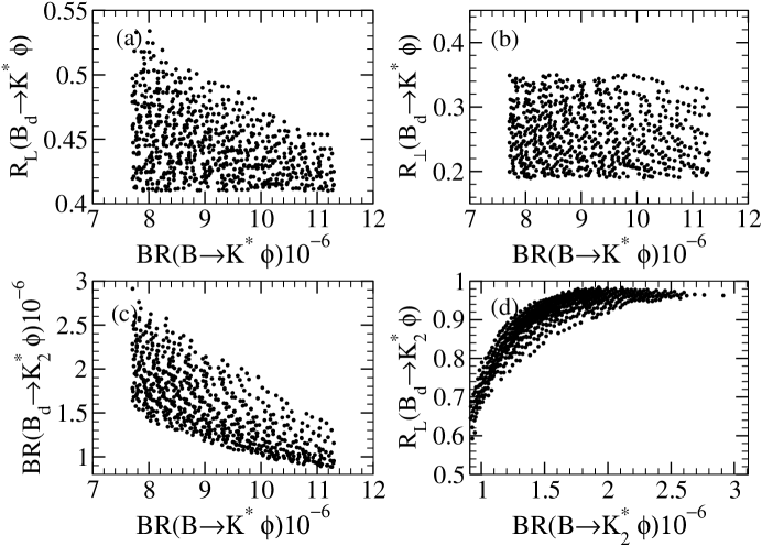
where the angles are defined by $\phi_{\parallel(\perp)}=Arg(A_{\parallel(\perp)}/A_{L})$. In terms of the constraints in Eq. (40) and Eqs. (II), (25), (30), (31) and Eq. (35), we present the results with the form factors in the LFQM (ISGW2) and $N^{\rm eff}_{c}=3$ in Fig. 3 (4). In both figures, the plots (a) [(b)] denote the correlations between $BR(B_{d}\to K^{*0}\phi)$ and $R_{L}(B_{d}\to K^{*0}\phi)[R_{\perp}(B_{d}\to K^{*0}\phi)]$. We note our results, which are consistent with data, indicate that the annihilated effects are important for the PFs. The plots (c)[(d)] display the correlations between $BR(B_{d}\to K^{*0}_{2}(1430)\phi)$ and $BR(B_{d}\to K^{*0}\phi)[R_{L}(B_{d}\to K^{*0}_{2}(1430)\phi)]$. From Figs. 3c and 4c, we see that $BR(B_{d}\to K^{*0}_{2}(1430)\phi)$ by the LFQM is much larger than that in the ISGW2. Moreover, the former is more favorable to the BABAR’s observation. From Figs. 3d and 4d, although $R_{L}$ in the ISGW2 could be lower, with the BR observed by BABAR, both QCD approaches predict a large longitudinal polarization in $B_{d}\to K^{*0}_{2}(1430)\phi$. According to our analysis, we conclude that $R_{L}(B\to K^{*}_{2}(1430)\phi)$ is $O(1)$ with or without including the annihilation contributions. Finally, we note that the results of $N^{\rm eff}_{c}=2$ are similar to those of $N^{\rm eff}_{c}=3$.

Figure 3: Correlations between (a)[(b), (c)] $BR(B_{d}\to K^{*0}\phi)$ and $R_{L}(B_{d}\to K^{*0}\phi)[R_{\perp}(B_{d}\to K^{*0}\phi),\,BR(B_{d}\to K^{*0}_{2}(1430)\phi)]$ and (d) $R_{L}$ and $BR(B_{d}\to K^{*0}_{2}(1430)\phi))$ in the LFQM.

Figure 4: Legend is the same as Fig. 3 but in the ISGW2.

IV Conclusions

We have studied the BRs for $B_{d}\to(K^{(*)0},\,K^{*0}_{n}(1430))\phi$ decays and the PFs for $B_{d}\to(K^{*0},\,K^{*0}_{2}(1430))\phi$ with and without the annihilation contributions. Since the QCD calculations on the time-like form factors are not as good as the transition form factors, we regard them as parameters fixed by the experimental measurements in $B_{d}\to K^{(*)0}\phi$. In terms of the ansatz by correlating the time-like form factors of $\langle K^{*}_{n}(1430)\phi|(V-A)_{\mu}|0\rangle$ to those of $\langle K^{(*)}\phi|(V-A)_{\mu}|0\rangle$, we find that $BR(B_{d}\to K^{*0}_{0}(1430)\phi)$ is $(3.86\pm 0.73)\times 10^{-6}$ and because of the annihilation contributions to $B\to K^{*}_{2}\phi$ and $B\to K^{*}\phi$ being opposite in sign, the longitudinal polarization of $B_{d}\to K^{*0}_{2}(1430)\phi$ is always $O(1)$ unlike those in $B\to K^{*}\phi$ decays. Due to the large differences in the transition form factors of $B\to K^{*}_{2}$ between the LFQM and ISGW2, we have shown that the former gives a broad allowed $BR(B_{d}\to K^{*0}_{2}(1430)\phi)$ and the latter limits it to be $(1.69\pm 0.81)\times 10^{-6}$. In terms of the recent BABAR’s observations on BRs and PFs of $B_{d}\to K^{*0}_{2}(1430)\phi$, the results based on the LFQM are more favorable.

Acknowledgments

This work is supported in part by the National Science Council of R.O.C. under Grant #s:NSC-95-2112-M-006-013-MY2 and NSC-95-2112-M-007-059-MY3.

References

(1)BELLE Collaboration, J. Zhang et al. , Phys. Rev. Lett. 91,
221801 (2003); K. Abe et al., arXiv:hep-ex/0507039.
(2) BELLE Collaboration, A. Somov et al., Phys. Rev. Lett. 96, 171801 (2006).
(3)BABAR Collaboration, B. Aubert et al., Phys. Rev. Lett.
91, 171802 (2003); A. Gritsan, arXiv:hep-ex/0409059.
(4)BABAR Collaboration, B. Aubert et al., Phys. Rev. D69, 031102 (2004);
Phys. Rev. Lett. 93, 231801 (2004); B. Aubert et al.,
Phys. Rev. D71, 031103 (2005).
(5) BELLE Collaboration, K. Abe et al., Phys. Lett. B538, 11 (2002);
arXiv:hep-ex/0408104.
(6) BABAR Collaboration, B. Aubert et al.,
Phys. Rev. Lett. 87, 241801 (2001).
(7)BELLE Collaboration, K. F. Chen, et al., Phys. Rev. Lett. 94, 221804 (2005).
(8)BABAR Collaboration, B. Aubert et al.,
arXive:hep-ex/0303020; B. Aubert et al., Phys. Rev. Lett. 93, 231804 (2004).
(9)A. Kagan, Phys. Lett. B601, 151 (2004).
(10)W.S. Hou and M. Nagashima,
hep-ph/0408007; P. Colangelo, F. De Fazio and T.N. Pham, Phys. Lett.
B597, 291 (2004); M. Ladisa et al., Phys. Rev. D70, 114025 (2004); H.Y. Cheng, C.K. Chua and A. Soni, Phys. Rev.
D71, 014030 (2005); H.N. Li, Phys. Lett. B622, 63
(2005).
(11)C.H. Chen, arXive:hep-ph/0601019.
(12)M. Beneke, J. Rohrer and D. Yang,
arXive:hep-ph/0612290.
(13) A. Kagan, hep-ph/0407076; E. Alvarez et al, Phys. Rev. D70,
115014 (2004); Y.D. Yang, R.M. Wang and G.R. Lu, Phys. Rev. D72, 015009 (2005); A.K. Giri and R. Mohanta, hep-ph/0412107; P.K.
Das and K.C. Yang, Phys. Rev. D71, 094002 (2005); C.S. Kim and
Y.D. Yang, arXiv:hep-ph/0412364, C.S. Hung et al., Phys. Rev.
D73, 034026 (2006); S. Nandi and A. Kundu, J. Phys. G32,
835 (2006) S. Baek et al., Phys. Rev. D72, 094008
(2005); A.R. Williamson and J. Zupan, Phys. Rev. D74, 014003
(2006); Erratum ibid D74, 03901 (2006); Qin Chang, X.Q.
Li and Y.D. Yang, arXive:hep-ph/0610280.
(14)C.H. Chen and C.Q. Geng, Phys. Rev. D71, 115004
(15)BABAR Collaboration, B. Aubert et al.,
arXive:hep-ex/0610073.
(16) G. Buchalla, A.J. Buras and M.E. Lautenbacher, Rev.
Mod. Phys. 68, 1125 (1996).
(17) N. Cabibbo, Phys. Rev. Lett. 10, 531 (1963); M. Kobayashi and T. Maskawa, Prog. Theor. Phys.
49, 652 (1973).
(18) J. D. Bjorken, Nucl. Phys. Proc. Suppl. 11, 325 (1989).
(19)P. Ball and R. Zwicky, Phys. Rev. D71, 014015
(2005); ibid, 71, 014029 (2005); Phys. Lett. B633,
289 (2006); JHEP 0602, 034 (2006); JHEP 0605, 004
(2006).
(20) A. Ali, G. Kramer and C.D. Lu,
Phys. Rev. D58, 094009 (1998).
(21) Y.H. Chen et al., Phys. Rev D60,
094014 (1999).
(22) M. Bauer, B. Stech and M. Wirbel, Z. Phys. C34,