Decays of $J/\psi$ and $\psi^{\prime}$ into vector and pseudoscalar meson and the pseudoscalar glueball-$q\bar{q}$ mixing

Abstract

We introduce a parametrization scheme for $J/\psi(\psi^{\prime})\to VP$ where the effects of SU(3) flavor symmetry breaking and doubly OZI-rule violation (DOZI) can be parametrized by certain parameters with explicit physical interpretations. This scheme can be used to clarify the glueball-$q\bar{q}$ mixing within the pseudoscalar mesons. We also include the contributions from the electromagnetic (EM) decays of $J/\psi$ and $\psi^{\prime}$ via $J/\psi(\psi^{\prime})\to\gamma^{*}\to VP$. Via study of the isospin violated channels, such as $J/\psi(\psi^{\prime})\to\rho\eta$, $\rho\eta^{\prime}$, $\omega\pi^{0}$ and $\phi\pi^{0}$, reasonable constraints on the EM decay contributions are obtained. With the up-to-date experimental data for $J/\psi(\psi^{\prime})\to VP$, $J/\psi(\psi^{\prime})\to\gamma P$ and $P\to\gamma\gamma$, etc, we arrive at a consistent description of the mentioned processes with a minimal set of parameters. As a consequence, we find that there exists an overall suppression of the $\psi^{\prime}\to 3g$ form factors, which sheds some light on the long-standing “$\rho\pi$ puzzle”. By determining the glueball components inside the pseudoscalar $\eta$ and $\eta^{\prime}$ in three different glueball-$q\bar{q}$ mixing schemes, we deduce that the lowest pseudoscalar glueball, if exists, has rather small $q\bar{q}$ component, and it makes the $\eta(1405)$ a preferable candidate for $0^{-+}$ glueball.

PACS numbers: 13.20.Gd, 12.40.Vv, 13.25.-k, 12.39.Mk

I Introduction

Charmonium decays into light hadrons provides unique places to probe light hadron structures. In particular, in the hadronic decays of charmonia such as $J/\psi$, $\eta_{c}$ and $\chi_{cJ}$ etc, the annihilation of the heavy $c\bar{c}$ pair into intermediate gluons, which must be then hadronized into hadrons, could favor the production of unconventional hadrons such as glueball and hybrids in the final-state. Such states, different from the conventional $q\bar{q}$ or $qqq$ structures in the non-relativistic constituent quark model, can serve as a direct test of QCD as a non-Abelian gauge theory.

In the past decades, the exclusive hadronic decays of $J/\psi(\psi^{\prime})\to VP$ have attracted a lot of attention in both experiment and theory. These processes, in which the helicity is non-conserved, must be suppressed according to the selection rule of pQCD hadronic helicity conservation due to the vector nature of gluons [1]. According to the “pQCD power” suppression of helicity conservation and breaking, one should have $BR(\psi^{\prime}\to\rho\pi)/BR(J/\psi\to\rho\pi)\simeq(M_{J/\psi}/M_{\psi^{\prime}})^{6}\sim 0.35$ [1]. However, the experimental data show that this ratio is badly violated in reality, $BR(\psi^{\prime}\to\rho\pi)/BR(J/\psi\to\rho\pi)\simeq(0.2\pm 0.1)\%$ [2], i.e. much greatly suppressed. It led to the so-called “$\rho\pi$ puzzle” in the study of $J/\psi$ and $\psi^{\prime}$ exclusive decays, and initiated a lot of interests to the relevant issues [3, 4, 5, 6, 7, 8, 9, 10, 11, 12, 13, 14, 15, 16, 17]. An alternative expression of the “$\rho\pi$ puzzle” is via the ratios between $J/\psi$ and $\psi^{\prime}$ annihilating into three gluons and a single photon:

$$R \equiv \frac{BR(\psi^{\prime}\to hadrons)}{BR(J/\psi\to hadrons)}$$ (1)

$$\simeq \frac{BR(\psi^{\prime}\to e^{+}e^{-})}{BR(J/\psi\to e^{+}e^{-})}\simeq 12\%,$$

which is empirically called “12% rule”. Since most of those exclusive decays for $J/\psi$ and $\psi^{\prime}$ seem to abide by this empirical rule reasonably well, it is puzzling that the ratios for $\rho\pi$ and $K^{*}\bar{K}+c.c.$ deviate dramatically from it. A recent article by Mo, Yuan and Wang provides a detailed review of the present available explanations (see Ref.  [18] and references therein).

A catch-up of this subject is an analysis by authors here for the electromagnetic decays of $J/\psi(\psi^{\prime})\to\gamma^{*}\to VP$ [19]. There, it is shown that although the EM contributions to $J/\psi\to VP$ are generally small relative to the strong decays as found by many other studies [20], they may turn to be more competitive in $\psi^{\prime}\to VP$ compared with $\psi^{\prime}\to 3g\to VP$ amplitudes, and produce crucial interferences [19]. For a better understanding of the “$\rho\pi$ puzzle”, a thorough study of $J/\psi(\psi^{\prime})\to VP$ including both strong and EM transitions and accommodating the up-to-date experimental information [21, 22, 23, 24] should be necessary.

The reaction channels $J/\psi(\psi^{\prime})\to VP$ also give access to another interesting issue in non-perturbative QCD. They may be used to probe the structure of the isoscalar $0^{-+}$, i.e. $\eta$ and $\eta^{\prime}$ in their recoiling isoscalar vector mesons $\omega$ or $\phi$. Since vector meson $\omega$ and $\phi$ are almost ideally mixed, i.e. $\omega=(u\bar{u}+d\bar{d})/\sqrt{2}$ and $\phi=s\bar{s}$, the decay of $J/\psi(\psi^{\prime})\to\omega\eta$, $\omega\eta^{\prime}$, $\phi\eta$, and $\phi\eta^{\prime}$ will provide information about $\eta$ and $\eta^{\prime}$, which can be produced via the so-called singly OZI disconnected (SOZI) processes for the same flavor components, and doubly OZI disconnected (DOZI) processes for different flavor components.

Nonetheless, it can also put experimental constraints on the octet-singlet mixing as a consequence of the $U(1)_{A}$ anomaly of QCD [25, 28, 29, 30, 31, 26, 27, 32, 33]. Recently, Leutwyler [32], and Feldmann and his collaborators [33] propose a $\eta$-$\eta^{\prime}$ mixing scheme in the quark flavor basis with an assumption that the decay constants follow the pattern of particle state mixing, and thus are controlled by specific Fock state wavefunctions at zero separation of the quarks, while the state mixing is referred to the mixing in the overall wavefunctions. In the quark flavor basis it is shown that higher Fock states (specifically, $|gg\rangle$) due to the anomaly give rise to a relation between the mixing angle and decay constants. This analysis brings the question of gluon components inside $\eta$ and $\eta^{\prime}$ to much closer attention from both experiment and theory [33, 34], and initiates a lot of interests in the pseudoscalar sector, in particular, in line with the search for pseudoscalar glueball candidates.

The lattice QCD (LQCD) calculations predict a mass for the lowest pseudoscalar glueball around 2.5 GeV [35], which is higher than a number of $0^{-+}$ resonances observed in the range of 1$\sim$ 2.3 GeV. However, since the present LQCD calculations are based on quenched approximation, the glueball spectrum is still an open question in theory. In contrast, QCD phenomenological studies [36, 37, 38, 39] favor a much lower $0^{-+}$ glueball mass, and make $\eta(1405)$ a good glueball candidate due to its strong couplings to $K\bar{K}\pi$ and $a_{0}(980)\pi$ and absence in $\gamma\gamma\to K\bar{K}\pi$ and $\eta\pi\pi$ [2]. Study of $J/\psi\to VP$ in flavor parametrization schemes was pursued in Ref. [20], where the $\eta$ and $\eta^{\prime}$ were treated as eigenstates of $q\bar{q}$. By assuming the $\eta(1405)$ to be a glueball essentially and introducing a DOZI suppression factor for $\phi G$ and $\omega G$ amplitudes relative to the SOZI processes, the authors seemed to have underestimated the branching ratios for $BR(J/\psi\to\phi\eta(1405))$ and $BR(J/\psi\to\omega\eta(1405))$. In Ref. [40] a mixing scheme for $\eta$, $\eta^{\prime}$ and $\eta(1405)$ in a basis of $(u\bar{u}+d\bar{d})/\sqrt{2}$, $s\bar{s}$ and $G$ (glueball) was proposed and studied in $J/\psi\to VP$. $\eta(1405)$ was found to be dominated by the glueball component, while the glueball component in $\eta^{\prime}$ was also sizeable. In both studies, the EM contributions were included as a free parameter in $J/\psi\to VP$. However, as we now know that the EM contributions in $\psi^{\prime}$ are important [19]. Thus, a coherent study of $J/\psi(\psi^{\prime})\to VP$ including the EM contributions would be ideal for probing the structure of the pseudoscalar mesons.

On the theoretical side there is only one possible term in the effective Lagrangian for $J/\psi(\psi^{\prime})\to VP$ and it will reduce the number of the parameters needed in phenomenological studies. On the experimental side many new data with high accuracy are available. Hence, in this work, we shall revisit $J/\psi(\psi^{\prime})\to VP$ trying to clarify the following points: (i) What is the role played by the EM decay transitions? By isolating and constraining the EM transitions in a VMD model, we propose a parametrization scheme for the strong transitions where the SU(3) flavor symmetry breaking and DOZI violation effects can be accommodated. A reliable calculation of the EM transitions in turn will put a reasonable constraint on the strong decay transitions in $J/\psi(\psi^{\prime})\to VP$, and thus mechanisms leading to the “$\rho\pi$ puzzle” can be highlighted. (ii) We shall probe the glueball components within $\eta$ and $\eta^{\prime}$ based on the available experimental data and different quarkonia-glueball mixing schemes, and predict the $0^{-+}$ glueball production rate in $J/\psi(\psi^{\prime})$ hadronic decays.

As follows, we first present the parametrization scheme for $J/\psi(\psi^{\prime})\to VP$ and introduce the glueball components into the pseudoscalars. We then briefly discuss the VMD model for $J/\psi(\psi^{\prime})\to\gamma^{*}\to VP$. In Section III, we present the model calculation results with detailed discussions. A summary will be given in Section IV.

II Model for $J/\psi(\psi^{\prime})\to VP$

In this Section, we first introduce a simple rule to parametrize out the strong decays of $J/\psi(\psi^{\prime})\to VP$. We then introduce a VMD model for the $J/\psi(\psi^{\prime})$ EM decays into $VP$. A recent study of $J/\psi(\psi^{\prime})\to\gamma^{*}\to VP$ shows that the EM decay contributions become important in $\psi^{\prime}$ decays due to its large partial decay width to $e^{+}e^{-}$ though their importance is not so significant in $J/\psi\to VP$ [19]. In the isoscalar pseudoscalar sector, we introduce three different glueball-$q\bar{q}$ mixing schemes for $\eta$, $\eta^{\prime}$ and a glueball candidate $\eta^{\prime\prime}$. Its production in $J/\psi(\psi^{\prime})$ hadronic decays can then be factorized out and estimated.

II.1 Decay of $J/\psi(\psi^{\prime})\to VP$ via strong interaction

The strong decay of $J/\psi(\psi^{\prime})\to VP$ via $3g$ can be factorized out in a way similar to Ref. [41].

First, we define the strength of the non-strange singly OZI disconnected (SOZI) process as

$$g_{J/\psi(\psi^{\prime})}\equiv\langle(q\bar{q})_{V}(q\bar{q})_{P}|V_{0}|J/\psi(\psi^{\prime})\rangle,$$ (2)

where $V_{0}$ denotes the $3g$ decay potential of the charmonia into two non-strange $q\bar{q}$ pairs of vector and pseudoscalar via SOZI processes. But it should be noted that the subscription $V$ and $P$ do not mean that the quark-antiquark pairs are flavor eigenstates of vector and pseudoscalar mesons. The amplitude $g_{J/\psi(\psi^{\prime})}$ is proportional to the charmonium wavefunctions at origin. Thus, it may have different values for $J/\psi$ and $\psi^{\prime}$.

In order to include the SU(3) flavor symmetry breaking effects in the transition, we introduce

$$R\equiv\langle(q\bar{s})_{V}(s\bar{q})_{P}|V_{0}|J/\psi(\psi^{\prime})\rangle/g_{J/\psi(\psi^{\prime})}=\langle(s\bar{q})_{V}(q\bar{s})_{P}|V_{0}|J/\psi(\psi^{\prime})\rangle/g_{J/\psi(\psi^{\prime})},$$ (3)

which implies the occurrence of the SU(3) flavour symmetry breaking at each vertex where a pair of $s\bar{s}$ is produced, and $R=1$ is in the SU(3) flavour symmetry limit. For the production of two $s\bar{s}$ pairs via the SOZI potential, the recognition of the SU(3) flavor symmetry breaking in the transition is accordingly

$$R^{2}\simeq\langle(s\bar{s})_{V}(s\bar{s})_{P}|V_{0}|J/\psi(\psi^{\prime})\rangle/g_{J/\psi(\psi^{\prime})}\ .$$ (4)

Similar to Ref. [41], the DOZI process is distinguished from the SOZI ones by the gluon counting rule. A parameter $r$ is introduced to describe the relative strength between the DOZI and SOZI transition amplitudes:

$$r\equiv\langle(s\bar{s})_{V}(q\bar{q})_{P}|V_{1}|J/\psi(\psi^{\prime})\rangle/g_{J/\psi(\psi^{\prime})}=\langle(q\bar{q})_{V}(s\bar{s})_{P}|V_{1}|J/\psi(\psi^{\prime})\rangle/g_{J/\psi(\psi^{\prime})},$$ (5)

where $V_{1}$ denotes the charmonium decay potential via the DOZI processes; In the circumstance that the OZI rule is respected, one expects $|r|\sim 0$.

Through the above definitions, we express the amplitudes for $J/\psi(\psi^{\prime})\to V(q\bar{q})_{P}$ as

$$M_{K^{*+}K^{-}} = \langle K^{*+}K^{-}|V_{0}|J/\psi(\psi^{\prime})\rangle=g_{J/\psi(\psi^{\prime})}R\ ,$$ (6)

$$M_{\rho^{+}\pi^{-}} = \langle\rho^{+}\pi^{-}|V_{0}|J/\psi(\psi^{\prime})\rangle=g_{J/\psi(\psi^{\prime})}\ ,$$ (7)

$$M_{\rho^{0}\pi^{0}} = \langle\rho^{0}\pi^{0}|V_{0}|J/\psi(\psi^{\prime})\rangle=g_{J/\psi(\psi^{\prime})}\ ,$$ (8)

$$M_{\phi(s\bar{s})} = \langle\phi(s\bar{s})_{P}|V_{0}+V_{1}|J/\psi(\psi^{\prime})\rangle=R^{2}g_{J/\psi(\psi^{\prime})}(1+r),$$ (9)

$$M_{\phi(n\bar{n})} = \langle\phi(n\bar{n})_{P}|V_{1}|J/\psi(\psi^{\prime})\rangle=\sqrt{2}r\langle\phi(s\bar{s})_{P}|V_{0}|J/\psi(\psi^{\prime})\rangle=\sqrt{2}rRg_{J/\psi(\psi^{\prime})},$$ (10)

$$M_{\omega(s\bar{s})} = \langle\omega(s\bar{s})_{P}|V_{1}|J/\psi(\psi^{\prime})\rangle=\sqrt{2}Rrg_{J/\psi(\psi^{\prime})},$$ (11)

$$M_{\omega(n\bar{n})} = \langle\omega(n\bar{n})_{P}|V_{0}+V_{1}|J/\psi(\psi^{\prime})\rangle=g_{J/\psi(\psi^{\prime})}(1+2r),$$ (12)

where the channels $K\bar{K^{*}}$ and $\rho^{-}\pi^{+}$ have the same expressions as their conjugate channels; $n\bar{n}\equiv(u\bar{u}+d\bar{d})/\sqrt{2}$ is the non-strange isospin singlet. We have assumed that $\phi$ and $\omega$ are ideally mixed and they are pure $s\bar{s}$ and $n\bar{n}$, respectively.

The recoiled pseudoscalars by $\phi$ and $\omega$ can be either $\eta$ or $\eta^{\prime}$ for which we consider that a small glueball component will mix with the dominant $q\bar{q}$ in the quark flavour basis. The detailed discussion about the $q\bar{q}$ and glueball mixings in $\eta$ and $\eta^{\prime}$ will be given in the next section. Here, we relate the production of glueball $G$ in $J/\psi(\psi^{\prime})\to\omega G$ and $\phi G$ with the basic amplitude $g_{J/\psi(\psi^{\prime})}$ by assuming the validity of gluon counting rule in the transitions [41, 42], i.e.

$$\langle(q\bar{q})_{V}G|V_{3}|J/\psi(\psi^{\prime})\rangle\equiv g_{J/\psi(\psi^{\prime})}\ ,$$ (13)

where $V_{3}$ denotes the glueball $G$ production potential recoiling a flavour singlet $q\bar{q}$. This can be regarded as reasonable since generally the glueball does not pay a price for its couplings to gluons. Consequently, we have

$$M_{\phi G} = \langle\phi G|V_{3}|J/\psi(\psi^{\prime})\rangle=g_{J/\psi(\psi^{\prime})}R$$

$$M_{\omega G} = \langle\omega G|V_{3}|J/\psi(\psi^{\prime})\rangle=\sqrt{2}g_{J/\psi(\psi^{\prime})}\ ,$$ (14)

with the SU(3) flavor symmetry breaking considered for the $\phi$ production.

The above parametrization highlights several interesting features in those decay channels. It shows that the decay of $J/\psi(\psi^{\prime})\to\rho\pi$ is free of interferences from the DOZI processes and possible SU(3) flavor symmetry breaking. Ideally, such a process will be useful for us to determine $g_{J/\psi(\psi^{\prime})}$. The decay of $J/\psi(\psi^{\prime})\to K^{*}\bar{K}+c.c.$ is also free of DOZI interferences, but correlates with the SU(3) breaking. These two sets of decay channels will, in principle, allow us to determine the basic decay amplitude $g_{J/\psi(\psi^{\prime})}$ and the SU(3) flavor breaking effects, which can then be tested in other channels. For $\phi\eta$, $\phi\eta^{\prime}$, $\omega\eta$ and $\omega\eta^{\prime}$, the transition amplitudes will also depend on the $\eta$-$\eta^{\prime}$ mixing angles and we will present detailed discussions in later part.

In the calculation of the partial decay width, we must apply the commonly used form factor

$${\cal{F}}^{2}({\bf P})\equiv|{\bf P}|^{2l}\exp({-{\bf P}^{2}/{8\beta^{2}}}),$$ (15)

where ${\bf P}$ and the $l$ are the three momentum and the relative orbit angular momentum of the final-state mesons, respectively, in the $J/\psi(\psi^{\prime})$ rest frame. We adopt $\beta=0.5\mbox{GeV}$, which is the same as Refs. [43, 44, 42]. At leading order the decays of $J/\psi(\psi^{\prime})\to VP$ are via $P$-wave, i.e. $l=1$. This form factor accounts for the size effects from the spatial wavefunctions of the initial and final-state mesons.

II.2 Decay of $J/\psi(\psi^{\prime})\to VP$ via EM interaction

Detailed study of $J/\psi(\psi^{\prime})\to\gamma^{*}\to VP$ in a VMD model is presented in Ref. [19]. In this process, three independent transitions contribute to the total amplitude as shown by Fig. 2. The advantage of treating this process in the VMD model is to benefit from the available experimental information for all those coupling vertices. As a result the only parameter present in the EM transition amplitude is the form factor for the virtual photon couplings to the initial ($J/\psi$ and $\psi^{\prime}$) and final state vector mesons ($\omega$, $\phi$, $\rho$ and $K^{*}$). As shown in Ref. [19], the isospin violated channels, $\rho\eta$, $\rho\eta^{\prime}$, $\omega\pi$ and $\phi\pi$, provides a good constraint on the $\gamma^{*}VP$ form factors without interferences from the strong decays. Therefore, a reliable estimate of the EM transitions can be reached.

Following the analysis of Ref. [19], the invariant transition amplitude for $J/\psi\to\gamma^{*}\to VP$ at tree level can be expressed as:

$${\cal M}_{EM} \equiv {\cal M}_{A}+{\cal M}_{B}+{\cal M}_{C}$$ (16)

$$= \left(\frac{e}{f_{V2}}\frac{g_{V1\gamma P}}{M_{V1}}{\cal F}_{a}+\frac{e}{f_{V1}}\frac{g_{V2\gamma P}}{M_{V2}}{\cal F}_{b}+\frac{e^{2}}{f_{V1}f_{V2}}\frac{g_{P\gamma\gamma}}{M_{P}}{\cal F}_{c}\right)\epsilon_{\mu\nu\alpha\beta}\partial^{\mu}V_{1}^{\nu}\partial^{\alpha}V_{2}^{\beta}P,$$

where $e/f_{V}$ denotes the $\gamma^{*}V$ couplings, and $g_{V\gamma P}$ is the coupling determined in the radiative decay of $V\to\gamma V$; ${\cal F}_{a}$, ${\cal F}_{b}$ and ${\cal F}_{c}$ denote the form factors corresponding to the transitions of Fig. 2. For Fig. 2(a) and (b) a typical monopole (MP) form factor is adopted:

$${\cal F}(q^{2})=\frac{1}{1-q^{2}/\Lambda^{2}}$$ (17)

with $\Lambda=0.542\pm 0.008$ GeV and $\Lambda=0.577\pm 0.011$ GeV determined with a constructive (MP-C) or destructive phase (MP-D) between (a) and (b), respectively. We think that the non-perturbative QCD effects might have played a role in the transitions at $J/\psi$ energy. For instance, in Fig. 2(a) and (b) a pair of quarks may be created from vacuum as described by ${}^{3}P_{0}$ model, the pQCD hadronic helicity-conservation due to the vector nature of gluon is violated quite strongly. A monopole-like (MP) form factor should be appropriate for coping with the suppression effects, and it is consistent with the VMD framework. In principle such a form factor can be tested experimentally via measuring the couplings of the processes $J/\psi(\psi^{\prime})\to Pe^{+}e^{-}$ and $e^{+}e^{-}\to Pe^{+}e^{-}$, respectively, when the integrated luminosity at $J/\psi$ and the suitable energies for $e^{+}e^{-}$ colliders is accumulated enough.

Due to an error of missing a factor of $\sqrt{2}$ in Tab. I of Ref. [19], we give here in Table 1 the coupling $e/f_{V}$ again. Also, we clarify that although the overall factor of $\sqrt{2}$ will change the fitted cut-off energy $\Lambda$ and the fitted branching ratios slightly in Ref. [19], the pattern obtained there retains and the major conclusion is intact.

The form factor for (c) has a form of:

$${\cal F}_{c}(q_{1}^{2},q_{2}^{2})=\frac{1}{(1-q_{1}^{2}/\Lambda^{2})(1-q_{2}^{2}/\Lambda^{2})}\ ,$$ (18)

where $q_{1}^{2}=M_{V1}^{2}$ and $q_{2}^{2}=M_{V2}^{2}$ are the squared four-momenta carried by the time-like photons. We assume that the $\Lambda$ is the same as in Eq. (17), thus, ${\cal F}_{c}={\cal F}_{a}{\cal F}_{b}$.

A parameter $\delta$ is introduced to take into account the relative phase between the EM and strong transitions:

$${\cal M}={\cal M}_{3g}+e^{i\delta}{\cal M}_{EM}\ .$$ (19)

It will then be determined by the experimental data in the numerical fitting. In the limit of $\delta=0$, the relative phase reduces to the same ones given in Ref. [20].

II.3 Mixing of the $\eta-\eta^{\prime}$ and implication of a $0^{-+}$ glueball

The $\eta-\eta^{\prime}$ mixing is a long-standing question in the literature. Here we would like to study the “mixing” problem by including empirically a possible glueball component in the $\eta$ and $\eta^{\prime}$ wavefunctions. We extend the mixing of the the $\eta$ and $\eta^{\prime}$ as a consequence of the flavor singlet $n\bar{n}$, $s\bar{s}$ and glueball mixing. The corresponding glueball candidate is denoted as $\eta^{\prime\prime}$. In the quark flavor basis, treating $\eta$, $\eta^{\prime}$ and $\eta^{\prime\prime}$ as the eigenstates of the mass matrix $M$ with the eigenvalues of their masses $M_{\eta}$, $M_{\eta^{\prime}}$ and $M_{\eta^{\prime\prime}}$, we have

$$UMU^{-1}=\left(\matrix{M_{\eta}&0&0\cr 0&M_{\eta^{\prime}}&0\cr 0&0&M_{\eta^{\prime\prime}}}\right),$$ (20)

where $U$ is the state mixing matrix:

$$\left(\matrix{\eta\cr\eta^{\prime}\cr\eta^{\prime\prime}}\right)=U\left(\matrix{n\bar{n}\cr s{\bar{s}}\cr G}\right)=\left(\matrix{x_{1}&y_{1}&z_{1}\cr x_{2}&y_{2}&z_{2}\cr x_{3}&y_{3}&z_{3}}\right)\left(\matrix{n\bar{n}\cr s{\bar{s}}\cr G}\right).$$ (21)

Three mixing schemes are applied to determine the mixing matrix elememts.

I) CKM approach

By assuming that the $n\bar{n}$, $s\bar{s}$ and glueball $G$ make a complete set of eigenstates, and physical states are their linear combinations, we can express the mixing in the same way as the CKM matrix with the phase $\delta=0$ (no $CP$ violation is involved):

$$U=\left(\matrix{c_{12}c_{13}&s_{12}c_{13}&s_{13}\cr-s_{13}c_{23}-c_{12}s_{23}s_{13}&c_{12}c_{23}-s_{12}s_{23}s_{13}&s_{23}c_{13}\cr s_{12}s_{23}-c_{12}c_{23}s_{13}&-c_{12}s_{23}-s_{12}c_{23}s_{13}&c_{23}c_{13}}\right)\ ,$$ (22)

where $c_{ij}\equiv\cos\theta_{ij}$ and $s_{ij}\equiv\sin\theta_{ij}$ with $\theta_{ij}$ the mixing angles to be determined by the experimental data. The feature of this approach is that the completeness guarantees the unitary and orthogonal relations of the matrix. However, it also implies that mixings beyond $q\bar{q}$ and glueball are not allowed. This may be a strong assumption since resonances and exotic states such as tetraquarks with the same quantum number could also mix with the $q\bar{q}$ and glueball. Because of this, the CKM approach will test the extreme condition that only ground state $q\bar{q}$ and $G$ mix with each other.

II) $q\bar{q}$-$G$ mixing due to higher Fock state $|gg\rangle$

This scenario is initiated by the QCD $U(1)_{A}$ anomaly. In a series of studies by Feldmann et al. [33, 34], it is pointed out that an appropriate treatment of the mixing requires to distinguish matrix elements of $\eta$ and $\eta^{\prime}$ with local currents and overall state mixings. Nonetheless, the divergences of axial-vector currents including the axial anomaly connect the short-distance properties, i.e. decay constants, with the long-distance phenomena such as the mass-mixing, and highlight the twist-4 $|gg\rangle$ component in the Fock state decomposition. In the quark flavor basis, higher Fock state due to anomaly can give rise to a non-vanishing $q\bar{q}\to|gg\rangle$ transition. Similar to the prescription of Ref. [33, 34], we introduce the glueball components in $\eta$ and $\eta^{\prime}$ via the higher Fock state decompositions in $\eta_{n}$ and $\eta_{s}$:

$$|\eta_{n}\rangle = \Psi_{q}|n\bar{n}\rangle+\Psi_{q}^{g}|gg\rangle+\cdots,$$

$$|\eta_{s}\rangle = \Psi_{s}|s\bar{s}\rangle+\Psi_{s}^{g}|gg\rangle+\cdots,$$ (23)

where $\Psi_{q}$ and $\Psi_{s}$ are amplitudes of the corresponding $q\bar{q}$ while $\Psi_{q}^{g}$ and $\Psi_{s}^{g}$ are those of the $|gg\rangle$ components; The dots denote higher Fock states with additional gluon and/or $q\bar{q}$ which is beyond the applicability of this approach. The presence of the gluonic Fock states in association with isoscalar $n\bar{n}$ and $s\bar{s}$ breaks the orthogonality between $n\bar{n}$ and $s\bar{s}$, and we parametrize such an effect in $\eta$ and $\eta^{\prime}$ wavefunctions:

$$|\eta\rangle = {1\over\sqrt{N_{1}}}[a(\cos{\phi}|n\bar{n}\rangle-\sin{\phi}|s\bar{s}\rangle)+b(\cos{\phi}-\sin{\phi})|gg\rangle],$$

$$|\eta^{\prime}\rangle = {1\over\sqrt{N_{2}}}[a(\sin{\phi}|n\bar{n}\rangle+\cos{\phi}|s\bar{s}\rangle)+b(\sin{\phi}+\cos{\phi})|gg\rangle],$$ (24)

where the normalization factors are $N_{1}=a^{2}+b^{2}(1-\sin{2\phi})$ and $N_{2}=a^{2}+b^{2}(1+\sin{2\phi})$, and parameters $a$ and $b$ are to be determined by experiment. In this treatment, $a$ and $b$ now correlate with the mixing angle $\phi\equiv\theta+\arctan\sqrt{2}$, with $\theta$ as the octet-singlet mixing angle defined in the SU(3) symmetry limit ($b\to 0$). For the commonly accepted range $\theta\simeq-24.6^{\circ}$ or $-11.5^{\circ}$ from the linear or quadratic mass formulae, respectively [2], the glueball component in $\eta$ has a strength of $b(\cos\phi-\sin\phi)/\sqrt{N_{1}}$, which is relatively suppressed in comparison with that in $\eta^{\prime}$, i.e. $b(\sin\phi+\cos\phi)/\sqrt{N_{2}}$, for $0^{\circ}<\phi<90^{\circ}$. This naturally gives rise to the scenario addressed in Ref. [33, 34].

Based on the unitary and orthogonal relation for three mixed states, we can derive:

$$\left\{\begin{array}[]{ccc}x_{3}^{2}&=&1-(x_{1}^{2}+x_{2}^{2}),\\ y_{3}^{2}&=&1-(y_{1}^{2}+y_{2}^{2}),\\ z_{3}^{2}&=&1-(z_{1}^{2}+z_{2}^{2}).\end{array}\right.$$ (25)

which will provide information about the $q\bar{q}$ and glueball components in $\eta^{\prime}$ though it is not necessary for the unitary and orthogonal relation being satisfied. If other higher Fock states which are negligible in $\eta$ and $\eta^{\prime}$ are present in $\eta^{\prime\prime}$ with sizable amplitude, further constraints on the mixing wavefunction for $\eta^{\prime\prime}$ will be needed.

III) Mixing in an old perturbation theory

Considering the mixing between quarkonia and glueball at leading order of a perturbation potential, i.e. the transition strength between two states are much smaller than the mass difference of these two states, we can then express the physical states as [43]

$$|\eta\rangle = \frac{1}{C_{1}}\left[|n\bar{n}\rangle+\frac{\sqrt{2}f_{b}}{M_{n\bar{n}}-M_{s\bar{s}}}|s\bar{s}\rangle+\frac{\sqrt{2}f_{a}}{M_{n\bar{n}}-M_{G}}|G\rangle\right]$$

$$|\eta^{\prime}\rangle = \frac{1}{C_{2}}\left[\frac{\sqrt{2}f_{b}}{M_{s\bar{s}}-M_{n\bar{n}}}|n\bar{n}\rangle+|s\bar{s}\rangle+\frac{\sqrt{2}f_{a}}{M_{s\bar{s}}-M_{G}}|G\rangle\right]$$

$$|\eta^{\prime\prime}\rangle = \frac{1}{C_{3}}\left[\frac{\sqrt{2}f_{a}}{M_{G}-M_{n\bar{n}}}|n\bar{n}\rangle+\frac{\sqrt{2}f_{a}}{M_{G}-M_{s\bar{s}}}|s\bar{s}\rangle+|G\rangle\right],$$ (26)

where $f_{a}\equiv\langle s\bar{s}|V_{g}|G\rangle=\langle n\bar{n}|V_{g}|G\rangle/\sqrt{2}$ is the mixing strength for glueball-$q\bar{q}$ transitions, while $f_{b}\equiv\langle q\bar{q}|V_{q}|s\bar{s}\rangle$ is the $s\bar{s}$ and non-strange $q\bar{q}$ mixing strength via transition potential $V_{q}$. $C_{1,2,3}$ are the normalization factors. $M_{n\bar{n}}$, $M_{s\bar{s}}$ and $M_{G}$ are masses for the pure $0^{-+}$ quarkonia and glueball states, respectively. They will be determined with parameters $f_{a}$ and $f_{b}$ by fitting the experimental data to satisfy the the physical masses for $\eta$, $\eta^{\prime}$ and $\eta^{\prime\prime}$, and unitary and orthogonal relations.

The above three parametrization schemes address different aspects correlated with the glueball-$q\bar{q}$ mixing. The CKM approach automatically satisfies the unitary and orthogonal relations, and allows the mixing exclusively among those three states. In reality, this may not be the case, and other configurations with the same quantum number may also be present in the wavefunctions. The second scheme introducing quarkonia-glueball mixing within $\eta$ and $\eta^{\prime}$ via higher Fock state. In principle, there is no constraint on the $\eta^{\prime\prime}$ configuration. Thus, unitary and orthogonal relations do not necessarily apply to those three states. The third scheme applies the old perturbation theory and considers the non-vanishing transitions between those pure states. As a result, a physical state will be a mixture of quarkonia-glueball configurations. The unitary and orthogonal relations will be a constraint in the determination of the parameters. Comparing these three different parametrization schemes, we expect that the quarkonia-glueball mixing mechanism and implication of the pseudoscalar glueball candidate can be highlighted.

In Table 2, the transition amplitudes for the strong decays of $J/\psi(\psi^{\prime})\to VP$ are given.

III Numerical results

With the above preparations, we do the numerical calculations and present the results in this section.

III.1 Parameters and fitting scheme

The parameters introduced in these three different approaches can be classified into two classes. One consists of parameters which are commonly defined in all three schemes, such as $g_{J/\psi(\psi^{\prime})}$, $r$ and $R$, and $\delta$. Parameter $g_{J/\psi(\psi^{\prime})}$ is the basic transition strength for $J/\psi(\psi^{\prime})\to VP$, and proportional to the wavefunctions at origin for $J/\psi(\psi^{\prime})$. Obviously, it has different values for $J/\psi$ and $\psi^{\prime}$ decays, respectively. Parameter $R$ and $r$ are the relative strengths of the SU(3) flavor symmetry breaking and DOZI violation processes to $g_{J/\psi(\psi^{\prime})}$. They can also have different values in $J/\psi$ and $\psi^{\prime}$ decays. Parameter $\delta$ indicates the relative phases between the strong and EM transition amplitudes.

The other class consists of parameters for quarkonia-glueball mixings, for instance, the mixing angles in the CKM approach, and masses $M_{n\bar{n}}$, $M_{s\bar{s}}$, and $M_{G}$ for the $0^{-+}$ quarkonia and glueball, respectively. These parameters depend on the mixing schemes, and as mentioned earlier they give rise to different scenarios concerning the $\eta$ and $\eta^{\prime}$ mixings. We shall discuss their properties in association with the numerical results in the next section.

It should be noted that in the VMD model for the EM decay transitions [19] all couplings are determined independently by accommodating the experimental information for $V_{1}(V_{2})\to e^{+}e^{-}$, $P\to\gamma\gamma$, and $V_{1}(V_{2})\to\gamma P$ or $P\to\gamma V_{2}$, where $V_{1}=J/\psi$ or $\psi^{\prime}$, $V_{2}=\omega$, $\phi$, $\rho$, or $K^{*}$, and $P=\pi$, $\eta$, $\eta^{\prime}$ or $K$. This is essential for accounting for the EM contributions properly. Meanwhile, the radiative decays, such as $V\to\gamma\eta$ and $\gamma\eta^{\prime}$, $\eta\to\gamma\gamma$ and $\eta^{\prime}\to\gamma\gamma$, can probe the $q\bar{q}$ structure of the vector and pseudoscalar mesons. Their constraints on the $\eta$ and $\eta^{\prime}$ mixing have been embedded in constraining the EM transitions. As shown in Ref. [19], all the experimental data for $V_{1}(V_{2})\to e^{+}e^{-}$, $P\to\gamma\gamma$, and $V_{1}(V_{2})\to\gamma P$ or $P\to\gamma V_{2}$ have been included.

Given a reliable description of the EM transitions, we can then proceed to determine the strong transition parameters and configuration mixings within the pseudoscalars by fitting the data for $J/\psi(\psi^{\prime})\to VP$. The numerical study step is taken as follows: i) Fit the data for $J/\psi(\psi^{\prime})\to VP$ with only the strong decay transitions; ii) Fit the data for $J/\psi(\psi^{\prime})\to VP$ including the EM decay contributions. Comparing those two situations, information about the role played by the EM transitions, and their correlations with the strong decay amplitudes can thus be extracted. The $\eta$ and $\eta^{\prime}$ configurations can also be constrained. We emphasize that a reasonable estimate of the EM contributions is a prerequisite for a better understanding of the underlying mechanisms in $J/\psi(\psi^{\prime})\to VP$.

III.2 Numerical results and analysis

For each of these three parametrization schemes, three cases are examined: i) with exclusive contributions from $J/\psi(\psi^{\prime})$ strong decays; ii) with a MP-D form factor for the EM transitions; and iii) with a MP-C form factor for the EM transitions. The parameters are listed in Table 3-5, and the fitting results are listed in Tables 7 and 8 for $J/\psi$ and $\psi^{\prime}$, respectively.

In general, without the EM contributions the fitting results have a relatively larger $\chi^{2}$ value. With the EM contributions, the results are much improved for both MP-D and MP-C model. To be more specific, we first make an analysis of the commonly defined parameters, i.e. $g_{J/\psi(\psi^{\prime})}$, $r$, $R$ and $\delta$, and then discuss the quarkonia-glueball mixing parameters for each scheme.

For those commonly defined parameters their fitted values turn to be consistent with each other in those three schemes. It is interesting to compare the fitted values for the basic transition amplitude $g_{J/\psi(\psi^{\prime})}$ for $J/\psi$ and $\psi^{\prime}$. It shows that the inclusion of the EM contributions will bring significant changes to this quantity in $\psi^{\prime}$ decays, while it keeps rather stable in $J/\psi$ decays. This agrees with the observation that the EM contributions in $J/\psi$ hadronic decays are less significant relative to the strong ones [20, 40]. The absolute value of $g_{J/\psi(\psi^{\prime})}$ for $\psi^{\prime}$ is naturally smaller than that for $J/\psi$. Since $g_{J/\psi(\psi^{\prime})}$ is proportional to the wavefunctions at origins [19], the small fraction, $[g_{\psi^{\prime}}/g_{J/\psi}]^{2}\simeq 0.018$, implies an overall suppression of the $\psi^{\prime}\to 3g$ form factors in $\psi^{\prime}\to VP$, which is smaller than the pQCD expectation, $\sim 12\%$. It is worth noting that this suppression occurs not only to $\rho\pi$, but also to all the other $VP$ channels. We shall come back to this point in the later part.

Parameter $r$, denoting the OZI-rule violation effects, turns to be sizeable in $J/\psi$ decays but smaller in $\psi^{\prime}$ decays though relatively large uncertainties are accompanying. This is consistent with our expectation that the DOZI processes in $\psi^{\prime}$ decays will be relatively suppressed in comparison with those in $J/\psi$ decays. However, it is noticed that $r$ has quite large uncertainties in $\psi^{\prime}$ decays though the central values are small. This reflects that data for $\psi^{\prime}$ decays still possess relatively large errors, and increased statistics may better constrain this parameter.

The SU(3) breaking parameter exhibits an overall consistency in the fittings. Relatively large SU(3) flavor symmetry breaking turns to occur in the $J/\psi$ decays compared with that in $\psi^{\prime}$. In the case without EM contributions, the SU(3) breaking in $\psi^{\prime}$ decays also turns to be large. This may reflect the necessity of including the EM contributions. It shows that the SU(3) symmetry breaking in $J/\psi$ can be as large as about $34\%$, while it is about 5-20% in $\psi^{\prime}$ decays.

The phase angle $\delta$ is fitted for $J/\psi$ and $\psi^{\prime}$, respectively, when the EM contributions are included. It shows that $J/\psi$ favors a complex amplitude introduced by the EM transitions. In contrast, the strong and EM amplitudes in $\psi^{\prime}$ decays is approximately out of phase. This means that the strong and EM transitions will have destructive cancellations in $\rho\pi$, $K^{*+}K^{-}+c.c.$, but constructively interfere with each other in $K^{*0}\bar{K^{0}}+c.c.$ As qualitatively discussed in Ref. [19], this phase can lead to further suppression to $\psi^{\prime}\to\rho\pi$, and also explain the difference between $K^{*+}K^{-}+c.c.$ and $K^{*0}\bar{K^{0}}+c.c.$ The relative phases are in agreement with the results of Ref. [14], but different from those in Ref. [16].

III.2.1 CKM approach

In this mixing scheme it shows that mixing angles $\theta_{12}$ and $\theta_{23}$ are well constrained by the experimental data while large uncertainties occur to $\theta_{13}$ when the EM transitions are included. The corresponding matrix element $\sin\theta_{12}$ favors a small value which implies small glueball component inside $\eta$ meson. The mixed wavefunctions obtained with different EM interferences are:

$$\mbox{without EM : \ \ \ }\left\{\begin{array}[]{ccl}|\eta\rangle&=&0.915|n\bar{n}\rangle-0.404|s\bar{s}\rangle+0.003|G\rangle\\ |\eta^{\prime}\rangle&=&-0.398|n\bar{n}\rangle-0.903|s\bar{s}\rangle-0.163|G\rangle\\ |\eta^{\prime\prime}\rangle&=&0.068|n\bar{n}\rangle+0.148|s\bar{s}\rangle-0.987|G\rangle\end{array}\right.\ ;$$ (27)

$$\mbox{MP-D Model: \ \ \ }\left\{\begin{array}[]{ccl}|\eta\rangle&=&0.904|n\bar{n}\rangle-0.427|s\bar{s}\rangle+1.44\times 10^{-5}|G\rangle\\ |\eta^{\prime}\rangle&=&-0.421|n\bar{n}\rangle-0.892|s\bar{s}\rangle-0.166|G\rangle\\ |\eta^{\prime\prime}\rangle&=&0.071|n\bar{n}\rangle+0.150|s\bar{s}\rangle-0.986|G\rangle\end{array}\right.\ ;$$ (28)

and

$$\mbox{MP-C Model: \ \ \ }\left\{\begin{array}[]{ccl}|\eta\rangle&=&0.901|n\bar{n}\rangle-0.433|s\bar{s}\rangle+5.0\times 10^{-7}|G\rangle\\ |\eta^{\prime}\rangle&=&-0.427|n\bar{n}\rangle-0.888|s\bar{s}\rangle-0.168|G\rangle\\ |\eta^{\prime\prime}\rangle&=&0.073|n\bar{n}\rangle+0.151|s\bar{s}\rangle-0.986|G\rangle\end{array}\right.\ .$$ (29)

It shows that though $\theta_{13}$ has large uncertainties, its central values indicate a small glueball component in $\eta$. In particular, we find $\sin\theta_{13}\simeq 0$ in the MP-D model, while $\sin\theta_{13}=0.003$ or $5.0\times 10^{-7}$ from the calculations without EM contributions or in the MP-C model, respectively. In contrast, the amplitude of the glueball component in the $\eta^{\prime}$ wavefunction is much larger. In all three models (and also in all three mixing schemes), a stable glueball mixing magnitude of $\sim 17\%$ is favored.

The automatically satisfied unitary and orthogonal conditions lead to the prediction of the structure of the $\eta^{\prime\prime}$. Assuming $\eta(1405)$ corresponding to $\eta^{\prime\prime}$, the CKM scheme leads to a prediction of glueball-dominance inside $\eta(1405)$. About $15\%$ of $s\bar{s}$ and $7\%$ of $n\bar{n}$ are also required in $\eta^{\prime\prime}$ and they favor to be out of phase to the $G$ component.

III.2.2 Quarkonia-glueball mixing due to higher Fock state

Table 4 shows that the octet-singlet mixing angle $\theta$ for $\eta$ and $\eta^{\prime}$ is within the reasonable range of $-24.6^{\circ}\sim-11.5^{\circ}$ as found by other studies [2]. Both $\eta$ and $\eta^{\prime}$ can accommodate a small glueball component in association with the dominant $q\bar{q}$. Parameter $a$ and $b$ are fitted by quite different values with or without EM contributions. But remember that it is the quantities $a/\sqrt{N_{1}}$, $b/\sqrt{N_{1}}$, $a/\sqrt{N_{2}}$ and $b/\sqrt{N_{2}}$ that alter the simple quark flavor mixing angles, we should compare the mixed wavefunctions for $\eta$ and $\eta^{\prime}$ in those fittings:

$$\mbox{without EM : \ \ \ }\left\{\begin{array}[]{c}|\eta\rangle=0.866|n\bar{n}\rangle-0.494|s\bar{s}\rangle-0.070|G\rangle\\ |\eta^{\prime}\rangle=0.480|n\bar{n}\rangle+0.841|s\bar{s}\rangle+0.250|G\rangle\end{array}\right.\ ;$$ (30)

$$\mbox{MP-D Model: \ \ \ }\left\{\begin{array}[]{c}|\eta\rangle=0.859|n\bar{n}\rangle-0.510|s\bar{s}\rangle+0.046|G\rangle\\ |\eta^{\prime}\rangle=0.503|n\bar{n}\rangle+0.847|s\bar{s}\rangle-0.173|G\rangle\end{array}\right.\ ;$$ (31)

and

$$\mbox{MP-C Model: \ \ \ }\left\{\begin{array}[]{c}|\eta\rangle=0.859|n\bar{n}\rangle-0.510|s\bar{s}\rangle+0.042|G\rangle\\ |\eta^{\prime}\rangle=0.504|n\bar{n}\rangle+0.848|s\bar{s}\rangle-0.163|G\rangle\end{array}\right.\ .$$ (32)

Generally, it shows that the glueball component in $\eta$ is small and in $\eta^{\prime}$ is relatively large. The $q\bar{q}$ contents are the dominant ones in their wavefunctions. In the case without EM contributions, the signs for the glueball component are opposite to those with the EM contributions included. Since the glueball components are small, the $q\bar{q}$ mixing patterns are quite similar in these three fittings, in particular, MP-D and MP-C give almost the same results. We note in advance that the best fitting results are obtained in the MP-C model. Thus, we concentrate on the MP-C model here and try to extract information about the glueball candidate $\eta^{\prime\prime}$. Similar discussions can be applied to the other two schemes.

The above three equations indicate that orthogonality between $|\eta\rangle$ and $\eta^{\prime}\rangle$ is approximately satisfied: $\langle\eta|\eta^{\prime}\rangle=-0.6\%$. This would allow us to derive the mixing matrix elements for $\eta^{\prime\prime}$ based on the unitary and orthogonal relation:

$$\left(\matrix{\eta\cr\eta^{\prime}\cr\eta^{\prime\prime}}\right)=\left(\matrix{x_{1}&y_{1}&z_{1}\cr x_{2}&y_{2}&z_{2}\cr x_{3}&y_{3}&z_{3}}\right)\left(\matrix{n\bar{n}\cr s\bar{s}\cr G}\right)=\left(\matrix{0.859&-0.510&0.042\cr 0.504&0.848&-0.163\cr 0.090&0.140&0.986}\right)\left(\matrix{n\bar{n}\cr s\bar{s}\cr G}\right),$$ (33)

where the orthogonal relation is satisfied within 5% of uncertainties. Note that an overall sign for $|\eta^{\prime\prime}\rangle$ is possible.

So far, there is no much reliable information about the masses for $|n\bar{n}\rangle$ and $|s\bar{s}\rangle$. Also, there is no firm evidence for a $0^{-+}$ state (denoted as $\eta^{\prime\prime}$) as a glueball candidate and mixing with $\eta$ and $\eta^{\prime}$. Interestingly, the above mixing suggests a small $q\bar{q}$-$G$ coupling in the pseudoscalar sector, which is consistent with QCD sum rule studies [45]. As a test of this mixing pattern, we can substitute the physical masses for $\eta$, $\eta^{\prime}$ and $0^{-+}$ resonances such as $\eta(1405)$, $\eta(1475)$ and $\eta(1835)$ [46] into Eq. (33) to derive the pure glueball mass $M_{G}$, and we obtain, $M_{G}\simeq M_{\eta^{\prime\prime}}$ due to the dominant of the glueball component in $\eta^{\prime\prime}$. Empirically, this allows a $0^{-+}$ glueball with much lighter masses than the prediction of LQCD [35].

The amplitude for $J/\psi(\psi^{\prime})\to\phi\eta^{\prime\prime}$ and $\omega\eta^{\prime\prime}$ can be expressed as

$$M_{\phi\eta^{\prime\prime}}=g_{J/\psi(\psi^{\prime})}R[rx_{3}+(1+r)y_{3}+z_{3}]{\cal F}({\bf p})\ ,$$ (34)

and

$$M_{\omega\eta^{\prime\prime}}=g_{J/\psi(\psi^{\prime})}[(1+2r)x_{3}+\sqrt{2}Rry_{3}+\sqrt{2}z_{3}]{\cal F}({\bf p})\ .$$ (35)

For those $0^{-+}$ resonances assumed to be the $\eta^{\prime\prime}$ in Eq. (33), predictions for their production rates in $J/\psi(\psi^{\prime})$ decays are listed in Table 6. It shows that if those states are glueball candidates, their branching ratios are likely at order of $10^{-3}$ in $J/\psi\to\phi\eta^{\prime\prime}$ and $\omega\eta^{\prime\prime}$, and at $10^{-5}$ in $\psi^{\prime}$ decays. We do not present the same calculations for the other two mixing schemes since they all produce similar results.

Experimental signals for $\eta(1405)$ in $J/\psi$ radiative decays were seen at Mark III [47, 48] and DM2 [49]. In $J/\psi$ hadronic decays DM2 reported $BR<2.5\times 10^{-4}$ at $CL=90\%$ with the unknown $\eta(1405)\to K\bar{K}\pi$ branching ratio included [50], and the search in Mark III [51] gave $BR(J/\psi\to\phi\eta(1405)\to\phi K\bar{K}\pi)<1.2\times 10^{-4}\ (90\%C.L.)$ and $BR(J/\psi\to\omega\eta(1405)\to\omega K\bar{K}\pi)=(6.8\begin{array}[]{c}+1.9\\ -1.6\end{array}\pm 1.7)\times 10^{-4}$.

The estimate of its total width is still controversial and ranges from tens to more than a hundred MeV in different decay modes [2]. This at least suggests that $BR(\eta(1405)\to K\bar{K}\pi)\simeq 10\sim 50\%$, and leads to $BR(J/\psi\to\phi\eta(1405))\to\phi K\bar{K}\pi\sim<(1.49\sim 7.45)\times 10^{-4}$. This range seems to be consistent with the data [51, 50]. The prediction, $BR(J/\psi\to\omega\eta(1405))=7.32\times 10^{-3}$ turns to be larger than $\phi$ channel. A similar estimate gives, $BR(J/\psi\to\omega\eta(1405)\to\omega K\bar{K}\pi)\simeq(0.73\sim 3.66)\times 10^{-3}$, and can also be regarded as in agreement with the data from Mark III [51]. A search for $\eta(1405)$ at BES-III in $J/\psi$ and $\psi^{\prime}$ hadronic decays will be helpful to clarify its property.

The same expectation can be applied to $\eta(1475)$ and $\eta(1835)$. If they are dominated by glueball components, their production rate will be at order of $10^{-3}$ as shown in Table 6. $\eta(1475)$, as the higher mass $0^{-+}$ in the $\eta(1440)$ bump, tends to favor decaying into $K\bar{K}\pi$ (also via $a_{0}(980)\pi$ and $K^{*}\bar{K}$) [49]. As observed in experiment that the partial width for $\eta(1475)\to K\bar{K}\pi$ is about 87 MeV [2], an estimated branching ratio of $BR(\eta(1475)\to K\bar{K}\pi)=0.1\sim 0.5$ will lead to $BR(J/\psi\to\phi\eta(1475)\to\phi K\bar{K}\pi)=(1.33\sim 6.65)\times 10^{-4}$ and $BR(J/\psi\to\omega\eta(1475)\to\omega K\bar{K}\pi)=(6.81\sim 34.05)\times 10^{-4}$. This value is compatible with the production of $\eta(1405)$, thus, should have been seen at Mark III in both $\omega$ and $\phi$ channel. However, signals for $\eta(1475)$ is only seen in $\phi$ channel at $BR(J/\psi\to\phi\eta(1475)\to\phi K\bar{K}\pi)<2.1\times 10^{-4}$ ($90\%C.L.)$ [51]. Such an observation is more consistent with the $\eta(1475)$ being an $s\bar{s}$-dominant state as the radial excited state of $\eta^{\prime}$ [36, 52]. Its vanishing branching ratio in $\omega$ channel can be naturally explained by the DOZI suppressions. We also note that $\eta(1475)$’s presence in $\gamma\gamma\to K\bar{K}\pi$ [53] certainly enhances its assignment as a radial excited $s\bar{s}$ state in analogy with $\eta(1295)$ as the radial excited $n\bar{n}$ [36, 52].

The narrow resonance $X(1835)$ reported by BES in $J/\psi\to\gamma X(1835)\to\gamma\pi^{+}\pi^{-}\eta^{\prime}$ is likely to have $J^{PC}=0^{-+}$ [46], and could be the same state reported earlier in $J/\psi\to\gamma p\bar{p}$ [54]. Its branching ratio is reported to be $BR(J/\psi\to\gamma X(1835)\to\gamma\pi^{+}\pi^{-}\eta^{\prime})=(2.2\pm 0.4\pm 0.4)\times 10^{-4}$. By assuming that it is a pseudoscalar glueball candidate, its production branching ratios in $\phi\eta(1835)$ and $\omega\eta(1835)$ are predicted in Table 6. If $\pi^{+}\pi^{-}\eta^{\prime}$ is the dominant decay channel, one would expect to have a good chance to see it in $\omega\eta(1835)$ channel. Since it is unlikely that a glueball state decays exclusively to $\pi^{+}\pi^{-}\eta^{\prime}$ (and possibly $p\bar{p}$), the predicted branching ratio $BR(J/\psi\to\omega X(1835))=3.66\times 10^{-3}$ has almost ruled out its being a glueball candidate though a search for the $X(1835)$ in its recoiling $\omega$ should still be interesting. A number of explanations for the nature of the $X(1835)$ were proposed in the literature. But we are not to go to any details here.

With the above experimental observation, our results turn to favor the $\eta(1405)$ being a pseudoscalar glueball candidate.

III.2.3 Mixing in an old perturbation theory

In this scheme, the masses of the $n\bar{n}$, $s\bar{s}$ and glueball $G$ are treated as parameters along with the “perturbative” transition amplitudes $f_{a}$ and $f_{b}$. What we refer to as “perturbative” here is that both $f_{a}$ and $f_{b}$ have values much smaller than the mass differences between those mixed states. The fitted results in Table 5 indeed satisfy this requirement. Parameters $f_{a}$ is fitted to be around 76 MeV, which suggests a rather small glueball component in $\eta$ and $\eta^{\prime}$ wavefunctions. In contrast, the $n\bar{n}$ and $s\bar{s}$ mixing strength is slightly larger, i.e. $f_{b}\simeq 94$ MeV. The fitted masses $M_{n\bar{n}}\simeq 0.658$ GeV and $M_{s\bar{s}}\simeq 0.853$ GeV are located between the $\eta$ and $\eta^{\prime}$, which is consistent with the expectation of the quark-flavor mixing picture with a mixing angle $\phi=\theta+\arctan\sqrt{2}\sim 34.7^{\circ}$. The fitted mass for the glueball is about 1.4 GeV, which is determined by the assumption that the $\eta(1405)$ is a pseudoscalar glueball candidate. Since the transition amplitude $f_{a}$ is relatively small, the mixing does not bring significant differences between the pure and physical glueball masses.

The wavefunctions for $\eta$, $\eta^{\prime}$ and $\eta^{\prime\prime}$ in the three different considerations of the EM transitions are

$$\mbox{without EM : \ \ \ }\left\{\begin{array}[]{ccl}|\eta\rangle&=&0.864|n\bar{n}\rangle-0.479|s\bar{s}\rangle-0.157|G\rangle\\ |\eta^{\prime}\rangle&=&0.480|n\bar{n}\rangle+0.864|s\bar{s}\rangle-0.152|G\rangle\\ |\eta^{\prime\prime}\rangle&=&0.176|n\bar{n}\rangle+0.170|s\bar{s}\rangle+0.970|G\rangle\end{array}\right.\ ;$$ (36)

$$\mbox{MP-D Model: \ \ \ }\left\{\begin{array}[]{ccl}|\eta\rangle&=&0.864|n\bar{n}\rangle-0.478|s\bar{s}\rangle-0.155|G\rangle\\ |\eta^{\prime}\rangle&=&0.479|n\bar{n}\rangle+0.865|s\bar{s}\rangle-0.150|G\rangle\\ |\eta^{\prime\prime}\rangle&=&0.174|n\bar{n}\rangle+0.168|s\bar{s}\rangle+0.970|G\rangle\end{array}\right.\ ;$$ (37)

and

$$\mbox{MP-C Model: \ \ \ }\left\{\begin{array}[]{ccl}|\eta\rangle&=&0.868|n\bar{n}\rangle-0.473|s\bar{s}\rangle-0.153|G\rangle\\ |\eta^{\prime}\rangle&=&0.473|n\bar{n}\rangle+0.869|s\bar{s}\rangle-0.147|G\rangle\\ |\eta^{\prime\prime}\rangle&=&0.171|n\bar{n}\rangle+0.165|s\bar{s}\rangle+0.971|G\rangle\end{array}\right.\ .$$ (38)

In comparison with the first two mixing schemes, this approach in the framework of old perturbation theory produces a similar mixing pattern as that in Scheme-II except that the glueball component in the $\eta$ wavefunction is quite significant, e.g. as shown in Eq. (38).

III.2.4 The branching ratios for $J/\psi(\psi^{\prime})\to VP$ and violation of the “12% rule”

The fitted branching ratios for $J/\psi(\psi^{\prime})\to VP$ are listed in Tables 7 and 8, and the results for the isospin violated channels are also included as a comparison. It shows that all these three parametrizations can reproduce the data quite well though there are different features arising from the fitted results.

One predominant feature is that in all the schemes, parameter $g_{J/\psi(\psi^{\prime})}$ is found to have overall consistent values for both $J/\psi$ and $\psi^{\prime}$. As pointed out earlier that the relatively small value of $g_{J/\psi(\psi^{\prime})}$ for $\psi^{\prime}$ suggests an overall suppression of the $\psi^{\prime}\to 3g$ form factor. With the destructive interferences from the relatively large EM contributions, the branching ratios for $\psi^{\prime}\to\rho\pi$ are further suppressed and this leads to the abnormally small branching ratio fractions between the exclusive decays of $J/\psi$ and $\psi^{\prime}$. Numerically, this explains why the $12\%$ rule is violated in $J/\psi(\psi^{\prime})\to\rho\pi$. Nonetheless, such a mechanism is rather independent of the final state hadron, thus, should be more generally recognized in other exclusive channels. This turns to be true. For instance, the large branching ratio difference between the charged and neutral $K^{*}\bar{K}+c.c.$ channels highlights the interferences from the EM transitions [19], where the relative phases to the strong amplitudes are consistent with the expectations for the $\rho\pi$ channel [20].

In line with the overall good agreement of the fitting results to the data is an apparent deviation in $\psi^{\prime}\to\omega\eta^{\prime}$ in Scheme-II and III. The numerical fitting in Scheme-II gives $BR(\psi^{\prime}\to\omega\eta^{\prime})=9.49\times 10^{-8}$ in contrast with the data $(3.2\begin{array}[]{c}+2.5\\ -2.1\end{array})\times 10^{-5}$ [2]. The significant deviation from the experimental central value is allowed by the associated large errors. In fact, this channel bears almost the largest uncertainties in the datum set. The small values from the numerical fitting also reflect the importance of the EM interferences. Note that in the fitting with only strong transitions, the branching ratio for $\omega\eta^{\prime}$ has already turned to be smaller than the data. With the EM contributions, which are likely to interfere destructively, this channel is further suppressed.

In contrast, the CKM mixing scheme is able to reproduce the $\psi^{\prime}\to\omega\eta^{\prime}$ branching ratio. This is because the $q\bar{q}$ and $G$ components are in phase in the $\eta^{\prime}$ wavefunctions in Eqs. (27)-(29). Since the $\psi^{\prime}\to\omega\eta^{\prime}$ decay shows large sensitivities to the mixing scheme, it is extremely interesting to have more precise data for this channel as a directly test of the mixing schemes proposed here. As BES-II may not be able to do any better on this than been published [23], CLEO-c with a newly taken 25 million $\psi^{\prime}$ events can presumably clarify this [55].

In Table 9, we present the branching ratio fractions $R$ for all the exclusive decay channels for the MP-C model. The extracted ratios from experimental data are also listed. Apart from those three channels, $\omega\eta^{\prime}$, $\rho\eta^{\prime}$ and $\phi\pi$, of which the data still have large uncertainties, the overall agreement is actually quite well. It clearly shows that the “12% rule” is badly violated in those exclusive decay channels, and the transition amplitudes are no longer under control of pQCD leading twist [1]. The power suppression due to the violation of the hadronic helicity conservation in pQCD will also be contaminated by other processes which are much non-perturbative, hence the pQCD-expected simple rule does not hold anymore. Note that it is only for those isospin violated channels with exclusive EM transition as leading contributions, may this simple rule be partly retained [13].

IV Summary

In this work, we revisit $J/\psi(\psi^{\prime})\to VP$ in a parametrization model for the charmonium strong decays and a VMD model for the EM decay contributions. By explicitly defining the SU(3) flavor symmetry breaking and DOZI violation parameters, we obtain an overall good description of the present available data. It shows that a reliable calculation of the EM contributions is important for understanding the overall suppression of the $\psi^{\prime}\to 3g$ form factors. Our calculations suggest that $\rho\pi$ channel is not very much abnormal compared to other $VP$ channels, and similar phenomena appear in $K^{*}\bar{K}$ as well. Meanwhile, we strongly urge an improved experimental measurement of the $\psi^{\prime}\to\omega\eta^{\prime}$ as an additional evidence for the EM interferences. Although it is not for this analysis to answer why $\psi^{\prime}\to 3g$ is strongly suppressed, our results identify the roles played by the strong and EM transitions in $J/\psi(\psi^{\prime})\to VP$, and provide some insights into the long-standing “$\rho\pi$ puzzle”.

Since the EM contributions are independently constrained by the available experimental data [2], the parameters determined for the pseudoscalar in the numerical study, in turn, can be examined by those data. In particular, we find that $\eta$ and $\eta^{\prime}$ allow a small glue component, which can be referred to the higher Fock state contributions due to the $U(1)_{A}$ anomaly. This gives rise to the correlated scenario between the octet-singlet mixing angle and the decay constants as addressed by Feldmann et al [33, 34].

We are also interested in the possibility of a higher glue-dominant state as a $0^{-+}$ glueball candidate. Indeed, based on the fact that only a comparatively small glueball component exists in $\eta$ and $\eta^{\prime}$, we find that a $0^{-+}$ glueball which mixes with $\eta$ and $\eta^{\prime}$ is likely to have nearly pure glueball configuration. Although the obtained mixing matrix cannot pin down the mass for a glueball state, the glueball dominance suggests that such a glueball candidate will have large production rate in both $\phi\eta^{\prime\prime}$ and $\omega\eta^{\prime\prime}$ at $10^{-3}$. This enhance the assignment that $\eta(1405)$ is the $0^{-+}$ glueball candidate if no signals for $\eta(1475)$ and $\eta(1835)$ appear simultaneously in their productions with $\phi$ and $\omega$ in $J/\psi(\psi^{\prime})$ decays. High-statistics search for their signals in $\phi$ and $\omega$ channel at BESIII will be able to clarify these results.

Coupling const. $e/f_{V}$	Values ($\times 10^{-2}$)	Total width of $V$	$BR(V\to e^{+}e^{-})$
$e/f_{\rho}$	6.05	146.4 MeV	$(4.70\pm 0.08)\times 10^{-5}$
$e/f_{\omega}$	1.78	8.49 MeV	$(7.18\pm 0.12)\times 10^{-5}$
$e/f_{\phi}$	2.26	4.26 MeV	$(2.97\pm 0.04)\times 10^{-4}$
$e/f_{J/\psi}$	2.71	$93.4$ keV	$(5.94\pm 0.06)\%$
$e/f_{\psi^{\prime}}$	1.65	337 keV	$(7.35\pm 0.18)\times 10^{-3}$

Table 1: The coupling constant $e/f_{V}$ determined in $V\to e^{+}e^{-}$. The data for branching ratios are from PDG2006 [2].

Decay channels	Transition amplitude ${\cal M}=({\cal M}_{1}+{\cal M}_{2}+{\cal M}_{3})$
$\phi\eta$	$g_{J/\psi(\psi^{\prime})}R[\sqrt{2}rx_{1}+R(1+r)y_{1}+z_{1}]{\cal{F}}({\bf P})$
$\phi\eta^{\prime}$	$g_{J/\psi(\psi^{\prime})}R[\sqrt{2}rx_{2}+R(1+r)y_{2}+z_{2}]{\cal{F}}({\bf P})$
$\omega\eta$	$g_{J/\psi(\psi^{\prime})}[(1+2r)x_{1}+\sqrt{2}Rry_{1}+\sqrt{2}z_{1}]{\cal{F}}({\bf P})$
$\omega\eta^{\prime}$	$g_{J/\psi(\psi^{\prime})}[(1+2r)x_{2}+\sqrt{2}Rry_{2}+\sqrt{2}z_{2}]{\cal{F}}({\bf P})$
$\rho^{0}\pi^{0}$	$g_{J/\psi(\psi^{\prime})}{\cal{F}}({\bf P})$
$\rho^{+}\pi^{-}$ or $\rho^{-}\pi^{+}$	$g_{J/\psi(\psi^{\prime})}{\cal{F}}({\bf P})$
${K}^{*0}\bar{K^{0}}$ or $\bar{K^{*0}}K^{0}$	$g_{J/\psi(\psi^{\prime})}R{\cal{F}}({\bf P})$
$K^{*+}K^{-}$ or $K^{*-}K^{+}$	$g_{J/\psi(\psi^{\prime})}R{\cal{F}}({\bf P})$

Table 2: General expressions for the transition amplitudes for $J/\psi(\psi^{\prime})\to VP$ via strong interactions.

	without EM		MP-D		MP-C
	$J/\psi$	$\psi^{\prime}$	$J/\psi$	$\psi^{\prime}$	$J/\psi$	$\psi^{\prime}$
$r$	$-0.265\pm 0.023$	$-0.185\pm 0.194$	$-0.270\pm 0.024$	$-0.080\pm 0.155$	$-0.273\pm 0.024$	$-0.054\pm 0.162$
R	$0.660\pm 0.023$	$1.400\pm 0.112$	$0.667\pm 0.024$	$1.293\pm 0.163$	$0.667\pm 0.024$	$1.233\pm 0.238$
$g_{J/\psi(\psi^{\prime})}(\times 10^{-3})$	$18.94\pm 0.64$	$1.66\pm 0.15$	$18.62\pm 0.63$	$2.06\pm 0.25$	$18.66\pm 0.63$	$2.22\pm 0.49$
$\delta$	$-$	$-$	$75.0^{\circ}\pm 5.2^{\circ}$	$143.9^{\circ}\pm 14.6^{\circ}$	$73.7^{\circ}\pm 5.8^{\circ}$	$159.5^{\circ}\pm 29.9^{\circ}$
$\theta_{12}$	$156.2^{\circ}\pm 2.0^{\circ}$		$154.7^{\circ}\pm 2.4^{\circ}$		$154.3^{\circ}\pm 2.4^{\circ}$
$\theta_{13}$	$179.8^{\circ}\pm 0.7^{\circ}$		$180.0^{\circ}\pm 0.3^{\circ}$		$180.0^{\circ}\pm 0.2^{\circ}$
$\theta_{23}$	$9.4^{\circ}\pm 1.7^{\circ}$		$9.5^{\circ}\pm 1.9^{\circ}$		$9.7^{\circ}\pm 1.9^{\circ}$
$\chi^{2}$/d.o.f	37.0/9		9.8/11		9.1/11

Table 3: Parameters introduced in the overall fitting of $J/\psi(\psi^{\prime})\to VP$ in Scheme-I, i.e. the CKM approach.

	without EM		MP-D		MP-C
	$J/\psi$	$\psi^{\prime}$	$J/\psi$	$\psi^{\prime}$	$J/\psi$	$\psi^{\prime}$
$r$	$-0.183\pm 0.034$	$0.101\pm 0.237$	$-0.308\pm 0.037$	$-0.237\pm 0.155$	$-0.307\pm 0.038$	$-0.206\pm 0.129$
R	$0.661\pm 0.024$	$1.400\pm 0.106$	$0.672\pm 0.027$	$1.098\pm 0.232$	$0.674\pm 0.028$	$1.065\pm 0.181$
$g_{J/\psi(\psi^{\prime})}(\times 10^{-3})$	$18.91\pm 0.64$	$1.63\pm 0.15$	$18.45\pm 0.69$	$2.40\pm 0.53$	$18.45\pm 0.70$	$2.54\pm 0.44$
$\delta$	$-$	$-$	$74.0^{\circ}\pm 5.2^{\circ}$	$30.7^{\circ}\pm 20.4^{\circ}$	$72.3^{\circ}\pm 6.0^{\circ}$	$11.0^{\circ}\pm 61.8^{\circ}$
$\theta$	$-25.0^{\circ}\pm 3.7^{\circ}$		$-24.0^{\circ}\pm 0.8^{\circ}$		$-24.0^{\circ}\pm 0.9^{\circ}$
$a$	$0.673\pm 0.159$		$(3.15\pm 0.90)\times 10^{-2}$		$(3.44\pm 1.03)\times 10^{-2}$
$b$	$-0.127\pm 0.013$		$(4.03\pm 0.60)\times 10^{-3}$		$(4.13\pm 0.65)\times 10^{-3}$
$\chi^{2}$/d.o.f	41.1/9		11.2/11		10.7/11

Table 4: Parameters introduced in the overall fitting of $J/\psi(\psi^{\prime})\to VP$ in Scheme-II, i.e. $q\bar{q}$-G mixing due to higher Fock state contributions.

	without EM		MP-D		MP-C
	$J/\psi$	$\psi^{\prime}$	$J/\psi$	$\psi^{\prime}$	$J/\psi$	$\psi^{\prime}$
$r$	$-0.035\pm 0.056$	$0.115\pm 0.193$	$-0.037\pm 0.055$	$0.031\pm 0.151$	$-0.044\pm 0.057$	$0.041\pm 0.141$
R	$0.698\pm 0.025$	$1.400\pm 0.297$	$0.715\pm 0.027$	$1.079\pm 0.155$	$0.718\pm 0.028$	$1.047\pm 0.158$
$g_{J/\psi(\psi^{\prime})}(\times 10^{-3})$	$18.05\pm 0.64$	$1.65\pm 0.15$	$17.53\pm 0.64$	$2.44\pm 0.34$	$17.52\pm 0.66$	$2.57\pm 0.42$
$\delta$	$-$	$-$	$74.9^{\circ}\pm 5.07^{\circ}$	$149.2^{\circ}\pm 19.6^{\circ}$	$73.8^{\circ}\pm 5.8^{\circ}$	$168.2^{\circ}\pm 136.7^{\circ}$
$M_{n\bar{n}}$ (GeV)	$0.658\pm 0.083$		$0.658\pm 0.055$		$0.657\pm 0.081$
$M_{s\bar{s}}$ (GeV)	$0.855\pm 0.076$		$0.853\pm 0.057$		$0.853\pm 0.077$
$M_{G}$ (GeV)	$1.389\pm 0.093$		$1.390\pm 0.093$		$1.391\pm 0.095$
$f_{a}$ (GeV)	$0.077\pm 0.039$		$0.076\pm 0.022$		$0.076\pm 0.038$
$f_{b}$ (GeV)	$0.094\pm 0.033$		$0.093\pm 0.034$		$0.091\pm 0.036$
$\chi^{2}$/d.o.f	46.3/13		18.9/13		18.3/13

Table 5: Parameters introduced in the overall fitting of $J/\psi(\psi^{\prime})\to VP$ in Scheme-III, i.e. mixing via an old perturbation theory.

	$BR(J/\psi\to V\eta^{\prime\prime})\ (\times 10^{-3})$		$BR(\psi^{\prime}\to V\eta^{\prime\prime})\ (\times 10^{-5})$
$\eta^{\prime\prime}$	$\ \ \ \ \ \ \phi\eta^{\prime\prime}\ \ \ \ \ \$	$\omega\eta^{\prime\prime}$	$\ \ \ \ \ \ \phi\eta^{\prime\prime}\ \ \ \ \ \$	$\omega\eta^{\prime\prime}$
$\eta(1405)$	1.49	7.32	4.07	7.17
$\eta(1475)$	1.33	6.81	3.96	7.03
$\eta(1835)$	0.44	3.66	3.09	5.93

Table 6: Predictions for production of $\eta^{\prime\prime}$ in $J/\psi(\psi^{\prime})\to VP$ by assuming it is $\eta(1405)$, $\eta(1475)$ and $\eta(1835)$, respectively, in Scheme-II. Calculations by Scheme-I and III give similar results with the same order of magnitude.

Decay channels	without EM	Scheme-I	Scheme-II	Scheme-II	Scheme-III	Exp. data
		(MP-C)	(MP-D)	(MP-C)	(MP-C)
$\rho^{0}\pi^{0}$	$5.64\times 10^{-3}$	$5.76\times 10^{-3}$	$5.64\times 10^{-3}$	$5.65\times 10^{-3}$	$5.09\times 10^{-3}$	$(5.6\pm 0.7)\times 10^{-3}$
$\rho\pi$	$1.69\times 10^{-2}$	$1.73\times 10^{-2}$	$1.70\times 10^{-2}$	$1.69\times 10^{-2}$	$1.53\times 10^{-2}$	$(1.69\pm 0.15)\times 10^{-2}$
$\omega\eta$	$1.55\times 10^{-3}$	$1.53\times 10^{-3}$	$1.60\times 10^{-3}$	$1.60\times 10^{-3}$	$1.75\times 10^{-3}$	$(1.74\pm 0.20)\times 10^{-3}$
$\omega\eta^{\prime}$	$1.82\times 10^{-4}$	$1.82\times 10^{-4}$	$1.83\times 10^{-4}$	$1.83\times 10^{-4}$	$1.80\times 10^{-4}$	$(1.82\pm 0.21)\times 10^{-4}$
$\phi\eta$	$6.45\times 10^{-4}$	$6.40\times 10^{-4}$	$6.91\times 10^{-4}$	$6.94\times 10^{-4}$	$5.92\times 10^{-4}$	$(7.4\pm 0.8)\times 10^{-4}$
$\phi\eta^{\prime}$	$4.00\times 10^{-4}$	$4.22\times 10^{-4}$	$4.00\times 10^{-4}$	$4.00\times 10^{-4}$	$3.17\times 10^{-4}$	$(4.0\pm 0.7)\times 10^{-4}$
$K^{*+}K^{-}+c.c.$	$4.67\times 10^{-3}$	$5.01\times 10^{-3}$	$5.03\times 10^{-3}$	$5.03\times 10^{-3}$	$5.11\times 10^{-3}$	$(5.0\pm 0.4)\times 10^{-3}$
$K^{*0}\bar{K^{0}}+c.c.$	$4.66\times 10^{-3}$	$4.30\times 10^{-3}$	$4.25\times 10^{-3}$	$4.23\times 10^{-3}$	$4.39\times 10^{-3}$	$(4.2\pm 0.4)\times 10^{-3}$
$\rho\eta$	$-$	$1.5\times 10^{-4}$	$1.1\times 10^{-4}$	$1.5\times 10^{-4}$		$(1.93\pm 0.23)\times 10^{-4}$
$\rho\eta^{\prime}$	$-$	$7.9\times 10^{-5}$	$4.2\times 10^{-5}$	$7.9\times 10^{-5}$		$(1.05\pm 0.18)\times 10^{-4}$
$\omega\pi$	$-$	$3.3\times 10^{-4}$	$4.2\times 10^{-4}$	$3.3\times 10^{-4}$		$(4.5\pm 0.5)\times 10^{-4}$
$\phi\pi$	$-$	$9.9\times 10^{-7}$	$8.0\times 10^{-7}$	$9.9\times 10^{-7}$		$<6.4\times 10^{-6}$

Table 7: Fitted branching ratios for $J/\psi\to VP$ in different parametrization schemes for the isoscalar mixings. Column (without EM) is for results without EM contributions; Columns of MP-C correspond to processes Fig. 2(a) and (b) in a constructive phase with an effective mass $\Lambda=0.616$ GeV; and Column MP-D corresponds to (a) and (b) in a destructive phase with $\Lambda=0.65$ GeV, which are the same as in Ref. [19]. The isospin violated channels (last four channels) are also listed. The experimental branching ratios are from PDG2006 [2].

Decay channels	without EM	Scheme-I	Scheme-II	Scheme-II	Scheme-III	Exp. data
		(MP-C)	(MP-D)	(MP-C)	(MP-C)
$\rho^{0}\pi^{0}$	$0.89\times 10^{-5}$	$0.71\times 10^{-5}$	$0.88\times 10^{-5}$	$0.97\times 10^{-5}$	$1.02\times 10^{-5}$	***
$\rho\pi$	$2.68\times 10^{-5}$	$2.03\times 10^{-5}$	$2.58\times 10^{-5}$	$2.78\times 10^{-5}$	$2.92\times 10^{-5}$	$(3.2\pm 1.2)\times 10^{-5}$
$\omega\eta$	$6.36\times 10^{-6}$	$6.08\times 10^{-6}$	$5.63\times 10^{-6}$	$5.35\times 10^{-6}$	$4.97\times 10^{-6}$	$<1.1\times 10^{-5}$
$\omega\eta^{\prime}$	$1.35\times 10^{-6}$	$9.68\times 10^{-6}$	$1.96\times 10^{-7}$	$9.49\times 10^{-8}$	$5.21\times 10^{-7}$	$(3.2\begin{array}[]{c}+2.5\\ -2.1\end{array})\times 10^{-5}$
$\phi\eta$	$0.95\times 10^{-5}$	$1.78\times 10^{-5}$	$2.02\times 10^{-5}$	$2.04\times 10^{-5}$	$1.96\times 10^{-5}$	$(2.8\begin{array}[]{c}+1.0\\ -0.8\end{array})\times 10^{-5}$
$\phi\eta^{\prime}$	$1.75\times 10^{-5}$	$2.11\times 10^{-5}$	$2.13\times 10^{-5}$	$2.41\times 10^{-5}$	$2.80\times 10^{-5}$	$(3.1\pm 1.6)\times 10^{-5}$
$K^{*+}K^{-}+c.c.$	$3.50\times 10^{-5}$	$2.28\times 10^{-5}$	$2.07\times 10^{-5}$	$2.01\times 10^{-5}$	$2.00\times 10^{-5}$	$(1.7\begin{array}[]{c}+0.8\\ -0.7\end{array})\times 10^{-5}$
$K^{*0}\bar{K^{0}}+c.c.$	$3.50\times 10^{-5}$	$1.18\times 10^{-4}$	$1.18\times 10^{-4}$	$1.17\times 10^{-4}$	$1.13\times 10^{-4}$	$(1.09\pm 0.20)\times 10^{-4}$
$\rho\eta$	$-$	$1.4\times 10^{-5}$	$9.4\times 10^{-6}$	$1.4\times 10^{-5}$		$(2.2\pm 0.6)\times 10^{-5}$
$\rho\eta^{\prime}$	$-$	$7.4\times 10^{-6}$	$3.9\times 10^{-6}$	$7.4\times 10^{-6}$		$(1.9\begin{array}[]{c}+1.7\\ -1.2\end{array})\times 10^{-5}$
$\omega\pi$	$-$	$3.0\times 10^{-5}$	$3.9\times 10^{-5}$	$3.0\times 10^{-5}$		$(2.1\pm 0.6)\times 10^{-5}$
$\phi\pi$	$-$	$7.3\times 10^{-8}$	$9.6\times 10^{-8}$	$7.3\times 10^{-8}$		$<4\times 10^{-6}$

Table 8: Fitted branching ratios for $\psi^{\prime}\to VP$. The notations are the same as Table 7. The stars “***” in $\rho^{0}\pi^{0}$ channel denotes the unavailability of the data.

Decay channels	Scheme-I (%)	Scheme-II (%)	Scheme-III (%)	Exp. data (%)
$\rho\pi$	0.12	0.15	0.19	$0.2\pm 0.1$
$\omega\eta$	0.40	0.35	0.28	$<0.6\pm 0.1$
$\omega\eta^{\prime}$	5.33	0.11	0.29	$18.5\pm 13.2$
$\phi\eta$	2.78	2.93	3.30	$4.1\pm 1.6$
$\phi\eta^{\prime}$	5.00	5.34	8.86	$8.7\pm 5.5$
$K^{*+}K^{-}+c.c.$	0.45	0.41	0.39	$0.4\pm 0.2$
$K^{*0}\bar{K^{0}}+c.c.$	2.74	2.79	2.67	$2.7\pm 0.7$
$\rho\eta$	8.97			$11.5\pm 5.0$
$\rho\eta^{\prime}$	9.44			$23.5\pm 17.8$
$\omega\pi$	9.01			$5.0\pm 1.8$
$\phi\pi$	7.41			$<62.5$

Table 9: Branching ratio fractions for all $VP$ channels in the MP-C model. The isospin violated channels are also included.

Figure 1: Schematic diagrams for $J/\psi\to\phi P$ via strong interaction, where the production of different components of the pseudoscalar $P$ is demonstrated via (a): SOZI process; (b) DOZI process; and (c) glueball production. Similar prcesses apply to other $VP$ channels as described in the text.

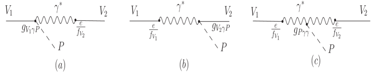
Figure 2: Schematic diagrams for $J/\psi(\psi^{\prime})\to\gamma^{*}\to VP$.

References

- [1] S.J. Brodsky and G.P. Lepage, Phys. Rev. D 24, 2848 (1981).
- [2] W. M. Yao et al. [Particle Data Group], J. Phys. G 33 1 (2006).
- [3] W.S. Hou and A. Soni, Phys. Rev. Lett. 50, 569 (1983).
- [4] G. Karl and W. Roberts, Phys. Lett. 144B, 263 (1984).
- [5] S.S. Pinsky, Phys. Rev. D 31, 1753 (1985).
- [6] S.J. Brodsky, G.P. Lepage and S.F. Tuan, Phys. Rev. Lett. 59, 621 (1987).
- [7] M. Chaichian and N.A. Törnqvist, Nucl. Phys. B 323, 75 (1989).
- [8] S.S. Pinsky, Phys. Lett. B 236, 479 (1990).
- [9] S.J. Brodsky and M. Karliner, Phys. Rev. Lett. 78, 4682 (1997).
- [10] X. Q. Li, D. V. Bugg and B. S. Zou, Phys. Rev. D 55, 1421 (1997).
- [11] Y.-Q. Chen and E. Braaten, Phys. Rev. Lett. 80, 5060 (1998).
- [12] J.-M. Gérald and J. Weyers, Phys. Lett. B 462, 324 (1999); P. Artoisenet, J.-M. Gérald and J. Weyers, Phys. Lett. B 628, 211 (2005).
- [13] T. Feldmann and P. Kroll, Phys. Rev. D 62, 074006 (2000).
- [14] M. Suzuki, Phys. Rev. D 63, 054021 (2001).
- [15] J.L. Rosner, Phys. Rev. D 64, 094002 (2001).
- [16] P. Wang, C.Z. Yuan, X.H. Mo, Phys. Lett. B 574, 41 (2004).
- [17] X. Liu, X.Q. Zeng and X.Q. Li, Phys. Rev. D 74, 074003 (2006) [arXiv:hep-ph/0606191].
- [18] X.H. Mo, C.Z. Yuan, and X.H. Mo, hep-ph/0611214.
- [19] Q. Zhao, G. Li and C. H. Chang, Phys. Lett. B 645, 173 (2007) [arXiv: hep-ph/0610223].
- [20] A. Seiden, H. F.-W. Sadrozinski and H.E. Haber, Phys. Rev. D 38, 824 (1988).
- [21] M. Ablikim et al. [BES Collaboration], Phys. Rev. D 71, 032003 (2005).
- [22] M. Ablikim et al. [BES Collaboration], Phys. Rev. D 70, 112007 (2004); Erratum-ibid, D71, 019901 (2005).
- [23] M. Ablikim et al. [BES Collaboration], Phys. Rev. D 70, 112003 (2004).
- [24] M. Ablikim et al. [BES Collaboration], Phys. Lett. B 614, 37 (2005).
- [25] H. Fritzsch and J.D. Jackson, Phys. Lett. 66B, 365 (1977).
- [26] E. Witten, Nucl. Phys. B149, 285 (1979).
- [27] F.J. Gilman and R. Kauffman, Phys. Rev. D 36, 2761 (1987).
- [28] N. Isgur, Phys. Rev. D 13, 122 (1976).
- [29] K. Kawarabayashi and N. Ohta, Nucl. Phys. B 175, 477 (1980).
- [30] Kuang-Ta Chao, Nucl. Phys. B 317 597 (1989).
- [31] J. Schechter, A. Subbaraman and H. Weigel, Phys. Rev. D 48, 339 (1993).
- [32] H. Leutwyler, Nucl. Proc. Suppl. 64 223 (1998); H. Leutwyler, Eur. Phys. J. C 17, 623 (2000).
- [33] T. Feldmann, P. Kroll, and B. Stech, Phys. Rev. D 58, 114006 (1998); Phys. Lett. B 449, 339 (1999); T. Feldmann, Int. J. Mod. Phys. A 15, 159 (2000); T. Feldmann, P. Kroll, Phys. Scripta T99 13 (2002)
- [34] P. Kroll, AIP Conf. Proc. 717, 451 (2004).
- [35] C. Morningstar and M. Peardon, Phys. Rev. D 56, 4043 (1997); Phys. Rev. D60, 034509 (1999); G. Bali et al., UKQCD Collaboration, Phys. Lett. B 309, 378 (1993); Y. Chen et al., Phys. Rev. D 73, 014516 (2005).
- [36] F.E. Close, G.R. Farrar and Z. Li, Phys. Rev. D 55, 5749 (1997).
- [37] G.R. Farrar, Phys. Rev. Lett. 76, 4111 (1996).
- [38] M.B. Cakir and G.R. Farrar, Phys. Rev. D 50, 3268 (1994).
- [39] L. Faddeev, A. J. Niemi and U. Wiedner, Phys. Rev. D 70, 114033 (2004) [arXiv:hep-ph/0308240].
- [40] D.-M. Li, H. Yu and S.-S. Fang, Eur. Phys. J. C 28, 335 (2003).
- [41] Q. Zhao, Phys.Rev. D72, 074001 (2005).
- [42] F. E. Close and Q. Zhao, Phys. Rev. D 71, 094022 (2005).
- [43] C. Amsler and F. E. Close, Phys. Lett. B 353, 383 (1995); Phys. Rev. D 53, 295 (1996)
- [44] F. E. Close and A. Kirk, Phys. Lett. B 483, 345 (2000).
- [45] S. Narison, Nucl. Phys. B 509, 312 (1998).
- [46] M. Ablikim et al. [BES Collaboration], Phys. Rev. Lett. 95, 262001 (2005).
- [47] Z. Bai et al. [Mark III Collaboration], Phys. Rev. Lett. 65, 2507 (1990).
- [48] T. Bolton et al. [Mark III Collaboration], Phys. Rev. Lett. 69, 1328 (1992).
- [49] J.E. Augustin et al. [DM2 Collaboration], Phys. Rev. D 46, 1951 (1992).
- [50] A. Falvard et al., Phys. Rev. D 38, 2706 (1988).
- [51] J.J. Becker et al., Phys. Rev. Lett. 59, 186 (1987).
- [52] T. Barnes, F.E. Close, P.R. Page and E.S. Swanson, Phys. Rev. D 55, 4157 (1997).
- [53] M. Acciarri et al. [L3 Collaboration], Phys. Lett. B 501, 1 (2001).
- [54] J.Z. Bai et al. [BES Collaboration], Phys. Rev. Lett. 91, 022001 (2003).
- [55] G. S. Huang [CLEO Collaboration], AIP Conf. Proc. 842, 616 (2006).