Lepton flavor violating signals of a little Higgs model at the high energy linear colliders
Chong-Xing Yue and Shuang Zhao
Department of Physics, Liaoning Normal University, Dalian
116029, China
E-mail:cxyue@lnnu.edu.cn
Abstract
Littlest Higgs model predicts the existence of
the doubly charged scalars , which generally have
large flavor changing couplings to leptons. We calculate the
contributions of to the lepton flavor violating
processes and
, and compare our numerical
results with the current experimental upper limits on these
processes. We find that some of these processes can give severe
constraints on the coupling constant and the mass parameter
. Taking into account the constraints on these free
parameters, we further discuss the possible lepton flavor violating
signals of at the high energy linear
collider experiments. Our numerical results show that the
possible signals of might be detected via the
subprocesses in the
future experiments.
I. Introduction
It is well known that the individual lepton numbers
, and are automatically conserved and the
tree level lepton flavor violating processes are absent in
the standard model . However, the neutrino oscillation
experiments have made one believe that neutrinos are massive,
oscillate in flavors, which presently provide the only experimental
hints of new physics and imply that the separated lepton numbers are
not conserved[1]. Thus, the requires some modification to
account for the pattern of neutrino mixing, in which the
processes are allowed. The observation of the signals in
present or future high energy experiments would be a clear signature
of new physics beyond the .
Some of popular specific models beyond the generally predict
the presence of new particles, such as new gauge bosons and new
scalars, which can naturally lead to the tree level coupling.
In general, these new particles could enhance branching ratios for
some processes and perhaps bring them into the observable
threshold of the present and next generations of collider
experiments. Furthermore, nonobservability of these processes
can lead to strong constraints on the free parameters of new
physics. Thus, studying the possible signals of new physics
in various high energy collider experiments is very interesting and
needed.
Little Higgs models[2] employ an extended set of global and gauge
symmetries in order to avoid the one-loop quadratic divergences and
thus provide a new method to solve the hierarchy between the
scale of possible new physics and the electroweak scale . In this kind of models, the Higgs boson is a
pseudo-Goldstone boson of a global symmetry which is spontaneously
broken at some high scales. Electroweak symmetry breaking
is induced by radiative corrections leading to a Coleman-Weinberg
type of potential. Quadratic divergence cancellation of radiative
corrections to the Higgs boson mass are due to contributions from
new particles with the same spin as the particles. This type
of models can be regarded as one of the important candidates of the
new physics beyond the .
The littlest Higgs model [3] is one of the simplest and
phenomenologically viable models, which realizes the little Higgs
idea. Recently, using of the fact that the model contains a
complex triplet Higgs boson , Refs.[4,5,6] have discussed the
possibility to introduce lepton number violating interactions and generation
of neutrino mass in the little Higgs scenario. Ref.[5] has shown
that most satisfactory way of incorporating neutrino masses is to
include a lepton number violating interaction between the triplet
scalars and lepton doublets. The tree level neutrino masses are
mainly generated by the vacuum expectation value of
the complex triplet , which does not affect the cancellation
of quadratic divergences in the Higgs mass. The neutrino masses can
be given by the term , in which ( are
generation indices) is the Yukawa coupling constant. As long as the
triplet is restricted to be extremely small, the value
of is of natural order one, i.e. 1, which
might produce large contributions to some of processes[6,7].
The aim of this paper is to study the contributions of the
couplings predicted by the model to the processes and and compare our
numerical results with the present experimental bounds on these
processes, and see whether the constraints on the free
parameter can be obtained. We further calculate
the contributions of the model to the processes
and ( or ) ,
and discuss the possibility of detecting the
signals of the model via these processes in the future
high energy linear collider experiments.
This paper is organized as follows. Section II contains a short
summary of the relevant couplings of the scalars (doubly
charged scalar , charged scalars , and
neutral scalar ) to lepton doublets. The contributions of
these couplings to the processes and are calculated
in section III. Using the current experimental upper limits on these
processes, we try to give the constraints on the coupling constant
in this section. Section IV is devoted to the computation
of the production cross sections of the processes
and induced by the doubly charged scalars
. Some phenomenological analyses are also included in this section. Our
conclusions are given in section V.
II. The couplings of the triplet scalars
The model[3] consists of a nonlinear
model with a global symmetry and a locally gauged symmetry
. The global symmetry is broken
down to its subgroup at a scale , which results
in 14 Goldstone bosons . Four of these are eaten by
the gauge bosons , resulting from the
breaking of , giving them masses. The Higgs
boson remains as a light pseudo Goldstone boson and other
give masses to the gauge bosons and form a scalar triplet
. The complex triplet offers a chance to introduce
lepton number violating interactions in the theory.
In the context of the model, the lepton number violating
interaction which is invariant under the full gauge group, can be
written as[5,7]:
(1)
Where and are generation indices, and (= 1,
2) are indices, and is a left handed
lepton doublet. is the Yukawa coupling constant and is
the charge-conjugation operator. Because of non-linear nature of
, this interaction can give rise to a
mass matrix for the neutrinos as:
(2)
One can see from Eq.(2) that, if we would like to stabilize the
Higgs mass and at the same time ensure neutrino masses consistent
with experimental data[8], the coupling constant must be of
order , which is unnaturally small. However, it has been
shown[4,5] that the lepton number violating interaction only
involving the complex scalar triplet can give a neutrino mass
matrix . Considering the current bounds on the
neutrino mass[8], there should be:
(3)
Thus, the coupling constant can naturally be of order one
or at least not be unnaturally small provided the of
the triplet scalar is restricted to be extremely small.
In this scenario, the triplet scalar has the couplings
to the left handed lepton pairs, which can be written as[5]:
(4)
Considering these couplings, Ref.[5] has investigated the
decays of the scalars and , and found
that the most striking signature comes from the doubly charged
scalars . The constraints on the coupling constant
and the triplet scalar mass parameter coming
from the muon anomalous magnetic moment and the
process are studied in
Ref.[7]. In the next section, we will calculate the contributions of
the charged scalars and to the
processes and .
III. The charged scalars and the processes and
Decay Process
Current limit
Bound
[10]
—–
[12]
—–
[13]
—–
[11]
[14]
[14]
[14]
Table 1: The current experimental upper limits on the
branching ratios of some processes and the
corresponding upper constraints on the free parameters.
The observation of neutrino oscillations[1] implies that the
individual lepton numbers are violated, suggesting
the appearance of the processes, such as and . The branching
ratios of these processes are extremely small in the with
right handed neutrinos. For example, Ref.[9] has shown . Such small branching ratio is
unobservable.
The present experimental upper limits on the branching ratios
[10], [11],
[12], [13], and [14] are
given in Table 1. Future experiments with increased sensitivity can
reduce these current limits by a few orders of magnitude(see,
e.g.[15]). In this section, we will use these data to give the
constraints on the free parameters and .
Figure 1: Feynman diagrams contributing to the radiative decay
due to the charged scalars .
The couplings of the charged scalars and
given in Eq.(4) can lead to the radiative decays
at the one loop level
mediated by the exchange of the charged scalars and
, as shown in Fig.1. For the doubly charged scalar
, the photon can be attached either to the internal
lepton line or to the scalar line. For the charged scalar
, the photon can be only attached to the scalar line[16].
Using Eq.(4), the expression of the branching ratio
can be written as at
leading order:
(5)
Where is the fine structure constant and is the
Fermi constant. The factor means that, when the
internal lepton is the same as one of the leptons and
, the contributions of to
is four times those for
and . and are the
masses of the scalars and , respectively. In
the model, the scalar mass is generated through the
Coleman-Weinberg mechanism and the scalars ,
and degenerate at the lowest order[5]. Thus, we can
assume and write the branching ratio
as:
(6)
In particular, for the decay process , we obtain the following expression for the branching
ratio :
(7)
Figure 2: The coupling constant as a function of the scalar mass
for different values of the coupling constant .
From above equations, we can see that the process
can not be able to constrain
independently. However, if we assume for ( is
the flavor-diagonal coupling constant) and for
( is the flavor-mixing coupling constant), then
we can obtain the constraints on the combination of the free
parameters , and . Observably, the most stringent
constraint should come from the current experimental upper limits on
the branching ratio . Thus, in Fig.2, we
have shown the coupling constant as a function of the mass
parameter for , and
. From Fig.2, one can see the upper limit on
strongly depend on the values of and . For
and , there must be
.
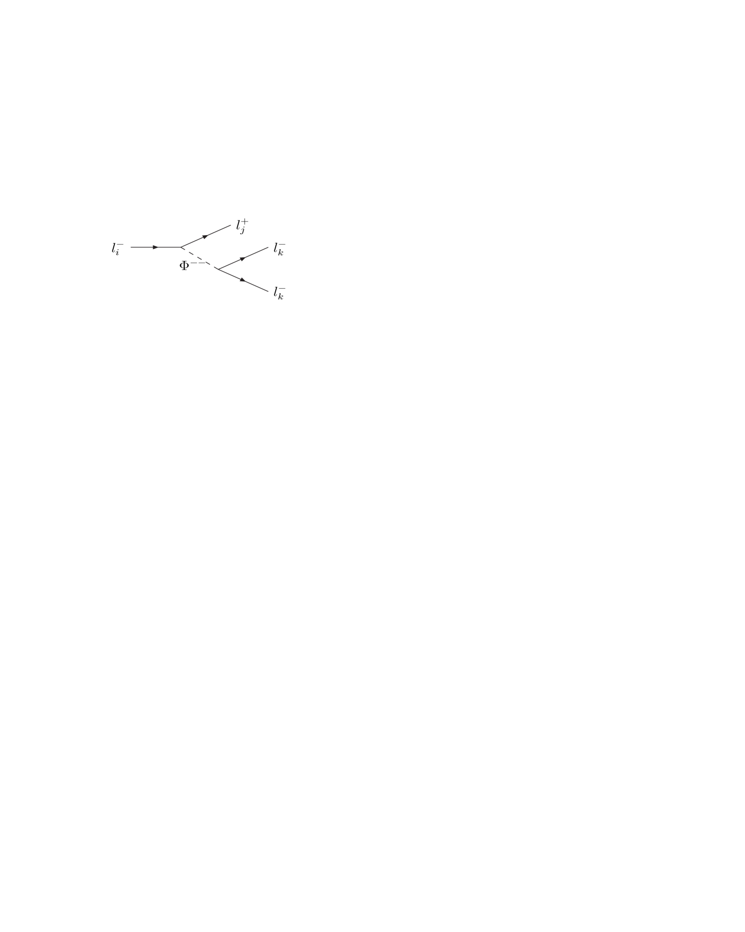
In the model, the processes can be generated at tree level through the exchange
of doubly charged scalar , as depicted in Fig.3.
Figure 3: Tree level Feynman diagram for the processes mediated by the doubly charged scalar .
The expressions of the branching ratios for the processes
are given
by[16,17]
(8)
(9)
(10)
(11)
(12)
Certainly, up to one loop, the processes get additional contributions from the processes
.
Thus, the charged scalars and have
contributions to the processes at one loop. However, compared with the tree level
contributions, they are very small, which can be safely neglected.
The processes also can not
give the constraints on the coupling constants
independently, but would be able to constrain the combination . Our numerical results are
given in Table 1.
In the following section, we will take into account these
constraints coming from the processes and , estimate the
contributions of the doubly charged scalars to the
processes and
, and discuss the
possibility of detecting the signals for the doubly charged scalars
at the experiments.
IV. The doubly charged scalars and the
processes
and
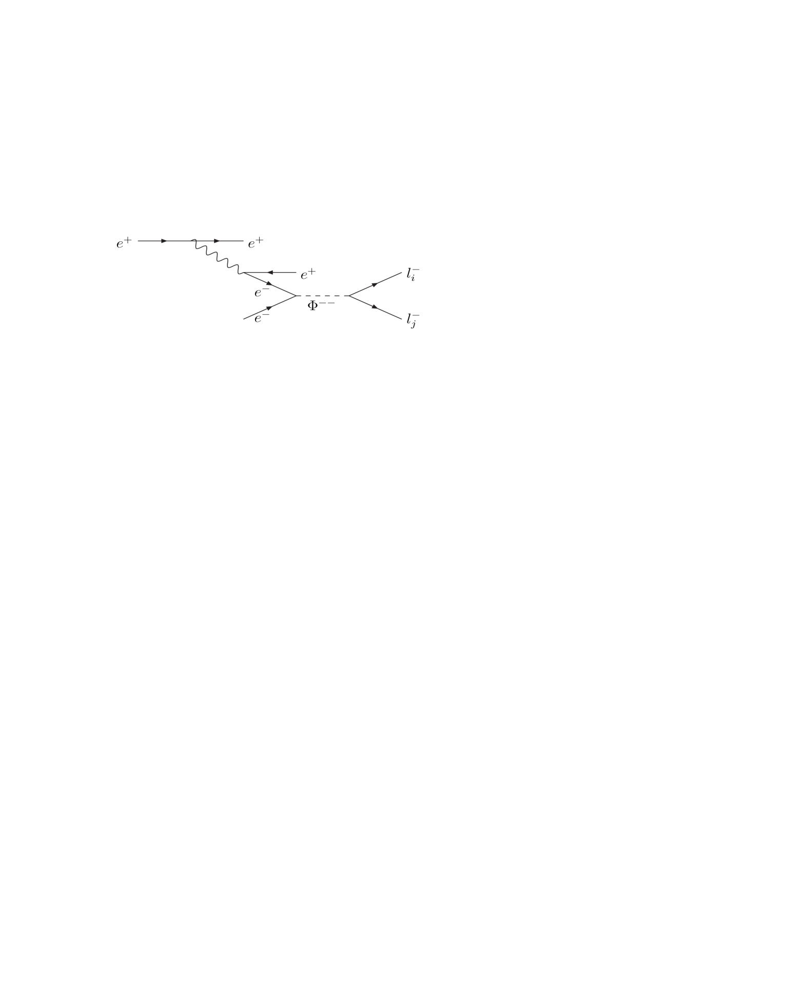
Figure 4: Main Feynman diagram for the processes
predicted by .
In general, the doubly charged scalars can not couple to quarks and
their couplings to leptons break the lepton number by two units,
leading to a distinct signature, namely a pair of same sign leptons.
The discovery of a doubly charged scalar would have important
implications for our understanding of the Higgs sector and more
importantly, for what lies beyond the . This fact has made one
give more elaborate theoretical calculations in the framework of
some specific models beyond the and see whether the signatures
of this kind of new particles can be detected in the future high
energy experiments. For example, the production and decay of the
doubly charged scalars and their possible signals at the have
been extensively studied in Refs.[18,19]. In this section, we will
consider the contributions of the doubly charged scalars
predicted by the model to the processes
and
( or
). The processes can be seen as the subprocesses of the
processes . For
example, the doubly charged scalar generates contributes
to the process through
the subprocess , as shown
in Fig.4.
Using Eq.(4), the expression of the cross section for the subprocess
can be easily written as:
(13)
Where is the center-of-mass energy of
the subprocess .
is the total decay width of the doubly charged
scalar , which has been given by Ref.[5] in the case of
the triplet scalars and
degenerating at lowest order with a common mass :
(14)
Where is the coupling constant,
is the coupling constant. In above equation, the
final-state masses have been neglected compared to the mass
parameter . It has been shown that, for , the main decay modes of are
. Furthermore, the FX coupling constant are
subject to very stringent bounds from the process
. In this case, the decay width
can be approximately written as:
(15)
Considering the current bounds on the neutrino mass[8], there should
be:
(16)
so leads to , which
does not conflict with the most stringent constraint from the
process . Thus, in our numerical calculation, we
will take Eq.(15) as the total decay width of .
Using the equivalent particle approximation method[20], the
effective cross section for the process can be approximately written as[19]:
(17)
Where and .
is the equivalent electron
distribution function of the initial positron, which gives the
probability that an electron with energy is
emitted from a positron beam with energy . The relevant
expression can be written as[21]:
(18)
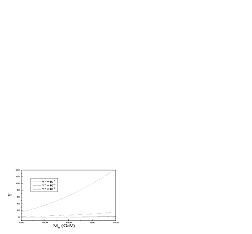
In Fig.5 and Fig.6, we plot the production cross
sections and for the
processes and
as function of the FD
coupling constant , respectively. In these figures, we have
assumed and taken and
. From Fig.5 and Fig.6 one can see
that the values of and
are strongly depend on the value of the coupling constant
. For and , the values of
the subprocess cross section and the
effective cross section are larger than fb and fb, respectively.
The signal of the doubly charged scalar given by the
process is so distinctive and
is the background free, discovery would be signalled by even
few events. In Fig.7, we plot the discovery region in the
plane at 95% confidence level for seeing 5
events, in which we have assumed the future
with the energy and the yearly integrated
luminosity of [22]. From this figure, one
can see that, in wide range of the parameter space, the signals of
should be detected in the future ILC experiments.
The doubly charged scalar can also has
contributions to the processes
and
. However, the experimental upper limits on the
processes , , and
can give severe constraints on the combination
, which makes the
production cross sections of these processes very small. For
example, even if we take and , the
production cross sections , and
are smaller than fb, fb, and fb, respectively. Thus, it is
very difficult to detect the signals of via the
processes in the
future experiments.
Certainly, the doubly charged scalar has contributions
to the processes and
. Similar with above
calculation, we can give the values of the production cross sections
for these processes. We find that the cross section
is equal to the cross section
. Thus, the conclusions for the doubly
charged scalar are also apply to the doubly charged
scalar .
V. Conclusions
To solve the so-called hierarchy or fine tuning problem
of the , the little Higgs theory was proposed as a kind of
models to accomplished by a naturally light Higgs boson. The
model is one of the simplest and phenomenologically viable
models. In the model, neutrino masses and mixings can be
generated by coupling the scalar triplet to the leptons in a
interaction, whose magnitude is proportional to
the triplet multiplied by the Yukawa coupling constant
without invoking a right handed neutrino. This scenario
predicts the existence of doubly charged scalars .
For smaller values of i.e. , the
doubly charged scalars have large flavor changing
coupling to leptons, which can generate significantly contributions
to some processes and give characteristic signatures in the
future high energy experiments.
In this paper, we first consider the processes
and in the context of the model. For the
process , it involves all of the FX
coupling constants , we can not give the simple
constraints about the free parameters and . Thus,
for the fixed values of the FX coupling constant , we take into account the current experimental upper limit of
the and plot the FD coupling constant
as a function of the mass parameter . Our
numerical results show that the upper limit on is strongly
depend on the free parameters and .
Using the present experimental upper limits on the branching ratios
, we obtain the constraints on
the combination . We
find that the most stringent constraint comes from the process
. In all of the parameter space, there must be
.
The characteristic signals of the processes is same-sign dileptons or two same-sign
different flavor leptons, which is the background free and
offers excellent potential for doubly charged scalar discovery. To
see whether the doubly charged scalar can be detected in
the future experiments, we discuss the contributions of
to the processes and .
We find that the triplet scalar can give significantly
contributions to the processes . In wide range of the parameter space of the
model, the possible signals of might be observed in
the future experiments. However, the production cross sections
of the processes mediated by are very small.
The contributions of the triplet scalar to the processes
are equal to those of
for the processes , Thus, our conclusions are also apply to the
doubly charged scalar .
Some popular models beyond the predict the existence of doubly
charged scalars, which generally have the lepton number and lepton
flavor changing couplings to leptons and might produce distinct
experimental signatures in the current or future high energy
experiments. Their observation would signal physics outside the
current paradigm and further test the new physics models. Search for
this kind of new particles has been one of the important goals of
the high energy experiments[23]. Thus, the possibly signals of the
doubly charged scalars predicted by the little Higgs
models should be more studied in the future.
Acknowledgments
This work was supported in part by Program for New Century Excellent
Talents in University(NCET-04-0290), the National Natural Science
Foundation of China under the Grants No.10475037 and 10675057.
References
[1]
M. C. Gonzalez-Garcia and Y. Nir, Rev. Mod. Phys.75, 345(2003); V. Barger, D. Marfatia, and K. Whisnant, Int. J. Mod. Phys E12,
569(2003); A. Y. Smimov, hep-ph/0402264.
[2]
For recent review see: M. Schmaltz and D. Tucker-Smith, Ann.
Rev. Nucl. Parti. Sci. 55, 229(2005); T. Han, H. E.
Logan, and L. T. Wang, JHEP0601, 099(2006).
[3]
N. Arkani-Hamed, A. G. Cohen, E. Katz, A. E. Nelson, JHEP0207, 034(2002).
[4]
W. Kilian and J. Reuter, Phys. Rev.
D70, 015004(2004); J. Y. Lee, JHEP 0506, 060(2005).
[5]
T. Han, H. E. Logan, B. Mukhopadhyaya and R. Srikanth, Phys.
Rev. D72, 053007(2005).
[6]
A. Goyal, hep-ph/0506131
[7]
S. R. Choudhury, N. Gaur, and A. Goyal, Phys. Rev. D72, 097702(2005).
[8]
G. L. Fogli et al, Phys. Rev. D70,
113003(2004); M. Tegmark et al. [SDSS Collaboration], Phys. Rev. D69,
103501(2004); O. Elgaroy and O. Lahav, New J. Phys. 7, 61(2005)
[9]
S. M. Bilenky, S. T. Petcov, and B. Pontecorvo, Phys. Lett. B67, 309(1977); T. P. Cheng and L. F. Li, Phys. Rev. Lett.45,
1908(1980).
[10]
M. L. Brooks et al. [MEGA Collaboration], Phys. Rev. Lett.83,
1521(1999).
[11]
U. Bellgardt et al. [SINDRUM Collaboration], Nucl. Phys. B299,
1(1988).
[12]
B. Aubert et al. [BABAR Collaboration], Phys. Rev. Lett.96,
041801(2006).
[13]
B. Aubert et al. [BABAR Collaboration], Phys. Rev. Lett.95,
041802(2005).
[14]
B. Aubert et al. [BABAR Collaboration], Phys. Rev. Lett.92,
121801(2004).
[15]
Y. Kuno and Y. Okada, Rev. Mod. Phys.73, 151(2001).
[16]
R. N. Mohapatra, Phys. Rev. D46,
2990(1992); F. Cuypers, S. Davidson, Eur. Phys. J. C2,
503(1998).
[17]
M. L. Swartz, Phys. Rev. D40,
1521(1989).
[18]
G. Barenboim, K. Huitu, J. Maalampi, M. Raidal, Phys. Lett. B394, 132(1997); F. Cuypers, S. Davidson, Eur. Phys. J. C2,
503(1998); A. G. Akeroyd, M. Aoki, Phys. Rev.
D72, 035011(2005); A. G. Akeroyd, Y. Okada, hep-ph/0610344.
[19]
E. M. Gregores, A. Gusso, S. F. Novaes, Phys. Rev.
D64,
015004(2001); S. Godfrey, P. Kalyniak, N. Romanenko, Phys. Lett. B545, 361(2002); S. Atag and K. O. Ozansoy, Phys. Rev. D70,
053001(2004).
[20]
V. N. Baier, V. S. Fadin, and V. A. Khoze, Nucl. Phys. B65,
381(1973); M.-S. Chen and P. Zerwas, Phys. Rev. D12,
187(1975); I. F. Ginzburg and V. G. Serbo, Phys. Rev. D49,
2623(1994).
[21]
T. Sjostrand, Comput. Phys. Commun. 82,
74(1994).
[22]
T. Abe et al. [American Linear Collider Group], hep-ex/0106057;
J. A. Aguilar-Saavedra et al.
[ECFA/DESY LC Physics Working Group], hep-ph/0106315; K. Abe et al. [ACFA Linear Collider Working Group],
hep-ph/0109166; G. Laow et al.,
ILC Techinical Review Committee, second report, 2003,
SLAC-R-606.
[23]
P. Achard et al. [L3 Collaboration], Phys. Lett. B576, 18(2003); G. Abbiendi et al. [OPAL Collaboration], Phys. Lett. B577, 93(2003); J. Abdallah et al. [DELPHI Collaboration], Phys. Lett. B552, 127(2003); D. Acosta et al. [CDF Collaboration], Phys. Rev. Lett.93,
221802(2004); V. M. Abazov et al. [D0 Collaboration], Phys. Rev. Lett.93,
141801(2004).

![[Uncaptioned image]](/html/hep-ph/0701017/assets/x5.png)
![[Uncaptioned image]](/html/hep-ph/0701017/assets/x7.png)