Cavity tests of parity-odd Lorentz violations in electrodynamics

Abstract

Electromagnetic resonant cavities form the basis for a number modern tests of Lorentz invariance. The geometry of most of these experiments implies unsuppressed sensitivities to parity-even Lorentz violations only. Parity-odd violations typically enter through suppressed boost effects, causing a reduction in sensitivity by roughly four orders of magnitude. Here we discuss possible techniques for achieving unsuppressed sensitivities to parity-odd violations by using asymmetric resonators.

I introduction

In recent years, renewed interest in precision tests of relativity has resulted in a number of modern version of the classic Michelson-Morley mm and Kennedy-Thorndike kt experiments cavities . These tests are motivated in part by the observation that attempts to quantize gravity may lead to tiny violations of Lorentz invariance at attainable energies. While originally conceived within the context of spontaneous symmetry breaking in string theory ks ; kp , a number of other possible origins have been proposed ncqed ; qg ; fn ; bj . Remarkably, naive estimates suggest that these violations may be within reach of contemporary experiment cpt ; ck ; kost .

Lorentz invariance includes covariance under both rotations and boosts. Traditionally, Michelson-Morley-type experiments test the rotational invariance, while Kennedy-Thorndike experiments focus on boost symmetry. Modern versions are normally sensitive to both types of violations, but sensitivities to boost effects are usually suppressed relative to rotational violations due to the small velocities involved in most experiments. The symmetry of most resonators imply that only parity-even violations of Lorentz invariance are observable in Michelson-Morley tests and are detectable at unsuppressed levels. Parity-breaking and isotropic Lorentz violations enter at first and second order in small velocities, causing reduced sensitivities.

While sensitivities to Lorentz violations in photons continue to improve, a substantial increase in sensitivity to parity-odd violations may be possible in experiments that do not respect parity symmetry. In this work, we focus on resonator experiments, exploring the reasons behind the suppression and the potential for parity-asymmetric resonators to yield higher sensitivities to parity-odd Lorentz violations. Other suggestions for improving sensitivity to parity-odd violations include searches for mixing between the electric-field vector and the magnetic-field pseudovector in electromagnetostatic experiments kb and the use of interferometers or traveling-wave resonators tobar .

General violations of Lorentz invariance are described by a field-theoretic framework known as the Standard-Model Extension (SME) ck ; kost . The SME provides a systematic theoretical basis for studies of Lorentz invariance in many systems, including those involving photons cavities ; km ; tobar ; kb ; km-bire ; cfj ; photonth ; sher , baryons ccexpt ; spaceexpt , hadrons hadrons ; hadronth , electrons electrons ; electronth , muons muons , neutrinos neutrinos , Higgs bosons higgs , and gravitation kb-gr ; kp2 . Here we work within the renormalizable gauge-invariant $CPT$-even photon sector of the minimal SME, but many of the symmetry arguments presented here may be extended to more general violations.

The structure of this paper is as follows. Section II.1 gives a review of the theory and notation used in this paper. The general theory behind resonator experiments is described in Sec. II.2. The possibility of using resonators with parity-breaking geometries is discussed in Sec. III. Section IV presents a numerical example of a parity-asymmetric resonant cavity. Some concluding remarks are given in Sec. V.

II basic theory

This section provides some basic theory and definitions. Lorentz violation in the photon sector of the minimal SME is reviewed, and the characterization of potential sensitivities in general resonator experiments is given.

II.1 Framework

The violations of interest are described by a modified Maxwell lagrangian ck ,

$${\cal L}=-\frac{1}{4}F^{\mu\nu}F_{\mu\nu}-\frac{1}{4}(k_{F})^{\kappa\lambda\mu\nu}F_{\kappa\lambda}F_{\mu\nu}\ ,$$ (1)

where tensor coefficients $(k_{F})^{\kappa\lambda\mu\nu}$ characterize the extent to which Lorentz symmetry is violated. The tensor $(k_{F})^{\kappa\lambda\mu\nu}$ is real and obeys the symmetries of the Riemann tensor. In addition, the double trace is usually assumed to be zero since it only contributes to a scaling of the theory. This leaves a total of 19 independent coefficients for Lorentz violation. These coefficients are taken to be constant in the minimal SME, but may depend on spacetime location in more general contexts, including those involving gravitation kost ; kp2 ; kb-gr . Other forms of Lorentz violation that could also be considered include the $CPT$-odd $k_{AF}$ term of the minimal SME ck , and nonrenormalizable terms of the general SME kpo ; kle .

The equations of motion associated with lagrangian (1) provide modified inhomogeneous Maxwell equations. It turns out that these can be cast into the familiar form $\mbox{\boldmath$\nabla$}\times\mbox{\boldmath$H$}-\partial_{0}\mbox{\boldmath$D$}=0$, $\mbox{\boldmath$\nabla$}\cdot\mbox{\boldmath$D$}=0$, provided we define km

$$\mbox{\boldmath$D$}=\ (\epsilon_{DE}+\kappa_{DE})\cdot\mbox{\boldmath$E$}+(\epsilon_{DB}+\kappa_{DB})\cdot\mbox{\boldmath$B$}\ ,$$

$$\mbox{\boldmath$H$}=\ (\epsilon_{HE}+\kappa_{HE})\cdot\mbox{\boldmath$E$}+(\epsilon_{HB}+\kappa_{HB})\cdot\mbox{\boldmath$B$}\ .$$ (2)

Here we allow for the possibility of general linear passive magnetoelectric media with constituent matrices $\epsilon_{DE}$, $\epsilon_{DB}$, $\epsilon_{HE}$, and $\epsilon_{HB}$ kong . For harmonic fields, these matrices are complex and may depend on frequency. Losslessness implies that $\epsilon_{DE}$ and $\epsilon_{DB}$ are hermitian and $\epsilon_{HE}=-\epsilon_{DB}^{\dagger}$. In many applications these reduce to a simple isotropic permittivity and permeability: $\epsilon_{DE}=\epsilon$, $\epsilon_{HB}=\mu^{-1}$, and $\epsilon_{DB}=\epsilon_{HE}=0$.

In this language, Lorentz violation in photons is controlled by the real $3\times 3$ matrices $\kappa_{DE}$, $\kappa_{DB}$, $\kappa_{HE}$, and $\kappa_{HB}$, which result from a 1-3 decomposition of the $(k_{F})^{\kappa\lambda\mu\nu}$ tensor. These matrices obey the same lossless conditions as their $\epsilon$ counterparts. Note that $\kappa_{DE}$ and $\kappa_{HB}$ are parity conserving, while $\kappa_{DB}=-\kappa_{HE}^{T}$ mixes vectors and pseudovectors, introducing parity violations. Also note that it is usually assumed that the $\epsilon$ matrices are not significantly altered by Lorentz violation in photons.

A subset of the coefficients for Lorentz violation cause vacuum birefringence, which can be tested with extreme precision by polarimetry of light from sources at cosmological distances cfj ; km-bire ; km . It is therefore useful to decompose the $\kappa$ matrices into coefficients that cause birefringence and those that do not:

$$\kappa_{DE} =\tilde{\kappa}_{e+}+\tilde{\kappa}_{e-}+\tilde{\kappa}_{\rm tr}\ ,$$

$$\kappa_{HB} =\tilde{\kappa}_{e+}-\tilde{\kappa}_{e-}-\tilde{\kappa}_{\rm tr}\ ,$$ (3)

$$\kappa_{DB} =-\kappa_{HE}^{T}=\tilde{\kappa}_{o+}+\tilde{\kappa}_{o-}\ .$$

Here $\tilde{\kappa}_{e+}$, $\tilde{\kappa}_{e-}$, $\tilde{\kappa}_{o+}$, and $\tilde{\kappa}_{o-}$ are $3\times 3$ real traceless matrices. The matrix $\tilde{\kappa}_{o+}$ is antisymmetric, and the other three are symmetric. The remaining trace component $\tilde{\kappa}_{\rm tr}$ represents a single real coefficient and is associated with isotropic violations.

The coefficients in $\tilde{\kappa}_{e-}$, $\tilde{\kappa}_{o+}$, and $\tilde{\kappa}_{\rm tr}$ mimic a small distortion in the spacetime metric, resulting in a distorted version of the usual electrodynamics. In contrast, the coefficients $\tilde{\kappa}_{e+}$ and $\tilde{\kappa}_{o-}$ break the usual two-fold degeneracy that occurs in electrodynamics, causing light to propagate as the superposition of two modes that differ in speed and polarization. This causes birefringence and results in a change in the net polarization of light as it propagates. Searches for birefringence in light from astrophysical sources have resulted in stringent constraints at the level of $10^{-32}$ or less on the 10 coefficients in $\tilde{\kappa}_{e+}$ and $\tilde{\kappa}_{o-}$ km-bire . Consequently, resonator experiments normally focus on the 8 coefficients in $\tilde{\kappa}_{o+}$ and $\tilde{\kappa}_{e-}$, which do not cause birefringence. The isotropic coefficient $\tilde{\kappa}_{\rm tr}$ is not usually considered because it is doubly suppressed. However, in principle, resonator experiments can test all 19 coefficients.

II.2 Resonator experiments

Equation (2) suggests that the effects of Lorentz violation are similar to those of linear media. This analogy provides an intuitive understanding of the basic principle behind resonant-cavity experiments. The matter effects from the $\epsilon$ matrices generally depend on the orientation of the media within the cavity. However, since the location and orientation of media are typically fixed with respect to the apparatus, the frequency does not change with changes in the orientation or velocity of the resonator. In contrast, the $\kappa$ matrices can be viewed as constant background fields pervading all of space. The cavities are immersed in these background fields, and changing the orientation or velocity of the cavity with respect to these fields can lead to a change in resonant frequency.

To test for these effects, experiments search for small variations in resonant frequencies with changes in orientation or velocity. Rotations of the resonator are normally achieved through either the sidereal motion of the Earth or more actively through the use of turntables. Experiments monitor the frequency, searching for rotation-violating Michelson-Morley-type signals. To date, this method has yielded sensitivity to parity-even coefficients only. At present, $\tilde{\kappa}_{e-}$ is constrained at the level of $\sim 10^{-16}$ by Michelson-Morley techniques cavities .

Sensitivity to the parity-odd $\tilde{\kappa}_{o+}$ has only been obtained through Kennedy-Thorndike tests, resulting in less stringent constraints. The reason for this stems from the fact that frequency is a parity-even quantity. In parity-symmetric resonators, parity-odd violations can only affect the frequency if they contribute in conjunction with another parity-odd quantity. Boost effects allow for this since they involve a parity-odd velocity. As a result, Kennedy-Thorndike effects are usually suppressed by a factor of $\beta\sim 10^{-4}$, the typical velocity of the apparatus. Consequently, current constraints on parity-odd $\tilde{\kappa}_{o+}$ coefficients are near $10^{-12}$.

Similar symmetry arguments apply to the isotropic violations associated with $\tilde{\kappa}_{\rm tr}$. Isotropic effects are difficult to observable, but $\tilde{\kappa}_{\rm tr}$ does cause observable boost violations. However, arguments similar to those given above imply that these effects enter suppressed by two factors of velocity, giving a suppression factor of $\sim 10^{-8}$ in parity-symmetric experiments. While searching for these effects in resonators is feasible, current bounds on this coefficient use other techniques sher .

For resonators, the effects of Lorentz violation are characterized by the leading-order shifts in resonant frequencies, given by the generic expression

$${{\delta\nu}\over{\nu_{0}}}=\ ({\cal M}_{DE})^{jk}(\kappa_{DE})^{jk}+({\cal M}_{HB})^{jk}(\kappa_{HB})^{jk}$$

$$+({\cal M}_{DB})^{jk}(\kappa_{DB})^{jk}\ ,$$ (4)

where $({\cal M}_{DE})^{jk}$, $({\cal M}_{HB})^{jk}$, and $({\cal M}_{DB})^{jk}$ are experiment-dependent factors. Typically one begins an analysis by calculating these dimensionless factors in a frame that is fixed to the resonator. In this frame, the $\cal M$ matrices are experiment-specific numerical constants. In contrast, the $\kappa$ matrices are constant only in inertial frames. By convention, a standard Sun-centered inertial frame is used, and all measurements are reported in terms of coefficients in this frame. A coordinate transformation is used to relate the resonator-frame $\kappa$ matrices to constant Sun-frame matrices. This transformation introduces the orientation and velocity dependence that constitute the signals for Lorentz violation. Neglecting boost effects, the resonator-frame and Sun-frame $\kappa$’s are related by a rotation. This implies that the unsuppressed Michelson-Morley-type sensitivity to a particular Sun-frame $\kappa$ matrix is completely determined by the corresponding resonator-frame $\cal M$ matrix. For example, an experiment with nonzero ${\cal M}_{DB}$ would be sensitive to rotational effects associated with a nonzero $\kappa_{DB}$. In contrast, zero ${\cal M}_{DB}$ implies that only suppressed boost effects arise from nonzero $\kappa_{DB}$.

The $\cal M$ matrices can be calculated perturbatively in terms of the fields in the absence of Lorentz violation, $\mbox{\boldmath$E$}_{0}$, $\mbox{\boldmath$D$}_{0}$, $\mbox{\boldmath$B$}_{0}$, and $\mbox{\boldmath$H$}_{0}$ km :

$$({\cal M}_{DE})^{jk} =-\frac{1}{4U}\int d^{3}x\ {\rm Re}\ (E_{0}^{*})^{j}(E_{0})^{k}\ ,$$

$$({\cal M}_{HB})^{jk} =\phantom{-}\frac{1}{4U}\int d^{3}x\ {\rm Re}\ (B_{0}^{*})^{j}(B_{0})^{k}\ ,$$ (5)

$$({\cal M}_{DB})^{jk} =-\frac{1}{2U}\int d^{3}x\ {\rm Re}\ (E_{0}^{*})^{j}(B_{0})^{k}\ ,$$

where $U=\frac{1}{4}\int d^{3}x\ (\mbox{\boldmath$E$}_{0}^{*}\cdot\mbox{\boldmath$D$}_{0}+\mbox{\boldmath$B$}_{0}^{*}\cdot\mbox{\boldmath$H$}_{0})$ is the time-averaged energy stored in the resonator. In what follows, it will be useful to have a birefringent decomposition of these matrices,

$${\cal\widetilde{M}}_{e+} ={\cal M}_{DE}+{\cal M}_{HB}-{\textstyle{{1}\over{3}}}{\rm Tr}({\cal M}_{DE}+{\cal M}_{HB})\ ,$$

$${\cal\widetilde{M}}_{e-} ={\cal M}_{DE}-{\cal M}_{HB}-{\textstyle{{1}\over{3}}}{\rm Tr}({\cal M}_{DE}-{\cal M}_{HB})\ ,$$

$${\cal\widetilde{M}}_{o+} ={\textstyle{{1}\over{2}}}({\cal M}_{DB}-{\cal M}_{DB}^{T})\ ,$$ (6)

$${\cal\widetilde{M}}_{o-} ={\textstyle{{1}\over{2}}}({\cal M}_{DB}+{\cal M}_{DB}^{T})-{\textstyle{{1}\over{3}}}{\rm Tr}{\cal M}_{DB}\ ,$$

$${\cal\widetilde{M}}_{\rm tr}\ ={\rm Tr}({\cal M}_{DE}-{\cal M}_{HB})=-1\ .$$

These $\cal\widetilde{M}$ matrices characterize the dependence on the $\tilde{\kappa}$ matrices through an expression analogous to Eq. (4). Here we want to explore sensitivity to parity-odd violations, so our primary focus will be on ${\cal\widetilde{M}}_{o+}$ and ${\cal\widetilde{M}}_{o-}$ matrices.

Note that the $\cal\widetilde{M}$ matrices are calculated using conventional solutions. Therefore, to determine the effects of Lorentz violation on resonator frequencies, we need only to solve for the fields in the Lorentz-invariant case. Consequently, we drop the subscript 0 on all fields in what follows, with the understanding that we are working within the usual Lorentz-invariant electrodynamics, and all fields are conventional.

III parity-breaking resonators

Mathematically, the reason parity-odd Lorentz violations do not typically contribute at unsuppressed levels is because the solutions can be split into solutions of definite parity. In parity-symmetric cavities with parity-conserving media, the boundary conditions and the Maxwell equations normally admit conventional nondegenerate resonances of the form, $\mbox{\boldmath$E$}_{\pm}(\mbox{\boldmath$x$})=\pm\mbox{\boldmath$E$}_{\pm}(-\mbox{\boldmath$x$})$, $\mbox{\boldmath$B$}_{\pm}(\mbox{\boldmath$x$})=\mp\mbox{\boldmath$B$}_{\pm}(-\mbox{\boldmath$x$})$. The result is that ${\cal M}_{DB}$ in Eq. (5) vanishes, since $(E_{\pm}^{*})^{j}(\mbox{\boldmath$x$})(B_{\pm})^{k}(\mbox{\boldmath$x$})=-(E_{\pm}^{*})^{j}(-\mbox{\boldmath$x$})(B_{\pm})^{k}(-\mbox{\boldmath$x$})$. The result is a zero ${\cal M}_{DB}$, which implies no sensitivity to parity-odd Lorentz violations. So, in order to access parity-odd violations, we should construct resonators that admit solutions of indefinite parity.

Resonators could be constructed that break parity symmetry by using asymmetric geometries or by introducing parity-breaking media. Below we demonstrate this with an explicit example, but we first show that, in either case, one cannot achieve unsuppressed sensitivity to certain combinations of Lorentz violations using a single lossless resonator.

We begin by noting that the average flow of electromagnetic energy within a volume $V$ can be split into terms representing the energy flowing through the surface of $V$ and the energy from sources and sinks within $V$. The explicit expression, in terms of the harmonic Poynting vector $\mbox{\boldmath$S$}={\textstyle{1\over 2}}{\rm Re}\ \mbox{\boldmath$E$}^{*}\times\mbox{\boldmath$H$}$, is given by the integral identity

$$\int_{V}\mbox{\boldmath$S$}\ d^{3}x=\oint_{\partial V}\mbox{\boldmath$x$}\ \mbox{\boldmath$S$}\cdot d\mbox{\boldmath$a$}-\int_{V}\mbox{\boldmath$x$}\ \mbox{\boldmath$\nabla$}\!\cdot\mbox{\boldmath$S$}\ d^{3}x\ .$$ (7)

For harmonic fields, the source term vanishes since $\mbox{\boldmath$\nabla$}\!\cdot\mbox{\boldmath$S$}=0$ in regions without current jackson . This is simply the statement that there are no sources or sinks of energy within the resonator. This leaves the surface term and the energy flowing through $\partial V$. This term vanishes immediately if the fields are sufficiently confined to the interior of $V$. It also vanishes if we impose perfect-conductor boundary conditions at $\partial V$. In this case, $E$ is perpendicular to the surface $\partial V$, so $S$ is parallel to $\partial V$. This implies that, on average, no energy is exchanged with any portion of the conductor, and the average-energy-flow lines are confined to the volume of the cavity. Equation (7) then implies that $\int_{V}\mbox{\boldmath$S$}\ d^{3}x=0$. It follows that

$$\int_{V}{\rm Re}\ (\mbox{\boldmath$E$}^{*}\otimes\mbox{\boldmath$H$}-\mbox{\boldmath$H$}\otimes\mbox{\boldmath$E$}^{*})\ d^{3}x=0\ .$$ (8)

This $3\times 3$ antisymmetric matrix equation places three real constraints on the $\cal M$ matrices. This implies that, for a given lossless resonator, regardless of geometry, there are at least three combinations of coefficients for Lorentz violation that are inaccessible at unsuppressed levels.

As an example, consider a cavity filled with a frequency-independent medium. In this case, the $\epsilon$ constituent matrices are real, and the above discussion implies

$$2\,({\cal M}_{DE})\cdot(\epsilon_{DB})-2\,(\epsilon_{DB})^{T}\!\cdot({\cal M}_{DE})$$

$$-({\cal M}_{DB})\cdot(\epsilon_{HB})+(\epsilon_{HB})\cdot({\cal M}_{DB})^{T} =0\ ,$$ (9)

assuming the the constituent matrices $\epsilon_{HB}$ and $\epsilon_{DB}$ are uniform throughout the volume $V$. This matrix equation places three constraints on the $\cal M$ matrices, implying that three combinations of $\kappa$ matrices are inaccessible. A particularly relevant simple case is a cavity containing a simple magnetic medium with $\epsilon_{DB}=0$ and $\epsilon_{HB}=\mu^{-1}$, where $\mu$ is a homogeneous isotropic permeability. Equation (9) then implies that the antisymmetric component of ${\cal M}_{DB}$ vanishes. Consequently, ${\cal\widetilde{M}}_{o+}$ is zero and $\tilde{\kappa}_{o+}$ no longer contributes to the fractional frequency shift at unsuppressed levels. The conclusion is that resonators incorporating simple isotropic magnetic media have no sensitivity to nonbirefringent parity-odd violations. Sensitivity to the three components of $\tilde{\kappa}_{o+}$ can only be obtained by the introduction of more complicated magnetic materials. This is of particular interest because the 3 coefficients in $\tilde{\kappa}_{o+}$ are the least constrained of the 18 anisotropic coefficients for Lorentz violation.

IV numerical example

In this section, we give a numerical example of a resonant cavity with parity-breaking geometry. A numerical method for solving the Maxwell equations in curvilinear coordinates is given, and used to illustrate some of the conclusions of the previous section.

IV.1 Geometry

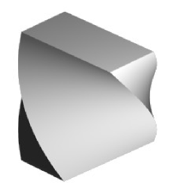
Figure 1: Example of a parity-breaking geometry. The object shown represents the cavity volume.

One way to ensure a breakdown of parity symmetry is to introduce a net chirality in the cavity geometry. We do this here by considering a helical cavity, as illustrated in Fig. 1. While we will assume that the cavity is empty, the technique described here is readily adapted to cases involving linear media.

The geometry of this cavity can be characterized using helical coordinates $x^{a}$, $a=1,2,3$, related to standard cartesian coordinates $x^{j}$, $j=x,y,z$, through $x^{1}=x^{x}\cos\alpha x^{z}-x^{y}\sin\alpha x^{z}$, $x^{2}=x^{x}\sin\alpha x^{z}+x^{y}\cos\alpha x^{z}$, $x^{3}=x^{z}$. Here we consider a cavities with perfectly conducting boundaries at $x^{a}=\pm X^{a}$, where $X^{a}$ are positive constants that specify the cross-sectional and length dimensions of the cavity. The parameter $\alpha$ determines the amount of rotation in the cavity about the $x^{3}$ central axis. For example, in Sec. IV.3 we take $X^{1}=1/2$, $X^{2}=1$, $X^{3}=1$, and $\alpha=45^{\circ}$. This gives a cavity with a rectangular cross section and a quarter left-handed turn from end to end, as in Fig. 1.

In curvilinear coordinates, the conventional Maxwell equations take the form

$$g^{-1/2}\ \epsilon^{abc}\partial_{b}E_{c}+\partial_{0}B^{a} =0\ , \quad\nabla_{a}B^{a}=0\ ,$$ (10)

$$g^{-1/2}\ \epsilon^{abc}\partial_{b}B_{c}-\partial_{0}E^{a} =0\ , \quad\nabla_{a}E^{a}=0\ ,$$ (11)

where $E^{a}$ and $B^{a}$ are contravariant field components, and $E_{a}=g_{ab}E^{b}$ and $B_{a}=g_{ab}B^{b}$ are covariant components. Here, $g_{ab}$ is the metric in curvilinear coordinates, and $\nabla_{a}$ is the associated covariant derivative. Note that the determinant $g=\det g_{ab}=1$ in the helical coordinates used here.

One advantage to using curvilinear coordinates is that the boundary conditions become relatively simple. Perfect-conductor boundary conditions imply that $E$ is perpendicular and $B$ parallel to the conducting surfaces of the cavity. As an example, consider a conducting boundary whose surface is represented by constant $x^{1}$. The contravariant basis vector $\mbox{\boldmath$e$}^{1}$ is perpendicular to this surface, and covariant vectors $\mbox{\boldmath$e$}_{2}$ and $\mbox{\boldmath$e$}_{3}$ are parallel to the surface. So, we must have $\mbox{\boldmath$E$}=E_{1}\mbox{\boldmath$e$}^{1}$ and $\mbox{\boldmath$B$}=B^{2}\mbox{\boldmath$e$}_{2}+B^{3}\mbox{\boldmath$e$}_{3}$ at this boundary. In our case, this implies $E_{1,2}$ vanish at the ends ($x^{3}=\pm X^{3}$), $E_{2,3}=0$ at $x^{1}=\pm X^{1}$, and $E_{3,1}=0$ at $x^{2}=\pm X^{2}$. For $B$, we get vanishing $B^{3}$ on the ends, $B^{1}=0$ at $x^{1}=\pm X^{1}$, and $B^{2}=0$ at $x^{2}=\pm X^{2}$.

IV.2 Discrete solutions

In order to show that the chiral geometry described above does in fact produce sensitivity to parity-odd Lorentz violations, we perform a numerical analysis of the its lowest-frequency resonances. Finite-difference-time-domain (FDTD) methods fdtd provide a straightforward procedure for estimating the $\cal M$ matrices over a range of frequencies. In this section, we develop a FDTD procedure for curvilinear coordinates.

We begin by defining discrete time by taking $t_{N}=\delta t\cdot N$, where $\delta t$ is a small time interval, and $N$ is an integer. The discrete fields are then taken as $\mbox{\boldmath$E$}_{N}=\mbox{\boldmath$E$}(t_{N})$ and $\mbox{\boldmath$B$}_{N}=\mbox{\boldmath$B$}(t_{N}-\delta t/2)$. This leads to discrete Maxwell equations:

$$(B^{a})_{N+1} \simeq(B^{a})_{N}-\delta t\ \epsilon^{abc}(\partial_{b}E_{c})_{N}\ ,$$ (12)

$$(E^{a})_{N+1} \simeq(E^{a})_{N}+\delta t\ \epsilon^{abc}(\partial_{b}B_{c})_{N+1}\ ,$$ (13)

where we have assumed $g=1$. This result allows us to “leapfrog” through time by iteratively applying Eq. (12) followed by (13).

For spatial dimensions, we construct a grid in helical coordinates,

$$(x^{1})_{J} = \ J\cdot\delta x^{1} -X^{1}\ ,$$

$$(x^{2})_{K} = \ K\cdot\delta x^{2} -X^{2}\ ,$$ (14)

$$(x^{3})_{L} = \ L\cdot\delta x^{3} -X^{3}\ ,$$

where $\delta x^{a}$ are small spatial intervals, $J,K,L$ are integers, and $-X^{a}$ represent the low edges of the cavity. We then construct a pair of lattices containing field values $(E_{a})_{NJKL}$ and $(B^{a})_{NJKL}$ defined at these spatial points.

In order to apply Eqs. (12) and (13), we need estimates for the spatial derivatives. Whenever possible, we use the symmetric forms

$$(\partial_{1}f)_{NJKL} \simeq[f_{N(J+1)KL}-f_{N(J-1)KL}]/(2\delta x^{1})\ ,$$

$$(\partial_{2}f)_{NJKL} \simeq[f_{NJ(K+1)L}-f_{NJ(K-1)L}]/(2\delta x^{2})\ ,$$ (15)

$$(\partial_{3}f)_{NJKL} \simeq[f_{NJK(L+1)}-f_{NJK(L-1)}]/(2\delta x^{3})\ .$$

These can be used at each of the interior nodes, but boundary nodes must be treated more carefully since derivatives (15) are not always defined at these points. Also, some care must be taken to ensure that the boundary conditions are satisfied at these nodes.

The method proceeds by stepping the $B$ field forward in time using Eqs. (12) and (15) for interior nodes. Next we propagate the boundary nodes. Here we illustrate the procedure for boundary nodes on the $J=0,\ x^{1}=-X^{1}$ surface. The generalization to other boundary surfaces is straightforward.

For $J=0$ boundary nodes, the boundary conditions imply vanishing $E_{2}$, $E_{3}$, and $B^{1}$. To propagate $B$ at one of these nodes using Eq. (12), we need the partial derivatives $\partial_{a}E_{b}$ for $a\neq b$. Since $E_{2,3}=0$ on this surface, the derivatives $\partial_{2}E_{3}$ and $\partial_{3}E_{2}$ vanish. This implies that $B^{1}$ remains zero provided that it vanished to begin with, as required by the boundary conditions. The derivatives $\partial_{2}E_{1}$ and $\partial_{3}E_{1}$ can be estimated using the symmetric form (15). In contrast, Eq. (15) fails for $\partial_{1}E_{2}$ and $\partial_{1}E_{3}$, since it would require field values at nodes outside of the cavity. So, in these cases we use the one-sided derivative,

$$(\partial_{1}E_{2,3})_{NJKL}\big{|}_{J=0}\simeq(E_{2,3})_{N(J+1)KL}/\delta x^{1}\big{|}_{J=0}\ ,$$ (16)

where we take advantage of the boundary conditions $E_{2,3}=0$ at $J=0$. We now have estimates for all six spatial derivatives $\partial_{a}E_{b},\ a\neq b$ at these nodes and can use Eq. (12) to propagate $B$ at this boundary. The other boundary surfaces are then propagated one step in time using similar methods.

Next, we propagate $E$ at interior points using Eqs. (13) and (15). Again, we will illustrate the procedure for boundary nodes by considering the $x^{1}=-X^{1},\ J=0$ surface. Since $E_{2}$ and $E_{3}$ vanish on this surface, we only need to calculate the change in $E_{1}$. However, since Eq. (13) propagates contravariant components, some care is needed in developing a procedure that updates $E_{1}$, but leaves $E_{2}$ and $E_{3}$ unaltered. We do this by noting that

$$(E^{1})_{(N+1)}-(E^{1})_{N}$$

$$\quad\quad\quad=g^{11}\left((E_{1})_{(N+1)}-(E_{1})_{N}\right)$$ (17)

$$\quad\quad\quad\simeq\delta t\ \left((\partial_{2}B_{3})_{N+1}-(\partial_{3}B_{2})_{N+1}\right)\ ,$$

where we have used the fact that $E_{2,3}=0$ to write $E^{1}=g^{1a}E_{a}=g^{11}E_{1}$. Using this result, we can step $E_{1}$ fields in time at $J=0$ nodes with the relation

$$(E_{1})_{(N+1)}-(E_{1})_{N}$$

$$\quad\quad\quad\simeq\delta t\ \left((\partial_{2}B_{3})_{N+1}-(\partial_{3}B_{2})_{N+1}\right)/g^{11}\ .$$ (18)

Here, Eq. (15) is used to estimate spatial derivatives without difficulty. Again, the other boundary surfaces are propagated using the generalization of this method.

By repeating the above procedure, we can propagate the $B$ and $E$ fields in time indefinitely. Note that at each time step, the $E$ ($B$) fields at a given node depend on the prior $E$ ($B$) fields at that node and the prior $B$ ($E$) fields at adjacent nodes. This implies that $E$ and $B$ need not be defined at every node, and we may adopt a lattice of fields in which $E$ and $B$ are only defined at alternate nodes. For example, in this work we take $E$ defined at nodes with $J+K+L=\mbox{even}$, and $B$ defined at nodes with $J+K+L=\mbox{odd}$, forming two interlaced $\mbox{\boldmath$E$}_{NJKL}$ and $\mbox{\boldmath$B$}_{NJKL}$ lattices. There is nothing preventing us from defining $E$ and $B$ at each node, but, in doing so, the calculation would essentially decouple into the propagation of two independent sets of fields like the ones used here, doubling the amount of information that is necessary.

A similar observation in the cartesian case led to a “Yee cell” in which different field components are defined at different spatial points fdtd . In our case, the mixing of components resulting from the raising and lowering of spatial indices by way of the metric makes the usual Yee method impractical.

To initialize the calculation, we must first seed the cavity with divergenceless fields satisfying the boundary conditions. A convenient set of initial fields is obtained by taking the expressions for the usual transverse-magnetic (TM) and transverse-electric (TE) $B$ fields associated with a rectangular cavity with $\alpha=0$ and making the substitutions $\{B^{x},B^{y},B^{z}\}\rightarrow\{B^{1},B^{2},B^{3}\}$ and $\{x^{x},x^{y},x^{z}\}\rightarrow\{x^{1},x^{2},x^{3}\}$. For simplicity, we simply set the initial $E$ fields to zero. The resulting initial fields obey the correct boundary conditions and can be shown to be divergenceless. Once the fields are set to these valid initial values, we can then propagate the fields in time using the above procedure.

IV.3 Results

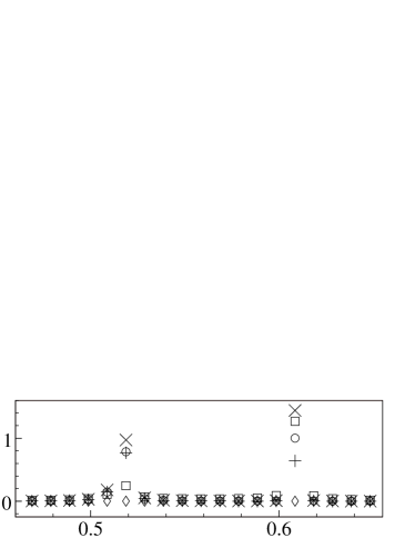
frequency

Figure 2: Numerically-determined lowest-frequency resonances for a cavity with $X^{1}=1/2$, $X^{2}=1$, $X^{3}=1$, and $\alpha=45^{\circ}$. Circles represent the energy $U$ versus frequency. Magnitudes of parity-odd $\cal\widetilde{M}$ matrices are plotted as $100\times U\times|{\cal\widetilde{M}}_{o+}|$ (diamonds) and $100\times U\times|{\cal\widetilde{M}}_{o-}|$ (squares). For comparison, we also show $5\times U\times|{\cal\widetilde{M}}_{e+}|$ ($\times$ signs) and $5\times U\times|{\cal\widetilde{M}}_{e-}|$ ($+$ signs). All values are normalized so that the maximum energy $U_{max}=1$ in arbitrary units.

We next apply the method described in the previous section to the cavity shown in Fig. 1. The dimensions of the cavity, in arbitrary spacetime units, are taken as $X^{1}=1/2$, $X^{2}=1$, and $X^{3}=1$. Taking $\alpha=45^{\circ}$ gives a quarter left-handed twist as shown in the figure. Applying the initialization method described above, we set initial-field values using the conventional expressions for the magnetic fields associated with the TM₁₁₀ mode for the analogous rectangular cavity with $\alpha=0$.

We use a spatial lattice 50 nodes wide in each of the three helical coordinates. We take a total time interval of 100 and calculate a total of 20,000 time steps. In order to reduce the amount of data saved to disk, we only record the field values for every fiftieth step. A fast fourier transform is performed on the saved field values, at each spatial node, yielding frequency-domain data. Using these, we determine the energy $U$ and the $\cal\widetilde{M}$ matrices, in cartesian coordinates, as a function of frequency. The results near the two lowest resonances are shown in Fig. 2. The matrix magnitudes, $|{\cal M}|=\sqrt{{\cal M}^{jk}{\cal M}^{jk}}$, for ${\cal\widetilde{M}}_{e+}$, ${\cal\widetilde{M}}_{e-}$, ${\cal\widetilde{M}}_{o+}$, and ${\cal\widetilde{M}}_{o-}$ are shown in the figure.

As expected, this parity-breaking configuration gives rise to a nonzero ${\cal\widetilde{M}}_{o-}$ at both of the resonances shown in Fig. 2, demonstrating sensitivity to the parity-odd violations associated with $\tilde{\kappa}_{o-}$. Furthermore, we find that ${\cal\widetilde{M}}_{o+}=0$ to within the errors of the calculation. This confirms the predictions of Sec. III, showing that while sensitivities to parity-odd Lorentz violations are possible, sensitivity to the nonbirefringent parity-odd violations cannot be achieved in resonators with simple isotropic magnetic media. We also note that $|{\cal\widetilde{M}}_{o-}|$ appears to be significantly smaller in the lower-frequency resonance, suggesting that sensitivities to parity-odd Lorentz violations are likely to be strongly dependent on the resonant mode excited in the cavity.

For both of the resonances in Fig. 2, we find nonzero ${\cal\widetilde{M}}_{e+}$ and ${\cal\widetilde{M}}_{e-}$ matrices, demonstrating sensitivity to the violations associated with $\tilde{\kappa}_{e+}$ and $\tilde{\kappa}_{e-}$, as in parity-even cavities. We note that the sensitivities to parity-odd violations in this example are larger by roughly a order of magnitude relative to parity-even violations. This geometric suppression shows that even in resonators with significant parity asymmetries, sensitivity to parity-odd violations may be small compared to those for parity-even violations. Nevertheless, this demonstrates the potential for at least a thousand-fold improvement in sensitivity to parity-odd Lorentz violations, assuming cavities of this type could be constructed and achieve stabilities comparable to their symmetric counterparts.

V summary and outlook

At present, resonant-cavity experiments have achieved sensitivities near $10^{-16}$ to parity-even coefficients for Lorentz violation cavities . The parity-odd coefficients enter through suppressed boost effects, resulting in constraints that are larger by approximately four orders of magnitude. Here we have shown that resonant cavities that do not respect parity symmetry can provide unsuppressed sensitivity to parity-odd Lorentz violations. Parity asymmetries can be introduced through the geometry of the cavity or by incorporating parity-breaking media.

In principle, the parity-odd coefficients $\tilde{\kappa}_{o+}$ and $\tilde{\kappa}_{o-}$ can cause observable violations of rotation symmetry in parity-breaking cavities, leading to improved sensitivities. In particular, this idea could be used to make significantly tighter constraints on the nonbirefringent $\tilde{\kappa}_{o+}$ coefficients. However, some thought must go into the design of a resonator to ensure sensitivity to $\tilde{\kappa}_{o+}$. In Sec. III, we have shown that a given resonator will be insensitive to certain combinations of coefficients. More specifically, we have shown that sensitivity to the three coefficients in $\tilde{\kappa}_{o+}$ is not possible in cavities incorporating only simple isotropic magnetic media.

Better sensitivities to $\tilde{\kappa}_{o+}$ could be achieved in resonators utilizing a combination of anisotropic magnetic media, with nondegenerate $\epsilon_{HB}$, in conjunction with asymmetric geometries or by using parity-violating media with nonzero $\epsilon_{DB}$. Chiral media chiral provide another interesting possibility. Assuming stabilities comparable to those in current experiments, parity-asymmetric resonators have the potential to improve the constraints on $\tilde{\kappa}_{o+}$ coefficients by four orders of magnitude by circumventing the boost suppression associated with Kennedy-Thorndike tests.

Resonators of this type could also be used to place improved laboratory-bounds on the five parity-odd coefficients in $\tilde{\kappa}_{o-}$. While cavity tests are not likely to achieve the same kind of sensitivities that are obtained in searches for birefringence, these experiments could provide a valuable laboratory-based check on astrophysical bounds. As illustrated in Sec. IV, sensitivities to $\tilde{\kappa}_{o-}$ can be improved simply by using parity-breaking geometries.

Finding geometries and media that maximize sensitivities to parity-odd effects remains an interesting open problem. The construction of high-Q asymmetric cavities may also pose a technological challenge. However, development of parity-breaking resonators would provide another avenue for high-precision tests of Lorentz invariance that would compliment the current parity-symmetric experiments. They have the potential to yield significant improvements in sensitivities to parity-odd Lorentz violation and could rival the best tests in any sector.

References

- (1) A.A. Michelson and E.W. Morley, Am. J. Sci. 34, 333 (1887); Phil. Mag. 24, 449 (1887).
- (2) R.J. Kennedy and E.M. Thorndike, Phys. Rev. 42, 400 (1932).
- (3) J. Lipa et al., Phys. Rev. Lett. 90, 060403 (2003); H. Müller et al., Phys. Rev. Lett. 91, 020401 (2003); H. Müller et al., Phys. Rev. D 67, 056006 (2003); Phys. Rev. D 68, 116006 (2003); P. Wolf et al., Gen. Rel. Grav. 36, 2352 (2004); P. Wolf et al., Phys. Rev. D 70, 051902 (2004); H. Müller, Phys. Rev. D 71, 045004 (2005); P.L. Stanwix et al., Phys. Rev. Lett. 95, 040404 (2005); Phys. Rev. D 74, 081101 (2006); S. Herrmann et al., Phys. Rev. Lett. 95, 150401 (2005); P. Antonini et al., Phys. Rev. A 71, 050101 (2005).
- (4) V.A. Kostelecký and S. Samuel, Phys. Rev. D 39, 683 (1989); 40, 1886 (1989); Phys. Rev. Lett. 63, 224 (1989); 66, 1811 (1991).
- (5) V.A. Kostelecký and R. Potting, Nucl. Phys. B 359, 545 (1991); Phys. Lett. B 381, 89 (1996); Phys. Rev. D 63, 046007 (2001); V.A. Kostelecký, M. Perry, and R. Potting, Phys. Rev. Lett. 84, 4541 (2000).
- (6) S.M. Carroll et al., Phys. Rev. Lett. 87, 141601 (2001); Z. Guralnik, R. Jackiw, S.Y. Pi, and A.P. Polychronakos, Phys. Lett. B 517, 450 (2001); C.E. Carlson, C.D. Carone, and R.F. Lebed, Phys. Lett. B 518, 201 (2001); A. Anisimov, T. Banks, M. Dine, and M. Graesser, Phys. Rev. D 65, 085032 (2002); I. Mocioiu, M. Pospelov, and R. Roiban, Phys. Rev. D 65, 107702 (2002); M. Chaichian, M.M. Sheikh-Jabbari, and A. Tureanu, hep-th/0212259; J.L. Hewett, F.J. Petriello, and T.G. Rizzo, Phys. Rev. D 66, 036001 (2002).
- (7) R. Gambini and J. Pullin, in V.A. Kostelecký, ed., CPT and Lorentz Symmetry, World Scientific, Singapore, 1999; J. Alfaro, H.A. Morales-Técotl, L.F. Urrutia, Phys. Rev. D66, 124006 (2002); D. Sudarsky, L. Urrutia, and H. Vucetich, Phys. Rev. Lett. 89, 231301 (2002); Phys. Rev. D 68, 024010 (2003); G. Amelino-Camelia, Mod. Phys. Lett. A 17, 899 (2002); Y.J. Ng, Mod. Phys. Lett. A18, 1073 (2003); R. Myers and M. Pospelov, Phys. Rev. Lett. 90, 211601 (2003); N.E. Mavromatos, hep-ph/0305215.
- (8) C.D. Froggatt and H.B. Nielsen, hep-ph/0211106.
- (9) J.D. Bjorken, Phys. Rev. D 67, 043508 (2003).
- (10) For an overview see, for example, R. Bluhm, Living Rev. Rel. 8, 5 (2005); V.A. Kostelecký, ed., CPT and Lorentz Symmetry, World Scientific, Singapore, 1999; CPT and Lorentz Symmetry II, World Scientific, Singapore, 2002; CPT and Lorentz Symmetry III, World Scientific, Singapore, 2005.
- (11) D. Colladay and V.A. Kostelecký, Phys. Rev. D 55, 6760 (1997); 58, 116002 (1998).
- (12) V.A. Kostelecký, Phys. Rev. D 69, 105009 (2004).
- (13) Q. Bailey and V.A. Kostelecký, Phys. Rev. D 70, 076006 (2004).
- (14) M.E. Tobar et al., Phys. Rev. D 71, 025004 (2005).
- (15) V.A. Kostelecký and M. Mewes, Phys. Rev. D 66, 056005 (2002).
- (16) V.A. Kostelecký and M. Mewes, Phys. Rev. Lett. 87, 251304 (2001); Phys. Rev. Lett. 97, 140401 (2006).
- (17) S.M. Carroll, G.B. Field, and R. Jackiw, Phys. Rev. D 41, 1231 (1990).
- (18) M.P. Haugan and F. Kauffmann, Phys. Rev. D 52, 3168 (1995); R. Jackiw and V.A. Kostelecký, Phys. Rev. Lett. 82, 3572 (1999); C. Adam and F.R. Klinkhamer, Nucl. Phys. B 657, 214 (2003); H. Müller, C. Braxmaier, S. Herrmann, A. Peters, and C. Lämmerzahl, Phys. Rev. D 67, 056006 (2003); T. Jacobson, S. Liberati, and D. Mattingly, Phys. Rev. D 67, 124011 (2003); V.A. Kostelecký, R. Lehnert, and M.J. Perry, Phys. Rev. D, 68, 123511 (2003); V.A. Kostelecký and A.G.M. Pickering, Phys. Rev. Lett. 91, 031801 (2003); R. Lehnert, Phys. Rev. D 68, 085003 (2003); G.M. Shore, Nucl. Phys. B 717, 86 (2005); B. Altschul and V.A. Kostelecký, Phys. Lett. B 628, 106 (2005); R. Bluhm and V.A. Kostelecký, Phys. Rev. D 71, 065008 (2005); B. Altschul, hep-th/0609030.
- (19) C.D. Carone, M. Sher, and M. Vanderhaeghen, Phys. Rev.D 74, 077901 (2006).
- (20) L.R. Hunter et al., in V.A. Kostelecký, ed., CPT and Lorentz Symmetry, World Scientific, Singapore, 1999; V.A. Kostelecký and C.D. Lane, Phys. Rev. D 60, 116010 (1999); J. Math. Phys. 40, 6245 (1999); D. Bear et al., Phys. Rev. Lett. 85, 5038 (2000); D.F. Phillips et al., Phys. Rev. D 63, 111101 (2001); M.A. Humphrey et al., physics/0103068; Phys. Rev. A 62, 063405 (2000); F. Cane et al., Phys. Rev. Lett. 93, 230801 (2004); P. Wolf et al., Phys. Rev. Lett. 96, 060801 (2006).
- (21) R. Bluhm et al., Phys. Rev. Lett. 88, 090801 (2002); Phys. Rev. D 68, 125008 (2003).
- (22) OPAL Collaboration, R. Ackerstaff et al., Z. Phys. C 76, 401 (1997); BELLE Collaboration, K. Abe et al., Phys. Rev. Lett. 86, 3228 (2001); KTeV Collaboration, H. Nguyen, in V.A. Kostelecký, ed., CPT and Lorentz Symmetry II, World Scientific, Singapore, 2002; FOCUS Collaboration, J.M. Link et al., Phys. Lett. B 556, 7 (2003); BaBar collaboration, B. Aubert et al., Phys. Rev. D 70, 012007 (2004); Phys. Rev. Lett. 92, 142002 (2004); hep-ex/0607103.
- (23) D. Colladay and V.A. Kostelecký, Phys. Lett. B 344, 259 (1995); Phys. Rev. D 52, 6224 (1995); Phys. Lett. B 511, 209 (2001); V.A. Kostelecký and R. Van Kooten, Phys. Rev. D 54, 5585 (1996); O. Bertolami et al., Phys. Lett. B 395, 178 (1997); V.A. Kostelecký, Phys. Rev. Lett. 80, 1818 (1998); Phys. Rev. D 61, 016002 (2000); 64, 076001 (2001); N. Isgur et al., Phys. Lett. B 515, 333 (2001); B. Altschul, hep-ph/0610324; hep-ph/0608094.
- (24) H. Dehmelt et al., Phys. Rev. Lett. 83, 4694 (1999); R. Mittleman et al., Phys. Rev. Lett. 83, 2116 (1999); G. Gabrielse et al., Phys. Rev. Lett. 82, 3198 (1999); R. Bluhm et al., Phys. Rev. Lett. 82, 2254 (1999); Phys. Rev. Lett. 79, 1432 (1997); Phys. Rev. D 57, 3932 (1998).
- (25) R. Bluhm and V.A. Kostelecký, Phys. Rev. Lett. 84, 1381 (2000); B. Heckel, in V.A. Kostelecký, ed., CPT and Lorentz Symmetry II, World Scientific, Singapore, 2002; L.-S. Hou, W.-T. Ni, and Y.-C.M. Li, Phys. Rev. Lett. 90, 201101 (2003); B. Altschul, Phys. Rev. D 72, 085003 (2005); Phys. Rev. Lett. 96, 201101 (2006); Phys. Rev. D 74, 083003 (2006).
- (26) V.W. Hughes et al., Phys. Rev. Lett. 87, 111804 (2001); R. Bluhm et al., Phys. Rev. Lett. 84, 1098 (2000).
- (27) V.A. Kostelecky and M. Mewes, Phys. Rev. D 69 016005 (2004); 70 031902 (2004); 70 076002 (2004); LSND Collaboration, L.B. Auerbach et al., Phys. Rev. D 72 076004 (2005); M.D. Messier (Super Kamiokande), in V.A. Kostelecký, ed., CPT and Lorentz Symmetry III, World Scientific, Singapore, 2005; B.J. Rebel and S.F. Mufson (MINOS), in V.A. Kostelecký, ed., CPT and Lorentz Symmetry III, World Scientific, Singapore, 2005; T. Katori, A. Kostelecky, and R. Tayloe, Phys. Rev. D 74 105009 (2006).
- (28) D.L. Anderson, M. Sher, I. Turan, Phys. Rev. D 70, 016001 (2004).
- (29) Q. Bailey and V.A. Kostelecký, Phys. Rev. D 74, 045001 (2006).
- (30) V.A. Kostelecký and R. Potting, Gen. Rel. Grav. 37, 1675 (2005).
- (31) V.A. Kostelecký and R. Potting, Phys. Rev. D 51, 3923 (1995).
- (32) V.A. Kostelecký and R. Lehnert, Phys. Rev. D 63, 065008 (2001).
- (33) J.A. Kong, Electromagnetic Wave Theory, Wiley, New York, 1990.
- (34) J.D. Jackson, Classical Electrodynamics, 3rd ed., Wiley, New York, 1999.
- (35) K. Yee, IEEE Trans. Ant. Prop. 14, 302 (1966).
- (36) See, for example, John Lekner, Pure Appl. Opt. 5, 417 (1996).