Abstract

We present an extension of the minimal split supersymmetry model, which is capable of explaining the baryon asymmetry of the Universe. Instead of MSSM we start from NMSSM and split its spectrum in such a way that the low energy theory contains neutral particles, in addition to the content of minimal split supersymmetry. They trigger the strongly first order electroweak phase transition (EWPT) and provide an additional source of CP-violation. In this model, we estimate the amount of the baryon asymmetry produced during EWPT, using WKB approximation for CP-violating sources in diffusion equations. We also examine the contribution of CP-violating interactions to the electron and neutron electric dipole moments and estimate the production of the neutralino dark matter. We find that both phenomenological and cosmological requirements can be fulfilled in this model.

PACS numbers: 11.30.Fs, 13.40.Em, 14.80.Ly, 95.35.+d,

1 Introduction

In spite of approximate symmetry between particles and antiparticles, our visible Universe is asymmetric in baryons. An explanation of this fact ought to be addressed in any viable theory. Quantitatively, the measurements of the anisotropy of the cosmic microwave background constrain the baryon-to-photon ratio [1] to be in the range

$$6.1\times 10^{-10}<\frac{n_{B}}{n_{\gamma}}<6.9\times 10^{-10}.$$ (1)

Three necessary conditions (Sakharov conditions) must be fulfilled in the early Universe to produce the baryon asymmetry [2]: baryon number violation, C- and CP-violation and departure from thermal equilibrium.

Electroweak baryogenesis [3] is one of the most interesting scenarios of baryon asymmetry generation. If the electroweak phase transition (EWPT) is of the first order, it provides departure from thermal equilibrium in cosmic plasma, as it proceeds through nucleation of bubbles of the broken phase, their subsequent growth and percolation. The baryon asymmetry generated during the phase transition can be washed out by rapid sphaleron processes in the broken phase [4]. In the Standard Model, the condition

$$\frac{v_{c}}{T_{c}}\mathchoice{\mathrel{\vbox{\hbox{$\buildrel\displaystyle>\over{\displaystyle\sim}$}}}}{\mathrel{\vbox{\hbox{$\buildrel\textstyle>\over{\textstyle\sim}$}}}}{\mathrel{\vbox{\hbox{$\buildrel\scriptstyle>\over{\scriptstyle\sim}$}}}}{\mathrel{\vbox{\hbox{$\buildrel\scriptscriptstyle>\over{\scriptscriptstyle\sim}$}}}}1.1$$ (2)

(where $T_{c}$ is the critical temperature and $v_{c}$ is the Higgs expectation value at this temperature) would ensure that the sphaleron transitions are suppressed inside the bubbles of the new phase [5] and the baryon asymmetry survives. Nonperturbative analysis [6] revealed that, with the present experimental bound on the Higgs boson mass, the electroweak phase transition in the Standard Model not only does not yield (2), but is definitely not of the first order. Moreover, in spite of the presence of CP-violating phase in CKM matrix, its contribution to the production of the baryon asymmetry is too small to explain the observed value (1). The Standard Model fails to support electroweak baryogenesis.

Supersymmetry is one of the most attractive ways beyond the framework of the Standard Model. One recalls the cancellation of quadratic divergences and gauge coupling unification among the main reasons for interest in supersymmetric theories. Minimal Supersymmetric Standard Model (MSSM) and its extensions suggest the lightest supersymmetric particle (LSP) as a natural dark matter candidate and provide mechanisms to generate the baryon asymmetry (for recent studies see Refs. [7], [8], [9], [10] and references therein).

Recently, motivated by landscape of vacua in string theory and cosmological constant problem, models with split supersymmetry have been proposed [11, 12]. The spectrum of these models is governed by two scales. While the electroweak scale $m_{ew}$ determines the masses of the Standard Model particles and additional fermionic degrees of freedom (higgsinos and gauginos) the other MSSM particles (scalars) have masses of order of a splitting scale $m_{s}$, which generally may be in a wide range of $10^{4}-10^{15}$ GeV. Such a pattern ensures the gauge coupling unification, so that split SUSY can be incorporated into a GUT.

Split SUSY enables one to avoid phenomenological difficulties with CP- and flavor violation and also provides natural dark matter candidates. But from the point of view of the electroweak baryogenesis, split supersymmetry, in its minimal version, shares some disadvantages of SM: the electroweak phase transition remains too weak, because the additional, weakly coupled fermions do not strengthen EWPT. It is of interest to find a viable scenario, which would be compatible with general split supersymmetry framework and would provide conditions required for effective electroweak baryogenesis. One way, proposed in Ref. [14], is to spoil the supersymmetric relations between the gauge and Yukawa gaugino-higgsino couplings. For rather large Yukawas, the charginos and neutralinos are light in the symmetric phase but heavy in the broken phase, so they decouple from the cosmic plasma at the moment of the phase transition. During the EWPT the particle species to be decoupled transfer their entropy to the cosmic plasma, that results in the increase of the temperature and the delay of the transition, providing a possibility to satisfy the inequality (2).

In this paper we pursue another approach and propose a model which keeps all phenomenologically interesting properties of the minimal split supersymmetry and at the same time is capable of producing the baryon asymmetry at EWPT. Instead of using MSSM as a starting point, we begin with Non-Minimal Supersymmetric Standard Model (NMSSM) and split its spectrum in such a way as to provide the low energy theory with all features required for successful electroweak baryogenesis. Indeed, additional neutral scalar fields, which are left at low energies after the spectrum splitting, change zero temperature potential and can make EWPT stronger. The model contains new sources of CP-violation as well. Apart from their crucial role in the generation of the required amount of the baryon asymmetry (1), they also contribute to the electric dipole moments (EDMs) of electron and neutron at the level detectable in the near future experiments. Also, we study the possibility that the lightest neutralino is dark matter particle. We find that along with gaugino- and higgsino-like candidates there is a region of parameter space where dark matter is mostly singlino.

The outline of this paper is as follows. Sec. 2 contains the description of our model and its main features. In Sec. 3 we study the strength of the electroweak phase transition and show that EWPT can be the strongly first order. In Sec. 4 we describe the baryon asymmetry calculation procedure and present numerical results. In Sec. 5 we estimate the values of electron and neutron EDMs in our model. Neutralino dark matter phenomenology is discussed in Sec. 6 and Sec. 7 contains our conclusions.

2 The model

We begin with the most general NMSSM. The relevant for our study part of the superpotential is [15]

$$W=\lambda\hat{N}\hat{H}_{u}\epsilon\hat{H}_{d}+\frac{1}{3}k\hat{N}^{3}+\mu\hat{H}_{u}\epsilon\hat{H}_{d}+r\hat{N}.$$ (3)

Here $\hat{H}_{u}$ and $\hat{H}_{d}$ are the Higgs doublets, $\hat{N}$ is a chiral superfield, which is a singlet with respect to the SM gauge group and $\epsilon$ is antisymmetric $2\times 2$ matrix, $\epsilon_{12}=1$. Soft SUSY breaking terms for this model read

$$V_{soft}=\left(\lambda A_{\lambda}NH_{u}\epsilon H_{d}+\frac{1}{3}kA_{k}N^{3}+\mu BH_{u}\epsilon H_{d}+A_{r}N+h.c.\right)$$ (4)

$$+m_{u}^{2}H_{u}^{\dagger}H_{u}+m_{d}^{2}H_{d}^{\dagger}H_{d}+m_{N}^{2}|N|^{2}.$$

Electroweak baryogenesis in NMSSM has been explored in Refs. [8] in the context of low energy supersymmetry breaking. We consider this model in the framework of split SUSY. For this purpose some parameters need to be fine-tuned, like in the minimal split SUSY, in such a way that the particle spectrum is split into two parts. To strengthen the electroweak phase transition, some scalars can be recruited [16]. To preserve gauge coupling unification, these particles should not contribute to the beta functions (or their contributions should be canceled) at least at the leading order. So in the minimal case, the low energy theory can contain (besides the usual split SUSY particles) singlets with respect to the SM gauge group.

We consider the theory in which the only new source of explicit CP-violation is $\mu$-parameter which for concreteness we take to be exactly imaginary. All other parameters (including $B\mu$-term) of the theory (3), (4) are taken to be real (except in the analysis of the electron and neutron EDMs). This is a purely technical assumption which we make in order that the parameter space to be tractable.

We examine splitting in the $(H_{u},H_{d},N)$ sector only, because decoupling of squarks and sleptons is supposed to be similar to the case of the minimal split SUSY. The tree level scalar potential of NMSSM is

$$V=V_{D}+V_{F}+V_{soft}\;,$$ (5)

where

$$V_{D}=\frac{g^{2}}{8}\left(H^{\dagger}_{d}\sigma_{a}H_{d}+H^{\dagger}_{u}\sigma_{a}H_{u}\right)^{2}+\frac{g^{\prime 2}}{8}\left(|H_{d}|^{2}-|H_{u}|^{2}\right)^{2},$$ (6)

$$V_{F}=|\lambda H_{u}\epsilon H_{d}+kN^{2}+r|^{2}+|\lambda N+\mu|^{2}\left(H_{u}^{\dagger}H_{u}+H_{d}^{\dagger}H_{d}\right),$$ (7)

and the Higgs doublets are $H_{u}=\left(H_{u}^{+},H_{u}^{0}\right)^{T}$ and $H_{d}=\left(H_{d}^{0},H_{d}^{-}\right)^{T}$. Let us choose the vacuum expectation values for neutral scalars as follows,

$$\langle H_{d}^{0}\rangle=\frac{1}{\sqrt{2}}v_{d},\;\;\;\langle H_{u}^{0}\rangle=\frac{1}{\sqrt{2}}v_{u}e^{i\phi_{H}},\;\;\;\langle N\rangle=\frac{1}{\sqrt{2}}\left(v_{S}+iv_{P}\right)\equiv\frac{1}{\sqrt{2}}\sqrt{v_{S}^{2}+v_{P}^{2}}e^{i\phi_{S}}.$$

Here we have taken into account that the effective potential depends only on the sum of the phases of vev’s of the Higgs doublets and one of these phases can be set equal to zero by a gauge transformation. The stationarity condition with respect to the phase $\phi_{H}$, $\partial V/\partial\phi_{H}=0$, gives the following relation

$$\sin{\phi_{H}}=-\frac{\frac{k\lambda}{2}\left(v_{S}^{2}+v_{P}^{2}\right)\sin{(\phi_{H}-2\phi_{S})}+\frac{\lambda A_{\lambda}}{\sqrt{2}}\sqrt{v_{S}^{2}+v_{P}^{2}}\sin{(\phi_{S}+\phi_{H})}}{B\mu+\lambda r}.$$ (8)

To split the spectrum of the theory, we take soft SUSY breaking parameters $B\mu$, $m_{u}^{2}$ and $m_{d}^{2}$ of the order of the splitting scale $m_{s}^{2}$ and all other parameters in the scalar sector (including all vev’s) of the order of the electroweak scale $m_{ew}$. Equation (8) implies the estimate $|\phi_{H}|\sim\left(m_{ew}/m_{s}\right)^{2}$ and therefore this phase can be safely neglected in the following analysis.

We find that vev’s of the scalar fields at the minimum of the potential (5) must satisfy the following conditions

$$m_{u}^{2} = \frac{\bar{g}^{2}}{8}v^{2}\cos{2\beta}-\frac{\lambda^{2}}{2}v^{2}\cos^{2}{\beta}-\frac{\lambda^{2}}{2}v_{S}^{2}-\left(|\mu|+\frac{\lambda}{\sqrt{2}}v_{P}\right)^{2}+m_{A}^{2}\cos^{2}{\beta},$$ (9)

$$m_{d}^{2} = -\frac{\bar{g}^{2}}{8}v^{2}\cos{2\beta}-\frac{\lambda^{2}}{2}v^{2}\sin^{2}{\beta}-\frac{\lambda^{2}}{2}v_{S}^{2}-\left(|\mu|+\frac{\lambda}{\sqrt{2}}v_{P}\right)^{2}+m_{A}^{2}\sin^{2}{\beta},$$ (10)

$$m_{N}^{2}+2kr = \frac{1}{2}k\lambda v^{2}\sin{2\beta}-k^{2}\left(v_{S}^{2}+v_{P}^{2}\right)-\frac{\lambda^{2}}{2}v^{2}+\frac{\lambda A_{\lambda}}{2\sqrt{2}}\cdot\frac{v^{2}}{v_{S}}\sin{2\beta}$$

$$-\frac{kA_{k}}{\sqrt{2}}\left(v_{S}-\frac{v_{P}^{2}}{v_{S}}\right)-\sqrt{2}\frac{A_{r}}{v_{S}},$$

$$m_{N}^{2}-2kr = -\frac{1}{2}k\lambda v^{2}\sin{2\beta}-k^{2}\left(v_{S}^{2}+v_{P}^{2}\right)-\frac{\lambda^{2}}{2}v^{2}-\frac{\lambda|\mu|v^{2}}{\sqrt{2}v_{P}}+\sqrt{2}kA_{k}v_{S}v_{P},$$ (12)

where we use the notations $\tan{\beta}=v_{u}/v_{d}$, $v^{2}=v_{u}^{2}+v_{d}^{2}$, $\bar{g}^{2}=g^{2}+g^{\prime 2}$ and

$$m_{A}^{2}=\frac{2}{\sin{2\beta}}\left(\lambda r+\frac{k\lambda}{2}\left(v_{S}^{2}-v_{P}^{2}\right)+\frac{1}{\sqrt{2}}\lambda A_{\lambda}v_{S}+\mu B\right).$$

We expand the scalar fields about their vev’s as follows,

$${\rm Re}H_{d}^{0}=\frac{1}{\sqrt{2}}\left(v_{d}+h^{0}\cos{\beta}-H^{0}\sin{\beta}\right),\;\;{\rm Im}H_{d}^{0}=\frac{1}{\sqrt{2}}\left(A^{0}\sin{\beta}+G^{0}\cos{\beta}\right),$$

$${\rm Re}H_{u}^{0}=\frac{1}{\sqrt{2}}\left(v_{u}+h^{0}\sin{\beta}+H^{0}\cos{\beta}\right),\;\;{\rm Im}H_{u}^{0}=\frac{1}{\sqrt{2}}\left(A^{0}\cos{\beta}-G^{0}\sin{\beta}\right),$$

$$H_{d}^{-}=G^{-}\cos{\beta}+H^{-}\sin{\beta},\;\;H_{u}^{+}=H^{+}\cos{\beta}-G^{+}\sin{\beta},$$

$$N=\frac{1}{\sqrt{2}}\left(v_{S}+S+i(v_{P}+P)\right).$$

Here $G^{\pm}$ and $G^{0}$ are Goldstone modes which are eaten, due to the Higgs mechanism, by $W^{\pm}$- and $Z^{0}$-bosons, respectively, $h^{0}$ and $H^{0}$ are the neutral scalar Higgs bosons, $A^{0}$ is the Higgs pseudoscalar, $S$ and $P$ are singlet scalar and pseudoscalar fields.

Let us choose the basis in the space of neutral scalars as $(h^{0},H^{0},A^{0},S,P)$. By making use of the conditions (9) - (12), the elements of $5\times 5$ squared mass matrix for neutral scalars read as follows,

$$M_{11}^{2} = \frac{\bar{g}^{2}v^{2}}{4}\cos^{2}{2\beta}+\frac{\lambda^{2}v^{2}}{2}\sin^{2}{2\beta},$$ (13)

$$M_{22}^{2} = m_{A}^{2}-\frac{\lambda^{2}v^{2}}{2}\sin^{2}{2\beta}+\frac{\bar{g}^{2}v^{2}}{4}\sin^{2}{2\beta},$$ (14)

$$M_{33}^{2} = m_{A}^{2},$$ (15)

$$M_{44}^{2} = 2k^{2}v_{S}^{2}+\frac{\lambda A_{\lambda}}{2\sqrt{2}}\frac{v^{2}}{v_{S}}\sin{2\beta}+\frac{kA_{k}}{\sqrt{2}}\left(v_{S}+\frac{v_{P}^{2}}{v_{S}}\right)-\sqrt{2}\frac{A_{r}}{v_{S}},$$ (16)

$$M_{55}^{2} = 2k^{2}v_{P}^{2}-\frac{\lambda}{\sqrt{2}}\frac{|\mu|v^{2}}{v_{P}},$$ (17)

$$M_{12}^{2} = M_{21}^{2}=\left(\frac{\lambda^{2}}{4}-\frac{\bar{g}^{2}}{8}\right)v^{2}\sin{4\beta},$$ (18)

$$M_{13}^{2} = M_{31}^{2}=-k\lambda v_{S}v_{P}+\frac{\lambda A_{\lambda}}{\sqrt{2}}v_{P},$$ (19)

$$M_{14}^{2} = M_{41}^{2}=-k\lambda v_{S}v\sin{2\beta}+\lambda^{2}v_{S}v-\frac{\lambda A_{\lambda}}{\sqrt{2}}v\sin{2\beta},$$ (20)

$$M_{15}^{2} = M_{51}^{2}=k\lambda v_{P}v\sin{2\beta}+\sqrt{2}\lambda v\left(|\mu|+\frac{\lambda}{\sqrt{2}}v_{P}\right),$$ (21)

$$M_{23}^{2} = M_{32}^{2}=0,$$ (22)

$$M_{24}^{2} = M_{42}^{2}=-k\lambda v_{S}v\cos{2\beta}-\frac{\lambda A_{\lambda}}{\sqrt{2}}v\cos{2\beta},$$ (23)

$$M_{25}^{2} = M_{52}^{2}=k\lambda v_{P}v\cos{2\beta},$$ (24)

$$M_{34}^{2} = M_{43}^{2}=-k\lambda vv_{P},$$ (25)

$$M_{35}^{2} = M_{53}^{2}=-k\lambda vv_{S}+\frac{\lambda A_{\lambda}}{\sqrt{2}}v,$$ (26)

$$M_{45}^{2} = M_{54}^{2}=2k^{2}v_{S}v_{P}-\sqrt{2}kA_{k}v_{P}.$$ (27)

For the squared masses of the charged Higgs bosons one has $m_{H^{\pm}}^{2}=m_{A}^{2}-\frac{\lambda^{2}v^{2}}{2}+\frac{g^{2}v^{2}}{4}$. From the expressions for the scalar mass matrices it can be easily seen that, like in the minimal split SUSY, one can split the particle spectrum by taking $\mu B$ parameter of order of the squared splitting scale $m_{s}^{2}$. This means that the charged higgses, one scalar $H^{0}$ and one pseudoscalar $A^{0}$ from the Higgs sector become heavy. It is straightforward to check that the low energy effective Lagrangian is obtained by the same substitution for the Higgs doublets as in the minimal split SUSY [12]

$$H_{u}\to H\sin{\beta},\;\;\;H_{d}\to\epsilon H^{*}\cos{\beta},$$ (28)

where $H$ is the Standard Model Higgs doublet. After the replacement (28) and including interactions with fermions, we arrive at the Lagrangian for light degrees of freedom

$$\cal{L}=\cal{L}_{\rm{V}}+\cal{L}_{\rm{Y}}.$$

It consists of two parts: the scalar potential

$$-{\cal L_{\rm{V}}}=\frac{\bar{g}^{2}}{8}\cos^{2}{2\beta}\left(H^{\dagger}H\right)^{2}+|r+kN^{2}-\frac{\lambda}{2}\sin{2\beta}H^{\dagger}H|^{2}+|\lambda N+\mu|^{2}H^{\dagger}H$$

$$+\left(-\frac{\lambda}{2}A_{\lambda}\sin{2\beta}NH^{\dagger}H-\frac{\mu B}{2}\sin{2\beta}H^{\dagger}H+\frac{1}{3}kA_{k}N^{3}+A_{r}N+h.c.\right)$$ (29)

$$+\left(m_{u}^{2}\sin^{2}{\beta}+m_{d}^{2}\cos^{2}{\beta}\right)H^{\dagger}H+m_{N}^{2}|N|^{2}$$

and the Yukawa interactions

$$-{\cal L_{\rm{Y}}}=-\lambda N\tilde{H}_{u}\epsilon\tilde{H}_{d}-\lambda\sin{\beta}H^{T}\epsilon\left(\tilde{H}_{d}\tilde{n}\right)+\lambda\cos{\beta}\left(\tilde{n}\tilde{H}_{u}\right)H^{*}-kN\tilde{n}\tilde{n}+h.c.,$$ (30)

where $\tilde{H}^{u}$ and $\tilde{H}^{d}$ are higgsinos and $\tilde{n}$ is singlino, which is the fermionic component of the singlet chiral superfield $\hat{N}$. In the above expressions we omitted terms with the Yukawa couplings of quarks to the Higgs bosons, gaugino interactions and mass terms, which are the same as the ones in Ref. [12]. For this Lagrangian to describe the low energy physics, all terms are to be of the order of electroweak scale. Inspecting the Higgs mass term in (29) (see also eq. (33) below) and eqs. (9), (10), one can find that a strong cancellation in the combination $m_{u}^{2}\tan{\beta}+m_{d}^{2}\cot{\beta}-2B\mu$ has to take place.

A special feature of our model, as compared to the minimal split SUSY, is that after splitting there remain relatively light singlet fields: complex scalar $N$ and Majorana fermion $\tilde{n}$.

It is often assumed that NMSSM possesses ${\mathbb{Z}}_{3}$-symmetry, which implies $\mu=r=A_{r}=B\mu=0$. It was argued in Ref. [17], that the splitting of ${\mathbb{Z}}_{3}$-symmetric theory, which leads to the same particle content as the one described above, results in the relations $\lambda\sim\left(m_{ew}/m_{s}\right)^{2}$ and $\langle N\rangle\sim m_{s}^{2}/m_{ew}$; therefore, the cubic term in the scalar effective potential behaves effectively like quadratic during the electroweak phase transition. This means that EWPT cannot be strong enough in that case and electroweak baryogenesis does not work. Thus we do not impose the ${\mathbb{Z}}_{3}$-symmetry and take all parameters in (3) and (4) to be non-zero.

The Lagrangian (29), (30) describes interactions at the splitting scale $m_{s}$, which is taken below to be $10^{9}$ GeV, if not stated otherwise. To obtain the low energy theory, the couplings in (29), (30) should be changed according to the renormalization group equations (RGE). The set of RGE for dimensionless couplings is presented in Appendix A.

Below the splitting scale $m_{s}$, the theory is described by the following Lagrangian

$$-{\cal L_{\rm{V}}}=-m^{2}H^{\dagger}H+\frac{\tilde{\lambda}}{2}\left(H^{\dagger}H\right)^{2}+i\tilde{A}_{1}H^{\dagger}H\left(N-N^{*}\right)+\tilde{A}_{2}H^{\dagger}H\left(N+N^{*}\right)+\kappa_{1}|N|^{2}H^{\dagger}H$$

$$-\kappa_{2}H^{\dagger}H\left(N^{2}+N^{*2}\right)+\tilde{m}_{N}^{2}|N|^{2}+\lambda_{N}|N^{2}|^{2}+\frac{1}{3}\tilde{A}_{k}\left(N^{3}+N^{*3}\right)+\tilde{A}_{r}\left(N+N^{*}\right)$$ (31)

$$+\left(\frac{\tilde{m}^{2}}{2}N^{2}+\frac{1}{2}\tilde{A}_{3}N^{2}N^{*}+\xi N^{4}+\frac{\eta}{6}N^{3}N^{*}+h.c.\right)$$

and

$$-{\cal L_{\rm{Y}}}=\frac{M_{2}}{2}\tilde{W}^{a}\tilde{W}^{a}+\frac{M_{1}}{2}\tilde{B}\tilde{B}+\left(\mu+\kappa N\right)\tilde{H}^{T}_{u}\epsilon\tilde{H}_{d}-kN\tilde{n}\tilde{n}$$

$$+H^{\dagger}\left(\frac{1}{\sqrt{2}}\tilde{g}_{u}\sigma^{a}\tilde{W}^{a}+\frac{1}{\sqrt{2}}\tilde{g}_{u}^{\prime}\tilde{B}-\lambda_{u}\tilde{n}\right)\tilde{H}_{u}$$ (32)

$$+H^{T}\epsilon\left(-\frac{1}{\sqrt{2}}\tilde{g}_{d}\sigma^{a}\tilde{W}^{a}+\frac{1}{\sqrt{2}}\tilde{g}^{\prime}_{d}\tilde{B}-\lambda_{d}\tilde{n}\right)\tilde{H}_{d}+h.c.,$$

where we have also written explicitly the interactions between the Higgs bosons, higgsinos and gauginos. The terms, analogous to ones with couplings $\tilde{A}_{3},\xi,\eta$ in the last line in eq. (31), are absent in eq. (29), but they are generated below $m_{s}$ by quantum corrections coming from one-loop diagrams of the types presented in Fig. 1.

Figure 1: Examples of the Feynman diagrams, which generate terms in the last line in eq. (31).

Comparing the Lagrangians (29), (31) and (30), (32), we read off the following matching conditions between the coupling constants, which are valid at the splitting scale $m_{s}$,

$$m^{2}=-\left(m_{u}^{2}\sin^{2}{\beta}+m_{d}^{2}\cos^{2}{\beta}-\mu B\sin{2\beta}+|\mu|^{2}-\lambda r\sin{2\beta}\right),$$ (33)

$$\tilde{A}_{1}=\lambda\mu,\;\;\;\;\tilde{A}_{2}=-\lambda A_{\lambda}\sin{\beta}\cos{\beta},$$

$$\kappa_{1}=\lambda^{2},\;\;\;\;\kappa_{2}=-\lambda k\sin{\beta}\cos{\beta},\;\;\;\;\lambda_{N}=k^{2},$$

$$\tilde{A}_{k}=kA_{k},\;\;\;\tilde{m}^{2}=2kr,\;\;\;\tilde{A}_{r}=A_{r},\;\;\;\tilde{m}_{N}^{2}=m_{N}^{2},$$ (34)

$$\tilde{\lambda}=\frac{\bar{g}^{2}}{4}\cos^{2}{2\beta}+\frac{\lambda^{2}}{2}\sin^{2}{2\beta},\;\;\;\kappa=\lambda,$$ (35)

$$\lambda_{u}=\lambda\cos{\beta},\;\;\;\;\lambda_{d}=-\lambda\sin{\beta},$$ (36)

$$\tilde{A}_{3}=\eta=\xi=0$$ (37)

and, like in the minimal split SUSY,

$$\tilde{g}_{u}=g\sin{\beta},\;\;\;\tilde{g}_{d}=g\cos{\beta},\;\;\;\tilde{g}_{u}^{\prime}=g^{\prime}\sin{\beta},\;\;\;\tilde{g}_{d}^{\prime}=g^{\prime}\cos{\beta}.$$ (38)

The aforementioned cancellation in (33) results in $m^{2}\sim m_{ew}^{2}$. The matching conditions provide the initial values for RGE. We use 2-loop RGE for gauge couplings and 1-loop RGE for other dimensionless couplings, neglecting threshold effects. The coupling constants, additional to the minimal split SUSY, begin to contribute to the running of the gauge couplings only at 2-loop level and do not spoil their unification.

In the next section we investigate EWPT in this model and study the properties of one-loop effective potential. Its zero temperature part [21] is written in $\overline{\rm DR}$ scheme as follows,

$$V^{(1)}=\sum_{i}(\pm)\frac{1}{64\pi^{2}}n_{i}m_{i}^{4}\left[\log{\frac{m_{i}^{2}}{q^{2}}}-\frac{3}{2}\right],$$ (39)

where the sum runs over all particle species of field-dependent mass $m_{i}$ with $n_{i}$ degrees of freedom. Upper and lower signs correspond to the boson and fermion cases, respectively. The renormalization scale $q$ is chosen to be $100$ GeV. We include loop contributions from top quark, gauge and Higgs boson, singlet (pseudo)scalars. Let us single out the terms in $V_{tree}\equiv-{\mathcal{L}}_{V}$, which are quadratic in vev’s $v,\;v_{S}$ and $v_{P}$, e.g.,

$$V_{tree}=-\frac{m^{2}}{2}v^{2}+\frac{m_{S}^{2}}{2}\left(v_{S}^{2}+v_{P}^{2}\right)+\frac{\tilde{m}^{2}}{2}\left(v_{S}^{2}-v_{P}^{2}\right)+V_{tree}^{>2},$$ (40)

where the last term denotes the rest of the tree level potential. Imposing the conditions

$$-m^{2}+\frac{1}{v}\frac{\partial}{\partial v}\left(V_{tree}^{>2}+V^{(1)}\right)=0\;,$$ (41)

$$m_{S}^{2}+\tilde{m}^{2}+\frac{1}{v_{S}}\frac{\partial}{\partial v_{S}}\left(V_{tree}^{>2}+V^{(1)}\right)=m_{S}^{2}-\tilde{m}^{2}+\frac{1}{v_{P}}\frac{\partial}{\partial v_{P}}\left(V_{tree}^{>2}+V^{(1)}\right)=0\;,$$ (42)

one ensures that minimum remains at $(v,v_{S},v_{P})$.

Let us describe the part of the parameter space, relevant for our study. There are three dimensionless parameters $\tan{\beta},\;\lambda,\;k$, which a priori take any values compatible with the weak coupling regime in both high-energy and low-energy theories. In addition, the low-energy spectrum has to be phenomenologically viable. To reduce the parameter space of the model, in what follows we fix these dimensionless parameters at the splitting scale as (unless stated otherwise),

$$\tan{\beta}=10,\;\;\;\lambda=0.6,\;\;\;k=-0.5.$$ (43)

There is nothing special in this set, except of the choice of rather large value of $\tan{\beta}$. As it will be argued in Sec. 4, if $\tan{\beta}\sim 1$, produced amount of the baryon asymmetry is zero within the semiclassical approximation for CP-violating sources. Quantitatively, the numbers we obtain (the exact amount of the baryon asymmetry, predictions for EDMs, etc.) are stable with respect to small variations of these parameters about the point (43).

The dimensionful parameters are taken at the electroweak scale. So, we do not assume universal boundary conditions for soft supersymmetry breaking terms. Below we vary some of the parameters keeping several relations between them to simplify the analysis. For $m^{2},\;\tilde{m}_{N}^{2}$ and $\tilde{m}^{2}$ we substitute the corresponding expressions in terms of $v,\;v_{S}$ and $v_{P}$, which follow from eqs. (41), (42). Since we take $\mu$ to be imaginary and CP is violated in the Higgs sector, two scalars and one pseudoscalar generally mix. We restrict our considerations (the only reason is to reduce the number of free parameters) to the case where mixing between the physical Higgs boson and two other (pseudo)scalars is absent; in fact this can be achieved by tuning trilinear constants $\tilde{A}_{1},\;\tilde{A}_{2}$. Nonzero $\tilde{A}_{3}$ is generated by radiative corrections, hence generically it is small and is not very important, so we set it equal to zero. We also choose $\tilde{A}_{r}=0$ for concreteness. The free dimensionful parameters we are left with are vev’s of singlet scalars $v_{S},\;v_{P}$, gaugino masses $M_{1},\;M_{2},\;M_{3}$ and trilinear coupling constant $\tilde{A}_{k}$.

We use the RGE as follows. We take known values of the gauge and top Yukawa couplings derived from the following relations : $\alpha_{s}(M_{Z})=0.117$, $y_{t}(m_{t})=0.95$, $M_{Z}=91.19$ GeV, $M_{W}=80.42$ GeV. These four couplings run up to the scale $\mu=m_{s}$ according to truncated RGE, in which we leave only $y_{t}$, $g_{i}$, $i=1,2,3$. At the splitting scale we take the set of other parameters in (31) and (32), obeying initial conditions (43) and matching conditions (35-38). Then all couplings run down to the electroweak scale in accordance with the full set of RGE. Because of additional coupling constants in RGE, the procedure described above does not give the correct low energy pattern of gauge and top Yukawa couplings we started with. Therefore, we tune top Yukawa coupling at the splitting scale $m_{s}$ and check that obtained values of $g_{1},g_{2},g_{3}$ and $y_{t}$ at the electroweak scale are within experimental error bars. Also we check that all couplings remain in the perturbative regime up to the GUT scale.

In our restricted parameter space we use RGE to obtain the Higgs boson mass $m_{h}$. The dependence of $m_{h}$ on the splitting scale $m_{s}$ is plotted in Fig. 2.

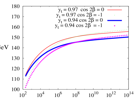
Figure 2: The dependence of the Higgs boson mass on the splitting scale $m_{s}$. Solid lines are for $\cos{2\beta}=0$ case, while dotted ones are for $\cos{2\beta}=-1$. Top Yukawa coupling equals to $0.97$ for thin lines and $0.94$ for thick lines.

To obtain the plots shown in Fig. 2, we use initial conditions (43) for $\lambda$ and $k$, and vary the value of $\beta$. In this analysis we take into account the experimental uncertainties in the determination of the top quark mass.

The values of the tree level Higgs boson mass are generally within the same range as in the minimal split supersymmetry [11, 19]. The upper bound on $m_{h}$ is increased in comparison with MSSM. We have also found that the dependence of the Higgs boson mass $m_{h}$ on $k$ is within $1\%$ in the whole perturbative range of $k$, while $m_{h}$ increases from $144.6$ GeV at $\lambda=0.0$ to $160.0$ GeV at $\lambda=0.7$ (other parameters in this case are $k=-0.5,\;\cos{2\beta}=0,\;m_{s}=10^{9}$ GeV).

Below we use the two reference points for the relevant parameters of the model, which are presented in Table 1.

	$v_{S}$	$v_{P}$	$\tilde{A}_{1}$	$\tilde{A}_{2}$	$\tilde{A}_{k}$	$\mu$
$(1)$	$166$	$310$	$83.6$	$-40.0$	$-1.1$	$69.6$
$(2)$	$110$	$-310$	$-78.3$	$-24.8$	$-1.0$	$-65.2$

Table 1: Two examples of parameters. All values are in GeV.

Both of them correspond to $m_{h}=149$ GeV.

3 Electroweak phase transition

For successful electroweak baryogenesis the phase transition must be strongly first order, so that the condition $v_{c}/T_{c}\mathchoice{\mathrel{\vbox{\hbox{$\buildrel\displaystyle>\over{\displaystyle\sim}$}}}}{\mathrel{\vbox{\hbox{$\buildrel\textstyle>\over{\textstyle\sim}$}}}}{\mathrel{\vbox{\hbox{$\buildrel\scriptstyle>\over{\scriptstyle\sim}$}}}}{\mathrel{\vbox{\hbox{$\buildrel\scriptscriptstyle>\over{\scriptscriptstyle\sim}$}}}}1.1$ should be satisfied. Now we turn to the analysis of EWPT in our model within the parameter space outlined above. The standard analytical way to deal with this problem is based on the methods of finite temperature field theory (see, e.g., Ref. [20] and references therein).

Finite temperature one-loop effective potential for the Higgs and singlet scalar fields reads as follows,

$$V_{T}(v,v_{S},v_{P})=V_{tree}(v,v_{S},v_{P})+V^{(1)}(v,v_{S},v_{P})+V_{T}^{(1)}(v,v_{S},v_{P}).$$ (44)

Here the first and the second terms are the tree level part of the potential (31) and 1-loop contribution (39), respectively. The third term is the one-loop contribution at finite temperature [22],

$$V_{T}^{(1)}=\sum_{i}f_{i}\left(m_{i},T\right),$$ (45)

with

$$f_{i}\left(m_{i},T\right)=(\pm)\frac{T^{4}}{2\pi^{2}}\int_{0}^{\infty}dxx^{2}\log{\left(1\mp e^{-\sqrt{x^{2}+(m_{i}/T)^{2}}}\right)},$$ (46)

where we use the same notations as in eq. (39). We found that in numerical calculations it is convenient to use the following approximation

$$f_{B}\left(m,T\right)=-\frac{\pi^{2}T^{4}}{90}+\frac{m^{2}T^{2}}{24}-\frac{m^{3}T}{12\pi}-\frac{m^{4}}{64\pi^{2}}{\rm ln}\frac{m^{2}}{c_{B}T^{2}},\;\;{\rm for}\;\frac{m}{T}<2.2$$

$$f_{F}\left(m,T\right)=-\frac{7\pi^{2}T^{4}}{720}+\frac{m^{2}T^{2}}{48}+\frac{m^{4}}{64\pi^{2}}{\rm ln}\frac{m^{2}}{c_{F}T^{2}},\;\;{\rm for}\;\frac{m}{T}<1.6,$$

where ${\rm ln}\;c_{B}\approx 5.41$ and ${\rm ln}\;c_{F}\approx 2.64$. The approximation

$$f_{B,F}\left(m,T\right)=-\left(\frac{m}{2\pi T}\right)^{3/2}T^{4}{\rm e}^{-\frac{m}{T}}\left(1+\frac{15T}{8m}\right),$$

is valid for bosons at $m/T>3.0$ and for fermions at $m/T>2.2$. We adopt linear interpolation between high- and low-temperature regimes. We define the critical temperature $T_{c}$ as a temperature at which the first bubbles of true vacuum begin to nucleate. It takes place when $S_{3}\left(T_{c}\right)/T_{c}\sim 130-140$ [16] where $S_{3}\left(T\right)$ is the free energy of critical bubble. The critical bubble is a saddle point of the free energy functional, which for spherically symmetric configurations reads

$$S_{3}\left(T\right)=4\pi\int_{0}^{\infty}drr^{2}\left[\left(\frac{dh}{dr}\right)^{2}+\left(\frac{dS}{dr}\right)^{2}+\left(\frac{dP}{dr}\right)^{2}+V_{T}\left(h,S,P\right)\right].$$

Here the effective potential $V_{T}$ is defined by eq. (44), and shifted in such a way as to obey $V_{T}\left(0,S_{s},P_{s}\right)=0$, where $S_{s}$ and $P_{s}$ are the values of the scalar and pseudoscalar fields in the symmetric phase. The bubble profile satisfies the equations of motion

$$E_{h}\left(r\right)=\frac{d^{2}h}{dr^{2}}+\frac{2}{r}\frac{dh}{dr}-\frac{\partial V_{T}}{\partial h}=0,\;\;\;E_{S}\left(r\right)=\frac{d^{2}S}{dr^{2}}+\frac{2}{r}\frac{dS}{dr}-\frac{\partial V_{T}}{\partial S}=0,\;\;\;$$

$$E_{P}\left(r\right)=\frac{d^{2}P}{dr^{2}}+\frac{2}{r}\frac{dP}{dr}-\frac{\partial V_{T}}{\partial P}=0$$

and obeys the boundary conditions

$$\left(h(r),S(r),P(r)\right)|_{{r=\infty}}=\left(0,S_{s},P_{s}\right),\;\;\;\left(\frac{dh}{dr},\frac{dS}{dr},\frac{dP}{dr}\right)|_{r=0}=\left(0,0,0\right).$$ (47)

To find the critical bubble profile numerically we use the method, originally proposed in Ref. [23] for MSSM and further developed in Ref. [24]. Namely, we seek for the absolute minimum of the following functional,

$$F\left[h(r),S(r),P(r)\right]=4\pi\int_{0}^{\infty}drr^{2}\left[E^{2}_{h}\left(r\right)+E^{2}_{S}\left(r\right)+E^{2}_{P}\left(r\right)\right],$$

over the space of functions satisfying the boundary conditions (47).

We present the results of numerical analysis for parameters given in Table 1. In fact, these values were chosen to have the first order phase transition. In Table 2 we show the following quantities: the critical temperature $T_{c}$, the critical values of the Higgs, scalar and pseudoscalar fields, $v_{c},\;S_{c}$ and $P_{c}$, respectively, and also the values of the scalar and pseudoscalar fields, $S_{s}$ and $P_{s}$, in the symmetric phase at the critical temperature.

	$T_{c}$	$v_{c}$	$S_{c}$	$P_{c}$	$S_{s}$	$P_{s}$	$S_{3}/T$	$\delta_{T}\left(v_{c}\right)$	$\delta_{T}\left(0\right)$
$(1)$	$88$	$218.4$	$166.4$	$308.4$	$350$	$68$	$130$	$0.13$	$0.67$
$(2)$	$96$	$215$	$110.8$	$-307.6$	$326.5$	$-70.4$	$133$	$0.18$	$0.59$

Table 2: Examples of parameters of the strongly first order phase transition. All dimensionful values are in GeV.

The critical bubble profile (i.e. the dependence of the scalar fields on radial coordinate) for the set $(1)$ of the parameters in Table 1 is presented in Figure 3.

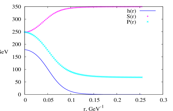
Figure 3: The critical bubble profile for the set $(1)$ in Table 2.

The points in Table 2 correspond to the strongly ($v_{c}/T_{c}>1$) first order phase transition.

Let us comment briefly on the applicability of the perturbation theory for the calculation of the effective potential $V_{T}$ near the critical temperature. Generally, the perturbation theory at finite temperature is plagued by IR divergences coming from the gauge and scalar sectors. The IR divergences in the gauge sector invalidate the perturbative calculations at $v=0$. However, the small magnetic mass (of order of $g^{2}T/\left(4\pi\right)$) of the gauge bosons is generated nonperturbatively, and it serves the infrared cutoff for the perturbation theory. It was shown in Ref. [26] that the effect of the magnetic mass renders the one-loop effective potential a good approximation even near $v=0$. This effect comes from the interaction of gauge bosons and in our model it is the same as in SM. As for scalar sector, the dimensionless expansion parameter $\delta_{T}$ for unresummed effective potential can be estimated as $\delta_{T}(v)=\tilde{\delta}T^{2}/6m^{2}_{T}(v)$ [27], where $m_{T}(v)$ is the smallest thermal mass of scalar particle (we do not show explicitly the dependence of $\delta_{T}$ on vev’s of singlet scalar fields) and $\tilde{\delta}$ is the corresponding coupling constant, which, for our parameter choice, is equal to $\tilde{\lambda}\sim 0.36$ (cf. eq. (35)). We have calculated the thermal mass and the expansion parameter at the critical temperature $T_{c}$ for both minima of the effective potential $V_{T}$ and present the results in the last two columns of Table 2. One concludes that the perturbation theory is applicable for the points in Table 2.

4 The baryon asymmetry

In this section we estimate the amount of the baryon asymmetry produced during the phase transition. There are several approaches to this problem (see, e.g., [28], [29], [30] and references therein). We have chosen to use the diffusion approximation for the description of the particle densities in the presence of moving bubble wall and WKB approximation for the CP-violating sources. We take into account CP-violation coming from chargino sector only. For the sake of simplicity, we ignore the singlino sector contribution to the diffusion equations leaving this for future study.

According to the semiclassical picture, particles and antiparticles have different dispersion relations in CP-violating background of the bubble wall [31]. Initially, the asymmetry in their densities emerges in the chargino sector and then, due to interactions and diffusion processes, it is transmitted into the densities of other particle species including left-handed fermions and, finally, to the baryon asymmetry.

We derive the diffusion equations along the lines of Ref. [32]. We describe the behaviour of the $i$-th type of particles by the currents $j_{i\mu}=\left(n_{i},\vec{j}_{i}\right)$, where $n_{i}$ is the particle density and $\vec{j}_{i}$ is the current density. In the diffusion approximation the current densities have the form $\vec{j}_{i}=-D_{i}\vec{\nabla}n_{i}$, where $D_{i}$ are diffusion constants, so diffusion equations can be written in the form

$$\dot{n}_{i}-D_{i}{\bf\nabla}^{2}n_{i}=I_{i}\;.$$ (48)

Here the dot denotes the time derivative, $I_{i}$ are source terms to be described below. To the linear order in chemical potentials $\mu_{i}$, one has

$$n_{i}=g_{i}\int\frac{d^{3}k}{(2\pi)^{3}}\left[f(E_{i},\mu_{i})-f(E_{i},-\mu_{i})\right]=\frac{k_{i}(m_{i}/T)T^{2}}{6}\mu_{i},$$ (49)

where $g_{i}$ is the number of degrees of freedom, $f(E_{i},\mu_{i})$ is boson (or fermion) distribution function, factor $k_{i}(m_{i}/T)$ is equal to $2$ ($1$) for one boson (fermion) massless degree of freedom ($m_{i}=0$) and is exponentially suppressed in the limit $m_{i}/T\to\infty$.

First, we neglect CP-violating reactions and weak sphalerons. The CP-conserving part of the source terms can be written (again, to linear order in chemical potentials) as follows,

$$I_{i}=\sum_{r}\Gamma^{r}_{i}\sum_{k}\mu_{k},$$ (50)

where the first sum runs over all reactions with the rate $\Gamma^{r}_{i}$, in which the $i$-th type of particles participates, and the second sum runs over all types of particle species participating in the $r$-th reaction. As an example, for the process $A+2B\to C+3D$ with rate $\Gamma$ the corresponding term for particle $A$ is $I_{A}\supset-\Gamma_{A}\left(\mu_{A}+2\mu_{B}-\mu_{C}-3\mu_{D}\right)$.

We neglect all Yukawa interactions except for the top quark. Then, leptons do not participate in the processes of diffusion of the particle-antiparticle asymmetry. Moreover, strong sphalerons, induced by the operator $\prod_{i=1}^{3}\bar{u}_{Ri}u_{Li}\bar{d}_{Ri}d_{Li}$, where index $i$ runs over three generations of quarks, are the only processes which produce light quarks; therefore, one algebraically constrains the quark densities as follows,

$$n_{Q_{1}}=n_{Q_{2}}=-2n_{u_{R}}=-2n_{d_{R}}=-2n_{s_{R}}=-2n_{c_{R}}=-2n_{B},$$ (51)

where $n_{Q_{i}}\equiv n_{u_{Li}}+n_{d_{Li}}$, ($i=1,2,3$) are the densities of left doublets and $n_{B}\equiv n_{b_{R}}$. The conservation of the baryon number, along with aforementioned constraints, results in $n_{B}+n_{T}+n_{Q}=0$, where we use the standard notations $n_{T}\equiv n_{t_{R}}$ and $n_{Q}\equiv n_{Q_{3}}$.

Since we neglect the singlet sector contribution, we only write down the source terms for the Higgs doublet $H^{\prime}=\left(H^{+},H^{0}\right)^{T}$ (we use prime here to save the notation $H$ for later use), higgsinos $\tilde{H}_{u}=\left(\tilde{H}_{u}^{+},\tilde{H}_{u}^{0}\right)^{T}$, $\tilde{H}_{d}=\left(\tilde{H}_{d}^{0},\tilde{H}_{d}^{-}\right)^{T}$ and heavy quarks $Q=(t_{L},b_{L})^{T}$, $t_{R}$ and $b_{R}$ . The gauge interactions are assumed to be in equilibrium, so the chemical potentials of the gauge bosons are equal to zero. Therefore, the chemical potentials of the particles in $SU(2)_{L}$ doublets are equal and, for our purposes, it is sufficient to consider only the sums of densities $n_{Q}=n_{t_{L}}+n_{b_{L}}$, $n_{H^{\prime}}=n_{H^{+}}+n_{H^{0}}$, $n_{\tilde{H}_{u}}=n_{\tilde{H}_{u}^{+}}+n_{\tilde{H}_{u}^{0}}$ and $n_{\tilde{H}_{d}}=n_{\tilde{H}_{d}^{0}}+n_{\tilde{H}_{d}^{-}}$. We also make usual assumptions, that the chemical potentials of winos and bino are zero, being driven by the high rate of helicity flipping interactions induced by their Majorana mass terms.

The following interactions are considered in the diffusion equations:

(i) strong sphalerons with the rate $\Gamma_{ss}=6\kappa_{ss}\frac{8}{3}\alpha_{s}^{4}T$, where $\kappa_{ss}=O(1)$ [32],

(ii) top quark Yukawa interactions $y_{t}\bar{Q}tH$ with the rate $\Gamma_{Y}$,

(iii) interactions due to the term $\tilde{\mu}\tilde{H}_{u}\epsilon\tilde{H}_{d}$ with the rate $\Gamma_{\mu}$,

(iv) top quark mass effects with the rate $\Gamma_{m}$,

(v) Higgs boson self interactions with the rate $\Gamma_{H}$,

(vi) Higgs-higgsino-gaugino interactions with the rates $\Gamma_{u}$ and $\Gamma_{d}$ for up and down higgsino doublets, respectively.

We neglect the curvature of the bubble wall and suppose that the main part of the baryon asymmetry is produced when the bubble expands already in the stationary regime. It means that near the wall all space-time dependent quantities should depend only on the combination $z+v_{w}t$, where $v_{w}$ is the bubble wall velocity and $z$ is a coordinate along the axis, perpendicular to the wall, whose positive direction points to the broken phase. In particular, $n_{i}\left(\vec{r},t\right)=n_{i}\left(z+v_{w}t\right)$ and hence $\dot{n}_{i}=v_{w}n_{i}$.

With above assumptions one writes the diffusion equations as follows

$$v_{w}n_{Q}^{\prime}-D_{q}n_{Q}^{\prime\prime} = -\left(\mu_{Q}-\mu_{T}-\mu_{H^{\prime}}\right)\Gamma_{Y}-\left(\mu_{Q}-\mu_{T}\right)\Gamma_{m}$$

$$-6\left(2\mu_{Q}-\mu_{T}+9\mu_{B}\right)\Gamma_{ss},$$

$$v_{w}n_{T}^{\prime}-D_{q}n_{T}^{\prime\prime} = \left(\mu_{Q}-\mu_{T}-\mu_{H^{\prime}}\right)\Gamma_{Y}+\left(\mu_{Q}-\mu_{T}\right)\Gamma_{m}$$

$$+3\left(2\mu_{Q}-\mu_{T}+9\mu_{B}\right)\Gamma_{ss},$$

$$v_{w}n_{H^{\prime}}^{\prime}-D_{h}n_{H^{\prime}}^{\prime\prime} = -\left(\mu_{H^{\prime}}-\mu_{Q}+\mu_{T}\right)\Gamma_{Y}-\left(\mu_{H^{\prime}}-\mu_{\tilde{H}_{u}}\right)\Gamma_{u}$$

$$-\left(\mu_{H^{\prime}}+\mu_{\tilde{H}_{d}}\right)\Gamma_{d}-\mu_{H^{\prime}}\Gamma_{H},$$

$$v_{w}n_{\tilde{H}_{u}}^{\prime}-D_{h}n_{\tilde{H}_{u}}^{\prime\prime} = -\left(\mu_{\tilde{H}_{u}}-\mu_{H^{\prime}}\right)\Gamma_{u}-\left(\mu_{\tilde{H}_{u}}+\mu_{\tilde{H}_{d}}\right)\Gamma_{\mu}+S_{u},$$ (55)

$$v_{w}n_{\tilde{H}_{d}}^{\prime}-D_{h}n_{\tilde{H}_{d}}^{\prime\prime} = -\left(\mu_{\tilde{H}_{d}}+\mu_{H^{\prime}}\right)\Gamma_{d}-\left(\mu_{\tilde{H}_{u}}+\mu_{\tilde{H}_{d}}\right)\Gamma_{\mu}+S_{d},$$ (56)

where it is also assumed that the diffusion constants $D_{q}$ are the same for all quarks and $D_{h}$ for all higgses and higgsinos. Here we include CP-violating sources $S_{u}$ and $S_{d}$, which we describe later. Neglecting moderate RG effects one estimates the ratio $\Gamma_{u}/\Gamma_{d}=\tan^{2}{\beta}$. We consider the limit of large $\tan{\beta}$, when $\Gamma_{u}\gg\Gamma_{d}$, and assume the interactions corresponding to the rate $\Gamma_{u}$ to be in equilibrium, which implies the constraint $\mu_{H^{\prime}}-\mu_{\tilde{H}_{u}}=0$. Introducing the notation $\Gamma_{\tilde{\mu}}\equiv\Gamma_{\mu}+\Gamma_{d}$ and excluding the terms with $\Gamma_{u}$ from eqs. (4), (55), one can write down the following linear combinations

$$I_{H^{\prime}}+I_{\tilde{H}_{u}} = -\left(\mu_{H^{\prime}}-\mu_{Q}+\mu_{T}\right)\Gamma_{Y}-\left(\mu_{H^{\prime}}+\mu_{H_{d}}\right)\Gamma_{\tilde{\mu}}-\mu_{H^{\prime}}\Gamma_{H}+S_{d},$$ (57)

$$I_{\tilde{H}_{d}} = -\left(\mu_{H_{d}}+\mu_{H^{\prime}}\right)\Gamma_{\tilde{\mu}}+S_{u}.$$ (58)

Upon defining the densities

$$n_{h}=n_{H^{\prime}}+n_{\tilde{H}_{u}}+n_{\tilde{H}_{d}},\;\;n_{H}=n_{H^{\prime}}+n_{\tilde{H}_{u}}-n_{\tilde{H}_{d}},\;\;$$

we obtain the following set of diffusion equations

$$v_{w}n_{Q}^{\prime} = D_{q}n^{\prime\prime}_{Q}-\Gamma_{Y}\left[\frac{n_{Q}}{k_{Q}}-\frac{n_{T}}{k_{T}}-\frac{n_{H}+n_{h}}{k_{H_{1}}}\right]-\Gamma_{m}\left[\frac{n_{Q}}{k_{Q}}-\frac{n_{T}}{k_{T}}\right]$$

$$-6\Gamma_{ss}\left[2\frac{n_{Q}}{k_{Q}}-\frac{n_{T}}{k_{T}}+9\frac{n_{Q}+n_{T}}{k_{B}}\right],$$

$$v_{w}n_{T}^{\prime} = D_{q}n_{T}^{\prime\prime}+\Gamma_{Y}\left[\frac{n_{Q}}{k_{Q}}-\frac{n_{T}}{k_{T}}-\frac{n_{H}+n_{h}}{k_{H_{1}}}\right]+\Gamma_{m}\left[\frac{n_{Q}}{k_{Q}}-\frac{n_{T}}{k_{T}}\right]$$

$$+3\Gamma_{ss}\left[2\frac{n_{Q}}{k_{Q}}-\frac{n_{T}}{k_{T}}+9\frac{n_{Q}+n_{T}}{k_{B}}\right],$$

$$v_{w}n_{H}^{\prime} = D_{h}n_{H}^{\prime\prime}+\Gamma_{Y}\left[\frac{n_{Q}}{k_{Q}}-\frac{n_{T}}{k_{T}}-\frac{n_{H}+n_{h}}{k_{H_{1}}}\right]-\Gamma_{H}\frac{n_{H}+n_{h}}{k_{H_{1}}}+S_{u}-S_{d},$$ (61)

$$v_{w}n_{h}^{\prime} = D_{h}n_{h}^{\prime\prime}+\Gamma_{Y}\left[\frac{n_{Q}}{k_{Q}}-\frac{n_{T}}{k_{T}}-\frac{n_{H}+n_{h}}{k_{H_{1}}}\right]-2\left[\frac{n_{H}}{k_{H}}+\frac{n_{h}}{k_{h}}\right]\Gamma_{\tilde{\mu}}$$

$$-\frac{n_{H}+n_{h}}{k_{H_{1}}}\Gamma_{H}+S_{u}+S_{d},$$

where

$$k_{H_{1}}=2(k_{H^{\prime}}+k_{\tilde{H}_{u}}),\;\;\;k_{H}=\frac{2(k_{H^{\prime}}+k_{\tilde{H}_{u}})k_{\tilde{H}_{d}}}{k_{\tilde{H}_{d}}-k_{H^{\prime}}-k_{\tilde{H}_{u}}},\;\;\;k_{h}=\frac{2(k_{H^{\prime}}+k_{\tilde{H}_{u}})k_{\tilde{H}_{d}}}{k_{\tilde{H}_{d}}+k_{H^{\prime}}+k_{\tilde{H}_{u}}}.\;\;$$

We note in passing that in the case $\tan{\beta}\sim 1$, the assumption, that $\Gamma_{u}$ and $\Gamma_{d}$ are in equilibrium leads to a single diffusion equation for $n_{H}$, which is sourced only by the difference $S_{u}-S_{d}$. As we will discuss later, in the semiclassical limit $S_{u}=S_{d}$, hence no baryon asymmetry is produced, however, other approaches to the calculation of the CP-violating sources, see, e.g., [29, 34, 35]) can lead to non-zero difference $S_{u}-S_{d}$.

Making standard assumption that strong sphaleron and Yukawa interactions are in equilibrium and follow procedure described in Ref. [29], we find the relations

$$n_{T}=-\frac{k_{T}\left(2k_{B}+9k_{Q}\right)}{k_{H_{1}}\left(9k_{Q}+9k_{T}+k_{B}\right)}\left(n_{H}+n_{h}\right),\;\;n_{Q}=\frac{k_{Q}\left(9k_{T}-k_{B}\right)}{k_{H_{1}}\left(9k_{Q}+9k_{T}+k_{B}\right)}\left(n_{H}+n_{h}\right)$$ (63)

and the equations for densities $n_{H}$ and $n_{h}$

$${\bf\mathcal{A}}\left(\begin{array}[]{c}n_{H}^{\prime}\\ n_{h}^{\prime}\end{array}\right)={\bf D}\left(\begin{array}[]{c}n_{H}^{\prime\prime}\\ n_{h}^{\prime\prime}\end{array}\right)-{\bf\mathcal{G}}\left(\begin{array}[]{c}n_{H}\\ n_{h}\end{array}\right)+{\bf S},$$ (64)

where

$$\begin{split}{\bf\mathcal{A}}=\left(\begin{array}[]{cc}1&\frac{F}{F+G}\\ \frac{F}{F+G}&1\end{array}\right),\;\;{\bf D}=\left(\begin{array}[]{cc}\bar{D}_{q}+\bar{D}_{h}&\bar{D}_{q}\\ \bar{D}_{q}&\bar{D}_{q}+\bar{D}_{h}\end{array}\right),\;\;\\ {\bf\mathcal{G}}=\left(\begin{array}[]{cc}\bar{\Gamma}_{m}+\bar{\Gamma}_{h}&\bar{\Gamma}_{m}+\bar{\Gamma}_{h}\\ \bar{\Gamma}_{m}+\bar{\Gamma}_{h}+2\bar{\Gamma}_{\tilde{\mu}}&\bar{\Gamma}_{m}+\bar{\Gamma}_{h}+2\frac{k_{H}}{k_{h}}\bar{\Gamma}_{\tilde{\mu}}\end{array}\right),\;\;{\bf S}=\left(\begin{array}[]{c}\frac{G}{G+F}\left(S_{u}+S_{d}\right)\\ \frac{G}{G+F}\left(S_{u}-S_{d}\right)\end{array}\right),\end{split}$$ (65)

where $\bar{\Gamma}_{i}=\frac{G}{G+F}\Gamma_{i}$, $\bar{D}_{q}=\frac{F}{F+G}D_{q}$, $\bar{D}_{h}=\frac{G}{F+G}D_{h}$ and

$$F=9k_{Q}k_{T}+k_{Q}k_{B}+4k_{T}k_{B},\;\;G=k_{H_{1}}\left(9k_{Q}+9k_{T}+k_{B}\right).$$

Using (63), one finds the density of left-handed fermions

$$n_{Left}=n_{Q_{1}}+n_{Q_{2}}+n_{Q_{3}}=4n_{T}+5n_{Q}\\ =\frac{5k_{Q}k_{B}+8k_{T}k_{B}-9k_{Q}k_{T}}{k_{H_{1}}\left(k_{B}+9k_{Q}+9k_{T}\right)}\left(n_{h}+n_{H}\right)\equiv A\cdot(n_{h}+n_{H}).$$ (66)

For our set of statistical factors ($k_{Q}=6,\;k_{T}=3,\;k_{B}=3$, $k_{H^{\prime}}=4,\;k_{\tilde{H}_{u}}=k_{\tilde{H}_{d}}=2$ in the massless case), which is the same as in SM (except for the higgsino sector), the value of constant $A$ equals zero. This is well known Standard Model suppression [36]. As shown in Ref. [14] for similar situation, the corrections due to subleading $O(1/\Gamma_{ss})$ effects are small, while radiative corrections to the thermal masses of particles give a sizable contribution mainly due to the top Yukawa coupling,

$$A=\frac{3}{2k_{H_{1}}}\left(-\frac{3y_{t}^{2}}{8\pi^{2}}\right).$$ (67)

The space-time distribution of left-handed fermions acts as a source for baryon asymmetry [29], which obeys the following equation

$$v_{w}n_{B}^{\prime}(z)=-\theta(-z)\left[n_{F}\Gamma_{ws}n_{Left}(z)+{\cal R}n_{B}\right],$$ (68)

where $\Gamma_{ws}$ is the weak sphaleron rate ($\Gamma_{ws}=6\kappa_{ws}\alpha_{w}^{5}T$, where $\kappa_{ws}=20\pm 2$ [37]), ${\cal R}$ is the relaxation coefficient [28, 38] (${\cal R}=\frac{5}{4}n_{F}\Gamma_{ws}$), and $n_{F}=3$ is the number of families. Here theta-function implies that the weak sphalerons are active only in the unbroken phase. The solution of this equation can be obtained analytically, and the resulting baryon asymmetry takes the form

$$n_{B}=-\frac{n_{F}\Gamma_{ws}}{v_{w}}\int_{-\infty}^{0}dzn_{Left}(z)e^{z{\cal R}/v_{w}}.$$ (69)

In the WKB approximation, the source terms $S_{u}$ and $S_{d}$ are derived from chargino dispersion relations. The mass matrix of charginos reads as follows,

$$M_{ch}=\left(\begin{array}[]{cc}M_{2}&\frac{1}{\sqrt{2}}\tilde{g}_{u}h(z)\\ \frac{1}{\sqrt{2}}\tilde{g}_{d}h(z)&\tilde{\mu}(z)\end{array}\right),$$ (70)

where we introduce the notation $\tilde{\mu}(z)=\mu+\kappa\left(S(z)+iP(z)\right)/\sqrt{2}$. The expressions for the sources (up to overall factor) come from Ref. [8], where it has been shown that, in fact, the CP-violating sources for higgsinos $\tilde{H}_{u}$ and $\tilde{H}_{d}$ are equal, so only the equation for density $n_{h}$ is sourced. The expressions for the sources read

$$S_{u}=S_{d}=\frac{T^{2}D_{h}v_{w}}{6\langle p_{z}^{2}/E\rangle_{0}}\Big{\{}\langle A\rangle\big{[}\theta^{\prime}-\gamma^{\prime}\sin^{2}{a}+\delta^{\prime}\sin^{2}{b}\big{]}^{\prime}+\\ \langle B\rangle(m_{\tilde{h}}^{2})^{\prime}\big{[}\theta^{\prime}-\gamma^{\prime}\sin^{2}{a}+\delta^{\prime}\sin^{2}{b}\big{]}\Big{\}}^{\prime},$$ (71)

where

$$\langle A\rangle=\left\langle\frac{|p_{z}||m_{\tilde{h}}|^{2}}{2E^{2}}\right\rangle_{+},\;\;\;\langle B\rangle=\left\langle\frac{|p_{z}|(E^{2}-|m_{\tilde{h}}|^{2})}{2E^{4}}\right\rangle_{+},$$ (72)

and $E^{2}={\bf p}^{2}+m_{\tilde{h}}^{2}$, $p_{z}$ is the component of the spatial momentum perpendicular to the wall, and $m_{\tilde{h}}$ is the mass eigenstate of the matrix (70), which becomes pure higgsino in the unbroken phase. The thermal averages $\langle\;\rangle_{+}$ and $\langle\;\rangle_{0}$ are performed with fermion distribution function

$$\langle A\left(\vec{p}\right)\rangle=\frac{\int d^{3}p\left(df/dE\right)A\left(\vec{p}\right)}{\int d^{3}p\left(df/dE\right)|_{m=0}},\;\;\;\frac{df}{dE}=-\beta\frac{{\rm e}^{\beta E}}{\left({\rm e}^{\beta E}+1\right)^{2}}$$ (73)

for massive $(+)$ and massless $(0)$ cases, respectively. The other quantities in eq. (71) come from the diagonalization of chargino mass matrix [8],

$$\sin^{2}a=2|A|^{2}/\Lambda(\Lambda+\Delta),\;\;\;A=h\left(\tilde{g}_{u}M_{2}+\tilde{g}_{d}\tilde{\mu}\right)/\sqrt{2},\;\;\;\Lambda=\left(\Delta^{2}+4|A|^{2}\right)^{1/2},$$ (74)

$$\gamma={\rm arg}A,\;\;\;\gamma^{\prime}\sin^{2}{a}=2{\rm Im}\left(A^{*}A^{\prime}\right)/\Lambda\left(\Lambda+\Delta\right),\;\;\;\Delta=M_{2}^{2}-|\tilde{\mu}|^{2}+\left(\tilde{g}_{d}^{2}-\tilde{g}_{u}^{2}\right)h^{2}$$ (75)

The expressions for $\sin^{2}{b}$, $\delta$ and $\delta^{\prime}\sin^{2}{b}$ are obtained from the ones for $\sin^{2}{a}$, $\gamma$ and $\gamma^{\prime}\cos^{2}{a}$ by replacement $a\to b$, $\tilde{g}_{u}\to\tilde{g}_{d}$ and $\gamma\to-\delta$.

To calculate CP-violating sources, we need the bubble wall profile. The standard way to find it is to solve the equations of motion, derived from the effective potential $V_{T}(h,S,P)$ at the critical temperature $T_{c}$ (for recent calculations of the bubble wall profiles in (N)MSSM see, e.g., Refs. [24]). For our purposes we approximate its form by the standard kink-like solution

$$h(z)=\frac{1}{2}v_{c}\left(1-\tanh{\left[\alpha\left(1-\frac{2z}{L_{w}}\right)\right]}\right),$$ (76)

$$\left(\begin{array}[]{c}S(z)\\ P(z)\\ \end{array}\right)=\left(\begin{array}[]{c}S_{c}\\ P_{c}\\ \end{array}\right)-\frac{1}{2}\left(\begin{array}[]{c}\Delta v_{S}\\ \Delta v_{P}\\ \end{array}\right)\left(1+\tanh{\left[\alpha\left(1-\frac{2z}{L_{w}}\right)\right]}\right),$$ (83)

where $S_{c}$, $P_{c}$ are the critical values of the singlet scalar fields, $\Delta v_{S}=S_{c}-S_{s}$ and $\Delta v_{P}=P_{c}-P_{s}$ (see also Table 2), $L_{w}$ is the bubble wall width, which is taken to be the same for all scalar fields, and the constant $\alpha$ is taken to be $1.5$ as in Ref. [29]. Here we have assumed that at $z>L_{w}/(2\alpha)$ gauge symmetry is broken (the inner region of the bubble) and at $z<0$ symmetry is restored (outer region).

For numerical calculations we take the diffusion constants to be $D_{q}\sim 6/T$ for quarks and $D_{h}\sim 110/T$ for Higgs sector [33]; the width and the velocity of the bubble wall are taken as $L_{w}=8.0/T$ and $v_{w}=0.1$, respectively. The rates

$$\Gamma_{H}=0.0036T\;\theta\left(z-0.5L_{w}\right),\;\;\;\Gamma_{m}=0.05T\;\theta\left(z-0.5L_{w}\right)$$ (84)

are the same as in Ref. [8] and $\Gamma_{\tilde{\mu}}=0.1T$ [7].

Below we present the results for the baryon-to-entropy ratio $\Delta=n_{B}/s$ with entropy density $s$ given by $s=2\pi^{2}g_{eff}T^{3}/45,$ where $g_{eff}$ is the effective number of relativistic degrees of freedom at the critical temperature. We plot the ratio $\Delta/\Delta_{0}$, where $\Delta_{0}=8.7\cdot 10^{-11}$, which corresponds to $n_{B}/n_{\gamma}=6.5\cdot 10^{-10}$ (cf. eq. (1)). In Fig. 4

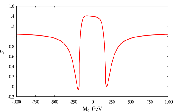
Figure 4: Plot of $\Delta/\Delta_{0}$ as a function of $M_{2}$ for the set $(2)$ of parameters presented in Table 2.

we show the dependence of the baryon asymmetry on the gaugino mass $M_{2}$ for the set $(2)$ of the parameters in the Tables 1 and 2. We found that in contrast to MSSM, the baryon asymmetry does not vanish in the limit of infinite $M_{2}$, where one of the chargino species decouples. This fact may be attributed to the strong $z$-dependence of the effective $\tilde{\mu}$ parameter. We have checked numerically that in the limits $M_{2}\to+\infty$ and $M_{2}\to-\infty$ the results for the baryon asymmetry coincide as it should be, since in both cases charged gaugino (wino) is very heavy and does not affect the low energy physics. Similarly, at $|M_{2}|<<|\tilde{\mu}|$ the amount of baryon asymmetry is not very sensitive to $M_{2}$ and is determined by $\tilde{\mu}(z)$ and off-diagonal entries of the mass matrix (70). In both regions ($M_{2}\to\infty$ and $M_{2}\to 0$) wino admixture in the relevant higgsino-like mass eigenstate is small, so our approximation where we neglect mixing in diffusion equations can be justified. The region of large higgsino-wino mixing ($|M_{2}|\sim|\tilde{\mu}|\sim 200$ GeV in Figure 4) should be considered more accurately if one wants to know the exact amount of baryon asymmetry produced in this case (see [30] and references therein).

To summarize this section, we demonstrated that the model is indeed capable of producing sufficient amount of the baryon asymmetry. There are certainly values of parameters for which the electroweak phase phase transition is sufficiently strongly first order, and electroweak baryogenesis is sufficiently efficient. In this analysis we restricted ourselves to rather small range of parameters. It remains to be understood how generic is successive electroweak baryogenesis in the whole parameter space.

5 Electric dipole moments

One of the consequences of the presence of additional sources of CP-violation is their contribution to the electron and neutron EDMs. Like in the minimal split SUSY model, there are three types of contributions to EDM of a fermion (lepton or quark), related to the exchange of $h_{0}\gamma$, $W^{+}W^{-}$ and $h_{0}Z$ bosons (see Refs. [39], [40], [41], [42]). The corresponding two-loop Feynman diagrams for SM fermion $f$ (charged lepton or quark) are given in Fig. 5.

Figure 5: Feynman diagrams contributing to the fermion EDM in split SUSY.

It was shown in Ref. [42] that the third contribution is suppressed in the case of electron by a factor ($1-4\sin^{2}{\theta_{W}}$), where $\theta_{W}$ is the weak mixing angle, while it is important for the neutron EDM. In the minimal split SUSY model there is only one CP-violating phase, associated with the invariant $\phi_{1}={\rm arg}(\tilde{g_{u}}^{*}\tilde{g_{d}}^{*}M_{2}\tilde{\mu})$ where $\tilde{\mu}=\mu+\kappa\left(v_{S}+iv_{P}\right)/\sqrt{2}$. In the class of models presented here, among parameters directly governing the couplings contributing to the diagrams in Fig. 5, two additional independent phases appear, which correspond to the phase invariants $\phi_{2}={\rm arg}\left(\kappa k^{*}\lambda_{u}\lambda_{d}(\tilde{\mu}^{*})^{-2}\right)$ and $\phi_{3}={\rm arg}\left(\lambda_{u}\lambda_{d}^{*}\tilde{g}_{u}^{*}\tilde{g}_{d}\right)$.

After diagonalization of chargino and neutralino mass matrices, the relevant part of the interaction Lagrangian becomes

$${-\cal L_{\rm{int}}}=\frac{g}{\cos_{\theta_{W}}}\bar{\chi}_{i}^{+}\gamma^{\mu}\left(G^{R}_{ij}P_{R}+G_{ij}^{L}P_{L}\right)\chi_{j}^{+}Z_{\mu}$$ (85)

$$+\left[g\bar{\chi}^{+}_{i}\gamma^{\mu}\left(C_{ij}^{R}P_{R}+C_{ij}^{L}P_{L}\right)\chi_{j}^{0}W_{\mu}^{+}+\frac{g}{\sqrt{2}}\bar{\chi}_{i}^{+}\left(D_{ij}^{R}P_{R}+D_{ij}^{L}P_{L}\right)\chi_{j}^{+}h+h.c.\right],$$

where the matrices are

$$G_{ij}^{L}=V_{i1}c_{W^{+}}V^{\dagger}_{1j}+V_{i2}c^{h_{u}^{+}}V^{\dagger}_{2j},\;\;-G_{ij}^{R*}=U_{i1}c_{W^{-}}U^{\dagger}_{1j}+U_{i2}c_{h_{d}^{-}}U^{\dagger}_{2j},$$ (86)

$$gD_{ij}^{R}=\tilde{g}^{*}_{u}V_{i2}U_{j1}+\tilde{g}^{*}_{d}V_{i1}U_{j2},\;\;gD^{L}=\left(gD^{R}\right)^{\dagger},$$ (87)

with $i,j=1,2$ and $c_{W^{\pm}}=\pm\cos^{2}{\theta_{W}}$, $c_{h_{u}^{+},h_{d}^{-}}=\pm(1/2-\sin^{2}{\theta_{W}})$,

$$C_{ij}^{L}=-V_{i1}N^{*}_{j2}+\frac{1}{\sqrt{2}}V_{i2}N^{*}_{j4},\;\;C_{ij}^{R}=-U^{*}_{i1}N_{j2}-\frac{1}{\sqrt{2}}U^{*}_{i2}N_{j3},\;\;$$ (88)

with $i=1,2$ and $j=1,\dots,5$. Here the unitary matrices $V$, $U$ and $N$ diagonalize the mass matrix of charginos (70) and the mass matrix of neutralinos

$$M_{n}=\left(\begin{array}[]{ccccc}M_{1}&0&-\frac{1}{2}\tilde{g}^{\prime}_{d}v&\frac{1}{2}\tilde{g}^{\prime}_{u}v&0\\ 0&M_{2}&\frac{1}{2}\tilde{g}_{d}v&\frac{1}{2}\tilde{g}_{u}v&0\\ -\frac{1}{2}\tilde{g}^{\prime}_{d}v&\frac{1}{2}\tilde{g}_{d}v&0&-\tilde{\mu}&\frac{1}{\sqrt{2}}\lambda_{d}v\\ \frac{1}{2}\tilde{g}^{\prime}_{u}v&\frac{1}{2}\tilde{g}_{u}v&-\tilde{\mu}&0&\frac{1}{\sqrt{2}}\lambda_{u}v\\ 0&0&\frac{1}{\sqrt{2}}\lambda_{d}v&\frac{1}{\sqrt{2}}\lambda_{u}v&-\sqrt{2}k(v_{S}+iv_{P})\end{array}\right)$$ (89)

so that $U^{*}{\cal M}_{C}V^{\dagger}={\rm diag}(m_{\chi^{+}_{1}},m_{\chi^{+}_{2}})$ and $N^{*}{\cal M}N^{\dagger}={\rm diag}(m_{\chi^{0}_{1}},m_{\chi^{0}_{2}},m_{\chi^{0}_{3}},m_{\chi^{0}_{4}},m_{\chi^{0}_{5}})$. The EDM of electron or light quark has the form

$$d_{f}=d_{f}^{h\gamma}+d_{f}^{hZ}+d_{f}^{WW},$$

where expressions for the corresponding contributions can be found in Ref. [42]. We modified them appropriately in our case, because of different number of neutralinos. The neutron dipole moment can be expressed in terms of quark EDMs by the relation [43, 44]

$$d_{n}=(1\pm 0.5)\left[\frac{f_{\pi}^{2}m_{\pi}^{2}}{(m_{u}+m_{d})(225{\rm MeV})^{3}}\right]\left(\frac{4}{3}d_{d}-\frac{1}{3}d_{u}\right),$$ (90)

where $f_{\pi}=92$ MeV and $m_{u}/m_{d}=0.55$.

For numerical calculations we use two sets of parameters (see Table 1) and randomly scan over the following parameter space, $0<M_{1},M_{2}<1000$ GeV. Also we take the coupling $k$ to be complex, $k=|k|e^{i\phi_{k}}$, ($0<\phi_{k}<\pi$) to include the contribution of the phase invariant $\phi_{2}$. The results for the electron and neutron EDMs as functions of the mass of the lightest chargino are presented in Figs. 6 and 7, respectively. We have taken into account the experimental bound on the mass of the lightest chargino $m_{\chi^{+}}>104$ GeV [45].

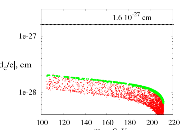
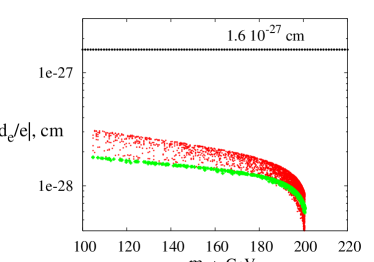
Figure 6: The EDM of electron as a function of the mass of the lightest chargino $m_{\chi^{+}}$ for set 1 (left) and set 2 (right) of parameters in Table 1. Horizontal dotted line represents the experimental bound $|d_{e}|<1.6\cdot 10^{-27}{\rm e\;cm}$. Green (gray) points represent the values of EDM for real $k$.

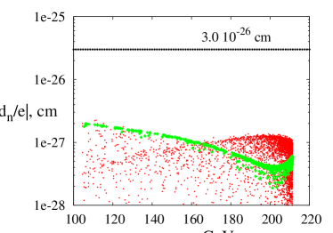
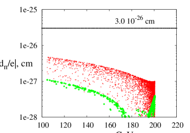
Figure 7: The EDM of neutron as a function of the mass of the lightest chargino $m_{\chi^{+}}$ for the same sets of parameters as in Fig. 6. Horizontal line represents the experimental bound $|d_{n}|<3.0\cdot 10^{-26}{\rm e\;cm}$. Green (grey) points represent the values of EDM for real $k$.

Horizontal lines show the present experimental limit on the EDM of electron $|d_{e}|<1.6\cdot 10^{-27}$ e cm at $90$% CL [46] and neutron $|d_{n}|<3.0\cdot 10^{-26}$ e cm at $90$% CL [47]. One observes that generally for the cosmologically favorable models, the predictions for EDMs are within one-two orders of magnitude below the present experimental bound. Hence, our solution of the baryon asymmetry problem can be indirectly probed by the future experiments aimed at EDM searches.

6 Dark matter candidates

In this section we explore dark matter in the model. In the minimal split SUSY this issue has been already investigated in Refs. [12], [39], [48]. In the first place, let us note that a generalization of R-parity can be introduced in the nonminimal split SUSY: with respect to this R-parity all new fermionic fields are odd, while new (pseudo)scalars are even. Hence the lightest new fermion is the lightest superpartner and it is stable.

The viable dark matter particles should be electrically neutral, so the best candidates in our model are neutralinos. We define the LSP neutralino state as

$$\chi=N_{51}\tilde{B}+N_{52}\tilde{W}+N_{53}\tilde{H}_{u}+N_{54}\tilde{H}_{d}+N_{55}\tilde{n}.$$ (91)

We estimate the neutralino relic abundance by using the standard methods [49]. First we calculate the freeze-out temperature $T_{F}$,

$$x_{F}={\rm log}\left(\frac{m_{\chi}}{2\pi^{3}}\sqrt{\frac{45}{2g_{*}G_{N}x_{F}}}\langle\sigma v\rangle_{\rm M\o l}\right),$$ (92)

where $x_{F}=m_{\chi}/T_{F}$, $g_{*}$ is the effective number of degrees of freedom at freeze-out $g^{1/2}_{*}\sim 9$; the thermally-averaged product of neutralino annihilation cross section $\sigma$ and relative velocity $v$ of neutralinos (the Møller cross section $\langle\sigma v\rangle_{\rm M\o l}$) is

$$\langle\sigma v\rangle_{\rm M\o l}=\frac{1}{8m_{\chi}^{4}TK_{2}^{2}(m_{\chi}/T)}\int_{4m_{\chi}^{2}}^{\infty}ds\sigma(s)(s-4m_{\chi}^{2})\sqrt{s}K_{1}\left(\frac{\sqrt{s}}{T}\right).$$ (93)

Here $K_{1}$, $K_{2}$ are the modified Bessel functions, $s$ is the Mandelstam variable. The relic abundance of the lightest neutralino is then given by

$$\Omega_{\chi}h^{2}=\frac{(1.07\times 10^{9}{\rm GeV}^{-1})}{M_{Pl}}\left(\int_{x_{F}}^{\infty}dx\frac{\langle\sigma v\rangle_{\rm M\o l}(x)}{x^{2}}g_{*}^{1/2}\right)^{-1}.$$ (94)

To calculate the neutralino abundance, we modify the formulas for the annihilation cross sections presented in Ref. [50]. The changes concern the annihilation of neutralinos into the Higgs bosons and are due to new Feynman diagrams with singlet scalar and pseudoscalar exchanges in s-channel. The corresponding modifications are presented in Appendix B. The total number of neutralinos has been also changed according to our model.

Adopting constraints discussed in Sec. 2, we first scan uniformly over the following parameter space: $|M_{1}|$, $|M_{2}|<1000$ GeV, $|v_{P}|<2000$ GeV, with $v_{S}$ being in the region of correct electroweak vacuum (i.e. the electroweak breaking minimum is the global minimum of the potential) and squared mass matrix of the scalar fields being diagonal. The numerical results are presented in the left plot in Fig. 8, where we show the region in $(m_{\chi^{+}},\;m_{\chi}$) plane favored by WMAP data: each point corresponds to a model in which neutralino abundance is within the range $0.094<\Omega_{DM}h^{2}<0.129$ [1]. To check that the baryon asymmetry and dark matter problems can be solved simultaneously, we also scan uniformly over the region in the parameter space preferred by electroweak baryogenesis (cf. Sec. 4); namely, we use $|M_{1}|,\;|M_{2}|<1000$ GeV, with other parameters corresponding to the set $(2)$ in Tables 1 and 2. Points in ($M_{1},\;M_{2}$) plane, which correspond to correct neutralino abundance, are shown on the right plot in Fig. 8.

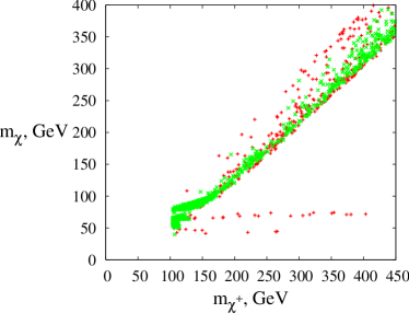
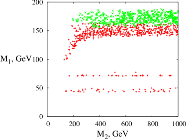
Figure 8: Points in ($m_{\chi^{+}}$, $m_{\chi}$) plane, i.e. the lightest chargino and the lightest neutralino (left) and in ($M_{2},\;M_{1}$) plane (right), which correspond to models with the correct relic abundance of singlino ($|N_{55}|>0.5$, green (light grey) oblique crosses) and non-singlino (red / dark grey crosses) dark matter.

On both plots green (light grey) crosses correspond to the dark matter particles which have considerable admixture of singlino ($|N_{55}|>0.5$), while the red (dark grey) crosses correspond to the mostly bino LSP. The annihilation of DM particles (bino as well as singlino) with masses $m_{\chi}\sim 0.5M_{h}\sim 75~{}$GeV or $m_{\chi}\sim 0.5M_{Z}$ proceeds resonantly via Higgs or $Z^{0}$-boson exchange, respectively. On the right plot, this light neutralino corresponds to the red (dark grey) horizontal lines with $M_{1}<80$ GeV. The most part of the parameter space with singlino-like dark matter give relatively light LSP with mass in the range $50-200$ GeV although heavier candidates are not entirely excluded. We have found that in this case, considerable admixture of higgsinos is always present (numerically, we obtain $\left(|N_{53}|^{2}+|N_{54}|^{2}\right)^{(1/2)}\sim 0.4-0.8$). Singlino dark matter with the mass $m_{\chi}\mathchoice{\mathrel{\vbox{\hbox{$\buildrel\displaystyle>\over{\displaystyle\sim}$}}}}{\mathrel{\vbox{\hbox{$\buildrel\textstyle>\over{\textstyle\sim}$}}}}{\mathrel{\vbox{\hbox{$\buildrel\scriptstyle>\over{\scriptstyle\sim}$}}}}{\mathrel{\vbox{\hbox{$\buildrel\scriptscriptstyle>\over{\scriptscriptstyle\sim}$}}}}80$ GeV annihilates predominantly into $W^{+}W^{-}$ gauge bosons, while for $m_{\chi}\sim 0.5M_{h}$ or $0.5M_{Z}$ the main channel is the resonant one, $\chi\chi\to h^{*}(Z^{0*})\to f\bar{f}$. One concludes that dark matter problem can also be solved in the framework of considered models.

7 Discussion and conclusions

In this paper we proposed a generalization of the minimal split supersymmetry model by taking into account the necessity to explain the baryon asymmetry of the Universe. The main idea was to start the whole construction of split SUSY not with MSSM but with NMSSM. We needed to fine-tune some parameters of the model to obtain the same low energy spectrum of particles as in the minimal split SUSY plus additional singlet particles, which give rise to all features one needs for successful baryogenesis. We restricted ourselves to rather small part of parameter space, in which the lightest Higgs boson does not mix with other scalar particles. Like in the minimal version of split supersymmetry model, the upper bound on the mass of the lightest Higgs boson shifts to larger values in comparison, e.g., with MSSM.

We have considered the electroweak phase transition and, by exploring one-loop effective potential at finite temperature, we found that there is a region in the parameter space where the phase transition is strongly first order and the baryon asymmetry is not washed out after the phase transition is completed. We have used WKB approximation to calculate the value of the baryon asymmetry. We have found that this model is indeed capable of producing the right amount of the baryon asymmetry for realistic values of the width and velocity of the bubble wall.

We have investigated the contribution of the CP-violating sources into the electron and neutron EDMs. As in the minimal split supersymmetry, their values are close to the present experimental limits and can be measured in the future experiments hence giving an opportunity to falsify the suggested solution of the baryon asymmetry problem.

We have explored the dark matter in nonminimal split SUSY. In addition to the bino and higgsino dark matter candidates there is a region in the parameter space in which singlino can considerably contribute to the LSP state and hence plays the role of dark matter. We have found that in the latter case LSP is quite light ($m_{\chi}<150$ GeV) and contains considerable admixture of higgsino as well.

To summarize, the split NMSSM models are capable of solving both baryon asymmetry and dark matter problems and can be probed by the next generation of EDM experiments. The collider phenomenology of this model is quite similar to one of minimal split SUSY, if singlino-neutralino and higgs-singlet mixing is small. In the opposite case there are additional signatures of this model resembling ones in non-split NMSSM. We leave the study of LHC prospects in probing this model for the future.

Acknowledgements. We thank V. A. Rubakov for helpful discussions and interest in this work. S. V. Demidov is indebted to S. F. Huber for discussions. This work was supported in part by the Russian Foundation of Basic Research grant 05-02-17363, by grant of the President of the Russian Federation NS-2184.2003.2, by the grant NS-7293.2006.2 (government contract 02.445.11.7370) and by fellowships of the ”Dynasty” foundation (awarded by the Scientific Council of ICFPM). The work of D.G. was also supported by the Russian Foundation of Basic Research grant 04-02-17448 and by the grant of the President of the Russian Federation MK-2974.2006.2. Numerical part of the work was done at the computer cluster in Theoretical Division of INR RAS.

8 Appendix A

This appendix contains the set of renormalization group equations for the coupling constants of the model described by the Lagrangian (31), (32) at energies below $m_{s}$. One derives them by making use of the general formulae given in Ref. [51].

The 2-loop RGE for gauge couplings have the following form

$$\left(4\pi\right)^{2}\frac{d}{dt}g_{i}=g_{i}^{3}b_{i}+\frac{g_{i}^{3}}{\left(4\pi\right)^{2}}\Bigl{(}\sum_{j=1}^{3}B_{ij}g_{j}^{2}-\sum_{\alpha=u,d,e}d_{i}^{\alpha}{\rm Tr}\left(h^{\alpha\dagger}h^{\alpha}\right)$$ (95)

$$-d^{W}_{i}\left(\tilde{g}^{2}_{u}+\tilde{g}^{2}_{d}\right)-d^{B}_{i}\left(\tilde{g}^{\prime 2}_{u}+\tilde{g}^{\prime 2}_{d}\right)-d_{i}^{\lambda}\left(\lambda_{u}^{2}+\lambda_{d}^{2}\right)-d_{i}^{\kappa}\kappa^{2}\Bigl{)},$$

where $t=\ln{\bar{\mu}}$ and $\bar{\mu}$ is the renormalization scale. Here the GUT convention $g_{1}^{2}=(5/3)g^{\prime 2}$ is used. Below we list the coefficients of $\beta$-functions relevant within the interval $m_{ew}<\bar{\mu}<m_{s}$. Above the splitting scale, $m_{s}$, the renormalization group equations become the same as in the usual NMSSM (see, e.g., Ref. [52]). One has

$$b=\left(\frac{9}{2},-\frac{7}{6},-5\right),\;\;\;B=\left(\begin{array}[]{ccc}\frac{104}{25}&\frac{18}{5}&\frac{44}{5}\\ \frac{6}{5}&\frac{106}{3}&12\\ \frac{11}{10}&\frac{9}{2}&22\\ \end{array}\right),$$ (96)

$$d^{u}=\left(\frac{17}{10},\frac{3}{2},2\right),\;\;\;d^{d}=\left(\frac{1}{2},\frac{3}{2},2\right),\;\;\;d^{e}=\left(\frac{3}{2},\frac{1}{2},0\right),$$ (97)

$$d^{W}=\left(\frac{9}{20},\frac{11}{4},0\right),\;\;\;d^{B}=\left(\frac{3}{20},\frac{1}{4},0\right),\;\;\;d^{\lambda}=\left(\frac{3}{10},\frac{1}{2},0\right),\;\;\;d^{\kappa}=\left(\frac{3}{5},1,0\right).$$ (98)

It is convenient to introduce the following notations

$$T_{H}={\rm Tr}\left[3h^{u\dagger}h^{u}+3h^{d\dagger}h^{d}+h^{e\dagger}h^{e}\right]+\frac{3}{2}\left(\tilde{g}_{u}^{2}+\tilde{g}_{d}^{2}\right)+\frac{1}{2}\left(\tilde{g}_{u}^{\prime 2}+\tilde{g}_{d}^{\prime 2}\right)+\lambda_{u}^{2}+\lambda_{d}^{2},$$ (99)

$$T_{N}=2\left(k^{2}+\kappa^{2}\right).$$ (100)

One-loop equations for the quark and lepton Yukawa couplings can be read off from Ref. [12] with the substitution $T\to T_{H}$. One obtains

$$\left(4\pi\right)^{2}\frac{d}{dt}h^{u}=h^{u}\left(-3\sum_{i=1}^{3}c_{i}^{u}g_{i}^{2}+\frac{3}{2}h^{u\dagger}h^{u}-\frac{3}{2}h^{d\dagger}h^{d}+T_{H}\right),$$ (101)

$$\left(4\pi\right)^{2}\frac{d}{dt}h^{d}=h^{d}\left(-3\sum_{i=1}^{3}c_{i}^{d}g_{i}^{2}-\frac{3}{2}h^{u\dagger}h^{u}+\frac{3}{2}h^{d\dagger}h^{d}+T_{H}\right),$$ (102)

$$\left(4\pi\right)^{2}\frac{d}{dt}h^{e}=h^{e}\left(-3\sum_{i=1}^{3}c_{i}^{e}g_{i}^{2}+\frac{3}{2}h^{e\dagger}h^{e}+T_{H}\right).$$ (103)

Here the coefficients $c^{u,d,e}$ are given by

$$c^{u}=\left(\frac{17}{60},\frac{3}{4},\frac{8}{3}\right),\;\;\;c^{d}=\left(\frac{1}{12},\frac{3}{4},\frac{8}{3}\right),\;\;\;c^{e}=\left(\frac{3}{4},\frac{3}{4},0\right).$$ (104)

RGE for gaugino and singlino couplings (see (38) and (36)) are

$$\left(4\pi\right)^{2}\frac{d}{dt}\tilde{g}_{u}=-3\tilde{g}_{u}\sum_{i=1}^{3}C_{i}g_{i}^{2}+\frac{5}{4}\tilde{g}_{u}^{3}-\frac{1}{2}\tilde{g}_{u}\tilde{g}_{d}^{2}+\frac{1}{4}\tilde{g}_{u}\tilde{g}_{u}^{\prime 2}+\tilde{g}_{d}\tilde{g}_{d}^{\prime}\tilde{g}_{u}^{\prime}$$ (105)

$$+\frac{1}{2}\tilde{g}_{u}\tilde{\lambda}_{u}^{2}+\frac{1}{2}\tilde{g}_{u}\kappa^{2}+2\tilde{g}_{d}\lambda_{u}\lambda_{d}+\tilde{g}_{u}T_{H},$$

$$\left(4\pi\right)^{2}\frac{d}{dt}\tilde{g}_{u}^{\prime}=-3\tilde{g}_{u}^{\prime}\sum_{i=1}^{3}C_{i}^{\prime}g_{i}^{2}+\frac{3}{4}\tilde{g}_{u}^{\prime 3}+\frac{3}{2}\tilde{g}_{u}^{\prime}\tilde{g}_{d}^{\prime 2}+\frac{3}{4}\tilde{g}_{u}^{\prime}\tilde{g}_{u}^{2}+3\tilde{g}_{u}\tilde{g}_{d}\tilde{g}_{d}^{\prime}$$ (106)

$$+\frac{3}{2}\tilde{g}_{u}^{\prime}\tilde{\lambda}_{u}^{2}+\frac{1}{2}\tilde{g}_{u}^{\prime}\kappa^{2}+3\tilde{g}_{d}^{\prime}\lambda_{u}\lambda_{d}+\tilde{g}_{u}^{\prime}T_{H},$$

$$\left(4\pi\right)^{2}\frac{d}{dt}\lambda_{u}=\frac{3}{2}\lambda_{u}^{3}+3\lambda_{d}^{2}\lambda_{u}+2k\lambda_{u}+\frac{1}{2}\lambda_{u}\kappa^{2}+\frac{1}{4}\lambda_{u}\left(3\tilde{g}_{u}^{2}+\tilde{g}^{\prime 2}_{u}\right)$$ (107)

$$+\lambda_{d}\left(3\tilde{g}_{d}\tilde{g}_{u}+\tilde{g}_{d}^{\prime}\tilde{g}_{u}^{\prime}\right)-3\lambda_{u}\sum_{i=1}^{3}C_{i}^{\prime}g_{i}^{2}+\lambda_{u}T_{H},$$

where

$$C=\left(\frac{3}{20},\frac{11}{4},0\right)\;\;\;C^{\prime}=\left(\frac{3}{20},\frac{3}{4},0\right)$$

The equations for $\tilde{g}_{d}$, $\tilde{g}_{d}^{\prime}$ and $\lambda_{d}$ are the same as (105), (106) and (107) with the only replacement $u\leftrightarrow d$.

RGE for singlino Yukawa couplings $k$ and $\kappa$ are

$$\left(4\pi\right)^{2}\frac{d}{dt}k=4k^{3}+2k\left(\lambda_{u}^{2}+\lambda_{d}^{2}\right)-\frac{1}{2}\lambda_{u}\lambda_{d}\kappa+kT_{N},$$ (108)

$$\left(4\pi\right)^{2}\frac{d}{dt}\kappa=\kappa^{3}+\frac{1}{2}\kappa\left(\lambda_{2}^{2}+\lambda_{d}^{2}\right)+\frac{3}{4}\kappa\left(\tilde{g}_{u}^{2}+\tilde{g}_{d}^{2}\right)+\frac{1}{4}\kappa\left(\tilde{g}_{u}^{\prime 2}+\tilde{g}_{d}^{\prime 2}\right)$$ (109)

$$+4k\lambda_{u}\lambda_{d}-3\kappa\left(\frac{3}{10}g_{1}^{2}+\frac{3}{2}g_{2}^{2}\right)+\kappa T_{N}.$$

RGE for the Higgs quartic coupling is

$$\left(4\pi\right)^{2}\frac{d}{dt}\tilde{\lambda}=12\tilde{\lambda}^{2}+2\kappa_{1}^{2}+8\kappa_{2}^{2}+\tilde{\lambda}\Bigl{[}-9\left(\frac{g_{1}^{2}}{5}+g_{2}^{2}\right)+6\left(\tilde{g}_{u}^{2}+\tilde{g}_{d}^{2}\right)+2\left(\tilde{g}_{u}^{\prime 2}+\tilde{g}_{d}^{\prime 2}\right)$$ (110)

$$+4\left(\lambda_{u}^{2}+\lambda_{d}^{2}\right)+4{\rm Tr}\left(3h^{u\dagger}h^{u}+3h^{d\dagger}h^{d}+h^{e\dagger}h^{e}\right)\Bigl{]}+\frac{9}{2}\left(\frac{g_{2}^{4}}{2}+\frac{3g_{1}^{4}}{50}+\frac{g_{1}^{2}g_{2}^{2}}{5}\right)$$

$$-4{\rm Tr}\left(3\left(h^{u\dagger}h^{u}\right)^{2}+3\left(h^{u\dagger}h^{u}\right)^{2}+\left(h^{u\dagger}h^{u}\right)^{2}\right)-5\left(\tilde{g}_{u}^{4}+\tilde{g}_{d}^{4}\right)-2\tilde{g}_{u}^{2}g_{d}^{2}-\left(\tilde{g}_{u}^{\prime 2}+\tilde{g}_{d}^{\prime 2}\right)^{2}$$

$$-2\left(\tilde{g}_{u}\tilde{g}_{u}^{\prime}+\tilde{g}_{d}\tilde{g}_{d}^{\prime}\right)-4\left(\lambda_{u}^{2}+\lambda_{d}^{2}\right)^{2}-4\left(\lambda_{u}\tilde{g}_{u}+\lambda_{d}\tilde{g}_{d}\right)^{2}-4\left(\lambda_{u}\tilde{g}_{u}^{\prime}+\lambda_{d}\tilde{g}_{d}^{\prime}\right)^{2}.$$

Finally, RGE for the remaining scalar couplings have the following form

$$\left(4\pi\right)^{2}\frac{d}{dt}\kappa_{1}=8\lambda_{N}\kappa_{1}+4\kappa_{1}^{2}+16\kappa_{2}^{2}+6\kappa_{1}\tilde{\lambda}-4\eta\kappa_{2}-8k^{2}\left(\lambda_{u}^{2}+\lambda_{d}^{2}\right)$$ (111)

$$+2\kappa_{1}\left(T_{H}+T_{N}\right)-\frac{9}{2}\kappa_{1}\left(\frac{g_{1}^{2}}{5}+g_{2}^{2}\right),$$

$$\left(4\pi\right)^{2}\frac{d}{dt}\kappa_{2}=6\tilde{\lambda}\kappa_{2}+8\kappa_{1}\kappa_{2}+24\xi\kappa_{2}+4\kappa_{2}\lambda_{N}-4k\kappa\lambda_{u}\lambda_{d}$$ (112)

$$+2\kappa_{2}\left(T_{H}+T_{N}\right)-\frac{9}{2}\kappa_{2}\left(\frac{g_{1}^{2}}{5}+g_{2}^{2}\right),$$

$$\left(4\pi\right)^{2}\frac{d}{dt}\lambda_{N}=20\lambda_{N}^{2}+144\kappa_{1}\kappa_{2}+\frac{3}{2}\eta^{2}+2\kappa_{2}^{2}+2\kappa_{1}^{2}-8k^{4}-2\kappa^{4}+4\lambda_{N}T_{N}$$ (113)

$$\left(4\pi\right)^{2}\frac{d}{dt}\xi=24\lambda_{N}\xi+4\kappa_{2}^{2}+\frac{3}{2}\eta^{2}+4\xi T_{N},$$ (114)

$$\left(4\pi\right)^{2}\frac{d}{dt}\eta=36\eta\lambda_{N}-12\kappa_{1}\kappa_{2}+72\xi\eta+4\eta T_{N}.$$ (115)

9 Appendix B

This Appendix contains the relevant set of formulas describing the cross sections of neutralino annihilation into the Higgs bosons. Here we adopt the notations of Ref. [50] for couplings and matrices. The relevant part of the Lagrangian is

$${\mathcal{L}}=\frac{1}{2}\sum_{i,j=1}^{5}\bar{\chi_{i}^{0}}\left(C_{S}^{\chi_{i}^{0}\chi_{j}^{0}\Phi_{1}}\Phi_{1}+C_{S}^{\chi_{i}^{0}\chi_{j}^{0}\Phi_{2}}\Phi_{2}\right)\chi_{j}^{0}+\frac{1}{2}\left(C^{hh\Phi_{1}}\Phi_{1}+C^{hh\Phi_{2}}\Phi_{2}\right)h^{2},$$ (116)

where we use $\Phi_{1},\Phi_{2}$ for mass eigenstates of scalar $S$ and pseudoscalar $P$ fields related to CP-eigenstates as follows

$$\left(\begin{array}[]{c}S\\ P\end{array}\right)=\left(\begin{array}[]{c}\cos{\theta}\Phi_{1}+\sin{\theta}\Phi_{2}\\ -\sin{\theta}\Phi_{1}+\cos{\theta}\Phi_{2}\end{array}\right)$$

with a mixing angle $\theta$ and

$$C_{S}^{\chi_{i}^{0}\chi_{j}^{0}\Phi_{1}}=-\sqrt{2}kN^{*}_{i5}N^{*}_{j5}{\rm e}^{-i\theta},\;\;\;C_{S}^{\chi_{i}^{0}\chi_{j}^{0}\Phi_{2}}=-i\sqrt{2}kN^{*}_{i5}N^{*}_{j5}{\rm e}^{-i\theta},$$ (117)

$$C^{hh\Phi_{1}}=\frac{1}{\sqrt{2}}\left(\tilde{A}_{2}\cos{\theta}+\tilde{A}_{1}\sin{\theta}\right)+\frac{1}{2}\left[\left(\kappa_{1}-\kappa_{2}\right)v_{S}\cos{\theta}-\left(\kappa_{1}+\kappa_{2}\right)v_{P}\sin{\theta}\right],$$ (118)

$$C^{hh\Phi_{2}}=\frac{1}{\sqrt{2}}\left(\tilde{A}_{2}\sin{\theta}-\tilde{A}_{1}\cos{\theta}\right)+\frac{1}{2}\left[\left(\kappa_{1}-\kappa_{2}\right)v_{S}\sin{\theta}+\left(\kappa_{1}+\kappa_{2}\right)v_{P}\cos{\theta}\right]$$ (119)

For simplicity we assume, as everywhere in this paper, that the Higgs state $h$ does not mix with other (pseudo)scalar particles. We present functions $\tilde{w}_{hh}$, determining the cross sections of nonrelativistic scattering $\chi\chi\to hh$ (see Ref. [50] for definitions of these and other related quantities). There are contributions to the cross sections coming from the s-channel Higgs ($h$), scalar ($S$) and pseudoscalar ($P$) exchanges and $t$- and $u$-channel neutralino exchange as well as from their interference,

$$\tilde{w}_{hh}=\tilde{w}_{hh}^{(h,S,P)}+\tilde{w}_{hh}^{(\chi^{0})}+\tilde{w}_{hh}^{(h,S,P-\chi^{0})}.$$ (120)

For scalar exchanges in the $s$-channel one has

$$\tilde{w}_{hh}^{(h,\Phi_{1},\Phi_{2})}=\frac{1}{2}\left|\sum_{r=h,\Phi_{1},\Phi_{2}}\frac{C^{hhr}C_{S}^{\chi\chi r}}{s-m_{r}^{2}+i\Gamma_{r}m_{r}}\right|^{2}\left(s-4m_{\chi}^{2}\right),$$ (121)

The scalar - neutralino interference gives

$$\tilde{w}_{hh}^{(h,\Phi_{1},\Phi_{2}-\chi^{0})}=2\sum_{i=1}^{5}{\rm Re}\left[\sum_{r=h,\Phi_{1},\Phi_{2}}\left(\frac{C^{hhr}C_{S}^{\chi\chi r}}{s-m_{r}^{2}+i\Gamma_{r}m_{r}}\right)^{*}C^{\chi_{i}^{0}\chi h}_{S}C^{\chi_{i}^{0}\chi h}_{S}\right]$$ (122)

$$\times\left\{-2m_{\chi}+[2m_{\chi}(m_{h}^{2}-m_{\chi_{i}^{0}}^{2}-m_{\chi}^{2})+m_{\chi_{i}^{0}}(s-4m_{\chi}^{2})]{\mathcal{F}}(s,m_{\chi}^{2},m_{h}^{2},m_{h}^{2},m^{2}_{\chi_{i}^{0}})\right\}$$

The term $\tilde{w}_{hh}^{\chi^{0}}$ corresponding to $t$- and $u$-channel neutralino exchange is the same as in Ref. [50].

References

• [1] C. L. Bennett et al., Astrophys. J. Suppl.  148, 1 (2003) [arXiv:astro-ph/0302207]. D. N. Spergel et al. [WMAP Collaboration], Astrophys. J. Suppl.  148, 75 (2003) [arXiv:astro-ph/0302209].
• [2] A. D. Sakharov, Pisma Zh. Eksp. Teor. Fiz.  5, 32 (1967) [JETP Lett.  5 (1967 SOPUA,34,392-393.1991 UFNAA,161,61-64.1991) 24].
• [3] For reviews see, e.g. A. G. Cohen, D. B. Kaplan and A. E. Nelson, Ann. Rev. Nucl. Part. Sci.  43, 27 (1993) [arXiv:hep-ph/9302210]. V. A. Rubakov and M. E. Shaposhnikov, Usp. Fiz. Nauk 166, 493 (1996) [Phys. Usp.  39, 461 (1996)] [arXiv:hep-ph/9603208]. A. Riotto and M. Trodden, Ann. Rev. Nucl. Part. Sci.  49, 35 (1999) [arXiv:hep-ph/9901362].
• [4] V. A. Kuzmin, V. A. Rubakov and M. E. Shaposhnikov, Phys. Lett. B 155, 36 (1985).
• [5] G. D. Moore, Phys. Rev. D 59, 014503 (1999) [arXiv:hep-ph/9805264].
• [6] K. Kajantie, M. Laine, K. Rummukainen and M. E. Shaposhnikov, Phys. Rev. Lett.  77, 2887 (1996) [arXiv:hep-ph/9605288]. F. Csikor, Z. Fodor and J. Heitger, Phys. Rev. Lett.  82, 21 (1999) [arXiv:hep-ph/9809291].
• [7] M. Carena, M. Quiros, M. Seco and C. E. M. Wagner, Nucl. Phys. B 650, 24 (2003) [arXiv:hep-ph/0208043].
• [8] S. J. Huber and M. G. Schmidt, Nucl. Phys. B 606, 183 (2001) [arXiv:hep-ph/0003122]. S. J. Huber and M. G. Schmidt, arXiv:hep-ph/0011059.
• [9] T. Konstandin, T. Prokopec, M. G. Schmidt and M. Seco, Nucl. Phys. B 738, 1 (2006) [arXiv:hep-ph/0505103].
• [10] S. J. Huber, T. Konstandin, T. Prokopec and M. G. Schmidt, arXiv:hep-ph/0606298.
• [11] N. Arkani-Hamed and S. Dimopoulos, JHEP 0506, 073 (2005) [arXiv:hep-th/0405159].
• [12] G. F. Giudice and A. Romanino, Nucl. Phys. B 699, 65 (2004) [Erratum-ibid. B 706, 65 (2005)] [arXiv:hep-ph/0406088].
• [13] S. Kasuya and F. Takahashi, Phys. Rev. D 71, 121303 (2005) [arXiv:hep-ph/0501240].
• [14] M. Carena, A. Megevand, M. Quiros and C. E. M. Wagner, Nucl. Phys. B 716, 319 (2005) [arXiv:hep-ph/0410352].
• [15] A. T. Davies, C. D. Froggatt and R. G. Moorhouse, Phys. Lett. B 372, 88 (1996) [arXiv:hep-ph/9603388].
• [16] G. W. Anderson and L. J. Hall, Phys. Rev. D 45, 2685 (1992).
• [17] S. V. Demidov, Surveys High Energ. Phys.  19, 211 (2004).
• [18] E. Brubaker et al. [Tevatron Electroweak Working Group], arXiv:hep-ex/0608032.
• [19] A. Arvanitaki, C. Davis, P. W. Graham and J. G. Wacker, Phys. Rev. D 70, 117703 (2004) [arXiv:hep-ph/0406034].
• [20] M. Quiros, arXiv:hep-ph/9901312.
• [21] S. R. Coleman and E. Weinberg, Phys. Rev. D 7, 1888 (1973).
• [22] L. Dolan and R. Jackiw, Phys. Rev. D 9, 3320 (1974).
• [23] J. M. Moreno, M. Quiros and M. Seco, Nucl. Phys. B 526, 489 (1998) [arXiv:hep-ph/9801272].
• [24] P. John, Phys. Lett. B 452, 221 (1999) [arXiv:hep-ph/9810499]. S. J. Huber, P. John, M. Laine and M. G. Schmidt, Phys. Lett. B 475, 104 (2000) [arXiv:hep-ph/9912278]. S. J. Huber, P. John and M. G. Schmidt, Eur. Phys. J. C 20, 695 (2001) [arXiv:hep-ph/0101249].
• [25] K. Funakubo, S. Tao and F. Toyoda, Prog. Theor. Phys.  114, 369 (2005) [arXiv:hep-ph/0501052].
• [26] D. Bodeker, W. Buchmuller, Z. Fodor and T. Helbig, Nucl. Phys. B 423, 171 (1994) [arXiv:hep-ph/9311346].
• [27] P. Arnold and O. Espinosa, Phys. Rev. D 47, 3546 (1993) [Erratum-ibid. D 50, 6662 (1994)] [arXiv:hep-ph/9212235].
• [28] J. M. Cline, M. Joyce and K. Kainulainen, Phys. Lett. B 417, 79 (1998) [Erratum-ibid. B 448, 321 (1999)] [arXiv:hep-ph/9708393]. J. M. Cline, M. Joyce and K. Kainulainen, JHEP 0007, 018 (2000) [arXiv:hep-ph/0006119].
• [29] M. Carena, M. Quiros and C. E. M. Wagner, Nucl. Phys. B 524, 3 (1998) [arXiv:hep-ph/9710401]. M. Carena, J. M. Moreno, M. Quiros, M. Seco and C. E. M. Wagner, Nucl. Phys. B 599, 158 (2001) [arXiv:hep-ph/0011055]. M. Carena, M. Quiros, M. Seco and C. E. M. Wagner, Nucl. Phys. B 650, 24 (2003) [arXiv:hep-ph/0208043].
• [30] T. Konstandin, T. Prokopec and M. G. Schmidt, Nucl. Phys. B 716, 373 (2005) [arXiv:hep-ph/0410135]. T. Konstandin, T. Prokopec, M. G. Schmidt and M. Seco, arXiv:hep-ph/0505103.
• [31] M. Joyce, T. Prokopec and N. Turok, Phys. Rev. Lett.  75, 1695 (1995) [Erratum-ibid.  75, 3375 (1995)] [arXiv:hep-ph/9408339].
• [32] P. Huet and A. E. Nelson, Phys. Rev. D 53, 4578 (1996) [arXiv:hep-ph/9506477].
• [33] M. Joyce, T. Prokopec and N. Turok, Phys. Rev. D 53, 2930 (1996) [arXiv:hep-ph/9410281].
• [34] A. Riotto, Phys. Rev. D 58, 095009 (1998) [arXiv:hep-ph/9803357].
• [35] C. Lee, V. Cirigliano and M. J. Ramsey-Musolf, Phys. Rev. D 71, 075010 (2005) [arXiv:hep-ph/0412354].
• [36] G. F. Giudice and M. E. Shaposhnikov, Phys. Lett. B 326, 118 (1994) [arXiv:hep-ph/9311367].
• [37] G. D. Moore and K. Rummukainen, Phys. Rev. D 61, 105008 (2000) [arXiv:hep-ph/9906259].
• [38] M. E. Shaposhnikov, Nucl. Phys. B 287, 757 (1987). M. E. Shaposhnikov, Nucl. Phys. B 299, 797 (1988). A. I. Bochkarev and M. E. Shaposhnikov, Mod. Phys. Lett. A 2, 417 (1987).
• [39] N. Arkani-Hamed, S. Dimopoulos, G. F. Giudice and A. Romanino, Nucl. Phys. B 709, 3 (2005) [arXiv:hep-ph/0409232].
• [40] D. Chang, W. F. Chang and W. Y. Keung, Phys. Rev. D 71, 076006 (2005) [arXiv:hep-ph/0503055].
• [41] N. G. Deshpande and J. Jiang, Phys. Lett. B 615, 111 (2005) [arXiv:hep-ph/0503116].
• [42] G. F. Giudice and A. Romanino, Phys. Lett. B 634, 307 (2006) [arXiv:hep-ph/0510197].
• [43] M. Pospelov and A. Ritz, Phys. Rev. Lett.  83, 2526 (1999) [arXiv:hep-ph/9904483].
• [44] M. Pospelov and A. Ritz, Phys. Rev. D 63, 073015 (2001) [arXiv:hep-ph/0010037].
• [45] G. Abbiendi et al. [OPAL Collaboration], Eur. Phys. J. C 35, 1 (2004) [arXiv:hep-ex/0401026].
• [46] B. C. Regan, E. D. Commins, C. J. Schmidt and D. DeMille, Phys. Rev. Lett.  88, 071805 (2002).
• [47] C. A. Baker et al., arXiv:hep-ex/0602020.
• [48] A. Pierce, Phys. Rev. D 70, 075006 (2004) [arXiv:hep-ph/0406144].
• [49] P. Gondolo and G. Gelmini, Nucl. Phys. B 360, 145 (1991).
• [50] T. Nihei, L. Roszkowski and R. Ruiz de Austri, JHEP 0203, 031 (2002) [arXiv:hep-ph/0202009].
• [51] M. E. Machacek and M. T. Vaughn, Nucl. Phys. B 222, 83 (1983). M. E. Machacek and M. T. Vaughn, Nucl. Phys. B 236, 221 (1984). M. E. Machacek and M. T. Vaughn, Nucl. Phys. B 249, 70 (1985).
• [52] S. F. King and P. L. White, Phys. Rev. D 52, 4183 (1995) [arXiv:hep-ph/9505326].