UNIVERSITÀ DEGLI STUDI DI LECCE

DIPARTIMENTO DI FISICA

QCD Studies at Hadron Colliders
and in Deeply Virtual Neutrino Scattering

Advisor
Claudio Corianò

Candidate

Marco Guzzi

 

Tesi di Dottorato – Anno Accademico 2005 2006 – XVIII Ciclo

List of publications

Research papers

1. A. Cafarella, C. Corianò and M. Guzzi, An $x$-space analysis of evolution equations: Soffer’s inequality and the nonforward evolution. Published in J.High Energy Phys. 11 059, (2003).

2. P. Amore, C. Corianò and M. Guzzi, Deeply virtual neutrino scattering (DVNS). Published in JHEP 0502 038, (2005).

3. C. Corianò, M. Guzzi, Leading twist amplitudes for exclusive neutrino interactions in the deeply virtual limit. Published in Phys. Rev. D 71 053002, (2005)

4. A. Cafarella, C. Corianò, M. Guzzi, J. Smith, On the scale variation of the total cross section for Higgs production at the LHC and at the Tevatron, Eur. Phys. J. C 47: 703, (2006).

5. M. Guzzi, V. Barone, A. Cafarella, C. Corianò, P. Ratcliffe, Double transverse-spin asymmetries in Drell-Yan processes with antiprotons, Phys. Lett. B 639: 483, (2006).

6. A. Cafarella, C. Corianò and M. Guzzi, NNLO logarithmic expansions and exact solutions of the DGLAP equations from $x$-space: New algorithms for precision studies at the LHC, Nucl. Phys. B 748 (2006) 253.

Conference proceedings

1. A. Cafarella, C. Corianò, M. Guzzi and D. Martello, Superstring relics, supersymmetric fragmentation and UHECR, hep-ph/0208023, published in the proceedings of the 1st International Conference on String Phenomenology, Oxford, England, 6-11 July 2002, editors S. Abel, A. Faraggi, A. Ibarra and M. Plumacher, World Scientific (2003)

2. A. Cafarella, C. Corianò and M. Guzzi, Solving renormalization group equations by recursion relations, hep-ph/0209149, published in Proceedings of the Workshop: Nonlinear Physics: Theory and Experiment. II, editors M.J. Ablowitz, M. Boiti, F. Pempinelli, B. Prinari, World Scientific (2003)

3. G. Chirilli, C. Corianò and M. Guzzi, Using and constraining nonforward parton distributions: Deeply virtual neutrino scattering in cosmic rays and light dark matter searches., hep-ph/0309069, based on a talk given at QCD@Work 2003: 2nd International Workshop on Quantum Chromodynamics: Theory and Experiment, Conversano, Italy, 14-18 Jun 2003. Published in eConf C030614: 023, (2003), also in *Conversano 2003, QCD at work 2003* 163-167

4. M. Guzzi, V. Barone, A. Cafarella, C. Corianò, P. Ratcliffe, Double transverse-spin asymmetries in Drell-Yan and $J/\psi$ production from proton-antiproton collisions, hep-ph/0604176, published in the proceedings of the International Workshop on Transverse Polarisation Phenomena in Hard Processes “Transversity 200", Villa Olmo (Como), 7-10th. September 2005 editor World Scientific (2006).

5. C. Corianò and M. Guzzi, Deeply Virtual Neutrino Scattering at Leading Twist, hep-ph/0612025, based on a talk given at “NOW 2006”, Neutrino Oscillation Workshop, Conca Specchiulla (Otranto, Lecce, Italy), September 9-16, (2006). To be published in the Conference Proceedings on Nucl. Phys. B (Proc. Suppl.)

Other papers

1. Vincenzo Barone et al, Antiproton-proton scattering experiments with polarization, hep-ex/0505054, (2005).

2. A. Cafarella, C. Corianò and M. Guzzi, Parton distributions, logarithmic expansions and kinetic evolution, hep-ph/0602173, (2006).

Introduction

The study of the behaviour of the hadronic interactions at colliders is a fascinating subject and a specialized field of research that is essential in order to widen our knowledge on the fundamental constituents of matter.

Elementary particle physics, needless to say, is both a theoretical and an experimental science, and requires a continuous interplay between the two approaches. Therefore it is important, from this viewpoint, to develope, from the theorist’s side, theoretical tools and strategies that can be used by the experimental community, and this requires considerable effort.

This requires the investigation of specific processes which can be tested by experiments, developing formalism that can be used for further theoretical elaborations, but this also points toward the need to develope software that can help the experimental collaborations to proceed with their complex phenomenological analysis.

This thesis is the result of this philosophy, and collects several applications of Quantum Chromodynamics, the accepted theory of the strong interactions, to hadron colliders both at high and intermediate energies, and on the study of a specific process, termed by us “deeply virtual neutrino scattering”, where we generalize the formalism of deeply virtual Compton scattering to neutral currents. The process is potentially relevant for neutrino detection at neutrino factories.

This dissertation is composed of two parts. In the first section we focus our attention on the study of the initial state scaling violations and the evolution of the unpolarized parton distributions through Next-to-Next to Leading Order (NNLO) in $\alpha_{s}$, the strong coupling, suitable for precision studies of the parton model at the LHC. Specifically, we will analize the methods available to solve the equations and develope the theory that underlines a new proposed method which is shown to be highly accurate through NNLO. The theoretical analysis is accompanied by the developement of professional software partly documented in this thesis.

The motivations of this study are in the need to compare traditional strategies in the solutions of the DGLAP equations with an independent theoretical approach which allows to reorganize all the scaling violations at a fixed perturbative order in terms of logarithms of the coupling constant times some scale invariant functions, introduced via factorization.

We recall that high energy collisions can be well understood by the use of the factorization theorems, which allow to separate the perturbative information contained in the hard scatterings of a given process from the non-perturbative information which is contained in the parton distribution functions. These tell us what is the probability density for finding a given parton with a fraction $x$ of the total initial momentum of the incoming hadron at an energy $Q$, and have a formal definition as light-cone correlation functions.

The knowledge of the PDFs with higher and higher accuracy is an important task for future experiments, for the correct interpretation of the experimental data at the LHC, but they are also essential for a better description of the internal structure of the hadrons.

In the first chapter of the thesis we discuss the solutions of the NNLO DGLAP equations using x-space methods and for this purpose we show how our approach allows to obtained accurate and exact solutions of the evolution equations for the pdf’s using an analytical ansatz. We have applied the formal developements contained in this analysis is a numerical program, XSIEVE written in collaboration with A. Cafarella and C. Corianò that has been used for precision studies of two specific processes at hadron colliders.

The first application has been in the NLO study of the double spin asymmetries in DY proton-antiproton collisions, near the kinematical region of the $J/\psi$ resonance. This study, relevant for the proposed PAX experiment on the measurement of the transverse spin distribution, is analized in detail. We present result for the asymmetries of the process and elaborate on their possible measurements in the near future. A second application that we discuss is the study of the total cross section for Higgs production at the Tevatron and at the LHC, focusing in particular on the renormalization/factorization scale dependence of the predictions. While in other applications presented in the previous literature this study has been more limited, we perform a numerical analysis of the stability of the predictions on a large range of variability. These studies have been performed on a cluster.

The second section of the thesis will be based on applications of perturbative QCD to exclusive processes at intermediate energy in presence of weak interactions.

In particular we will analyse some theoretical aspects of the Generalized Parton Distribution functions (GPDs) which are the natural generalization of the PDFs when perturbative QCD is applied to exclusive reactions at intermediate energies. We introduce the notion of electroweak GPD’s and develope the relevant formalism. Then, we will develope a phenomenological analysis of the neutrino-nucleon reaction mediated by a $Z_{0}$ boson exchange and we will calculate the leading twist amplitudes for the charged current interaction as well, involving $W^{\pm}$ bosons.

The Relevance of the Perturbative QCD to the Precision Studies of the Physics at LHC: Motivations

Precision studies of some hadronic processes in the perturbative regime are going to be very important in order to confirm the validity of the mechanism of mass generation in the Standard Model at the new collider, the LHC. This program involves a rather complex analysis of the QCD background, with the corresponding radiative corrections taken into account to higher orders. Studies of these corrections for specific processes have been performed by various groups, at a level of accuracy which has reached the next-to-next-to-leading order (NNLO) in $\alpha_{s}$, the QCD coupling constant. The quantification of the impact of these corrections requires the determination of the hard scattering of the partonic cross sections up to order $\alpha_{s}^{3}$, with the matrix of the anomalous dimensions of the DGLAP kernels determined at the same perturbative order.

The study of the evolution of the parton distributions may include both a NNLO analysis and, possibly, a resummation of the large logs which may appear in certain kinematic regions of specific processes [1]. The questions that we address in this thesis concern the types of approximations which are involved when we try to solve the DGLAP equations to higher orders and the differences among the various methods proposed for their solution.

The clarification of these issues is important, since a chosen method has a direct impact on the structure of the evolution codes and on their phenomenological predictions. We address these questions by going over a discussions of these methods and, in particular, we compare those based in Mellin space and the analogous ones based in $x$-space. Mellin methods have been the most popular and have been implemented up to NLO and, very recently, also at NNLO [2]. We remark that $x$-space methods based on logarithmic expansions have never been thoroughly justified in the previous literature even at NLO, in the case of the QCD parton distributions (pdf’s) [3, 4, 5].

We fill this gap and present exact proofs of the equivalence of these methods - in the case of the evolution of the QCD pdf’s - extending a proof which had been outlined by Rossi [6] at LO and by Da Luz Vieira and Storrow [7] at NLO in their study of the parton distributions of the photon.

In more recent times, these studies on the pdf’s of the photon have triggered similar studies also for the QCD pdf’s. The result of these efforts was the proposal of new expansions for the quark and gluon parton distributions [3, 4, 5] which had to capture the logarithmic behaviour of the solution up to NLO. Evidence of the consistency of the ansatz was, in part, based on a comparative study of the generic structures of the logarithms that appear in the solution using Mellin moments, since the same logarithms of the coupling could be reobtained by recursion relations.

In this thesis we are going to clarify - using the exact solutions of the corresponding recursion relations - the role of these previous expansions and present their generalizations. In particular we will show that they can be extended to retain higher logarithmic corrections and how they can be made exact. It is shown that by a suitable extension of this analysis, all that has been known so far in moment space can be reobtained directly from $x$-space. In the photon case the Da Luz Vieira-Storrow solution [7] can be now understood simply as a first truncated ansatz of the general truncated solutions that we analize.

Applications of the Perturbative Technique to the Neutrino Physics Regime

There is no doubt that the study of neutrino masses and of flavour mixing in the leptonic sector will play a crucial role for uncovering new physics beyond the Standard Model and to test Unification. In fact, the recent discovery of neutrino oscillations in atmospheric and solar neutrinos (see [8] for an overview) has raised the puzzle of the origin of the mass hierarchy among the various neutrino flavours, a mystery which, at the moment, remains unsolved. The study of the mixing among the leptons also raises the possibility of detecting possible sources of CP violation in this sector as well. It seems then obvious that the study of these aspects of flavour physics requires the exploration of a new energy range for neutrino production and detection beyond the one which is accessible at this time.

For this purpose, several proposals have been presented recently for neutrino factories, where a beam, primarily made of muon neutrinos produced at an accelerator facility, is directed to a large volume located several hundreds kilometers away at a second facility. The goal of these experimental efforts is to uncover various possible patterns of mixings among flavours - using the large distance between the points at which neutrinos are produced and detected - in order to study in a more detailed and “artificial” way the phenomenon of oscillations. Detecting neutrinos at this higher energies is an aspect that deserves special attention since several of these experimental proposals [9, 10, 11] require a nominal energy of the neutrino beam in the few GeV region. We recall that the incoming neutrino beam, scattering off deuteron or other heavier targets at the detector facility, has an energy which covers, in the various proposals, both the resonant, the quasi-elastic (in the GeV range) and the deep inelastic region (DIS) at higher energy. In the past, neutrino scattering on nucleons has been observed over a wide interval of energy, ranging from few MeV up to 100 GeV, and these studies have been of significant help for uncovering the structure of the fundamental interactions in the Standard Model. Generally, one envisions contributions to the scattering cross section either in the low energy region, such as in neutrino-nucleon elastic scattering, or in the deep inelastic scattering (DIS) region. Recent developments in perturbative QCD have emphasized that exclusive (see [12]) and inclusive processes can be unified under a general treatment using a factorization approach in a generalized kinematical domain. The study of this domain, termed deeply virtual Compton scattering, or DVCS, is an area of investigation of wide theoretical interest, with experiments planned in the next few years at JLAB and at DESY. The key constructs of the DVCS domain are the non-forward parton distributions, where the term non-forward is there to indicate the asymmetry between the initial and final state typical of a true Compton process, in this case appearing not through unitarity, such as in DIS, but at amplitude level.

Chapter 1 The Logarithmic Expansions and Exact Solutions of the DGLAP Equations from $x$-Space

1.1 New Algorithms for Precision Studies at the LHC

The chapter is organized as follows. After defining the conventions, we bring in a simple example that shows how a non-singlet LO solution of the DGLAP is obtained by an $x$-space ansatz. Then we move to NLO and introduce the notion of truncated logarithmic solutions at this order, moving afterwards to define exact recursive solutions from $x$-space. In all these cases, we show that these solutions contain exactly the same information of those obtained in Mellin space, to which they turn out to be equivalent. The same analysis is then extended to NNLO. The approach lays at the foundation of a numerical method -based on $x$-space - that solves the NNLO DGLAP with great accuracy down to very small-$x$ $(10^{-5})$. The method, therefore, not only does not suffer from the usual well known inaccuracy of $x$-space based approaches at small-$x$ values [13], but is, a complementary way to look at the evolution of the pdf’s in an extremely simple fashion. We conclude with some comments concerning the timely issue of defining benchmarks for the evolution of the pdf’s, obtained by comparing solutions extracted by Mellin methods against those derived from our approach, in particular for those solutions which retain accuracy of a given order in $\alpha_{s}$ ($O(\alpha_{s})$ accurate solutions), relevant for precise determination of certain NNLO observables at the LHC.

1.2 Definitions and conventions

Before we start the analysis it is convenient to define here the notations and conventions that we will use in the rest of the thesis.

We introduce the 3-loop evolution of the coupling via its $\beta$-function

$$\beta(\alpha_{s})\equiv\frac{\partial\alpha_{s}(Q^{2})}{\partial\log Q^{2}},$$ (1.1)

and its three-loop expansion is

$$\beta(\alpha_{s})=-\frac{\beta_{0}}{4\pi}\alpha_{s}^{2}-\frac{\beta_{1}}{16\pi^{2}}\alpha_{s}^{3}-\frac{\beta_{2}}{64\pi^{3}}\alpha_{s}^{4}+O(\alpha_{s}^{5}),$$ (1.2)

where

$$\beta_{0}=\frac{11}{3}N_{C}-\frac{4}{3}T_{f},$$

$$\beta_{1}=\frac{34}{3}N_{C}^{2}-\frac{10}{3}N_{C}n_{f}-2C_{F}n_{f},$$

$$\beta_{2}=\frac{2857}{54}N_{C}^{3}+2C_{F}^{2}T_{f}-\frac{205}{9}C_{F}N_{C}T_{f}-\frac{1415}{27}N_{C}^{2}T_{f}+\frac{44}{9}C_{F}T_{f}^{2}+\frac{158}{27}N_{C}T_{f}^{2},$$

are the coefficients of the beta function. In particular, $\beta_{2}$ [14, 15] and $\beta_{3}$ [16] are in the $\overline{MS}$ scheme. We have set

$$N_{C}=3,\qquad C_{F}=\frac{N_{C}^{2}-1}{2N_{C}}=\frac{4}{3},\qquad T_{f}=T_{R}n_{f}=\frac{1}{2}n_{f},$$ (1.4)

where $N_{C}$ is the number of colors, $n_{f}$ is the number of active flavors, that is fixed by the number of quarks with $m_{q}\leq Q$. One can obtain either an exact or an accurate (truncated) solution of this equation. An exact solution includes higher order effects in $\alpha_{s}$, while a truncated solution retains contributions only up to a given (fixed) order in a certain expansion parameter. The structure of the NLO exact solution of the RGE for the coupling is well known and relates $\alpha_{s}(\mu_{1}^{2})$ in terms of $\alpha_{s}(\mu_{2}^{2})$ via an implicit solution

$$\frac{1}{a_{s}(\mu_{1}^{2})}=\frac{1}{a_{s}(\mu_{2}^{2})}+\beta_{0}\ln\left(\frac{\mu_{1}^{2}}{\mu_{2}^{2}}\right)-b_{1}\ln\left\{\frac{a_{s}(\mu_{1}^{2})\,[1+b_{1}a_{s}(\mu_{2}^{2})]}{a_{s}(\mu_{2}^{2})\,[1+b_{1}a_{s}(\mu_{1}^{2})]}\right\},$$ (1.5)

where $a_{s}(\mu^{2})=\alpha_{s}(\mu^{2})/(4\pi)$. The truncated solution is obtained by expanding up to a given order in a small variable

$$\alpha_{s}(\mu_{1}^{2})=\alpha_{s}(\mu_{2}^{2})-\left[\frac{\alpha_{s}^{2}(\mu_{2}^{2})}{4\pi}+\frac{\alpha_{s}^{3}(\mu_{2}^{2})}{(4\pi)^{2}}(-\beta_{0}^{2}L^{2}+\beta_{1}L)\right],$$ (1.6)

where the $\mu_{1}^{2}$ dependence is shifted into the factor $L=\ln(\mu_{1}^{2}/\mu_{2}^{2})$, and we have used a $\beta$-function expanded up to NLO, involving $\beta_{0}$ and $\beta_{1}$. Exact solutions of the RGE for the running coupling are not available (analytically) beyond NLO, while they can be obtained numerically. Truncated solutions instead can be obtained quite easily, for instance expanding in terms of the logarithm of a specific scale ($\Lambda$)

$$\alpha_{s}(Q^{2})=\frac{4\pi}{\beta_{0}L_{\Lambda}}\left\{1-\frac{\beta_{1}}{\beta_{0}^{2}}\frac{\log L_{\Lambda}}{L_{\Lambda}}+\frac{1}{\beta_{0}^{3}L_{\Lambda}^{2}}\left[\frac{\beta_{1}^{2}}{\beta_{0}}\left(\log^{2}L_{\Lambda}-\log L_{\Lambda}-1\right)+\beta_{2}\right]+O\left(\frac{1}{L_{\Lambda}^{3}}\right)\right\},$$ (1.7)

where

$$L_{\Lambda}=\log\frac{Q^{2}}{\Lambda_{\overline{MS}}^{2}},$$ (1.8)

and where $\Lambda_{\overline{MS}}^{(n_{f})}$ is calculated using the known value of $\alpha_{s}(m_{Z})$ and imposing the continuity of $\alpha_{s}$ at the thresholds identified by the quark masses.

1.3 General Issues

For an integro-differential equation of DGLAP type, which is defined in a perturbative fashion, the kernel $P(x)$ is known perturbatively up to the first few orders in $\alpha_{s}$, approximations which are commonly known as LO, NLO, NNLO [17].

The equation is of the form

$$\frac{\partial f(x,Q^{2})}{\partial\ln{Q^{2}}}=P(x,Q^{2})\otimes f(x,Q^{2}),$$ (1.9)

with

$$a(x)\otimes b(x)\equiv\int_{0}^{1}\frac{dy}{y}a(y)b(x/y),$$ (1.10)

and the expansion of the kernel at LO, for instance, is given by

$${P(x,Q^{2})}^{LO}=\left(\frac{\alpha_{s}(Q^{2})}{2\pi}\right)P^{(0)}(x).$$ (1.11)

In the case of QCD one equation is scalar, termed non-singlet, the other equation involves 2-by-2 matrices, the singlet. In other cases, for instance in supersymmetric QCD, both the singlet and the non-singlet equations have a matrix structure [18]. Except for the LO case, exact analytic solutions of the singlet equations are not known. However, various methods are available in order to obtain a numerical solution with a good accuracy. These methods are of two types: brute force approaches based in $x$-space and those based on the inversion of the Mellin moments.

A brute force method involves a numerical solution of the PDE based on finite differences schemes. One can easily find a stability scheme in which the differential operator on the left-hand-side of the equation gets replaced by its finite difference expression. This method has the advantage that it allows to obtain the so called “exact” solution of the equation at a given order (LO, NLO, NNLO). The only approximation involved in this numerical solution comes from the perturbative expansion of the kernels. Solutions of this type are not accurate to the working order of the expansion of the kernels, since they retain higher order terms in $\alpha_{s}$. A short-come of brute force methods is the lack of an ansatz for the solution, which could instead be quite useful in order to understand the role of the retained perturbative logarithms. The use of Mellin inversion allows to extract, in the non singlet case, the exact solution quite immediately up to NNLO.

The Mellin moments are defined as

$$a(N)=\int_{0}^{1}a(x)x^{N-1}\textrm{d}x$$ (1.12)

and the basic advantage of working in moment space is to reduce the convolution product $\otimes$ into an ordinary product. For instance, at leading order we obtain the LO DGLAP equation (1.9) in moment space

$$\frac{\partial f(N,\alpha_{s})}{\partial\alpha_{s}}=-\frac{\left(\frac{\alpha_{s}}{2\pi}\right)P^{(0)}(N)}{\frac{\beta_{0}}{4\pi}\alpha_{s}^{2}}f(N,\alpha_{s}),$$ (1.13)

which is solved by

$$f(N,\alpha_{s})=f(N,\alpha_{0})\left(\frac{\alpha_{s}}{\alpha_{0}}\right)^{-\frac{2P^{(0)}(N)}{\beta_{0}}}=f(N,\alpha_{0})\exp\left\{-\frac{2P^{(0)}(N)}{\beta_{0}}\log\left(\frac{\alpha_{s}}{\alpha_{0}}\right)\right\},$$ (1.14)

where we have used the notation $\alpha\equiv\alpha(Q^{2})$ and $\alpha_{0}\equiv\alpha(Q_{0}^{2})$. At this point, to contruct the solution in $x$-space, we need to perform a numerical inversion of the moments, following a contour in the complex plane. This method is widely used in the numerical construction of the solutions and various optimization of this technique have been proposed [23]. We will show below how one can find solutions of any desired accuracy by using a set of recursion relations without the need of using numerical inversion of the Mellin moments.

1.3.1 The logarithmic ansatz in LO

To illustrate how the logarithmic expansion works and why it can reproduce the same solutions obtained from moment space, it is convenient, for simplicity, to work at LO. We try, in the ansatz, to organize the logarithmic behaviour of the solution in terms of $\alpha_{s}$ and its logarithmic powers, times some scale-invariant functions $A_{n}(x)$, which depend only on Bjorken $x$. As we are going to see, this re-arrangement of the scale dependent terms is rather general for evolution equations in QCD. The number of the scale-invariant functions $A_{n}$ is actually infinite, and they are obtained recursively from a given initial condition.

The expansion that summarizes the logarithmic behaviour of the solution at LO is chosen of the form

$${f(x,Q^{2})}^{LO}=\sum_{n=0}^{\infty}\frac{A_{n}(x)}{n!}\left[\ln{\left(\frac{\alpha_{s}(Q^{2})}{\alpha_{s}(Q^{2}_{0})}\right)}\right]^{n}.$$ (1.15)

To determine $A_{n}(x)$ for every $n$ we introduce the simplified notation

$$L\equiv\log\frac{\alpha_{s}(Q^{2})}{\alpha_{s}(Q_{0}^{2})},$$ (1.16)

and insert our ansatz (1.15) into the DGLAP equation together with the LO expansion of the $\beta$-function to get

$$-\sum_{n=0}^{\infty}\frac{A_{n+1}}{n!}L^{n}\frac{\beta_{0}}{4\pi}\alpha_{s}=\sum_{n=0}^{\infty}\frac{L^{n}}{n!}\frac{\alpha_{s}}{2\pi}P^{(0)}\otimes A_{n}.$$ (1.17)

Equating term by term in powers of $L$ we find the recursion relation

$$A_{n+1}=-\frac{2}{\beta_{0}}P^{(0)}\otimes A_{n}.$$ (1.18)

At this point we need to show that these recursion relations can be solved in terms of some initial condition and that they reproduce the exact LO solution in moment space. This can be done by taking Mellin moments of the recursion relations and solving the chain of these relations in terms of the initial condition $A_{0}(x)$. At LO the solution of (1.18) in moment space is simply given by

$$A_{n}(N)=\left(-\frac{2}{\beta_{0}}P^{(0)}\right)^{n}q{(N,\alpha_{s}(Q_{0}^{2}))},$$ (1.19)

having imposed the initial condition $A_{0}=q(x,\alpha_{s}(Q_{0}^{2}))$. At this point we plug in this solution into (1.15) to obtain

$$f(N,Q^{2})=\sum_{n=0}^{\infty}\frac{A_{n}(N)}{n!}\log^{n}\frac{\alpha_{s}(Q^{2})}{\alpha_{s}(Q_{0}^{2})},$$ (1.20)

which clearly coincides with (1.14), after a simple expansion of the latter

$$f(N,\alpha_{s})=f(N,\alpha_{0})\sum_{n=0}^{\infty}\left\{\frac{1}{n!}\left[-\frac{2P^{(0)}(N)}{\beta_{0}}\right]^{n}\log^{n}\left(\frac{\alpha_{s}}{\alpha_{0}}\right)\right\}.$$ (1.21)

Notice that this non-singlet solution is an exact one. In the singlet case the same approach will succeed at the same order and there is no need to introduce truncated solution at this order. As expected, however, things will get more involved at higher orders, especially in the singlet case.

The strategy that we follow in order to construct solutions of the DGLAP equations is all contained in this trivial example, and we can summarize our systematic search of logarithmic solutions at any order as follows: we

1) define the logarithmic ansatz up to a certain perturbative order and we insert it into the DGLAP equation, appropriately expanded at that order;

2) derive recurrency relations for the scale invariant coefficients of the expansion;

3) take the Mellin moments of the recurrency relations and solve them in terms of the moments of the initial conditions;

4) we show, finally, that the solution of the recursion relations, so obtained, is exactly the solution of the original evolution equation firstly given in moment space. This approach is sufficient to solve all the equations at any desired order of accuracy in the strong coupling, as we are going to show in the following sections. Ultimately, the success of the logarithmic ansatz lays on the fact that the solution of the DGLAP equations in QCD resums only logarithms of the coupling constant.

1.4 Truncated solution at NLO. Non-singlet

The extension of our procedure to NLO (non-singlet) is more involved, but also in this case proofs of consistency of the logarithmic ansatz can be formulated. However, before starting our technical analysis, we define the notion of “truncated solutions” of the DGLAP equations, expanding our preliminary discussion of the previous sections. We start with some definitions.

A truncated solution retains only contributions up to a certain order in the expansion in the coupling. We could define a $1$-$st$ truncated solution, a $2$-$nd$ truncated solution and so on. The sequence of truncated solutions is expected to converge toward the exact solution of the DGLAP as the number of truncates increases. This can be done at any order in the expansion of the DGLAP kernels (NLO,NNLO,NNNLO,…). For instance, at NLO, we can build an exact solution in moment space (this is true only in the non-singlet case) but we can also build the sequence of truncated solutions. It is convenient to illustrate the kind of approximations which are involved in order to obtain these solutions and for this reason we try to detail the derivations.

Let’s consider the NLO non-singlet DGLAP equation, written directly in moment space

$$\frac{\partial f(N,\alpha_{s})}{\partial\alpha_{s}}=-\frac{\left(\frac{\alpha_{s}}{2\pi}\right)P^{(0)}(N)+\left(\frac{\alpha_{s}}{2\pi}\right)^{2}P^{(1)}(N)}{\frac{\beta_{0}}{4\pi}\alpha_{s}^{2}+\frac{\beta_{1}}{16\pi^{2}}\alpha_{s}^{3}}f(N,\alpha_{s}),$$ (1.22)

and search for its exact solution, which is given by

$$f(N,\alpha_{s}) = f(N,\alpha_{0})\left(\frac{\alpha_{s}}{\alpha_{0}}\right)^{-\frac{2P^{(0)}(N)}{\beta_{0}}}\left(\frac{4\pi\beta_{0}+\alpha_{s}\beta_{1}}{4\pi\beta_{0}+\alpha_{0}\beta_{1}}\right)^{\frac{2P^{(0)}(N)}{\beta_{0}}-\frac{4P^{(1)}(N)}{\beta_{1}}}.$$ (1.23)

Notice that equation (1.22) is the exact NLO equation. In particular we have preserved the structure of the right-hand side, that involves both the beta function and the NLO kernels and is given as a ratio of two polynomials in $\alpha_{s}$

$$\frac{P^{NLO}(x,\alpha_{s})}{\beta^{NLO}(\alpha_{s})},$$ (1.24)

where

$${P(x,Q^{2})}^{NLO}=\left(\frac{\alpha_{s}(Q^{2})}{2\pi}\right)P^{(0)}(x)+\left(\frac{\alpha_{s}(Q^{2})}{2\pi}\right)^{2}P^{(1)}(x)$$ (1.25)

is the NLO kernel. The factorization of the LO solution from the NLO equation can be obtained expanding the ratio $P/\beta$ in $\alpha_{s}$, which allows the factorization of a $1/\alpha_{s}$ contribution. Equivalently, one can redefine the integral of the solution in moment space by subtraction of the LO part

$$\int_{\alpha_{0}}^{\alpha_{s}}d\alpha\left(\frac{P^{NLO}(x,\alpha)}{\beta^{NLO}(\alpha)}-\frac{{P}_{LO}(\alpha)}{\beta_{LO}(\alpha)}\right).$$ (1.26)

Denoting by $b_{1}=\beta_{1}/\beta_{0}$, the truncated differential equation can be written as

$$\frac{\partial f(N,\alpha_{s})}{\partial\alpha_{s}}=-\frac{2}{\beta_{0}\alpha_{s}}\left[P^{(0)}(N)+\frac{\alpha_{s}(Q^{2})}{2\pi}\left(P^{(1)}-\frac{b_{1}}{2}P^{(0)}\right)\right]f(N,\alpha_{s}),$$ (1.27)

which has the solution

$$f(N,\alpha_{s})=\left[\frac{\alpha_{s}}{\alpha_{0}}\right]^{-\frac{2P^{(0)}}{\beta_{0}}}\times\exp{\left\{\frac{\left(\alpha_{s}-\alpha_{0}\right)}{\pi\beta_{0}}\left(\frac{b_{1}}{2}P^{(0)}-P^{(1)}\right)\right\}}f(N,\alpha_{0}).$$ (1.28)

Notice that this solution of the truncated equation, exactly as in the exact solution (1.23), contains as a factor the LO solution and therefore can be rewritten in the form

$$f(N,\alpha_{s})=\exp{\left\{\frac{\left(\alpha_{s}-\alpha_{0}\right)}{\pi\beta_{0}}\left(\frac{b_{1}}{2}P^{(0)}-P^{(1)}\right)\right\}}f^{LO}(N,\alpha_{s}),$$ (1.29)

where $f^{LO}(N,\alpha_{s})$ is given by

$$f^{LO}(N,\alpha_{s})=\left[\frac{\alpha_{s}}{\alpha_{0}}\right]^{-\frac{2P^{(0)}}{\beta_{0}}}f(N,\alpha_{0}).$$ (1.30)

Eq. (1.29) exemplifies a typical mathematical encounter in the search of solutions of PDE’s of a certain accuracy: if we allow a perturbative expansion of the defining equation arrested at a given order, the solution, however, is still affected by higher order terms in the expansion parameter (in our case $\alpha_{s}$). To identify the expansion which converges to (1.29) proceeds as follows. We start from the $1$-$st$ truncated solution.

Expanding (1.29) to first order around the LO solution we obtain

$$f(N,\alpha_{s})=f^{LO}(N,\alpha_{s})\times\left\{1+\frac{(\alpha_{s}-\alpha_{0})}{\pi\beta_{0}}\left(\frac{b_{1}}{2}P^{(0)}-P^{(1)}\right)\right\},$$ (1.31)

which is the expression of the $1$-$st$ truncated solution, accurate at order $\alpha_{s}$. One can already see from (1.31) that the ansatz which we are looking for should involve a double expansion in two values of the coupling constant: $\alpha_{s}$ and $\alpha_{0}$. This point will be made more clear below. For this reason we are naturally lead to study the logarithmic expansion

$${f(x,Q^{2})}^{NLO}=\sum_{n=0}^{\infty}\frac{A_{n}(x)}{n!}\left[\ln{\left(\frac{\alpha_{s}}{\alpha_{0}}\right)}\right]^{n}+\alpha_{s}\sum_{n=0}^{\infty}\frac{B_{n}(x)}{n!}\left[\ln{\left(\frac{\alpha_{s}}{\alpha_{0}}\right)}\right]^{n},\,$$ (1.32)

which is the obvious generalization of the analogous LO expansion (1.15).

Inserting this ansatz in the NLO DGLAP equation, we derive the following recursion relations for $A_{n}$ and $B_{n}$

$$A_{n+1}=-\frac{2}{\beta_{0}}P^{(0)}(x)\otimes A_{n}(x),$$

$$B_{n+1}=-B_{n}(x)-\frac{\beta_{1}}{4\pi\beta_{0}}A_{n+1}(x)-\frac{2}{\beta_{0}}P^{(0)}(x)\otimes B_{n}(x)-\frac{1}{\pi\beta_{0}}P^{(1)}(x)\otimes A_{n}(x),$$

(1.33)

together with the initial condition

$$f(x,Q^{2}_{0})=A_{0}+\alpha_{s}(Q_{0}^{2})B_{0}.$$ (1.34)

At this point we need to prove that the recursion relations (1.33) reproduce in moment space (1.31). To do so we rewrite the recursion relations in Mellin-space

$$A_{n+1}(N)=-\frac{2}{\beta_{0}}P^{(0)}(N)A_{n}(N),$$

$$B_{n+1}(N)=-B_{n}(N)-\frac{\beta_{1}}{4\pi\beta_{0}}A_{n+1}(N)-\frac{2}{\beta_{0}}P^{(0)}(N)B_{n}(N)-\frac{1}{\pi\beta_{0}}P^{(1)}(N)A_{n}(N),$$

and search for their solution over $n$. After solving these relations with respect to $A_{0}$ and $B_{0}$, it is simple to realize that our ansatz (1.32) exactly reproduces the truncated solution (1.31) only if the condition $B_{0}=0$ is satisfied. In fact, denoting by

$$R_{0}=-\frac{2}{\beta_{0}}P^{(0)}(N),$$

$$R_{1}=\left(\frac{b_{1}}{2\pi\beta_{0}}P^{(0)}-\frac{1}{\pi\beta_{0}}P^{(1)}\right),$$ (1.36)

the recursive coefficients, we can rewrite the recursion relations as

$$A_{n+1}=R_{0}A_{n},$$

$$B_{n+1}=(R_{0}-1)B_{n}+R_{1}A_{n}.$$ (1.37)

Then, observing that

$$A_{n}=R_{0}^{n}A_{0},$$

$$B_{1}=(R_{0}-1)B_{0}+R_{1}A_{0},$$

$$B_{2}=(R_{0}-1)^{2}B_{0}+R_{1}A_{0}(2R_{0}-1),$$

$$B_{3}=(R_{0}-1)^{3}B_{0}+R_{1}A_{0}\left[(2R_{0}-1)(R_{0}-1)+R_{0}^{2}\right],$$

$$\vdots$$

we identify the structure of the $n_{th}$ iterate in close form

$$B_{n}=(R_{0}-1)^{n}B_{0}+R_{1}A_{0}\left[R_{0}^{n}-(R_{0}-1)^{n}\right].$$

Substituting the expressions for $A_{n}$ and $B_{n}$ so obtained in terms of $A_{0}$ and $B_{0}$ in the initial ansatz, and summing the logarithms (a procedure that we call “exponentiation “) we obtain

$$\sum_{n=0}^{\infty}\frac{A_{n}(N)}{n!}L^{n} = A_{0}\left(\frac{\alpha_{s}}{\alpha_{0}}\right)^{R_{0}},$$

$$\sum_{n=0}^{\infty}\alpha_{s}\frac{B_{n}(N)}{n!}L^{n} = \sum_{n=0}^{\infty}\alpha_{s}\frac{1}{n!}\left\{(R_{0}-1)^{n}B_{0}+R_{1}A_{0}\left[R_{0}^{n}-(R_{0}-1)^{n}\right]\right\}$$

$$= \alpha_{s}B_{0}\left(\frac{\alpha_{s}}{\alpha_{0}}\right)^{R_{0}-1}+\alpha_{s}R_{1}A_{0}\left(\frac{\alpha_{s}}{\alpha_{0}}\right)^{R_{0}}-\alpha_{s}R_{1}A_{0}\left(\frac{\alpha_{s}}{\alpha_{0}}\right)^{R_{0}-1},$$

expression that can be rewritten as

$$f(N,\alpha_{s})=A_{0}\left(\frac{\alpha_{s}}{\alpha_{0}}\right)^{R_{0}}+\alpha_{s}B_{0}\left(\frac{\alpha_{s}}{\alpha_{0}}\right)^{R_{0}-1}+\alpha_{s}R_{1}A_{0}\left(\frac{\alpha_{s}}{\alpha_{0}}\right)^{R_{0}}-\alpha_{s}R_{1}A_{0}\left(\frac{\alpha_{s}}{\alpha_{0}}\right)^{R_{0}-1}.$$ (1.40)

This expression after a simple rearrangement becomes

$$f(N,\alpha_{s})=\left(\frac{\alpha_{s}}{\alpha_{0}}\right)^{R_{0}}\left[1+\left(\alpha_{s}-\alpha_{0}\right)R_{1}\right]f(N,Q^{2}_{0})-\left(\frac{\alpha_{s}}{\alpha_{0}}\right)^{R_{0}}\left(\alpha_{s}-\alpha_{0}\right)(R_{1}\alpha_{0}B_{0}).$$ (1.41)

This solution in moment space exactly coincides with the truncated solution (1.31) if we impose the condition $B_{0}=0$. It is clear that the solution gets organized in the form of a double expansion in the two variables $\alpha_{s}$ and $\alpha_{0}$. While $\alpha_{s}$ appears explicitely in the ansatz (1.32), $\alpha_{0}$ appears only after the logarithmic summation and the factorization of the leading order solution. An obvious question to ask is how should we modify our ansatz if we want to reproduce the exact solution of the truncated DGLAP equation in moment space, given by eq. (1.28). The answer comes from a simple extension of our recursive method.

1.4.1 Higher order truncated solutions

We start by expanding the solution of the truncated equation (1.29), whose exponential factor is approximated by its double expansion in $\alpha_{s}$ and $\alpha_{0}$ to second order, thereby identifying the approximate solution

$$f(N,\alpha_{s}) = \exp{\left\{\frac{\left(\alpha_{s}-\alpha_{0}\right)}{\pi\beta_{0}}\left(\frac{b_{1}}{2}P^{(0)}-P^{(1)}\right)\right\}}\times f^{LO}(N,\alpha_{s})$$

$$\simeq \left(\frac{\alpha_{s}}{\alpha_{0}}\right)^{R_{0}}\left[1-R_{1}(\alpha_{0}-\alpha_{s})+\frac{1}{2}R_{1}^{2}(\alpha_{0}-\alpha_{s})^{2}+R_{1}(\alpha_{0}^{2}-\alpha_{s}^{2})\frac{b_{1}}{8\pi}\right]f(N,\alpha_{0}).$$

To generate this solution with the recursive method it is sufficient to introduce the higher order (2nd order) ansatz

$$\tilde{f}(x,\alpha_{s})=\sum_{n=0}^{+\infty}\frac{L^{n}}{n!}\left[A_{n}(x)+\alpha_{s}B_{n}(x)+\alpha_{s}^{2}C_{n}(x)\right],$$ (1.43)

where we have included some new coefficients $C_{n}(x)$ that will take care of the higher order terms we aim to include. Inserted into the NLO DGLAP equation, this ansatz generates an appropriate chain of recursion relations

$$A_{n+1}(x)=-\frac{2}{\beta_{0}}P^{(0)}(x)\otimes A_{n}(x),$$

$$B_{n+1}(x)=-B_{n}(x)-\frac{2}{\beta_{0}}P^{(0)}(x)\otimes B_{n}(x)-\frac{b_{1}}{(4\pi)}A_{n+1}(x)-\frac{1}{\pi\beta_{0}}P^{(1)}(x)\otimes A_{n}(x),$$

$$C_{n+1}(x)=-2C_{n}(x)-\frac{2}{\beta_{0}}P^{(0)}(x)\otimes C_{n}(x)-\frac{b_{1}}{(4\pi)}B_{n+1}(x)-\frac{b_{1}}{(4\pi)}B_{n}(x)-\frac{1}{\pi\beta_{0}}P^{(1)}(x)\otimes B_{n}(x),$$

that we solve by going to Mellin space and obtain

$$A_{n}=R_{0}^{n}A_{0},$$

$$B_{n}=R_{1}\left[R_{0}^{n}-(R_{0}-1)^{n}\right]A_{0},$$

$$C_{n}=\left[\frac{1}{2}\left(R_{0}-2\right)^{n}-\left(R_{0}-1\right)^{n}\right]R_{1}^{2}A_{0}+$$

$$\hskip 28.45274pt\frac{1}{2}R_{1}^{2}R_{0}^{n}A_{0}+\frac{1}{8\pi}R_{1}b_{1}\left(R_{0}-2\right)^{n}A_{0}-\frac{1}{8\pi}R_{1}R_{0}^{n}b_{1}A_{0},$$ (1.45)

where the initial conditions are $\tilde{f}(N,\alpha_{0})=A_{0}$ and $B_{0}=C_{0}=0$. It is a trivial exercise to show that the solution of the recursion relation, inserted into (1.43), coincides with (1.4.1), after exponentiation.

Capturing more and more logs of the truncated logarithmic equation at this point is as easy as never before. We can consider, for instance, a higher order ansatz accurate to $O(\alpha_{s}^{3})$ for the NLO non-singlet solution

$$\tilde{f}(x,\alpha_{s})=\sum_{n=0}^{\infty}\frac{L^{n}}{n!}\left[A_{n}(x)+\alpha_{s}B_{n}(x)+\alpha_{s}^{2}C_{n}(x)+\alpha_{s}^{3}D_{n}(x)\right],$$ (1.46)

that generates four independent recursion relations. The relations for $A_{n+1}$, $B_{n+1}$, $C_{n+1}$ are, for this extension, the same as in the previous case and are listed in (1.4.1). Hence, we are left with an additional relation for the $D_{n+1}$ coefficient which reads

$$D_{n+1}(x)=-3D_{n}(x)-\frac{2}{\beta_{0}}P^{(0)}\otimes D_{n}(x)-\frac{b_{1}}{(4\pi)}C_{n+1}(x)-\frac{b_{1}}{(2\pi)}C_{n}(x)-\frac{1}{\pi\beta_{0}}P^{(1)}\otimes C_{n}(x).$$

These are solved in Mellin space with respect to $A_{0},B_{0},C_{0},D_{0}$ (with the condition $B_{0}=C_{0}=D_{0}=0$). We obtain

$$A_{n}=R_{0}^{n}A_{0},$$

$$B_{n}=R_{1}\left[R_{0}^{n}-(R_{0}-1)^{n}\right]A_{0},$$

$$C_{n}=\left[\frac{1}{2}\left(R_{0}-2\right)^{n}-\left(R_{0}-1\right)^{n}\right]R_{1}^{2}A_{0}+$$

$$\hskip 28.45274pt\frac{1}{2}R_{1}^{2}R_{0}^{n}A_{0}+\frac{1}{8\pi}R_{1}b_{1}\left(R_{0}-2\right)^{n}A_{0}-\frac{1}{8\pi}R_{1}R_{0}^{n}b_{1}A_{0},$$

$$D_{n}=\left[-\frac{1}{6}\left(R_{0}-3\right)^{n}+\frac{1}{2}\left(R_{0}-2\right)^{n}-\frac{1}{2}\left(R_{0}-1\right)^{n}+\frac{1}{6}R_{0}^{n}\right]R_{1}^{3}A_{0}$$

$$\hskip 28.45274pt\left[-\frac{1}{8\pi}\left(R_{0}-3\right)^{n}b_{1}+\frac{1}{8\pi}\left(R_{0}-2\right)^{n}b_{1}+\frac{1}{8\pi}\left(R_{0}-1\right)^{n}b_{1}-\frac{1}{8\pi}R_{0}^{n}b_{1}\right]R_{1}^{2}A_{0}$$

$$\hskip 28.45274pt\left[-\frac{1}{48\pi^{2}}\left(R_{0}-3\right)^{n}b_{1}^{2}+\frac{1}{48\pi^{2}}R_{0}^{n}b_{1}^{2}\right]R_{1}A_{0}.$$ (1.48)

Exponentiating we have

$$\tilde{f}(x,\alpha_{s})=\left\{1+\alpha_{s}\left(1-\frac{\alpha_{0}}{\alpha_{s}}\right)R_{1}\right\}A_{0}\left(\frac{\alpha_{s}}{\alpha_{0}}\right)^{R_{0}}$$

$$\hskip 42.67912pt+\alpha_{s}^{2}\left\{\left[\frac{1}{2}\left(\frac{\alpha_{0}^{2}}{\alpha_{s}^{2}}-2\leavevmode\nobreak\ \frac{\alpha_{0}}{\alpha_{s}}+1\right)R_{1}^{2}+\frac{b_{1}}{8\pi}\frac{\alpha_{0}^{2}}{\alpha_{s}^{2}}R_{1}-\frac{b_{1}}{8\pi}R_{1}\right]\right\}A_{0}\left(\frac{\alpha_{s}}{\alpha_{0}}\right)^{R_{0}}$$

$$\hskip 42.67912pt+\alpha_{s}^{3}\left\{\left(-\frac{1}{6}\frac{\alpha_{0}^{3}}{\alpha_{s}^{3}}+\frac{1}{2}\frac{\alpha_{0}^{2}}{\alpha_{s}^{2}}-\frac{1}{2}\frac{\alpha_{0}}{\alpha_{s}}+\frac{1}{6}\right)R_{1}^{3}+\left(-\frac{b_{1}}{8\pi}\frac{\alpha_{0}^{3}}{\alpha_{s}^{3}}+\frac{b_{1}}{8\pi}\frac{\alpha_{0}^{2}}{\alpha_{s}^{2}}+\frac{b_{1}}{8\pi}\frac{\alpha_{0}}{\alpha_{s}}-\frac{b_{1}}{8\pi}\right)R_{1}^{2}\right.$$

$$\hskip 71.13188pt\left.+\left(\frac{b_{1}^{2}}{48\pi^{2}}\frac{\alpha_{0}^{3}}{\alpha_{s}^{3}}+\frac{b_{1}^{2}}{48\pi^{2}}\right)R_{1}\right\}A_{0}\left(\frac{\alpha_{s}}{\alpha_{0}}\right)^{R_{0}}\,,$$ (1.49)

which is the solution of the truncated equation computed with an $O(\alpha_{s}^{3})$ accuracy.

1.5 Non-singlet truncated solutions at NNLO

The generalization of the method that takes to the truncated solutions at NNLO is more involved, but to show the equivalence of these solutions to those in Mellin space one proceeds as for the lower orders. As we have already pointed out, one has first to expand the ratio $P/\beta$ at a certain order in $\alpha_{s}$, then solve the equation in moment space - solution that will bring in automatically higher powers of $\alpha_{s}$ - and then reconstruct this solution via iterates.

At NNLO the kernels are given by

$${P(x,Q^{2})}^{NNLO}=\left(\frac{\alpha_{s}(Q^{2})}{2\pi}\right)P^{(0)}(x)+\left(\frac{\alpha_{s}(Q^{2})}{2\pi}\right)^{2}P^{(1)}(x)+\left(\frac{\alpha_{s}(Q^{2})}{2\pi}\right)^{3}P^{(2)}(x),$$

and the equation in Mellin-space is given by

$$\frac{\partial f(N,\alpha_{s})}{\partial\alpha_{s}} = \frac{P^{NNLO}(N)}{\beta^{NNLO}}f(N,\alpha_{s}).$$ (1.51)

We search for solutions of this equation of a given accuracy in $\alpha_{s}$ and for this purpose we truncate the evolution integral of the ratio $P/\beta$ to $O(\alpha_{s}^{2})$. This is the first order at which the $P^{(2)}$ component of the kernels appear. As we are going to see, this will generate the first truncate for the NNLO case. Therefore, while the first truncate at NLO is of $O(\alpha_{s})$, the first truncate at NNLO is of $O(\alpha_{s}^{2})$. We obtain

$$I_{NNLO}=\int_{\alpha_{0}}^{\alpha_{s}}d\alpha\left(\frac{P_{NNLO}(x,\alpha)}{\beta_{NNLO}(\alpha)}-\frac{{P}_{LO}(\alpha)}{\beta_{LO}(\alpha)}\right)\approx-R_{1}\alpha_{0}-\frac{1}{2}R_{2}\alpha_{0}^{2}+R_{1}\alpha_{s}+\frac{1}{2}R_{2}\alpha_{s}^{2}.$$ (1.52)

At this retained accuracy of the evolution integral, the exact solution of the corresponding (truncated) DGLAP equation can be found, in moment space, as in (1.72)

$$f(N,\alpha_{s})=f(N,\alpha_{0})\left(\frac{\alpha_{s}}{\alpha_{0}}\right)^{-2\frac{P^{(0)}}{\beta_{0}}}\left\{1+\left(\alpha_{s}-\alpha_{0}\right)\left[-\frac{P^{(1)}}{\pi\beta_{0}}+\frac{P^{(0)}\beta_{1}}{2\pi\beta_{0}^{2}}\right]\right.$$

$$\left.\hskip 45.52458pt+\alpha_{s}^{2}\left[\frac{{P^{(1)}}^{2}}{2\pi^{2}\beta_{0}^{2}}-\frac{P^{(2)}}{4\pi^{2}\beta_{0}}-\frac{P^{(0)}P^{(1)}\beta_{1}}{2\pi^{2}\beta_{0}^{2}}+\frac{P^{(1)}\beta_{1}}{8\pi^{2}\beta_{0}^{2}}+\frac{{P^{(0)}}^{2}\beta_{1}^{2}}{8\pi^{2}\beta_{0}^{4}}-\frac{P^{(0)}\beta_{1}^{2}}{16\pi^{2}\beta_{0}^{3}}+\frac{P^{(0)}\beta_{2}}{16\pi^{2}\beta_{0}^{2}}\right]\right.$$

$$\left.\hskip 45.52458pt+\alpha_{0}^{2}\left[\frac{{P^{(1)}}^{2}}{2\pi^{2}\beta_{0}^{2}}+\frac{P^{(2)}}{4\pi^{2}\beta_{0}}-\frac{P^{(0)}P^{(1)}\beta_{1}}{2\pi^{2}\beta_{0}^{2}}-\frac{P^{(1)}\beta_{1}}{8\pi^{2}\beta_{0}^{2}}+\frac{{P^{(0)}}^{2}\beta_{1}^{2}}{8\pi^{2}\beta_{0}^{4}}+\frac{P^{(0)}\beta_{1}^{2}}{16\pi^{2}\beta_{0}^{3}}-\frac{P^{(0)}\beta_{2}}{16\pi^{2}\beta_{0}^{2}}\right]\right.$$

$$\left.\hskip 45.52458pt+\alpha_{0}\alpha_{s}\left[-\frac{{P^{(1)}}^{2}}{\pi^{2}\beta_{0}^{2}}+\frac{P^{(0)}P^{(1)}\beta_{1}}{\pi^{2}\beta_{0}^{3}}-\frac{{P^{(0)}}^{2}\beta_{1}^{2}}{4\pi^{2}\beta_{0}^{4}}\right]\right\}\,.$$ (1.53)

At this order this solution coincides with the exact NNLO solution of the DGLAP equation, obtained from an exact evaluation of the integral (1.52), followed by a double epansion in the couplings. Therefore, similarly to (1.4.1), the solution is organized effectively as a double expansion in $\alpha_{s}$ and $\alpha_{0}$. This approach remains valid also in the singlet case, when the equations assume a matrix form. As we have already pointed out above, all the known solutions of the singlet equations in moment space are obtained after a truncation of the corresponding PDE, having retained a given accuracy of the ratio $P/\beta$. For this reason, and to compare with the previous literature, it is convenient to rewrite (1.53) in a form that parallels the analogous singlet result [19]. It is not difficult to perform the match of our result with that previous one, which takes the form [19], [2], [20]

$$f(N,\alpha_{s}) = U(N,\alpha_{s})f_{LO}(N,\alpha_{s},\alpha_{0})U^{-1}(N,\alpha_{0})$$ (1.54)

$$= \left[1+\sum_{\kappa=1}^{+\infty}U_{\kappa}(N)\alpha_{s}^{\kappa}\right]f_{LO}(N,\alpha_{s},\alpha_{0})\left[1+\sum_{\kappa=1}^{+\infty}U_{\kappa}(N)\alpha_{0}^{\kappa}\right]^{-1},$$

which becomes, after some manipulations

$$f(N,\alpha_{s})=\left(\frac{\alpha_{s}}{\alpha_{0}}\right)^{-\frac{2}{\beta_{0}}P^{(0)}}\left[1+\left(\alpha_{s}-\alpha_{0}\right)U_{1}(N)+\alpha_{s}^{2}U_{2}(N)\right.$$

$$\hskip 128.0374pt\left.-\alpha_{s}\alpha_{0}U_{1}^{2}(N)+\alpha_{0}^{2}\left(U_{1}^{2}(N)-U_{2}(N)\right)\right]f(N,\alpha_{0})\,,$$

where the functions $U_{i}(N)$ are defined as

$$U_{1}(N)=\frac{1}{\pi\beta_{0}}\left[\frac{b_{1}P^{(0)}(N)}{2}-P^{(1)}(N)\right]\equiv R_{1}(N),$$

$$U_{2}(N)=\frac{1}{2}\left[R_{1}^{2}(N)-R_{2}(N)\right],$$

$$R_{2}(N)=\left[\frac{P^{(2)}(N)}{2\pi^{2}\beta_{0}}+\frac{b_{1}}{4\pi}R_{1}(N)+\frac{b_{2}}{(4\pi)^{2}}R_{0}(N)\right],$$

$$R_{0}(N)=-\frac{2}{\beta_{0}}P^{(0)}(N),\,$$ (1.56)

where $\beta_{1}/\beta_{0}=b_{1}$, $\beta_{2}/\beta_{0}=b_{2}$.

We intend to show rigorously that this solution is generated by a simple logarithmic ansatz arrested at a specific order. For this purpose we simplify (1.5) obtaining

$$f(N,Q^{2})=\left(\frac{\alpha_{s}}{\alpha_{0}}\right)^{R_{0}(N)}\left[1-R_{1}(N)\alpha_{0}+\frac{1}{2}R_{1}^{2}(N)\alpha_{0}^{2}+\frac{1}{2}R_{2}(N)\alpha_{0}^{2}+R_{1}(N)\alpha_{s}\right.$$

$$\hskip 113.81102pt\left.-R_{1}^{2}(N)\alpha_{s}\alpha_{0}+\frac{1}{2}R_{1}^{2}(N)\alpha_{s}^{2}-\frac{1}{2}R_{2}(N)\alpha_{s}^{2}\right]f(N,Q^{2}_{0}),$$

and the ansatz that captures its logarithmic behaviour can be easily found and is given by

$${f(x,Q^{2})}^{NNLO}=\sum_{n=0}^{\infty}\frac{A_{n}(x)}{n!}\left[\ln{\left(\frac{\alpha_{s}(Q^{2})}{\alpha_{s}(Q^{2}_{0})}\right)}\right]^{n}+\alpha_{s}(Q^{2})\sum_{n=0}^{\infty}\frac{B_{n}(x)}{n!}\left[\ln{\left(\frac{\alpha_{s}(Q^{2})}{\alpha_{s}(Q^{2}_{0})}\right)}\right]^{n}$$ (1.58)

$$\hskip 85.35826pt+\alpha_{s}^{2}(Q^{2})\sum_{n=0}^{\infty}\frac{C_{n}(x)}{n!}\left[\ln{\left(\frac{\alpha_{s}(Q^{2})}{\alpha_{s}(Q^{2}_{0})}\right)}\right]^{n}\,.$$

Setting the initial conditions as

$$f(x,Q^{2}_{0})=A_{0}(x)+\alpha_{0}B_{0}(x)+\alpha_{0}^{2}C_{0}(x),$$ (1.59)

and introducing the 3-loop expansion of the $\beta$-function, we derive the following recursion relations

$$A_{n+1}(x)=-\frac{2}{\beta_{0}}P^{(0)}(x)\otimes A_{n}(x),$$

$$B_{n+1}(x)=-B_{n}(x)-\frac{\beta_{1}}{4\pi\beta_{0}}A_{n+1}(x)-\frac{2}{\beta_{0}}P^{(0)}(x)\otimes B_{n}(x)-\frac{1}{\pi\beta_{0}}P^{(1)}(x)\otimes A_{n}(x),$$

$$C_{n+1}(x)=-2C_{n}(x)-\frac{\beta_{1}}{4\pi\beta_{0}}B_{n}(x)-\frac{\beta_{1}}{4\pi\beta_{0}}B_{n+1}(x)-\frac{\beta_{2}}{16\pi^{2}\beta_{0}}A_{n+1}(x)$$

$$\hskip 56.9055pt-\frac{2}{\beta_{0}}P^{(0)}(x)\otimes C_{n}(x)-\frac{1}{\pi\beta_{0}}P^{(1)}(x)\otimes B_{n}(x)$$

$$\hskip 56.9055pt-\frac{1}{2\pi^{2}\beta_{0}}P^{(2)}(x)\otimes A_{n}(x).$$ (1.60)

We need to show that the solution of the NNLO recursion relations reproduces (1.5) in Mellin-space, once we have chosen appropriate initial conditions for $A_{0}(N)$, $B_{0}(N)$ and $C_{0}(N)$ .

At NLO we have already seen that $B_{0}(N)$ has to vanish for any $N$, i.e. $B_{0}(x)=0$, and we try to impose the same condition on $C_{0}(N)$. In this case we obtain the recursion relation for the moments

$$C_{n+1}(N)=-2C_{n}(N)-\frac{\beta_{1}}{4\pi\beta_{0}}B_{n}(N)-\frac{\beta_{1}}{4\pi\beta_{0}}B_{n+1}(N)-\frac{\beta_{2}}{16\pi^{2}\beta_{0}}A_{n+1}(N)$$

$$\hskip 56.9055pt-\frac{2}{\beta_{0}}P^{(0)}(N)C_{n}(N)-\frac{1}{\pi\beta_{0}}P^{(1)}(N)B_{n}(N)$$

$$\hskip 56.9055pt-\frac{1}{2\pi^{2}\beta_{0}}P^{(2)}(N)A_{n}(N),$$ (1.61)

which combined with the relations for $A_{n}(N)$ and $B_{n}(N)$ give

$$C_{n}=\left\{-R_{1}^{2}\left(R_{0}-1\right)^{n}-\frac{1}{2}R_{2}R_{0}^{n}+\frac{1}{2}\left[\left(R_{0}-2\right)^{n}R_{1}^{2}+\left(R_{0}-2\right)^{n}R_{2}+R_{1}^{2}R_{0}^{n}\right]\right\}A_{0},$$

$$B_{n}=\left[R_{0}^{n}-\left(R_{0}-1\right)^{n}\right]R_{1}A_{0},$$

$$A_{n}=R_{0}^{n}A_{0}\,,$$ (1.62)

where the $N$ dependence in the coefficients $R_{i}$ has been suppressed for simplicity. The solution is determined exactly as in (1.37) and (1.4) and can be easily brought to the form

$$f(N,Q^{2})=\frac{1}{2}\left(\frac{\alpha_{s}}{\alpha_{0}}\right)^{R_{0}(N)}\left[2-2R_{1}(\alpha_{s}-\alpha_{0})+R_{1}^{2}(\alpha_{s}-\alpha_{0})^{2}+R_{2}(\alpha_{0}^{2}-\alpha_{s}^{2})\right]A_{0},$$ (1.63)

which is the result quoted in eq. (1.5) with $A_{0}=f(N,\alpha_{0})$.

We have therefore identified the correct logarithmic expansion at NNLO that solves in $x$-space the DGLAP equation with an accuracy of order $\alpha_{s}^{2}$.

1.6 Generalizations to all orders : exact solutions of truncated equations built recursively

We have seen that the order of approximation in $\alpha_{s}$ of the truncated solutions is in direct correspondence with the order of the approximation used in the computation of the integral on the right-hand-side of the evolution equation (1.26). This issues is particularly important in the singlet case, as we are going to investigate next, since any singlet solution involves a truncation. We have also seen that all the known solutions obtained in moment space can be easily reobtained from a logarithmic ansatz and therefore there is complete equivalence between the two approaches. We will also seen that the structure of the ansatz is insensitive to whether the equations that we intend to solve are of matrix forms or are scalar equations, since the ansatz and the recursion relations are linear in the unknown matrix coefficients (for the singlet) and generate in both cases the same recursion relations.

We pause here and try to describe the patterns that we have investigated in some generality. We work at a generic order $N^{m}LO$, with m=1 denoting the NLO, $m=2$ the NNLO and so on. We have already seen that one can factorize the LO solution, having defined the evolution integral

$$I_{N^{m}LO}(\alpha_{s},\alpha_{0})=\int_{\alpha_{0}}^{\alpha_{s}}d\alpha\left(\frac{P_{N^{m}LO}(x,\alpha)}{\beta_{N^{m}LO}(\alpha)}-\frac{{P}_{LO}(\alpha)}{\beta_{LO}(\alpha)}\right),$$ (1.64)

and the exact solution can be formally written as

$$f(N,\alpha_{s})=f^{LO}(N,\alpha_{s})\times e^{I_{N^{m}LO}(\alpha_{s},\alpha_{0})}.$$ (1.65)

A Taylor expansion of the integrand in the (1.64) around $\alpha_{s}=0$ at order $\kappa=(m-1)$ gives, in moment space,

$$\left(\frac{P_{N^{m}LO}(N,\alpha_{s})}{\beta_{N^{m}LO}(\alpha_{s})}-\frac{{P}_{LO}(\alpha_{s})}{\beta_{LO}(\alpha_{s})}\right)\approx R_{1}(P^{(0)},P^{(1)},N)+R_{2}(P^{(0)},P^{(1)},P^{(2)},N)\alpha_{s}$$

$$\hskip 142.26378pt+R_{3}(P^{(0)},P^{(1)},P^{(3)},N)\alpha_{s}^{2}$$

$$\hskip 142.26378pt+\dots+R_{\kappa+1}(P^{(0)},P^{(1)},\dots,P^{(m)},N)\alpha_{s}^{\kappa},\,$$ (1.66)

which at NNLO becomes

$$\left(\frac{P_{NNLO}(N,\alpha_{s})}{\beta_{NNLO}(\alpha_{s})}-\frac{{P}_{LO}(\alpha_{s})}{\beta_{LO}(\alpha_{s})}\right)\approx R_{1}(P^{(0)},P^{(1)},N)+R_{2}(P^{(0)},P^{(1)},P^{(2)},N)\alpha_{s}.$$ (1.67)

Thus, integrating between $\alpha_{s}$ and $\alpha_{0}$ we, obtain the following expression for $I_{N^{m}LO}(\alpha_{s},\alpha_{0})$ at $O(\alpha_{s}^{\kappa})$

$$I_{N^{m}LO}^{(\kappa)}(\alpha_{s},\alpha_{0})=-R_{1}\alpha_{0}-\frac{1}{2}R_{2}\alpha_{0}^{2}-\dots-\frac{1}{\kappa}R_{\kappa}\alpha_{0}^{\kappa}+R_{1}\alpha_{s}+\frac{1}{2}R_{2}\alpha_{s}^{2}+\dots+\frac{1}{\kappa}R_{\kappa}\alpha_{s}^{\kappa},$$ (1.68)

where the $(P^{(0)},P^{(1)},\dots,P^{(m)},N)$ dependence in the $R_{\kappa}$ coefficients has been omitted. To summarize: in order to solve the $\kappa$-truncated version of the N^mLO DGLAP equation

$$\frac{\partial f(N,\alpha_{s})}{\partial\alpha_{s}}=\frac{P_{\rm{N}^{m}\rm{LO}}(N,\alpha_{s})}{\beta_{\rm{N}^{m}\rm{LO}}(\alpha_{s})}f(N,\alpha_{s}),$$ (1.69)

which is obtained by a Taylor expansion - around $\alpha_{s}=0$ - of the ratio $P_{\rm{N}^{m}\rm{LO}}(N,\alpha_{s})/\beta_{\rm{N}^{m}\rm{LO}}(\alpha_{s})$, we need to solve the equation

$$\frac{\partial f(N,\alpha_{s})}{\partial\alpha_{s}}=\frac{1}{\alpha_{s}}\left[R_{0}+\alpha_{s}R_{1}+\alpha_{s}^{2}R_{2}+\dots+\alpha_{s}^{\kappa}R_{\kappa}\right]f(N,\alpha_{s}),$$ (1.70)

where the coefficients $R_{\kappa}$ have a dependence on $P^{(0)}$ and $P^{(1)}$ in the NLO case, and on $P^{(0)}$, $P^{(1)}$ and $P^{(2)}$ in the NNLO case. Eq. (1.70) admits an exact solution of the form

$$f(N,\alpha_{s})=\left(\frac{\alpha_{s}}{\alpha_{0}}\right)^{R_{0}}\exp\left\{R_{1}\left(\alpha_{s}-\alpha_{0}\right)+\frac{1}{2}R_{2}\left(\alpha_{s}^{2}-\alpha_{0}^{2}\right)+\dots+\frac{1}{\kappa}R_{\kappa}\left(\alpha_{s}^{\kappa}-\alpha_{0}^{\kappa}\right)\right\}f(N,\alpha_{0}),$$

having factorized the LO solution.

At this stage, the Taylor expansion of the exponential around $(\alpha_{s},\alpha_{0})=(0,0)$ generates an expanded solution of the form

$$f_{N^{m}LO}(N,\alpha_{s}) \approx f_{LO}(N,\alpha_{0})e^{I_{N^{m}LO}^{(\kappa)}}$$ (1.72)

$$= f_{LO}(N,\alpha_{0})\left(1+I_{N^{m}LO}^{(\kappa)}+\frac{1}{2!}\left(I_{N^{m}LO}^{(\kappa)}\right)^{2}+\dots\right),$$

which can be also written as

$$f_{LO}(N,\alpha_{0})\left(1+I_{N^{m}LO}^{(\kappa)}+\frac{1}{2!}\left(I_{N^{m}LO}^{(\kappa)}\right)^{2}+\dots\right)=$$

$$f^{LO}(N,\alpha_{s})\times\left[c_{0}+\alpha_{s}\left(c_{1,0}+c_{1,1}\alpha_{0}+c_{1,2}\alpha_{0}^{2}+\dots+c_{1,\kappa-1}\alpha_{0}^{\kappa-1}+c_{1,\kappa}\alpha_{0}^{\kappa}\right)\right.$$

$$\hskip 85.35826pt\left.+\alpha_{s}^{2}\left(c_{2,0}+c_{2,1}\alpha_{0}+c_{2,2}\alpha_{0}^{2}+\dots+c_{2,\kappa}\alpha_{0}^{\kappa}\right)+\dots c_{\kappa,0}\alpha_{s}^{\kappa}+\cdots\right],$$

where the coefficients $c_{ij}$ are defined in moment space. The $\kappa$-th truncated solution of the equation above

$$f_{N^{m}LO}(N,\alpha_{s})\big{|}_{O(\alpha_{s}^{\kappa})}=f^{LO}(N,\alpha_{s})\left({\sum_{i,j=0}}^{i+j\leq\kappa}\alpha_{s}^{i}\alpha_{0}^{j}c_{i,j}\right),$$ (1.74)

is therefore accurate to $O(\alpha_{s}^{\kappa})$, and clearly does not retain all the powers of the coupling constant which are, instead, part of (1.72). However, as far as we are interested in an accurate solution of order $\kappa$, we can reobtain exactly the same expression from $x$-space using the ansatz

$$f_{N^{m}LO}(x,\alpha_{s})\big{|}_{O(\alpha_{s}^{\kappa^{\prime}})}=\sum_{n=0}^{\infty}\left(A^{0}_{n}(x)+\alpha_{s}A^{1}_{n}(x)+\alpha_{s}^{2}A^{2}_{n}(x)+\dots+\alpha_{s}^{\kappa^{\prime}}A^{\kappa^{\prime}}_{n}(x)\right)\left[\ln{\left(\frac{\alpha_{s}(Q^{2})}{\alpha_{s}(Q^{2}_{0})}\right)}\right]^{n},$$ (1.75)

which can be correctly defined to be a truncated solution of order $\kappa^{\prime}$ of the $(\kappa)$-truncated equation. Since we have truncated the evolution integral at order $\kappa$, this is also the maximum order at which the truncated logarithmic expansion (1.75) coincides with the exact solution of the full equation. This corresponds to the choice $\kappa^{\prime}=\kappa$. Notice, however, that the number of coefficients $A_{n}^{\kappa^{\prime}}$ that one introduces in the ansatz is unrelated to $\kappa$ and can be larger than this specific value. This implies that we obtain an improved accuracy as we let $\kappa^{\prime}$ in (1.75) grow.

If we choose the accuracy of the evolution integral to be $\kappa$, while sending the index $\kappa^{\prime}$ in the logarithmic expansion of (1.75) to infinity, then the ansatz that accompanies this choice becomes

$$f_{N^{m}LO}(N,\alpha_{s})=\sum_{n=0}^{\infty}\left(\sum_{l=0}^{\infty}\alpha_{s}^{l}A_{n}^{l}(x)\right)\left[\ln{\left(\frac{\alpha_{s}(Q^{2})}{\alpha_{s}(Q^{2}_{0})}\right)}\right]^{n},$$ (1.76)

and converges to the exact solution of the (order $\kappa$) truncated equation (1.72). Obviously, this exact solution starts to differ from the exact solution of the exact DGLAP equation at $O(\alpha_{s}^{\kappa+1})$. Also in this case, as before, one should notice that the double expansion in $\alpha_{s}$ and $\alpha_{0}$ of the exact solution of the $(\kappa)$-truncated equation can be reobtained after using our exponentiation, and not before. We remark, if not obvious, that the recursion relations, in this case, need to be solved at the chosen order $\kappa^{\prime}$, as widely shown in the examples discussed before.

We remark that, as done for the LO, we could also factorize the NLO solution and determine the $N^{m}LO$ solution using the integral

$$I_{N^{m}LO}=\int_{\alpha_{0}}^{\alpha_{s}}d\alpha\left(\frac{P_{N^{m}LO}(x,\alpha)}{\beta_{N^{m}LO}(\alpha)}-\frac{{P}_{NLO}(\alpha)}{\beta_{NLO}(\alpha)}\right),$$ (1.77)

and then restart the previous procedure. Obviously, the two approaches imply a resummation of the logarithmic behaviour of the pdf’s in the two cases.

It is convenient to summarize what we have achieved up to now. A truncation of the evolution integral introduces an approximation in the search for solutions, which is controlled by the accuracy ($\kappa$) in the expansion of the same integral. The exact solution of the corresponding truncated equation, as we have seen from the previous examples, involves all the powers of $\alpha_{s}$ and $\alpha_{0}$ and, obviously, a further expansion around the point $\alpha_{s}=\alpha_{0}=0$ is needed in order to identify a set of truncated solutions which can be reobtained by a logarithmic ansatz. This is possible because of the property of analiticity of the solution. Therefore two types of truncations are involved in the approximation of the solutions: 1) truncation of the equation and 2) truncation ($\kappa^{\prime}$) of the corresponding solution. In the non-singlet case, which is particularly simple, one can therefore identify a wide choice of solutions (by varying $\kappa$ and $\kappa^{\prime}$) that retain higher order effects in quite different fashions. Previous studies of the evolution using an ansatz a la Rossi-Storrow [6, 7], borrowed from the pdf’s of the photon, were therefore quite limited in accuracy. Our generalized procedure is the logical step forward in order to equate the accuracy of solutions obtained in moment space to those in $x$-space, without having to rely on purely numerical brute force methods.

1.6.1 Recursion relations beyond NNLO and for all $\kappa$’s

In the actual numerical implementations, if we intend to use a generic truncate of the non-singlet equation (the result is actually true also for the singlet), it is convenient to work with implementations of the recursion relations that are valid at any order. In fact it is not practical to rederive them at each new order $\kappa^{\prime}$ of approximation. Next we are going to show how to do it, identifying generic relations that are easier to implement numerically.

The expression to all orders of the DGLAP kernels is given by

$$P(N,\alpha_{s})=\sum_{l=0}^{\infty}\left(\frac{\alpha_{s}}{2\pi}\right)^{l+1}P^{(l)}(N)$$

$$\frac{\partial\alpha_{s}}{\partial\ln{Q^{2}}}=-\sum_{i=0}^{\infty}\alpha_{s}^{i+2}\frac{\beta_{i}}{(4\pi)^{i+1}},$$ (1.78)

and the equation in Mellin-space in Melin space is given by

$$\frac{\partial f(N,\alpha_{s})}{\partial\alpha_{s}}=-\frac{\sum_{l=0}^{\infty}\left(\frac{\alpha_{s}}{2\pi}\right)^{l+1}P^{(l)}(N)}{\sum_{i=0}^{\infty}\alpha_{s}^{i+2}\frac{\beta_{i}}{(4\pi)^{i+1}}}f(N,\alpha_{s}),$$ (1.79)

whose exact solution can be formally written as

$$f(N,\alpha_{s})=\left(\frac{\alpha_{s}}{\alpha_{0}}\right)^{-\frac{2}{\beta_{0}}P^{(0)}}e^{{\cal F}(\alpha_{s},\alpha_{0},P^{(0)},P^{(1)},P^{(2)},...,\beta_{0},\beta_{1},...)}f(N,\alpha_{0})\,,$$ (1.80)

where ${\cal F}$ is obtained from the evolution integral and whose specific form is not relevant at this point.

We will use the notation $(\vec{P},\vec{\beta})$ to indicate the sequence of components of the kernels and the coefficients of the $\beta$-function $(P^{(0)},P^{(1)},P^{(2)},...,\beta_{0},\beta_{1},...)$.

Then, the Taylor expansion around $\alpha_{s}=\alpha_{0}$ of the solution is formally given by

$$e^{{\cal F}(\alpha_{s},\alpha_{0},\vec{P},\vec{\beta})}=\sum_{n=0}^{\infty}\Phi_{n}(\partial{\cal F},\partial^{2}{\cal F},...,\partial^{n}{\cal F})|_{\alpha_{s}=\alpha_{0}}(\alpha_{s}-\alpha_{0})^{n}\frac{1}{n!}$$ (1.81)

for an appropriate $\Phi_{n}(\partial{\cal F},\partial^{2}{\cal F},...,\partial^{n}{\cal F})$. $\Phi_{n}$ is a function that depends over all the partial derivative obtained by the Taylor expansion. Since it is calculated for $\alpha_{s}=\alpha_{0}$, it has a parametric dependence only on $\alpha_{0}$, and we can perform a further expansion around the value $\alpha_{0}=0$ obtaining

$$e^{{\cal F}(\alpha_{s},\alpha_{0},\vec{P},\vec{\beta})}=\sum_{m=0}^{\infty}\frac{\alpha_{0}^{m}}{m!}\frac{{\partial}^{m}}{{\partial\alpha_{0}}^{m}}\left[\sum_{n=0}^{\infty}\Phi_{n}(\alpha_{0},\vec{P},\vec{\beta})\left(\alpha_{s}-\alpha_{0}\right)^{n}\frac{1}{n!}\right]_{\alpha_{0}=0}.\,$$ (1.82)

This expression can always be arranged and simplified as follows

$$e^{{\cal F}(\alpha_{s},\alpha_{0},\vec{P},\vec{\beta})}=\sum_{n=0}^{\infty}\left[\frac{\alpha_{s}^{n}}{n!}\Phi_{n}(0,\vec{P},\vec{\beta})+\left(-n\frac{\alpha_{s}^{n-1}}{n!}\Phi_{n}(0,\vec{P},\vec{\beta})+\frac{\alpha_{s}^{n}}{n!}\partial\Phi_{n}(\alpha_{0},\vec{P},\vec{\beta})\bigg{|}_{\alpha_{0}=0}\right)\alpha_{0}+\right.$$

$$\hskip 85.35826pt\left.\left(\frac{1}{2}\frac{(n-1)n\alpha_{s}^{n-2}}{n!}\Phi_{n}(0,\vec{P},\vec{\beta})-n\frac{\alpha_{s}^{n-1}}{n!}\partial\Phi_{n}(\alpha_{0},\vec{P},\vec{\beta})\bigg{|}_{\alpha_{0}=0}\right.\right.$$

$$\hskip 85.35826pt\left.\left.+\frac{1}{2}\alpha_{s}^{n}\partial^{2}\Phi_{n}(\alpha_{0},\vec{P},\vec{\beta})\bigg{|}_{\alpha_{0}=0}\right)\alpha_{0}^{2}+(\dots)\alpha_{0}^{3}+\dots\right]$$

$$\hskip 56.9055pt=\left[\left(1+\alpha_{s}{\cal\xi}_{1}^{(0)}(\vec{P},\vec{\beta})+\dots+\alpha_{s}^{n}{\cal\xi}_{n}^{(0)}(\vec{P},\vec{\beta})\right)\right.$$

$$\hskip 85.35826pt\left.+\alpha_{0}\left({\cal\xi}_{0}^{(1)}(\vec{P},\vec{\beta})+\alpha_{s}{\cal\xi}_{1}^{(1)}(\vec{P},\vec{\beta})+\alpha_{s}^{2}{\cal\xi}_{2}^{(1)}(\vec{P},\vec{\beta})+\dots+\alpha_{s}^{n}{\cal\xi}_{n}^{(1)}(\vec{P},\vec{\beta})\right)\right.$$

$$\hskip 85.35826pt\left.+\alpha_{0}^{2}\left({\cal\xi}_{0}^{(2)}(\vec{P},\vec{\beta})+\alpha_{s}{\cal\xi}_{1}^{(2)}(\vec{P},\vec{\beta})+\alpha_{s}^{2}{\cal\xi}_{2}^{(2)}(\vec{P},\vec{\beta})+\dots+\alpha_{s}^{n}{\cal\xi}_{n}^{(2)}(\vec{P},\vec{\beta})\right)\right.$$

$$\hskip 85.35826pt\left.\vdots\right.$$

$$\hskip 85.35826pt\left.+\alpha_{0}^{m}\left({\cal\xi}_{0}^{(m)}(\vec{P},\vec{\beta})+\alpha_{s}{\cal\xi}_{1}^{(m)}(\vec{P},\vec{\beta})+\alpha_{s}^{2}{\cal\xi}_{2}^{(m)}(\vec{P},\vec{\beta})+\dots+\alpha_{s}^{n}{\cal\xi}_{n}^{(m)}(\vec{P},\vec{\beta})\right)\right]$$

$$\hskip 56.9055pt=\sum_{n=0}^{\infty}\sum_{m=0}^{\infty}\alpha_{0}^{m}\alpha_{s}^{n}{\cal\xi}_{n}^{(m)}(\vec{P},\vec{\beta}),$$

where we are formally absorbing all the dependence on both the kernels $\vec{P}$ and the $\beta$-function $\vec{\beta}$, coming from the functions $\partial^{m}\Phi_{n}$ calculated at the point $\alpha_{0}=0$, in the coefficients ${\cal\xi}_{n}^{(m)}$. Finally, we can reorganize the solution to all orders as

$$f(N,\alpha_{s})=\left(\frac{\alpha_{s}}{\alpha_{0}}\right)^{-\frac{2}{\beta_{0}}P^{(0)}}f(N,\alpha_{0})\sum_{n=0}^{\infty}\sum_{m=0}^{\infty}\alpha_{0}^{m}\alpha_{s}^{n}{\cal\xi}_{n}^{(m)}(\vec{P},\vec{\beta}).$$ (1.84)

With the help of the general notation

$$\vec{P}_{NLO}=(P^{(0)},P^{(1)}),$$

$$\vec{P}_{NNLO}=(P^{(0)},P^{(1)},P^{(2)}),$$

$$\vec{\beta}_{NLO}=(\beta_{0},\beta_{1}),$$

$$\vec{\beta}_{NNLO}=(\beta_{0},\beta_{1},\beta_{2})\,,$$ (1.85)

we can try to indentify, by a formal reasoning, the exact solution up to a fixed - but generic - perturbative order of the expansion of the kernels.

To obtain the NLO/NNLO exact solution it is sufficient to take as null the components $(P^{(2)},P^{(3)},...)$ and $(\beta_{2},\beta_{3},...)$ for the NLO and $(P^{(3)},...)$ and $(\beta_{3},...)$ for the NNLO case. Since eq.(1.84) contains all the powers of $\alpha_{0}\alpha_{s}$ up to $\alpha_{0}^{m}\alpha_{s}^{n}$ (i.e. it is a polynomial expression of order $\alpha^{n+m}$), if we aim at an accuracy of order $\alpha_{s}^{\kappa}$, we have to arrange the exact expanded solution as

$$f(N,\alpha_{s})=\left(\frac{\alpha_{s}}{\alpha_{0}}\right)^{-\frac{2}{\beta_{0}}P^{(0)}}f(N,\alpha_{0})\sum_{n=0}^{\kappa}\sum_{j=0}^{\infty}\alpha_{0}^{j}\alpha_{s}^{n-j}{\cal\xi}_{n}^{(j)}(\vec{P},\vec{\beta})+O(\alpha_{s}^{\kappa}),$$ (1.86)

with $O(\alpha_{s}^{\kappa})$ indicating all the higher-order terms containing powers of the type $\alpha_{0}\alpha_{s}^{\kappa}+\dots+\alpha_{0}^{\kappa}\alpha_{s}^{\kappa}$. Hence, the index $\kappa$ represents the order at which we truncate the solution.

As a natural generalization of the cases discussed in the previous sections, we introduce the higher-order ansatz ($\kappa$-truncated solution)

$$\tilde{f}(N,\alpha_{s})=\sum_{n=0}^{\infty}\left[\sum_{m=0}^{\kappa}\frac{O_{n}^{m}(N)}{n!}\alpha_{s}^{m}\right]\log^{n}\left(\frac{\alpha_{s}}{\alpha_{0}}\right)$$ (1.87)

that reproduces the exact solution (1.86) expanded at order $\kappa$.

In fact, inserting this last ansatz in (1.79) we generate a generic chain of recursion relations of the form

$$O_{n+1}^{0}(N)=F^{0}(O_{n}^{0}(P^{(0)},\beta_{0})),$$

$$O_{n+1}^{1}(N)=F^{1}(O_{n}^{0},O_{n+1}^{0},O_{n}^{1},\vec{P},\vec{\beta}),$$

$$O_{n+1}^{2}(N)=F^{2}(O_{n}^{0},O_{n}^{1},O_{n}^{2},O_{n+1}^{0},O_{n+1}^{1},\vec{P},\vec{\beta}),$$

$$\vdots$$

$$O_{n+1}^{\kappa}(N)=F^{\kappa}(O_{n}^{0},...,O_{n}^{\kappa},O_{n+1}^{0},...,O_{n+1}^{\kappa-1},\vec{P},\vec{\beta})\,.$$ (1.88)

A deeper look at the explicit structure of (1.6.1), for the NLO non-singlet case, reveals the following structures for the generic iterates

$$O_{n+1}^{0}(N)=-\frac{2}{\beta_{0}}\left[P^{(0)}(N)\,O_{n}^{0}(N)\right],$$

$$O_{n+1}^{\kappa}(N)=-\frac{2}{\beta_{0}}\left[P^{(0)}\,O_{n}^{\kappa}\right](N)-\frac{1}{\pi\beta_{0}}\left[P^{(1)}(N)\,O_{n}^{\kappa-1}(N)\right]$$

$$\hskip 56.9055pt-\frac{\beta_{1}}{4\pi\beta_{0}}O_{n+1}^{\kappa-1}(N)-\kappa O_{n}^{\kappa}(N)-(\kappa-1)\frac{\beta_{1}}{4\pi\beta_{0}}O_{n}^{\kappa-1}(N),\,$$ (1.89)

at NLO, while for the NNLO case we obtain

$$O_{n+1}^{0}(N)=-\frac{2}{\beta_{0}}\left[P^{(0)}(N)\,O_{n}^{0}(N)\right],$$

$$O_{n+1}^{1}(N)=-\frac{2}{\beta_{0}}\left[P^{(0)}(N)\,O_{n}^{1}(N)\right]-\frac{1}{\pi\beta_{0}}\left[P^{(1)}(N)\,O_{n}^{0}(N)\right]$$

$$\hskip 56.9055pt-\frac{\beta_{1}}{4\pi\beta_{0}}O_{n+1}^{0}(N)-O_{n}^{1}(N),$$

$$O_{n+1}^{\kappa}(N)=-\frac{2}{\beta_{0}}\left[P^{(0)}(N)\,O_{n}^{\kappa}(N)\right]-\frac{1}{\pi\beta_{0}}\left[P^{(1)}(N)\,O_{n}^{\kappa-1}(N)\right]$$

$$\hskip 56.9055pt-\frac{1}{2\pi^{2}\beta_{0}}\left[P^{(2)}(N)\,O_{n}^{\kappa-2}(N)\right]$$

$$\hskip 56.9055pt-\frac{\beta_{1}}{4\pi\beta_{0}}O_{n+1}^{\kappa-1}(N)-\frac{\beta_{2}}{16\pi^{2}\beta_{0}}O_{n+1}^{\kappa-2}(N)$$

$$\hskip 56.9055pt-\kappa O_{n}^{\kappa}(N)-(\kappa-1)\frac{\beta_{1}}{4\pi\beta_{0}}O_{n}^{\kappa-1}(N)-(\kappa-2)\frac{\beta_{2}}{16\pi^{2}\beta_{0}}O_{n}^{\kappa-2}(N).$$ (1.90)

Hence, one is able to determine the structure of the $\kappa$-$th$ recursion relation when the $\kappa=0$ and $\kappa=1$ cases are known. This property is very useful from the computational point of view.

Passing to the resolution of the recursion relations in moment space, we get the formal expansion of each $O_{n}^{\kappa}(N)$ in terms of the initial condition $O_{0}^{0}(N)$, which reads

$$\tilde{f}(N,\alpha_{0})=O_{0}^{0}(N)+0\hskip-6.0pt/\hskip 6.0pt\alpha_{0}+0\hskip-6.0pt/\hskip 6.0pt\alpha_{0}^{2}+...+0\hskip-6.0pt/\hskip 6.0pt\alpha_{0}^{\kappa}\,.$$ (1.91)

Here we have set to zero all the higher order terms, as a natural generalization of $B_{0}=C_{0}=0$…, according to what has been discussed above.

These relations can be solved as we have shown in previous examples, and the generic structure of their solution can be identified. If we define $R_{0}=-\frac{2}{\beta_{0}}P^{(0)}$, the expressions of all the $O_{n}^{\kappa}(N)$ in terms of $\tilde{f}(N,\alpha_{0})\equiv\tilde{f}_{0}$ become

$$O_{n}^{0}(N)=R_{0}^{n}\tilde{f}_{0}$$

$$O_{n}^{1}(N)=G^{1}(R_{0}^{n},(R_{0}-1)^{n},\vec{P},\vec{\beta})\tilde{f}_{0},$$

$$O_{n}^{2}(N)=G^{2}(R_{0}^{n},(R_{0}-1)^{n},(R_{0}-2)^{n},\vec{P},\vec{\beta})\tilde{f}_{0},$$

$$\vdots$$

$$O_{n}^{\kappa}(N)=G^{\kappa}(R_{0}^{n},(R_{0}-1)^{n},(R_{0}-2)^{n},...,(R_{0}-{\kappa})^{n},\vec{P},\vec{\beta})\tilde{f}_{0}\,,$$ (1.92)

and in particular, by an explicit calculation of $O_{n}^{\kappa}(N)$, one can work out the structure of these special functions $G^{m}$. For instance, we get for $m=\kappa$ the expression

$$G^{\kappa}(R_{0}^{n},(R_{0}-1)^{n},(R_{0}-2)^{n},...,(R_{0}-{\kappa})^{n},\vec{P},\vec{\beta})=\sum_{j=0}^{\kappa}(R_{0}-j)^{n}\xi_{\kappa}^{(j)}(\vec{P},\vec{\beta})\,,$$ (1.93)

for suitable coefficients $\xi_{\kappa}^{(j)}$. Substituting the $O_{n}^{m}(N)$ functions with $m=0,\dots\kappa$ in the higher-order ansatz (1.87) and performing our exponentiation, we get an expression of the form

$$\tilde{f}(N,\alpha_{s})=G^{0}\Bigg{(}\left(\frac{\alpha_{s}}{\alpha_{0}}\right)^{R_{0}}\Bigg{)}+\alpha_{s}\,G^{1}\Bigg{(}\left(\frac{\alpha_{s}}{\alpha_{0}}\right)^{R_{0}},\left(\frac{\alpha_{s}}{\alpha_{0}}\right)^{R_{0}-1}\Bigg{)}$$

$$\hskip 56.9055pt+\alpha_{s}^{2}\,G^{2}\Bigg{(}\left(\frac{\alpha_{s}}{\alpha_{0}}\right)^{R_{0}},\left(\frac{\alpha_{s}}{\alpha_{0}}\right)^{R_{0}-1},\left(\frac{\alpha_{s}}{\alpha_{0}}\right)^{R_{0}-2}\Bigg{)}$$

$$\hskip 56.9055pt+\dots\alpha_{s}^{\kappa}\,G^{\kappa}\Bigg{(}\left(\frac{\alpha_{s}}{\alpha_{0}}\right)^{R_{0}},\left(\frac{\alpha_{s}}{\alpha_{0}}\right)^{R_{0}-1},\left(\frac{\alpha_{s}}{\alpha_{0}}\right)^{R_{0}-2},\dots,\left(\frac{\alpha_{s}}{\alpha_{0}}\right)^{R_{0}-\kappa}\Bigg{)}\,,$$

which can be written as follows by the use of eq. (1.93)

$$\tilde{f}(N,\alpha_{s})=\left(\frac{\alpha_{s}}{\alpha_{0}}\right)^{R_{0}}\tilde{f}(N,\alpha_{0})\sum_{m=0}^{\kappa}\sum_{j=0}^{m}\alpha_{s}^{m-j}\alpha_{0}^{j}\leavevmode\nobreak\ \xi_{m}^{(j)}(\vec{P},\vec{\beta})\,.$$ (1.95)

This is the exact solution expanded up to $O(\alpha_{s}^{\kappa})$ in accuracy.

1.7 The Search for the exact non-singlet NLO solution

We have shown in the previous sections how to construct exact solutions of truncated equations using logarithmic expansions. We have also shown the equivalence of these approaches with the Mellin method, since the recursion relations for the unknown coefficient functions of the expansions can be solved to all orders and so reproduce the solution in Mellin space of the truncated equation. The question that we want to address in this section is whether we can search for exact solutions of the exact (untruncated) equations as well. These solutions are known exactly in the non singlet case up to NLO. It is not difficult also to obtain the exact NNLO solution in Mellin space, and we will reconstruct the same solutions using modified recursion relations. The expansions that we will be using at NLO are logarithmic and solve the untruncated equation. The NNLO case, instead, will be treated in a following section, where, again, we will use recursion relations to build the exact solution but with a non-logarithmic ansatz .

The exact NLO non-singlet solution has been given in eq. (1.23). The identification of an expansion that allows to reconstruct in moment space eq. (1.23) follows quite naturally once the typical properties of the convolution product $\otimes$ are identified. For this purpose we define the serie of convolution products

$$e^{F_{A}P_{A}(x)\otimes} \equiv \sum_{n=0}^{\infty}\frac{F_{A}^{n}}{n!}\left(P_{A}(x)\otimes\right)^{n}$$ (1.96)

that acts on a given initial function as

$$e^{F_{A}P_{A}(x)\otimes}\phi(x) = \left(\delta(1-x)\otimes+F_{A}P_{A}(x)\otimes+\frac{1}{2!}F_{A}^{2}P_{A}\otimes P_{A}\otimes+\dots\right)\phi(x)$$ (1.97)

$$= \phi(x)+F_{A}\left(P_{A}\otimes\phi\right)+\frac{1}{2!}F_{A}^{2}\left(P_{A}\otimes P_{A}\otimes\right)\phi(x)\,+\dots.$$

The functions $F_{A}$ and $F_{B}$ are parametrically dependent on any other variable except the variable $x$. The proof of the associativity, distributivity and commutativity of the $\otimes$ product is easily obtained after mapping these products in Mellin space. For instance, for generic functions $a(x)$ $b(x)$ and $c(x)$ for which the $\otimes$ product is a regular function one has

$$\mathcal{M}\left[\left(a\otimes b\right)\otimes c\right](N) = \mathcal{M}\left[a\otimes\left(b\otimes c\right)\right](N)$$ (1.98)

$$= a(N)B(N)C(N),$$

where $\mathcal{M}$ denotes the Mellin transform and $N$ is the moment variable. Also one obtains

$$e^{F_{A}P_{A}(x)\otimes}\,e^{F_{B}P_{B}(x)\otimes}\,\phi(x)=e^{\left(F_{A}P_{A}(x)+F_{B}P_{B}(x)\right)\otimes}\,\phi(x),$$ (1.99)

and

$$\mathcal{M}\left[e^{Ma(x)\otimes}\,\phi\right](N)=e^{Ma(N)}\phi(N),$$ (1.100)

with $M$ $x$-independent, since both left-hand-side and right-hand-side of (1.99) can be mapped to the same function in Mellin space. Notice that the role of the identity in $\otimes$-space is taken by the function $\delta(1-x)$. We will also use the notation

$$\left(\sum_{n=0}^{\infty}{A^{\prime}}_{n}(x)F_{A}^{n}\right)_{\otimes}\phi(x)\equiv\left(A_{0}(x)\otimes+F_{A}A_{1}(x)\otimes+\dots\right)\phi(x),$$ (1.101)

where the ${A^{\prime}}_{n}(x)$ and the $A_{n}(x)$ capture the operatorial and the functional expansion - respectively - and are trivially related

$$A^{\prime}_{n}(x)\otimes\phi(x)=A_{n}(x).$$ (1.102)

To identify the $x$-space ansatz we rewrite (1.23) as

$$f(N,\alpha) = f(N,\alpha_{0})e^{a(N)L}e^{b(N)M}$$ (1.103)

$$= f(N,\alpha_{0})\left(\sum_{n=0}^{\infty}\frac{a(N)^{n}}{n!}L^{n}\right)\left(\sum_{m=0}^{\infty}\frac{b(N)^{m}}{m!}M^{m}\right),$$

where we have introduced the notations

$$L = \log\frac{\alpha_{s}}{\alpha_{0}},$$

$$M = \log\frac{4\pi\beta_{0}+\alpha_{s}\beta_{1}}{4\pi\beta_{0}+\alpha_{0}\beta_{1}},$$

$$a(N) = -\frac{2P^{(0)}(N)}{\beta_{0}},$$

$$b(N) = \frac{2P^{(0)}(N)}{\beta_{0}}-\frac{4P^{(1)}(N)}{\beta_{1}}.$$ (1.104)

Our ansatz for the exact solution in $x$-space is chosen of the form

$$f(x,Q^{2}) = \left(\sum_{n=0}^{\infty}\frac{A^{\prime}_{n}(x)}{n!}L^{n}\right)_{\otimes}\left(\sum_{m=0}^{\infty}\frac{B^{\prime}_{m}(x)}{m!}M^{m}\right)_{\otimes}f(x,Q_{0}^{2})$$ (1.105)

$$= \sum_{s=0}^{\infty}\sum_{n=0}^{s}L^{n}M^{s-n}\frac{A^{\prime}_{n}(x)\otimes B^{\prime}_{s-n}(x)}{n!(s-n)!}\otimes f(x,Q_{0}^{2})$$

$$= \sum_{s=0}^{\infty}\sum_{n=0}^{s}\frac{C_{n}^{s}(x)}{n!(s-n)!}L^{n}M^{s-n},$$

where in the first step we have turned the product of two series into a single series of a combined exponent $s=n+m$, and in the last step we have introduced the functions

$$C_{n}^{s}(x)=A^{\prime}_{n}(x)\otimes B^{\prime}_{s-n}(x)\otimes f(x,Q_{0}^{2}),\qquad(n\leq s).$$ (1.106)

Setting $Q=Q_{0}$ in (1.105) we get the initial condition $A^{\prime}_{0}(x)=B^{\prime}_{0}(x)=\delta(1-x)$ or, equivalently,

$$f(x,Q_{0}^{2})=C_{0}^{0}(x).$$ (1.107)

Inserting the ansatz (1.105) into the NLO DGLAP equation, with the expressions of the kernel and beta function included at the corresponding order, we obtain the identity

$$\sum_{s=0}^{\infty}\sum_{n=0}^{s}\left\{\left(-\frac{\beta_{0}}{4\pi}\alpha-\frac{\beta_{1}}{16\pi^{2}}\alpha^{2}\right)C_{n+1}^{s+1}-\frac{\beta_{1}}{16\pi^{2}}\alpha^{2}C_{n}^{s+1}\right\}\frac{L^{n}M^{s-n}}{n!(s-n)!}$$

$$=\sum_{s=0}^{\infty}\sum_{n=0}^{s}\left\{\frac{\alpha}{2\pi}P^{(0)}\otimes C_{n}^{s}+\frac{\alpha^{2}}{4\pi^{2}}P^{(1)}\otimes C_{n}^{s}\right\}\frac{L^{n}M^{s-n}}{n!(s-n)!}.$$ (1.108)

Equating term by term the coefficients of $\alpha$ and $\alpha^{2}$, we find from this identity the new exact recursion relations

$$C_{n+1}^{s+1} = -\frac{2}{\beta_{0}}P^{(0)}\otimes C_{n}^{s},$$ (1.109)

$$C_{n}^{s+1} = -C_{n+1}^{s+1}-\frac{4}{\beta_{1}}P^{(1)}\otimes C_{n}^{s},$$ (1.110)

or, equivalently,

$$C_{n}^{s} = -\frac{2}{\beta_{0}}P^{(0)}\otimes C_{n-1}^{s-1},$$ (1.111)

$$C_{n}^{s} = -C_{n+1}^{s}-\frac{4}{\beta_{1}}P^{(1)}\otimes C_{n}^{s-1}.$$ (1.112)

Notice that although the coefficients $C_{n}^{s}$ are convolution products of two functions, the recursion relations do not let these products appear explicitely. These relations just written down allow to compute all the coefficients $C_{n}^{s}$ $(n\leq s)$ up to a chosen $s$ starting from $C_{0}^{0}$, which is given by the initial conditions. In particular eq. (1.111) allows us to move along the diagonal arrow according to the diagram reproduced in Table 1.1; eq. (1.112) instead allows us to compute a coefficient in the table once we know the coefficients at its right and the coefficient above it (horizontal and vertical arrows). To compute $C_{n}^{s}$ there is a certain freedom, as illustrated in the diagram. For instance, to determine $C_{s}^{s}$ we can only use (1.111), and for the coefficients $C_{0}^{s}$ we can only use (1.112). For all the other coefficients one can prove that using (1.111) or (1.112) brings to the same determination of the coefficients, and in our numerical studies we have chosen to implement (1.111), being this relation less time consuming since it involves $P^{(0)}$ instead of $P^{(1)}$.

The recursion relations defining the iterated solution can be solved as follows. From the first relation (1.111), keeping the $s$-index fixed, we have

$$C_{n}^{s}=-\frac{2}{\beta_{0}}P^{(0)}\otimes C_{n-1}^{s-1}\Rightarrow$$

$$C_{n}^{s}=\left[-\frac{2}{\beta_{0}}P^{(0)}\right]^{n}\otimes C_{0}^{s-n-1}\,,$$ (1.113)

then, since the second relation (1.112) also holds for $n=0$, we can write (using eq. (1.7))

$$C_{n}^{s}=-C_{n+1}^{s}-\frac{4}{\beta_{1}}P^{(1)}\otimes C_{n}^{s-1}\Rightarrow$$

$$C_{0}^{s}=\left[\frac{2}{\beta_{0}}P^{(0)}-\frac{4}{\beta_{1}}P^{(1)}\right]\otimes C_{0}^{s-1}\Rightarrow$$

$$C_{0}^{s}=\left[\frac{2}{\beta_{0}}P^{(0)}-\frac{4}{\beta_{1}}P^{(1)}\right]^{s}\otimes C_{0}^{0}.$$ (1.114)

Finally, inserting the above relation in (1.7) we can write

$$C_{n}^{s}=\left[\frac{2}{\beta_{0}}P^{(0)}\right]^{n}\otimes\left[\frac{2}{\beta_{0}}P^{(0)}-\frac{4}{\beta_{1}}P^{(1)}\right]^{s-n}\otimes C_{0}^{0}\,,$$ (1.115)

which is the solution we have been searching for. The last step in the proof consists in taking the Mellin transform of this operatorial solution and summing the corresponding series

$$f(N,\alpha_{s}) = \sum_{s=0}^{\infty}\sum_{n=0}^{s}\frac{C_{n}^{s}(N)}{n!(s-n)!}L^{n}M^{s-n}$$ (1.116)

$$= \sum_{s=0}^{\infty}\sum_{n=0}^{s}\frac{L^{n}M^{s-n}}{n!(s-n)!}\left[\frac{2}{\beta_{0}}P^{(0)}\right]^{n}\left[\frac{2}{\beta_{0}}P^{(0)}-\frac{4}{\beta_{1}}P^{(1)}\right]^{s-n}C_{0}^{0}(N),\,$$

that after summation gives

$$f(N,\alpha_{s})=e^{-\frac{2}{\beta_{0}}P^{(0)}(N)\log\left(\frac{\alpha_{s}}{\alpha_{0}}\right)}\exp\left\{\left[\frac{2}{\beta_{0}}P^{(0)}(N)-\frac{4}{\beta_{1}}P^{(1)}(N)\right]\log{\left(\frac{4\pi\beta_{0}+\alpha_{s}\beta_{1}}{4\pi\beta_{0}+\alpha_{0}\beta_{1}}\right)}\right\}C_{0}^{0}(N),$$

which is exactly the expression in eq. (1.103). Hence, it is obvious that the exact solution of the DGLAP equation (1.22) can be written in $x$-space as

$$f(x,\alpha_{s}(Q^{2}))=e^{-\log\left(\frac{\alpha_{s}}{\alpha_{0}}\right)\frac{2}{\beta_{0}}P^{(0)}(x)\otimes}e^{\log{\left(\frac{4\pi\beta_{0}+\alpha_{s}\beta_{1}}{4\pi\beta_{0}+\alpha_{0}\beta_{1}}\right)}\left[\frac{2}{\beta_{0}}P^{(0)}(x)-\frac{4}{\beta_{1}}P^{(1)}(x)\right]\otimes}C_{0}^{0}(x),$$

therefore proving that the ansatz (1.105) reproduces the exact solution of the NLO DGLAP equation from $x$-space.

A second version of the same ansatz for the NLO exact solution can be built using a factorization of the NLO DGLAP equation. This strategy is analogous to the method of factorization for ordinary PDE’s. For this purpose we define a modified LO DGLAP equation, involving $\beta^{NLO}$

$$\frac{\partial\tilde{f}_{LO}(x,\alpha_{s})}{\partial\alpha_{s}}=\left(\frac{\alpha_{s}}{2\pi\beta^{NLO}}\right)P^{(0)}(x)\otimes\tilde{f}_{LO}(x,\alpha_{s}),$$ (1.119)

whose solution is given by

$$\tilde{f}_{LO}(x,\alpha) = e^{M\left(\frac{2P^{(0)}}{\beta_{0}}\right)\otimes}f_{LO}(x,\alpha)$$

$$f_{LO}(x,\alpha) = e^{L\left(\frac{-2P^{(0)}}{\beta_{0}}\right)\otimes}f(x,\alpha_{0}),$$ (1.120)

where we have introduced the ordinary LO solution $f_{LO}$, expressed in terms of a typical initial condition $f(x,\alpha_{0})$, and the NLO recursion relations can be obtained from the expansion

$$f_{NLO}(x,\alpha)=\left(\sum_{n=0}^{\infty}\frac{B_{n}(x)}{n!}M^{n}\right)_{\otimes}\tilde{f}_{LO}(x,\alpha).$$ (1.121)

Inserting this relation into (1.22) we obtain the recursion relations

$$B_{n+1} = \left(-\frac{4}{\beta_{1}}P^{(1)}\right)\otimes B_{n}$$

$$B_{0}(x) = \delta(1-x)\,,$$ (1.122)

which is solved in moment space by

$$B_{n}(N) = \left(-\frac{4}{\beta_{1}}P^{(1)}\right)^{n}B_{0}(N)$$

$$B_{0}(N) = 1.$$ (1.123)

The solution eq. (1.121) can be re-expressed in the form

$$f_{NLO}(x,\alpha) = e^{M\left(-\frac{1}{4\beta_{1}}P^{(1)}\right)\otimes}e^{M\left(\frac{2P^{(0)}}{\beta_{0}}\right)\otimes}e^{L\left(\frac{-2P^{(0)}}{\beta_{0}}\right)\otimes}f(x,\alpha_{0})$$ (1.124)

$$= e^{M\left(-\frac{1}{4\beta_{1}}P^{(1)}+\frac{2P^{(0)}}{\beta_{0}}\right)\otimes}e^{L\left(\frac{-2P^{(0)}}{\beta_{0}}\right)\otimes}f(x,\alpha_{0})$$

which agrees with (1.103) once $a(N)$ and $b(N)$ have been defined as in (1.104).

We have therefore proved that the exact NLO solution of the DGLAP equation can be described by an exact ansatz. Since the ansatz is built by inspection, it is obvious that one needs to know the solution in moment space in order to reconstruct the coefficients. Though the recursive scheme used to construct the solution in $x$-space is more complex compared to the recursion relations for the truncated solution, its numerical implementation is still very stable and very precise, reaching the same level of accuracy of the traditional methods based on the inversion of the Mellin moments.

$\begin{array}[]{ccccccccc}C_{0}^{0}\\ \downarrow&\searrow\\ C_{0}^{1}&\leftarrow&C_{1}^{1}\\ \downarrow&\searrow&&\searrow\\ C_{0}^{2}&\leftarrow&C_{1}^{2}&&C_{2}^{2}\\ \downarrow&\searrow&&\searrow&&\searrow\\ C_{0}^{3}&\leftarrow&C_{1}^{3}&&C_{2}^{3}&&C_{3}^{3}\\ \downarrow&\searrow&&\searrow&&\searrow&&\searrow\\ \ldots&&\ldots&&\ldots&&\ldots&&\ldots\end{array}$

Table 1.1: Schematic representation of the procedure followed to compute each coefficient $C_{n}^{s}$.

1.8 Finding the exact non-singlet NNLO solution

To identify the NNLO exact solution we proceed similarly to the NLO case and start from the DGLAP equation in moment space at the corresponding perturbative order

$$\frac{\partial f(N,\alpha_{s})}{\partial\alpha_{s}}=-\frac{\left(\frac{\alpha_{s}}{2\pi}\right)P^{(0)}(N)+\left(\frac{\alpha_{s}}{2\pi}\right)^{2}P^{(1)}(N)+\left(\frac{\alpha_{s}}{2\pi}\right)^{3}P^{(2)}(N)}{\frac{\beta_{0}}{4\pi}\alpha_{s}^{2}+\frac{\beta_{1}}{16\pi^{2}}\alpha_{s}^{3}+\frac{\beta_{2}}{64\pi^{3}}\alpha_{s}^{4}}f(N,\alpha_{s}).$$ (1.125)

After a separation of variables, all the new logarithmic/non logarithmic and dependences come from the integral

$$\int_{\alpha_{s}(Q_{0}^{2})}^{\alpha_{s}(Q^{2})}d\alpha\frac{P^{NNLO}(\alpha_{s})}{\beta^{NNLO}(\alpha)},$$ (1.126)

and the solution of (1.125) is

$$f(N,\alpha) = f(N,\alpha_{0})e^{a(N)\mathcal{L}}e^{b(N)\mathcal{M}}e^{c(N)\mathcal{Q}}$$ (1.127)

$$= f(N,\alpha_{0})\left(\sum_{n=0}^{\infty}\frac{a(N)^{n}}{n!}\mathcal{L}^{n}\right)\left(\sum_{m=0}^{\infty}\frac{b(N)^{m}}{m!}\mathcal{M}^{m}\right)\left(\sum_{p=0}^{\infty}\frac{c(N)^{p}}{p!}\mathcal{Q}^{p}\right),$$

where we have defined

$$\mathcal{L} = \log\frac{\alpha}{\alpha_{0}},$$ (1.128)

$$\mathcal{M} = \log\frac{16\pi^{2}\beta_{0}+4\pi\alpha\beta_{1}+\alpha^{2}\beta_{2}}{16\pi^{2}\beta_{0}+4\pi\alpha_{0}\beta_{1}+\alpha_{0}^{2}\beta_{2}},$$ (1.129)

$$\mathcal{Q} = \frac{1}{\sqrt{4\beta_{0}\beta_{2}-\beta_{1}^{2}}}\arctan\frac{2\pi(\alpha-\alpha_{0})\sqrt{4\beta_{0}\beta_{2}-\beta_{1}^{2}}}{2\pi(8\pi\beta_{0}+(\alpha+\alpha_{0})\beta_{1})+\alpha\alpha_{0}\beta_{2}},$$ (1.130)

$$a(N) = -\frac{2P^{(0)}(N)}{\beta_{0}},$$ (1.131)

$$b(N) = \frac{P^{(0)}(N)}{\beta_{0}}-\frac{4P^{(2)}(N)}{\beta_{2}},$$ (1.132)

$$c(N) = \frac{2\beta_{1}}{\beta_{0}}P^{(0)}(N)-8P^{(1)}(N)+\frac{8\beta_{1}}{\beta_{2}}P^{(2)}(N).$$ (1.133)

Notice that for $n_{f}=6$ the solution has a branch point since $4\beta_{0}\beta_{2}-\beta_{1}^{2}<0$. If we increase $n_{f}$ as we step up in the factorization scale then, for $n_{f}=6$, $\mathcal{Q}$ is replaced by its analytic continuation

$$\mathcal{Q}=\frac{1}{\sqrt{\beta_{1}^{2}-4\beta_{0}\beta_{2}}}\textrm{arctanh}\frac{2\pi(\alpha-\alpha_{0})\sqrt{\beta_{1}^{2}-4\beta_{0}\beta_{2}}}{2\pi(8\pi\beta_{0}+(\alpha+\alpha_{0})\beta_{1})+\alpha\alpha_{0}\beta_{2}}.$$ (1.134)

Eq. (1.127) incorporates all the nontrivial dependence on the coupling constant $\alpha_{s}$ (now determined at 3-loop level) into $\mathcal{L},\mathcal{M}$ and $\mathcal{Q}$.

As a side remark we emphasize that it is also possible to obtain various NNLO exact recursion relations using the formalism of the convolution series introduced above. For this purpose it is convenient to define suitable operatorial expressions, for instance

$$\mathcal{E}_{1} \equiv e^{\int_{\alpha_{0}}^{\alpha_{s}}d\alpha\frac{P^{NLO}(x,\alpha)}{\beta^{NNLO}(\alpha)}_{\otimes}},$$

$$\mathcal{E}_{2} \equiv e^{\int_{\alpha_{0}}^{\alpha_{s}}d\alpha\left(\frac{\alpha}{2\pi}\right)^{3}\frac{P^{(2)}(x,\alpha)}{\beta^{NNLO}(\alpha)}_{\otimes}},$$ (1.135)

which are manipulated under the prescription that the integral in $\alpha$ is evaluated before that any convolution product acts on the initial conditions. The re-arrangement of these operatorial expressions is therefore quite simple and one can use simple identities such as

$$J_{0} = \int_{\alpha_{0}}^{\alpha_{s}}d\alpha\left(\frac{\alpha}{2\pi}\right)\frac{P^{(0)}(x,\alpha)}{\beta^{NNLO}(\alpha)}_{\otimes}=2\frac{\beta_{1}}{\beta_{0}}\mathcal{Q}P^{(0)}_{\otimes}-\frac{2}{\beta_{0}}\mathcal{L}P^{(0)}_{\otimes}+\frac{1}{\beta_{0}}\mathcal{M}P^{(0)}_{\otimes},$$

$$J_{1} = \int_{\alpha_{0}}^{\alpha_{s}}d\alpha\left(\frac{\alpha}{2\pi}\right)^{2}\frac{P^{(1)}(x,\alpha)}{\beta^{NNLO}(\alpha)}_{\otimes}=-8\mathcal{Q}P^{(1)}\otimes,$$

$$J_{2} = \int_{\alpha_{0}}^{\alpha_{s}}d\alpha\left(\frac{\alpha}{2\pi}\right)^{3}\frac{P^{(2)}(x,\alpha)}{\beta^{NNLO}(\alpha)}_{\otimes}=\left(-\frac{4}{\beta_{2}}\mathcal{M}+8\frac{\beta_{1}}{\beta_{2}}\mathcal{Q}\right)P^{(2)}\otimes,$$

$$J_{NNLO} = \int_{\alpha_{0}}^{\alpha_{s}}d\alpha\frac{P^{NLO}(x,\alpha)}{\beta^{NNLO}(\alpha)}_{\otimes}$$

$$= \mathcal{Q}\left(2\frac{\beta_{1}}{\beta_{0}}P^{(0)}\otimes-8P^{(1)}\otimes\right)-\frac{2}{\beta_{0}}\mathcal{L}P^{(0)}\otimes+\frac{1}{\beta_{0}}\mathcal{M}P^{(0)}\otimes,$$

to build the NNLO exact solution using a suitable recursive algorithm. For instace, using (1.135) one can build an intermediate solution of the equation

$$\frac{\partial\tilde{f}_{NLO}(x,\alpha_{s})}{\partial\alpha_{s}}=\frac{P^{NLO}}{\beta^{NNLO}}\tilde{f}_{NLO}(x,\alpha_{s})$$ (1.137)

given by

$$\tilde{f}_{NLO} = \mathcal{E}_{1}f(x,\alpha_{0}),$$ (1.138)

and then constructs with a second recursion the exact solution

$$f(x,\alpha_{s}) = \mathcal{E}_{2}\tilde{f}_{NLO}.$$ (1.139)

A straightforward approach, however, remains the one described in the previous section, that we are going now to extend to NNLO. In this case, in the choice of the recursion relations, one is bound to equate 3 independent logarithmic powers of $\mathcal{L}$, $\mathcal{M}$ and $\mathcal{Q}$ that appear in the symmetric ansazt

$$f(x,Q^{2}) = \left(\sum_{n=0}^{\infty}\frac{A^{\prime}_{n}(x)}{n!}\mathcal{L}^{n}\right)_{\otimes}\left(\sum_{m=0}^{\infty}\frac{B^{\prime}_{m}(x)}{m!}\mathcal{M}^{m}\right)_{\otimes}\left(\sum_{p=0}^{\infty}\frac{C^{\prime}_{p}(x)}{p!}\mathcal{Q}^{p}\right)_{\otimes}f(x,Q_{0}^{2})$$ (1.140)

$$= \sum_{s=0}^{\infty}\sum_{t=0}^{s}\sum_{n=0}^{t}\frac{A^{\prime}_{n}(x)\otimes B^{\prime}_{t-n}(x)\otimes{C^{\prime}_{s-t}(x)}}{n!(t-n)!(s-t)!}\otimes f(x,Q_{0}^{2})\,\mathcal{L}^{n}\mathcal{M}^{t-n}\mathcal{Q}^{s-t}$$

$$= \sum_{s=0}^{\infty}\sum_{t=0}^{s}\sum_{n=0}^{t}\frac{D_{t,n}^{s}(x)}{n!(t-n)!(s-t)!}\mathcal{L}^{n}\mathcal{M}^{t-n}\mathcal{Q}^{s-t},$$

and where

$$D_{t,n}^{s}(x)=A^{\prime}_{n}(x)\otimes B^{\prime}_{t-n}(x)\otimes C^{\prime}_{s-t}(x)\otimes f(x,Q_{0}^{2}).$$ (1.141)

The ansatz is clearly identified quite simply by inspection, once the structure of the solution in moment space (1.127) is known explicitely. In (1.140) we have at a first step re-arranged the product of the three series into a single series with a given total exponent $s=n+m+p$, and we have introduced an index $t=n+m$. The triple-indexed function $D_{t,n}^{s}(x)$ can be defined also as an ordinary product

$$D_{t,n}^{s}(x)=A_{n}(x)\otimes B_{t-n}(x)\otimes C_{s-t}(x),\qquad(n\leq t\leq s),$$ (1.142)

where we have absorbed the $\otimes$ operator into the definition of $A$, $B$ and $C$,

$$A(x)B(x)C(x)=A^{\prime}(x)\otimes\bigg{[}\Big{(}B^{\prime}(x)\otimes\Big{(}C^{\prime}(x)\otimes f(x,Q_{0}^{2})\Big{)}\Big{)}\bigg{]}.$$ (1.143)

Setting $Q=Q_{0}$ in (1.140) we get the initial condition

$$f(x,Q_{0}^{2})=D_{0,0}^{0}(x).$$ (1.144)

Inserting the ansatz (1.140) into the 3-loop DGLAP equation together with the beta function determined at the same order and equating the coefficients of $\alpha$, $\alpha^{2}$ and $\alpha^{3}$, we find the recursion relations satisfied by the unknown coefficients $D_{t,n}^{s}(x)$

$$D_{t+1,n+1}^{s+1} = -\frac{2}{\beta_{0}}P^{(0)}\otimes D_{t,n}^{s},$$ (1.145)

$$D_{t+1,n}^{s+1} = -\frac{1}{2}D_{t+1,n+1}^{s+1}-\frac{4}{\beta_{2}}P^{(2)}\otimes D_{t,n}^{s},$$ (1.146)

$$D_{t,n}^{s+1} = -2\beta_{1}\left(D_{t+1,n}^{s+1}+D_{t+1,n+1}^{s+1}\right)-8P^{(1)}\otimes D_{t,n}^{s},$$ (1.147)

or equivalently

$$D_{t,n}^{s} = -\frac{2}{\beta_{0}}P^{(0)}\otimes D_{t-1,n-1}^{s-1},$$ (1.148)

$$D_{t,n}^{s} = -\frac{1}{2}D_{t,n+1}^{s}-\frac{4}{\beta_{2}}P^{(2)}\otimes D_{t-1,n}^{s-1},$$ (1.149)

$$D_{t,n}^{s} = -2\beta_{1}\left(D_{t+1,n}^{s}+D_{t+1,n+1}^{s}\right)-8P^{(1)}\otimes D_{t,n}^{s-1}.$$ (1.150)

In the computation of a given coefficient $D_{t,n}^{s}$, if more than one recursion relation is allowed to determine that specific coefficient, we will choose to implement the less time consuming path, i.e. in the order (1.148), (1.150) and (1.149). At a fixed integer $s$ we proceed as follows: we

1. compute all the coefficients $D_{t,n}^{s}$ with $n\neq 0$ using (1.148);

2. compute the coefficient $D_{s,0}^{s}$ using (1.149);

3. compute the coefficient $D_{t,0}^{s}$ with $t\neq s$ using (1.150), in decreasing order in $t$.

This computational strategy is exemplified in the diagram in Table 1.2 for $s=4$, where the various paths are highlighted.

$\begin{array}[]{ccccccccc}&&&&&&&&\underline{D_{4,4}^{4}}\\ \\ &&&&&&\underline{D_{3,3}^{4}}&&\underline{D_{4,3}^{4}}\\ \\ &&&&\underline{D_{2,2}^{4}}&&\underline{D_{3,2}^{4}}&&\underline{D_{4,2}^{4}}\\ \\ &&\underline{D_{1,1}^{4}}&&\underline{D_{2,1}^{4}}&&\underline{D_{3,1}^{4}}&&\underline{D_{4,1}^{4}}\\ &\swarrow&&\swarrow&&\swarrow&&\swarrow&\downarrow\\ D_{0,0}^{4}&\longleftarrow&D_{1,0}^{4}&\longleftarrow&D_{2,0}^{4}&\longleftarrow&D_{3,0}^{4}&\longleftarrow&D_{4,0}^{4}\end{array}$

Table 1.2: Schematic representation of the procedure followed to compute each coefficient $D_{t,n}^{s}$ for $s=4$. The underlined coefficients are computed via eq. (1.148).

Following a procedure similar to the one used for the NLO case, we can solve the recursion relations for the NNLO ansatz with the initial conditions $D_{0,0}^{0}(x)$. Solving the relations (1.148-1.150), we obtain the chain conditions

$$D_{t,n}^{s}=-\frac{2}{\beta_{0}}P^{(0)}\otimes D_{t-1,n-1}^{s-1}\Rightarrow$$

$$D_{t,n}^{s}=\left[-\frac{2}{\beta_{0}}P^{(0)}\right]^{n}\otimes D_{t-n,0}^{s-n}.$$ (1.151)

Then, from the second relation we get the additional ones

$$D_{t,n}^{s}=-\frac{1}{2}D_{t,n+1}^{s}-\frac{4}{\beta_{2}}P^{(2)}\otimes D_{t-1,n}^{s-1}\Rightarrow$$

$$D_{t-n,0}^{s-n}=\left[\frac{P^{(0)}}{\beta_{0}}-\frac{4P^{(2)}}{\beta_{2}}\right]^{t-n}\otimes D_{0,0}^{s-t-2n}.$$ (1.152)

From the last relation we also obtain the relations

$$D_{t,n}^{s}=-2\beta_{1}\left(D_{t+1,n}^{s}+D_{t+1,n+1}^{s}\right)-8P^{(1)}\otimes D_{t,n}^{s-1}\Rightarrow$$

$$D_{0,0}^{s-t-2n}=\left[-8P^{(1)}+\frac{2\beta_{1}}{\beta_{0}}P^{(0)}+\frac{8\beta_{1}}{\beta_{2}}P^{(2)}\right]^{s-t-2n}\otimes D_{0,0}^{0}\,,$$ (1.153)

which solve the recursion relations in $x$-space in terms of the initial condition $D_{0,0}^{0}$. Finally, the explicit expression of the $D_{t,n}^{s}$ coefficient will be given by

$$D_{t,n}^{s}(x)=\left[-\frac{2}{\beta_{0}}P^{(0)}\right]^{n}\otimes\left[\frac{P^{(0)}}{\beta_{0}}-\frac{4P^{(2)}}{\beta_{2}}\right]^{t-n}\otimes\left[-8P^{(1)}+\frac{2\beta_{1}}{\beta_{0}}P^{(0)}+8\frac{\beta_{1}}{\beta_{2}}P^{(2)}\right]^{s-t-2n}\otimes D_{0,0}^{0}(x).$$

The solution of the NNLO DGLAP equation reproduced by (1.140) in Mellin space will then be written in the form

$$f(N,\alpha_{s}) = \sum_{s=0}^{\infty}\sum_{t=0}^{s}\sum_{n=0}^{t}\frac{D_{t,n}^{s}(N)}{n!(t-n)!(s-t)!}\mathcal{L}^{n}\mathcal{M}^{t-n}\mathcal{Q}^{s-t}$$ (1.155)

$$= \sum_{s=0}^{\infty}\sum_{t=0}^{s}\sum_{n=0}^{t}\frac{\mathcal{L}^{n}\mathcal{M}^{t-n}\mathcal{Q}^{s-t}}{n!(t-n)!(s-t)!}\left[-\frac{2}{\beta_{0}}P^{(0)}\right]^{n}\left[\frac{P^{(0)}(N)}{\beta_{0}}-\frac{4P^{(2)}(N)}{\beta_{2}}\right]^{t-n}$$

$$\times \left[-8P^{(1)}(N)+\frac{2\beta_{1}}{\beta_{0}}P^{(0)}(N)+8\frac{\beta_{1}}{\beta_{2}}P^{(2)}(N)\right]^{s-t-2n}D_{0,0}^{0}(N)\,,$$

which is equivalent to

$$f(N,\alpha_{s})=e^{\left[-\frac{2}{\beta_{0}}P^{(0)}\right]\log{\left(\frac{\alpha_{s}}{\alpha_{0}}\right)}}\exp\left\{\left[\frac{P^{(0)}(N)}{\beta_{0}}-\frac{4P^{(2)}(N)}{\beta_{2}}\right]\log\frac{16\pi^{2}\beta_{0}+4\pi\alpha_{s}\beta_{1}+\alpha_{s}^{2}\beta_{2}}{16\pi^{2}\beta_{0}+4\pi\alpha_{0}\beta_{1}+\alpha_{0}^{2}\beta_{2}}\right\}\times$$

$$\hskip 56.9055pt\exp\left\{\left[\frac{2\beta_{1}}{\beta_{0}}P^{(0)}(N)-8P^{(1)}(N)+\frac{8\beta_{1}}{\beta_{2}}P^{(2)}(N)\right]\times\right.$$

$$\left.\hskip 56.9055pt\Bigg{(}\frac{1}{\sqrt{4\beta_{0}\beta_{2}-\beta_{1}^{2}}}\arctan\frac{2\pi(\alpha_{s}-\alpha_{0})\sqrt{4\beta_{0}\beta_{2}-\beta_{1}^{2}}}{2\pi(8\pi\beta_{0}+(\alpha_{s}+\alpha_{0})\beta_{1})+\alpha_{s}\alpha_{0}\beta_{2}}\Bigg{)}\right\}D_{0,0}^{0}(N),$$ (1.156)

and it reproduces the result in (1.127). In $x$-space the above solution can be simply written as

$$f(x,\alpha_{s}(Q^{2}))=e^{\left[\log{\left(\frac{\alpha_{s}}{\alpha_{0}}\right)}-\frac{2}{\beta_{0}}P^{(0)}\right]\otimes}\exp\left\{\log\left(\frac{16\pi^{2}\beta_{0}+4\pi\alpha_{s}\beta_{1}+\alpha_{s}^{2}\beta_{2}}{16\pi^{2}\beta_{0}+4\pi\alpha_{0}\beta_{1}+\alpha_{0}^{2}\beta_{2}}\right)\left[\frac{P^{(0)}(N)}{\beta_{0}}-\frac{4P^{(2)}(N)}{\beta_{2}}\right]\otimes\right\}$$

$$\hskip 56.9055pt\exp\left\{\Bigg{(}\frac{1}{\sqrt{4\beta_{0}\beta_{2}-\beta_{1}^{2}}}\arctan\frac{2\pi(\alpha_{s}-\alpha_{0})\sqrt{4\beta_{0}\beta_{2}-\beta_{1}^{2}}}{2\pi(8\pi\beta_{0}+(\alpha_{s}+\alpha_{0})\beta_{1})+\alpha_{s}\alpha_{0}\beta_{2}}\Bigg{)}\right.$$

$$\left.\hskip 56.9055pt\left[\frac{2\beta_{1}}{\beta_{0}}P^{(0)}(N)-8P^{(1)}(N)+\frac{8\beta_{1}}{\beta_{2}}P^{(2)}(N)\right]\otimes\right\}D_{0,0}^{0}(x).$$ (1.157)

We have shown how to obtain exact NNLO solutions of the non-singlet equations using recursion relations. It is clear that the solution shown above conceals all the logarithms of the coupling constant into more complicated functions of $\alpha_{s}$ and therefore it performs an intrinsic resummation of all these contributions, as obvious, being the exact solution of the non-singlet equation at NNLO. A numerical implementation of the recursion relations associated to these new functions of the coupling constants, in this case, is no different from the previous cases, when only functions of the form $\log(\alpha/\alpha_{0})$ have been considered, but with a faster convergence rate.

1.9 Truncated solutions at LO and NNLO in the singlet case

The proof of the existence of a valid logarithmic ansatz that reproduces the truncated solution of the singlet DGLAP equation at NLO is far more involved compared to the non singlet case. Before we proceed with this discussion, it is important to clarify some points regarding some known results concerning these equations in moment space. First of all, as we have widely remarked before, there are no exact solutions of the singlet equations in moment space beyond those known at LO, due to the matrix structure of the equations. Therefore, it is no surprise that there is no logarithmic ansatz that can’t do better than to reproduce the truncated solution, since only these ones are available analytically in moment space. If we knew the structure of the exact solution in moment space we could construct an ansatz that would generate by recursion relations all the moments of that solution, following the same strategy outlined for the non-singlet equation. Therefore, inverting numerically the equations for the moments has no advantage whatsoever compared to the numerical implementation of the logarithmic series using the algorithm that we have developed here. However, we can arbitrarily improve the logarithmic series in order to capture higher order contributions in the truncated solution, a feature that can be very appealing for phenomenological purposes.

The proof that a suitable logarithmic ansatz reproduces the truncated solution of the moments of the singlet pdf’s at NLO goes as follows.

1.9.1 The exact solution at LO

We start from the singlet matrix equation

$$\frac{\partial}{\partial\log Q^{2}}\left(\begin{array}[]{c}q^{(+)}(x,Q^{2})\\ g(x,Q^{2})\end{array}\right)=\left(\begin{array}[]{cc}P_{qq}(x,\alpha_{s}(Q^{2}))&P_{qg}(x,\alpha_{s}(Q^{2}))\\ P_{gq}(x,\alpha_{s}(Q^{2}))&P_{gg}(x,\alpha_{s}(Q^{2}))\end{array}\right)\otimes\left(\begin{array}[]{c}q^{(+)}(x,Q^{2})\\ g(x,Q^{2})\end{array}\right),$$ (1.158)

whose well known LO solution in Mellin space can be easily identified

$$\vec{f}(N,\alpha_{s})=\hat{L}(\alpha_{s},\alpha_{0},N)\vec{f}(N,\alpha_{0}),$$ (1.159)

and where $\hat{L}(\alpha_{s},\alpha_{0},N)=\left(\frac{\alpha_{s}}{\alpha_{0}}\right)^{\hat{R}_{0}(N)}$ is the evolution operator.

Diagonalizing the $\hat{R}_{0}$ operator, in the equation above, we can write the evolution operator $\hat{L}(\alpha_{s},\alpha_{0},N)$ as

$$\hat{L}(\alpha_{s},\alpha_{0},N)=e_{+}\left(\frac{\alpha_{s}}{\alpha_{0}}\right)^{r_{+}}+e_{-}\left(\frac{\alpha_{s}}{\alpha_{0}}\right)^{r_{-}},$$ (1.160)

where $r_{\pm}$ are the eigenvalues of the matrix $\hat{R}_{0}=(-2/\beta_{0})\hat{P}_{0}$ and $e_{+}$ and $e_{-}$ are projectors [21], [22] defined as

$$e_{\pm}=\frac{1}{r_{\pm}-r_{\mp}}\left[\hat{R}_{0}-r_{\mp}\hat{I}\right].$$ (1.161)

Since the $e_{\pm}$ are projection operators, the following properties hold

$$e_{+}e_{+}=e_{+}\hskip 42.67912pte_{-}e_{-}=e_{-}\hskip 42.67912pte_{+}e_{-}=e_{-}e_{+}=0\hskip 42.67912pte_{+}+e_{-}=1\,.$$ (1.162)

Hence it is not difficult to see that

$$\hat{R}_{0}(N)=e_{+}r_{+}+e_{-}r_{-}\,.$$ (1.163)

It is important to note that one can write a solution of the singlet DGLAP equation in a closed exponential form only at LO.

It is quite straightforward to reproduce this exact matrix solution at LO using a logarithmic expansion and the associated recursion relations. These are obtained from the ansatz (here written directly in moment space)

$$\vec{f}(N,\alpha_{s})=\sum_{n=0}^{\infty}\frac{\vec{A}_{n}(N)}{n!}\left[\ln{\left(\frac{\alpha_{s}}{\alpha_{0}}\right)}\right]^{n}\,,$$ (1.164)

subject to the initial condition

$$\vec{f}(N,\alpha_{0})=\vec{A}_{0}(N).$$ (1.165)

Then the recursion relations become

$$\vec{A}_{n+1}(N)=-\frac{2}{\beta_{0}}\hat{P}^{(0)}(N)\vec{A}_{n}(N)\equiv\hat{R}_{0}(N)\vec{A}_{n}(N),$$ (1.166)

and can be solved as

$$\vec{A}_{n} = \left[\hat{R}_{0}(N)\right]^{n}\vec{A}_{0}(N)$$ (1.167)

$$= \left(e_{+}r_{+}^{n}+e_{-}r_{-}^{n}\right)\vec{f}(N,\alpha_{0}),$$

having used eq. (1.162). Inserting this expression into eq. (1.164) we easily obtain the relations

$$\vec{f}(N,\alpha_{s})=\sum_{n=0}^{\infty}\frac{\left[\hat{R}_{0}(N)\right]^{n}}{n!}\left[\ln{\left(\frac{\alpha_{s}}{\alpha_{0}}\right)}\right]^{n}\vec{A}_{0}(N)=\left(\frac{\alpha_{s}}{\alpha_{0}}\right)^{\hat{R}_{0}(N)}\vec{f}(N,\alpha_{0}),$$ (1.168)

in agreement with eq. (1.159).

1.9.2 The standard NLO solution from moment space

Moving to NLO, one can build a truncated solution in moment space of eq. (1.158) by a series expansion around the lowest order solution.

We start from the truncated version of the vector equation (1.158)

$$\frac{\partial{\vec{f}(N,\alpha_{s})}}{\partial\alpha_{s}}=-\frac{2}{\beta_{0}\alpha_{s}}\left[\hat{P}^{(0)}+\frac{\alpha_{s}}{2\pi}\left(\hat{P}^{(1)}-\frac{b_{1}}{2}\hat{P}^{(0)}\right)\right]\vec{f}(N,\alpha_{s})\,,$$ (1.169)

that we re-express in the form

$$\frac{\partial{\vec{f}(N,\alpha_{s})}}{\partial\alpha_{s}} = -\frac{1}{\alpha_{s}}\left[-\hat{R_{0}}+\alpha_{s}\left(\frac{\hat{P}^{(1)}}{\pi\beta_{0}}+\frac{\hat{R}_{0}b_{1}}{4\pi}\right)\right]\vec{f}(N,\alpha_{s})$$

$$= \frac{1}{\alpha_{s}}\left[\hat{R_{0}}+\alpha_{s}\hat{R}_{1}\right]\vec{f}(N,\alpha_{s}),\,$$

and with the $\hat{R_{1}}$ operator defined as

$$\hat{R_{1}}(N)=-\frac{1}{\pi}\left(\frac{b_{1}}{4}\hat{R}_{0}(N)+\frac{\hat{P}^{(1)}(N)}{\beta_{0}}\right).$$ (1.171)

We use [21, 22] a truncated vector solution of (1.9.2) - accurate at $O(\alpha_{s})$ - of the form

$$\vec{f}(N,\alpha_{s}) = \hat{U}(\alpha_{s},N)\,\hat{L}(\alpha_{s},\alpha_{0},N)\,\hat{U}^{-1}(\alpha_{0},N)\,\vec{f}(N,\alpha_{0})$$

$$= \left[1+\alpha_{s}\hat{U}_{1}(N)\right]\hat{L}(\alpha_{s},\alpha_{0},N)\left[1+\alpha_{0}\hat{U}_{1}(N)\right]^{-1}\vec{f}(N,\alpha_{0})\,,$$

where we have expanded in powers of $\alpha_{s}$ the operators $\hat{U}(\alpha_{s},N)$ and $\hat{U}^{-1}(\alpha_{0},N)$. Inserting (1.9.2) in eq. (1.9.2), we obtain the commutation relations involving the operators $\hat{U_{1}}$, $\hat{R}_{0}$ and $\hat{R}_{1}$

$$\left[\hat{R}_{0},\hat{U}_{1}\right]=\hat{U}_{1}-\hat{R}_{1},$$ (1.173)

which appear in the solution in Mellin space [21, 22]. Then, using the properties of the projection operators

$$\hat{U}_{1}=e_{+}\hat{U}_{1}e_{+}+e_{+}\hat{U}_{1}e_{-}+e_{-}\hat{U}_{1}e_{+}+e_{-}\hat{U}_{1}e_{-}=\hat{U}_{1}^{++}+\hat{U}_{1}^{-+}+\hat{U}_{1}^{+-}+\hat{U}_{1}^{--}\,,$$ (1.174)

and inserting this relation in the commutator (1.173) we easily derive the relation

$$\hat{U}_{1}=\left[e_{+}\hat{R}_{1}e_{+}+e_{-}\hat{R}_{1}e_{-}\right]-\frac{e_{+}\hat{R}_{1}e_{-}}{r_{+}-r_{-}-1}-\frac{e_{-}\hat{R}_{1}e_{+}}{r_{-}-r_{+}-1}.$$ (1.175)

Finally, expanding the term $\left[1+\alpha_{0}\hat{U}_{1}\right]^{-1}$ in eq. (1.9.2) we arrive at the solution [21, 22]

$$\vec{f}(N,\alpha_{s})=\left[\hat{L}+\alpha_{s}\hat{U}_{1}\hat{L}-\alpha_{0}\hat{L}\hat{U}_{1}\right]\vec{f}(N,\alpha_{0})\,,$$ (1.176)

where the $(\alpha_{s},\alpha_{0},N)$ dependence has been dropped. Such solution can be put in a more readable form as

$$\vec{f}(N,\alpha_{s})=\left\{\left(\frac{\alpha_{s}}{\alpha_{0}}\right)^{r_{+}}\left[e_{+}+(\alpha_{s}-\alpha_{0})\,e_{+}\hat{R_{1}}e_{+}+\right.\right.$$

$$\hskip 56.9055pt\left.\left.\left(\alpha_{0}-\alpha_{s}\left(\frac{\alpha_{s}}{\alpha_{0}}\right)^{r_{-}-r_{+}}\right)\frac{e_{+}\hat{R_{1}}e_{-}}{r_{+}-r_{-}-1}\right]+(+\leftrightarrow-)\right\}\vec{f}(N,\alpha_{0})\,,$$ (1.177)

which can be called the standard NLO solution, having been introduced in the literature about 20 years ago [22]. It is obvious that this solution is a (first) truncated solution of the NLO singlet DGLAP equation, with the equation truncated at the same order.

1.9.3 Reobtaining the standard NLO solution using the logarithmic expansion

Having worked out the well-known NLO singlet solution in moment space, our aim is to show that the same solution can be reconstructed using a logarithmic ansatz. This fills a gap in the previous literature on this types of ansatze for the QCD pdf’s. To facilitate our duty, we stress once more that the type of recursion relations obtained in the non-singlet and singlet cases are similar. In fact the matrix structure of the equations doesn’t play any role in the derivation due to the linearity of the ansatz in the (vector) coefficient functions that appear in it.

Our NLO singlet ansatz has the form

$${\vec{f}(x,Q^{2})}^{NLO}=\sum_{n=0}^{\infty}\frac{\vec{A}_{n}(x)}{n!}\left[\ln{\left(\frac{\alpha_{s}}{\alpha_{0}}\right)}\right]^{n}+\alpha_{s}\sum_{n=0}^{\infty}\frac{\vec{B}_{n}(x)}{n!}\left[\ln{\left(\frac{\alpha_{s}}{\alpha_{0}}\right)}\right]^{n}\,,$$ (1.178)

with $A_{n}$ and $B_{n}$ now being vectors involving the singlet components. The recursion relations are

$$\vec{A}_{n+1}(N)=\hat{R}_{0}(N)\vec{A}_{n}(N),$$

$$\vec{B}_{n+1}(N)=-\vec{B}_{n}(N)-\frac{b_{1}}{4\pi}\vec{A}_{n+1}(N)+\hat{R}_{0}(N)\vec{B}_{n}(N)-\frac{1}{\pi\beta_{0}}\hat{P}^{(1)}(N)\vec{A}_{n}(N),$$ (1.179)

subjected to the initial condition

$$\vec{f}(N,\alpha_{0})=\vec{A}_{0}(N)+\alpha_{0}\vec{B}_{0}(N).\,$$ (1.180)

The solution of (1.9.3) in moment space can be easily found and is given by

$$\vec{A}_{n}(N)=\left[e_{+}(r_{+})^{n}+e_{-}(r_{-})^{n}\right]\vec{A}_{0}(N).$$ (1.181)

It has to be pointed out that the ${\vec{B}}_{n}(N)$ vectors are bidimensional column vectors and they can be decomposed in $\mathbf{R}^{2}$ orthonormal basis $\left\{{\bf e}_{1},{\bf e}_{2}\right\}$ as

$${\vec{B}}_{n}(N)={\bf e}_{1}B_{n}^{(1)}(N)+{\bf e}_{2}B_{n}^{(2)}(N)={\vec{B}}_{n}^{+}(N)+{\vec{B}}_{n}^{-}(N)\,.$$ (1.182)

Also, we can re-arrange the $\vec{B}_{n+1}(N)$ relation into the form

$$\vec{B}_{n+1}(N)=\left(\hat{R}_{0}-1\right)\vec{B}_{n}(N)+\hat{R}_{1}\hat{R}_{0}^{n}\vec{A}_{0}(N).$$ (1.183)

The last step to follow in order to construct the truncated solution involves a projection of the recursion relations (1.183) in the basis of the projectors $\hat{e}_{\pm}$, and in the basis $\left\{{\bf e}_{1},{\bf e}_{2}\right\}$. To do this, we separate the equations as

$$\vec{B}_{n+1}=\left(e_{+}r_{+}+e_{-}r_{-}-1\right)\left[\vec{B}_{n}^{++}+\vec{B}_{n}^{+-}+\vec{B}_{n}^{-+}+\vec{B}_{n}^{--}\right]+$$

$$\hskip 42.67912pt\left[\hat{R}_{1}^{++}+\hat{R}_{1}^{+-}+\hat{R}_{1}^{-+}+\hat{R}_{1}^{--}\right]\left(e_{+}r_{+}^{n}+e_{-}r_{-}^{n}\right)\vec{A}_{0},$$ (1.184)

where we have used the notation (not to be confused with the previous one)

$$e_{+}B^{(1)}_{n}(N){\bf e}_{1}=\vec{B}_{n}^{++}$$

$$e_{+}B^{(2)}_{n}(N){\bf e}_{2}=\vec{B}_{n}^{+-}$$

$$e_{-}B^{(1)}_{n}(N){\bf e}_{1}=\vec{B}_{n}^{-+}$$

$$e_{-}B^{(2)}_{n}(N){\bf e}_{2}=\vec{B}_{n}^{--}\,.$$ (1.185)

Then, we can split the relation (1.183) in four recursion relations

$$\vec{B}_{n+1}^{++}=\left(r_{+}-1\right)\vec{B}_{n}^{++}+\hat{R}_{1}^{++}r_{+}^{n}\vec{A}_{0},$$

$$\vec{B}_{n+1}^{+-}=\left(r_{+}-1\right)\vec{B}_{n}^{+-}+\hat{R}_{1}^{+-}r_{-}^{n}\vec{A}_{0},$$

$$\vec{B}_{n+1}^{-+}=\left(r_{-}-1\right)\vec{B}_{n}^{-+}+\hat{R}_{1}^{-+}r_{+}^{n}\vec{A}_{0},$$

$$\vec{B}_{n+1}^{--}=\left(r_{-}-1\right)\vec{B}_{n}^{--}+\hat{R}_{1}^{--}r_{-}^{n}\vec{A}_{0}\,.$$ (1.186)

Finally, it is an easy task to verify that the solutions of the recursion relations at NLO are given by

$$\vec{B}_{n}^{++}=\left[r_{+}^{n}-(r_{+}-1)^{n}\right]\hat{R}_{1}^{++}\vec{A}_{0},$$

$$\vec{B}_{n}^{--}=\left[r_{-}^{n}-(r_{-}-1)^{n}\right]\hat{R}_{1}^{--}\vec{A}_{0},$$

$$\vec{B}_{n}^{+-}=\left[-r_{-}^{n}+(r_{+}-1)^{n}\right]\frac{\hat{R}_{1}^{+-}}{r_{+}-r_{-}-1}\vec{A}_{0},$$

$$\vec{B}_{n}^{-+}=\left[-r_{+}^{n}+(r_{-}-1)^{n}\right]\frac{\hat{R}_{1}^{-+}}{r_{-}-r_{+}-1}\vec{A}_{0},\,$$

where we have expressed the $n_{th}$ iterate in terms of the initial conditions, and we have taken $\vec{B}_{0}=\vec{0}$. Summing over all the projections, we arrive at the following expression for the NLO truncated solution of the singlet parton distributions

$$\vec{f}(N,\alpha_{s})=\sum_{n=0}^{\infty}\frac{L^{n}}{n!}\left[\vec{A}_{n}+\alpha_{s}\left(\vec{B}_{n}^{++}+\vec{B}_{n}^{--}+\vec{B}_{n}^{-+}+\vec{B}_{n}^{+-}\right)\right]\,,$$ (1.188)

which can be easily exponentiated to give

$$\vec{f}(N,\alpha_{s})=e_{+}\vec{A}_{0}\left(\frac{\alpha_{s}}{\alpha_{0}}\right)^{r_{+}}+e_{-}\vec{A}_{0}\left(\frac{\alpha_{s}}{\alpha_{0}}\right)^{r_{-}}+$$

$$\hskip 42.67912pt\alpha_{s}\left\{e_{+}\hat{R}_{1}e_{+}\left(\frac{\alpha_{s}}{\alpha_{0}}\right)^{r_{+}}-e_{+}\hat{R}_{1}e_{+}\left(\frac{\alpha_{s}}{\alpha_{0}}\right)^{(r_{+}-1)}+\right.$$

$$\hskip 56.9055pt\left.e_{-}\hat{R}_{1}e_{-}\left(\frac{\alpha_{s}}{\alpha_{0}}\right)^{r_{-}}-e_{-}\hat{R}_{1}e_{-}\left(\frac{\alpha_{s}}{\alpha_{0}}\right)^{(r_{-}-1)}+\right.$$

$$\hskip 56.9055pt\left.\frac{1}{(r_{+}-r_{-}-1)}\left[-e_{+}\hat{R}_{1}e_{-}\left(\frac{\alpha_{s}}{\alpha_{0}}\right)^{r_{-}}+e_{+}\hat{R}_{1}e_{-}\left(\frac{\alpha_{s}}{\alpha_{0}}\right)^{(r_{+}-1)}\right]+\right.$$

$$\hskip 56.9055pt\left.\frac{1}{(r_{-}-r_{+}-1)}\left[-e_{-}\hat{R}_{1}e_{+}\left(\frac{\alpha_{s}}{\alpha_{0}}\right)^{r_{+}}+e_{-}\hat{R}_{1}e_{+}\left(\frac{\alpha_{s}}{\alpha_{0}}\right)^{(r_{-}-1)}\right]\right\}\vec{A}_{0}\,.$$

Finally, organizing the various pieces we obtain exactly the solution in eq. (1.9.2). We have therefore shown that the logarithmic ansatz coincides with the solution of the singlet DGLAP equation at NLO known from the previous literature and reported in the previous section. It is intuitively obvious that we can build with this approach truncated solutions of higher orders improving on the standard solution (1.9.2) known from moment space, and we can do this with any accuracy. However, before discussing this point in one of the following sections, we want to show how the same strategy works at NNLO.

1.9.4 Truncated Solution at NNLO

At this point, to complete our investigation, we need to discuss the generalization of the procedure illustrated above to the NNLO case. As usual, we start from a truncated version of eq. (1.158), that at NNLO can be written as

$$\frac{\partial{\vec{f}(N,\alpha_{s})}}{\partial\alpha_{s}}=\frac{1}{\alpha_{s}}\left[\hat{R_{0}}+\alpha_{s}\hat{R}_{1}+\alpha_{s}^{2}\hat{R}_{2}\right]\vec{f}(N,\alpha_{s}),\,$$

(1.190)

where

$$\hat{R}_{2}=-\frac{1}{\pi}\left(\frac{\hat{P^{(2)}}}{2\pi\beta_{0}}+\frac{\hat{R}_{1}b_{1}}{4}+\frac{\hat{R}_{0}b_{2}}{16\pi}\right),$$ (1.191)

whose solution is expected to be of the form [19]

$$\vec{f}(N,\alpha_{s})=\left[1+\alpha_{s}\hat{U}_{1}(N)+\alpha_{s}^{2}\hat{U}_{2}(N)\right]\hat{L}(\alpha_{s},\alpha_{0},N)\left[1+\alpha_{0}\hat{U}_{1}(N)+\alpha_{0}^{2}\hat{U}_{2}(N)\right]^{-1}\vec{f}(N,\alpha_{0}),\,$$

where

$$\left[\hat{R}_{0},\hat{U}_{1}\right]=\hat{U}_{1}-\hat{R}_{1},$$

$$\left[\hat{R}_{0},\hat{U}_{2}\right]=-\hat{R}_{2}-\hat{R}_{1}\hat{U}_{1}+2\hat{U}_{2}.\,$$ (1.193)

Using the projectors $e_{+},e_{-}$ in the $\pm$ subspaces, one can remove the commutators, obtaining

$$\hat{U}_{2}^{++}=\frac{1}{2}\left[\hat{R}_{1}^{++}\hat{R}_{1}^{++}+\hat{R}_{2}^{++}-\frac{\hat{R}_{1}^{+-}\hat{R}_{1}^{-+}}{r_{-}-r_{+}-1}\right],$$

$$\hat{U}_{2}^{--}=\frac{1}{2}\left[\hat{R}_{1}^{--}\hat{R}_{1}^{--}+\hat{R}_{2}^{--}-\frac{\hat{R}_{1}^{-+}\hat{R}_{1}^{+-}}{r_{+}-r_{-}-1}\right],$$

$$\hat{U}_{2}^{+-}=\frac{1}{r_{+}-r_{-}-2}\left[-\hat{R}_{1}^{+-}\hat{R}_{1}^{--}-\hat{R}_{2}^{+-}+\frac{\hat{R}_{1}^{++}\hat{R}_{1}^{+-}}{r_{+}-r_{-}-1}\right],$$

$$\hat{U}_{2}^{-+}=\frac{1}{r_{-}-r_{+}-2}\left[-\hat{R}_{1}^{-+}\hat{R}_{1}^{++}-\hat{R}_{2}^{-+}+\frac{\hat{R}_{1}^{--}\hat{R}_{1}^{-+}}{r_{-}-r_{+}-1}\right],\,$$ (1.194)

and the formal solution from Mellin space can be simplified to

$$\vec{f}(N,\alpha_{s})=\left[\hat{L}+\alpha_{s}\hat{U}_{1}\hat{L}-\alpha_{0}\hat{L}\hat{U}_{1}\right.$$

$$\hskip 56.9055pt\left.+\alpha_{s}^{2}\hat{U}_{2}\hat{L}-\alpha_{s}\alpha_{0}\hat{U}_{1}\hat{L}\hat{U}_{1}+\alpha_{0}^{2}\hat{L}\left(\hat{U}_{1}^{2}-\hat{U}_{2}\right)\right]\vec{f}(N,\alpha_{0})\,.$$ (1.195)

At this point we introduce our ($1$-$st$ truncated) logarithmic ansatz that is expected to reproduce (1.9.4). Now it includes also an infinite set of new coefficients $\vec{C_{n}}$, similar to the non-singlet NNLO case

$$\vec{f}(N,\alpha_{s})=\sum_{n=0}^{\infty}\frac{L^{n}}{n!}\left[\vec{A_{n}}+\alpha_{s}\vec{B_{n}}+\alpha_{s}^{2}\vec{C_{n}}\right].$$ (1.196)

Inserting the NNLO logarithmic ansatz into (1.190), we obtain in moment space the recursion relations

$$\vec{A}_{n+1}=\hat{R}_{0}\vec{A}_{n},$$

$$\vec{B}_{n+1}=\left(\hat{R}_{0}-1\right)\vec{B}_{n}+\hat{R}_{1}\hat{R}_{0}^{n}\vec{A}_{0},$$

$$\vec{C}_{n+1}=\left(\hat{R}_{0}-2\right)\vec{C}_{n}-\frac{b_{1}}{4\pi}\left(\vec{B}_{n}+\vec{B}_{n+1}\right)+\left[\frac{b_{1}}{4\pi}\hat{R}_{0}+\hat{R}_{1}\right]\vec{B}_{n},$$

$$\hskip 28.45274pt+\left[\hat{R}_{2}+\frac{b_{1}}{4\pi}\hat{R}_{1}\right]\hat{R}_{0}^{n}\vec{A}_{0},$$ (1.197)

whose solution has to coincide with (1.9.4). Also in this case, as before, we use the $e_{\pm}$ projectors and notice that the structure of the recursion relations for the coefficients $A_{n}$ and $B_{n}$ remain the same as in NLO. Therefore, the solutions of the recursion relations for $\vec{A}_{n}$ and $\vec{B}_{n}$ are still given by (1.181) and (1.9.3). We then have to find only an explicit solution of the relations for the new coefficients $\vec{C}_{n+1}(N)$.

These relations can be solved in terms of $\vec{A}_{0}$, $\vec{B}_{0}$ and $\vec{C}_{0}$ with the help of (1.9.3). Finally, taking $\vec{B}_{0}=0$ and $\vec{C}_{0}=0$ after a lengthy computation we obtain the explicit solutions for the projected components

$$\vec{C}_{n}^{++}=-\frac{1}{2}\frac{\hat{R}_{1}^{+-}\hat{R}_{1}^{-+}}{(r_{+}-r_{-}-1)(r_{-}-r_{+}-1)}\times$$

$$\hskip 28.45274pt\left[2(r_{-}-1)^{n}-(r_{+}-2)^{n}-(r_{+}-2)^{n}r_{+}-r_{+}^{n}+r_{+}^{n+1}+r_{-}\left((r_{+}-2)^{n}-r_{+}^{n}\right)\right]\vec{A}_{0}$$

$$\hskip 28.45274pt+\frac{1}{2}\hat{R}_{1}^{++}\hat{R}_{1}^{++}\left[r_{+}^{n}-2(r_{+}-1)^{n}+(r_{+}-2)^{n}\right]\vec{A}_{0}$$

$$\hskip 28.45274pt+\frac{1}{2}\hat{R}_{2}^{++}\left[r_{+}^{n}-(r_{+}-2)^{n}\right]\vec{A}_{0},$$

$$\vec{C}_{n}^{--}=-\frac{1}{2}\frac{\hat{R}_{1}^{-+}\hat{R}_{1}^{+-}}{(r_{+}-r_{-}-1)(r_{-}-r_{+}-1)}\times$$

$$\hskip 28.45274pt\left[2(r_{+}-1)^{n}-(r_{-}-2)^{n}-(r_{-}-2)^{n}r_{-}-r_{+}^{n}+r_{+}^{n+1}+r_{+}\left((r_{-}-2)^{n}-r_{-}^{n}\right)\right]\vec{A}_{0}$$

$$\hskip 28.45274pt+\frac{1}{2}\hat{R}_{1}^{--}\hat{R}_{1}^{--}\left[r_{-}^{n}-2(r_{-}-1)^{n}+(r_{-}-2)^{n}\right]\vec{A}_{0}$$

$$\hskip 28.45274pt+\frac{1}{2}\hat{R}_{2}^{--}\left[r_{-}^{n}-(r_{-}-2)^{n}\right]\vec{A}_{0},$$

$$\vec{C}_{n}^{+-}=\frac{1}{2+r_{-}^{2}+r_{-}(3-2r_{+})-3r_{+}+r_{+}^{2}}\left[\hat{R}_{2}^{+-}\left(r_{-}^{n}-(r_{+}-2)^{n}\right)\left(1+r_{-}-r_{+}\right)\right.$$

$$\hskip 28.45274pt\left.-\hat{R}_{1}^{+-}\hat{R}_{1}^{--}\left(2(r_{-}-1)^{n}+(r_{-}-1)^{n}r_{-}-r_{-}^{n+1}\right.\right.$$

$$\hskip 28.45274pt\left.\left.-(r_{+}-2)^{n}+r_{-}^{n}(r_{+}-1)-(r_{-}-1)^{n}r_{+}\right)\right.$$

$$\hskip 28.45274pt\left.+\hat{R}_{1}^{++}\hat{R}_{1}^{+-}\left(r_{-}^{n}+(r_{+}-2)^{n}+r_{-}(r_{+}-2)^{n}\right.\right.$$

$$\hskip 28.45274pt\left.\left.-2(r_{+}-1)^{n}-r_{-}(r_{+}-1)^{n}-r_{+}(r_{+}-2)^{n}+r_{+}(r_{+}-1)^{n}\right)\right]\vec{A}_{0},$$

$$\vec{C}_{n}^{-+}=\frac{1}{2+r_{-}^{2}+3r_{+}+r_{+}^{2}-r_{-}(3+2r_{+})}\left[\hat{R}_{2}^{-+}(r_{-}-r_{+}-1)\left((r_{-}-2)^{n}-r_{+}^{n}\right)\right.$$

$$\hskip 28.45274pt\left.-\hat{R}_{1}^{--}\hat{R}_{1}^{-+}\left(-(r_{-}-2)^{n}+2(r_{-}-1)^{n}+((r_{-}-2)^{n}-(r_{-}-1)^{n})r_{-}\right.\right.$$

$$\hskip 28.45274pt\left.\left.-(r_{-}-2)^{n}r_{+}+(r_{-}-1)^{n}r_{+}-r_{+}^{n}\right)\right.$$

$$\hskip 28.45274pt\left.+\hat{R}_{1}^{-+}\hat{R}_{1}^{++}\left((r_{-}-2)^{n}-2(r_{+}-1)^{n}+r_{-}(r_{+}-1)^{n}\right.\right.$$

$$\hskip 28.45274pt\left.\left.-(r_{+}-1)^{n}r_{+}+r_{+}^{n}-r_{-}r_{+}^{n}+r_{+}^{n+1}\right)\right]\vec{A}_{0}.$$

Re-inserting these solutions into the NNLO ansatz (1.196) and after exponentiation one can show explicitely that the logarithmic solution so obtained coincides with (1.9.4). Details can be found in appendix A. In the practical implementations of these solutions, there are two obvious strategies that can be followed. One consists in the implementation of the recursion relations as we have done in various cases above: a sufficiently large number of iterates will converge to the truncated solution (1.9.4). This is obtained by implementing eqs. (1.9.4) and incorporating them into (1.196). A second method consists in the direct computation of (1.9.4) in $x$-space which becomes

$$\vec{f}(x,\alpha_{s})=\left[\hat{L}+\alpha_{s}\hat{U}_{1}\otimes\hat{L}-\alpha_{0}\hat{L}\otimes\hat{U}_{1}\right.$$

$$\hskip 56.9055pt\left.+\alpha_{s}^{2}\hat{U}_{2}\otimes\hat{L}-\alpha_{s}\alpha_{0}\hat{U}_{1}\otimes\hat{L}\otimes\hat{U}_{1}+\alpha_{0}^{2}\hat{L}\otimes\left(\hat{U}_{1}\otimes\hat{U}_{1}-\hat{U}_{2}\right)\right]\otimes\vec{f}(x,\alpha_{0}),$$

and with $\hat{L}$ now replaced by its operatorial $(\otimes)$ form

$$\hat{L}\to e^{L^{n}R_{0}\otimes}=\left(\sum_{n=0}^{\infty}\frac{R_{0}^{n}}{n!}L^{n}\right)_{\otimes}.$$ (1.200)

An implementation of (1.9.4) would reduce its numerical evaluation to that of a sequence of LO solutions built around “artificial” initial conditions given by $\hat{U}_{1}\otimes f(x,\alpha_{0})$, $\hat{U}_{1}\otimes\hat{U}_{1}\otimes f(x,\alpha_{0})$ and so on.

1.10 Higher order logarithmic approximation of the NNLO singlet solution

The procedure studied in the previous section can be generalized and applied to obtain solutions that retain higher order logarithmic contributions in the NLO/NNLO singlet cases. The same procedure is also the one that has been implemented in all the existing codes for the singlet: one has to truncate the equation and then try to reach the exact solution by a sufficiently high number of iterates. On the other hand, $x$-space (non brute force) implementations are, from this respect, still lagging since they are only based on the Rossi-Storrow formulation [3, 5], which we have analized thoroughly and largely extended in this section.

Therefore, the only way at our disposal to reach from $x$-space the exact solution is by using higher order truncates. This is of practical relevance since our algorithm allows to perform separate checks between truncated solutions of arbitrary high orders built either from Mellin or from $x$-space . We recall, if not obvious, that in the analysis of hadronic processes the two criteria of using either truncated or exact solutions are both acceptable.

To summarize: since in the singlet case is not possible to write down a solution of the DGLAP equation in a closed exponential form because of the non-commutativity of the operators $\hat{R}_{i}$, the best thing we can do is to arrange the singlet DGLAP equation in the truncated form, as in eqs. (1.9.2) and (1.190). The truncated vector solutions (1.9.4) and (1.176) are equivalent to those obtained using the vector recursion relations at NLO/NNLO.

Now, working at NNLO, we will show how the basic NNLO solution can be improved and the higher truncates identified. Clearly, it is important to show explicitely that these truncates, generated after solving the recursion relations, can be rewritten exactly in the form previously known from Mellin space. We are going to show here that this is in fact the case, although some of the explicit expressions for the higher order coefficient functions $C_{n},D_{n}^{\prime}$s will be given explicitely only in part. The expressions are in fact slightly lengthy . Therefore, here we will just outline the procedure and illustrate the proof up to the second truncate of the NNLO singlet only for the sake of clarity.

The exact singlet NNLO equation in Mellin space is given by

$$\frac{\partial\vec{f}(N,\alpha_{s})}{\partial\alpha_{s}} = -\frac{\left(\frac{\alpha_{s}}{2\pi}\right)\hat{P}^{(0)}(N)+\left(\frac{\alpha_{s}}{2\pi}\right)^{2}\hat{P}^{(1)}(N)+\left(\frac{\alpha_{s}}{2\pi}\right)^{3}\hat{P}^{(2)}(N)}{\frac{\beta_{0}}{4\pi}\alpha_{s}^{2}+\frac{\beta_{1}}{16\pi^{2}}\alpha_{s}^{3}+\frac{\beta_{2}}{64\pi^{3}}\alpha_{s}^{4}}\vec{f}(N,\alpha_{s})$$

$$= \frac{\hat{P}^{NNLO}(N,\alpha_{s})}{\beta^{NNLO}(\alpha_{s})}\vec{f}(N,\alpha_{s}),$$

where we have introduced the singlet kernels. After a Taylor expansion of $\hat{P}^{NNLO}(N,\alpha_{s})/\beta^{NNLO}(\alpha_{s})$ up to $\alpha_{s}^{3}$ it becomes

$$\frac{\partial\vec{f}(N,\alpha_{s})}{\partial\alpha_{s}}=\frac{1}{\alpha_{s}}\left[\hat{R}_{0}-\frac{b_{2}}{(4\pi)^{2}}\hat{R}_{1}+\alpha_{s}\hat{R}_{1}+\alpha_{s}^{2}\hat{R}_{2}-\frac{b_{1}}{4\pi}\alpha_{s}^{3}\hat{R}_{2}\right]\vec{f}(N,\alpha_{s}),\,$$ (1.202)

which is the truncated equation of order $\alpha_{s}^{3}$. The $\hat{R}_{i}$ $(i=0,1,2)$ operators are listed below

$$\hat{R}_{0}=-\frac{2}{\beta_{0}}\hat{P}^{(0)},$$

$$\hat{R}_{1}=-\frac{\hat{P}^{(1)}}{\pi\beta_{0}}+\frac{b_{1}}{2\pi\beta_{0}}\hat{P}^{(0)},$$

$$\hat{R}_{2}=-\frac{\hat{P}^{(2)}}{2\pi^{2}\beta_{0}}+\frac{b_{1}}{4\pi^{2}\beta_{0}}\hat{P}^{(1)}+\left[-\frac{b_{1}^{2}}{8\pi^{2}\beta_{0}}+\frac{b_{2}}{8\pi^{2}\beta_{0}}\right]\hat{P}^{(0)}.$$ (1.203)

The formal solution of this equation can be written as [20],[23]

$$\vec{f}(N,\alpha_{s}) = T_{\alpha}\left[\exp\left\{\int_{\alpha_{0}}^{\alpha_{s}}d\,\alpha_{s}^{\prime}\,\frac{1}{\alpha_{s}^{\prime}}\left(\hat{R}_{0}-\frac{b_{2}}{(4\pi)^{2}}\hat{R}_{1}+\alpha_{s}^{\prime}\hat{R}_{1}+{\alpha_{s}^{\prime}}^{2}\hat{R}_{2}-\frac{b_{1}}{4\pi}{\alpha_{s}^{\prime}}^{3}\hat{R}_{2}\right)\right\}\right]\vec{f}(N,\alpha_{0})$$ (1.204)

$$= \hat{U}(N,\alpha_{s})\hat{L}(\alpha_{s},\alpha_{0})\hat{U}^{-1}(N,\alpha_{0})\vec{f}(N,\alpha_{0}),$$

where the $T_{\alpha}$ operator acts on the exponential similarly to a time-ordered product, but this time in the space of the couplings. Again, expanding the $\hat{U}(N,\alpha_{s})$ and $\hat{U}^{-1}(N,\alpha_{0})$ operators in the formal solution around $\alpha_{s}=0$ and $\alpha_{0}=0$, we have

$$\vec{f}(N,\alpha_{s})=\left[\hat{L}+\alpha_{s}\hat{U}_{1}\hat{L}-\alpha_{0}\hat{L}\hat{U}_{1}+\alpha_{s}^{2}\hat{U}_{2}\hat{L}-\alpha_{s}\alpha_{0}\hat{U}_{1}\hat{L}\hat{U}_{1}+\alpha_{0}^{2}\hat{L}\left(\hat{U}_{1}^{2}-\hat{U}_{2}\right)\right.$$

$$\hskip 56.9055pt\left.+\alpha_{s}^{3}\hat{U}_{3}\hat{L}+\alpha_{s}\alpha_{0}^{2}\hat{U}_{1}\hat{L}\left(\hat{U}_{1}^{2}-\hat{U}_{2}\right)-\alpha_{s}^{2}\alpha_{0}\hat{U}_{2}\hat{L}\hat{U}_{1}\right.$$

$$\hskip 56.9055pt\left.-\alpha_{0}^{3}\hat{L}\left(\hat{U}_{1}^{3}-\hat{U}_{1}\hat{U}_{2}-\hat{U}_{2}\hat{U}_{1}+\hat{U}_{3}\right)\right]\vec{f}(N,\alpha_{0}).$$ (1.205)

Inserting the expanded solution into eq. (1.10) and equating the various power of $\alpha_{s}$ we arrive at the following chain of commutation relations

$$\left[\hat{R}_{0},\hat{U}_{1}\right]=\hat{U}_{1}-\hat{R}_{1},$$

$$\left[\hat{R}_{0},\hat{U}_{2}\right]=-\hat{R}_{2}-\hat{R}_{1}\hat{U}_{1}+2\hat{U}_{2},$$

$$\left[\hat{R}_{0},\hat{U}_{3}\right]=\frac{b_{2}}{(4\pi)^{2}}\hat{R}_{1}+\frac{b_{1}}{(4\pi)}\hat{R}_{2}-\hat{R}_{1}\hat{U}_{2}-\hat{R}_{2}\hat{U}_{1}+3\hat{U}_{3}.$$ (1.206)

Removing the commutators by the $e_{\pm}$ projectors one obtains

$$\hat{U}_{1}^{++}=\hat{R}_{1}^{++},$$

$$\hat{U}_{1}^{--}=\hat{R}_{1}^{--},$$

$$\hat{U}_{1}^{+-}=-\frac{\hat{R}_{1}^{+-}}{r_{+}-r_{-}-1},$$

$$\hat{U}_{1}^{-+}=-\frac{\hat{R}_{1}^{-+}}{r_{-}-r_{+}-1},$$

$$\hat{U}_{2}^{++}=\frac{1}{2}\left[\hat{R}_{1}^{++}\hat{R}_{1}^{++}+\hat{R}_{2}^{++}-\frac{\hat{R}_{1}^{+-}\hat{R}_{1}^{-+}}{r_{-}-r_{+}-1}\right],$$

$$\hat{U}_{2}^{--}=\frac{1}{2}\left[\hat{R}_{1}^{--}\hat{R}_{1}^{--}+\hat{R}_{2}^{--}-\frac{\hat{R}_{1}^{-+}\hat{R}_{1}^{+-}}{r_{+}-r_{-}-1}\right],$$

$$\hat{U}_{2}^{+-}=\frac{1}{r_{+}-r_{-}-2}\left[-\hat{R}_{1}^{+-}\hat{R}_{1}^{--}-\hat{R}_{2}^{+-}+\frac{\hat{R}_{1}^{++}\hat{R}_{1}^{+-}}{r_{+}-r_{-}-1}\right],$$

$$\hat{U}_{2}^{-+}=\frac{1}{r_{-}-r_{+}-2}\left[-\hat{R}_{1}^{-+}\hat{R}_{1}^{++}-\hat{R}_{2}^{-+}+\frac{\hat{R}_{1}^{--}\hat{R}_{1}^{-+}}{r_{-}-r_{+}-1}\right],$$

$$\hat{U}_{3}^{++}=\frac{1}{3}\left[-\frac{b_{1}}{(4\pi)}\hat{R}_{1}^{++}-\frac{b_{2}}{(4\pi)^{2}}\hat{R}_{2}^{++}+\hat{R}_{1}^{+-}\hat{U}_{2}^{-+}+\hat{R}_{1}^{++}\hat{U}_{2}^{++}+\hat{R}_{2}^{+-}\hat{U}_{1}^{-+}+\hat{R}_{2}^{++}\hat{U}_{1}^{++}\right],$$

$$\hat{U}_{3}^{--}=\frac{1}{3}\left[-\frac{b_{1}}{(4\pi)}\hat{R}_{1}^{--}-\frac{b_{2}}{(4\pi)^{2}}\hat{R}_{2}^{--}+\hat{R}_{1}^{-+}\hat{U}_{2}^{+-}+\hat{R}_{1}^{--}\hat{U}_{2}^{--}+\hat{R}_{2}^{-+}\hat{U}_{1}^{+-}+\hat{R}_{2}^{--}\hat{U}_{1}^{--}\right],$$

$$\hat{U}_{3}^{+-}=\frac{1}{r_{+}-r_{-}-3}\left[-\frac{b_{1}}{(4\pi)}\hat{R}_{1}^{+-}-\frac{b_{2}}{(4\pi)^{2}}\hat{R}_{2}^{+-}-\hat{R}_{1}^{+-}\hat{U}_{2}^{--}-\hat{R}_{1}^{++}\hat{U}_{2}^{+-}-\hat{R}_{2}^{+-}\hat{U}_{1}^{--}-\hat{R}_{2}^{++}\hat{U}_{1}^{+-}\right],$$

$$\hat{U}_{3}^{-+}=\frac{1}{r_{-}-r_{+}-3}\left[-\frac{b_{1}}{(4\pi)}\hat{R}_{1}^{-+}-\frac{b_{2}}{(4\pi)^{2}}\hat{R}_{2}^{-+}-\hat{R}_{1}^{-+}\hat{U}_{2}^{++}-\hat{R}_{1}^{--}\hat{U}_{2}^{-+}-\hat{R}_{2}^{-+}\hat{U}_{1}^{++}-\hat{R}_{2}^{--}\hat{U}_{1}^{-+}\right].\,$$

As one can see, the $\hat{U}_{3}$ operator is expressed in terms of the kernels $P^{(0)},\hat{P}^{(1)}$ and $\hat{P}^{(2)}$. One can prove that by imposing a higher order ansatz in Mellin space of the form

$$\vec{\tilde{f}}(N,\alpha_{s})=\sum_{n=0}^{\infty}\frac{L^{n}}{n!}\left[\vec{A}_{n}(N)+\alpha_{s}\vec{B}_{n}(N)+\alpha_{s}^{2}\vec{C}_{n}(N)+\alpha_{s}^{3}\vec{D}_{n}(N)\right]\,,$$ (1.208)

the solution (1.10) is generated. The vector recursion relations in this case become

$$\vec{A}_{n+1}=-\frac{2}{\beta_{0}}\hat{P}^{(0)}\vec{A}_{n},$$

$$\vec{B}_{n+1}=-\vec{B}_{n}-\frac{1}{\pi\beta_{0}}\hat{P}^{(1)}\vec{A}_{n}-\frac{\beta_{1}}{\pi\beta_{0}}\vec{A}_{n+1}-\frac{2}{\beta_{0}}\hat{P}^{(0)}\vec{B}_{n},$$

$$\vec{C}_{n+1}=-\frac{1}{2\pi^{2}\beta_{0}}\hat{P}^{(2)}\vec{A}_{n}-\frac{\beta_{2}}{(4\pi)^{2}\beta_{0}}\vec{A}_{n+1}-\frac{1}{\pi\beta_{0}}\hat{P}^{(1)}\vec{B}_{n},$$

$$\hskip 39.83368pt-\frac{\beta_{1}}{4\pi\beta_{0}}\vec{B}_{n}-\frac{\beta_{1}}{4\pi\beta_{0}}\vec{B}_{n+1}-\frac{2}{\beta_{0}}\hat{P}^{(0)}\vec{C}_{n}-2\vec{C}_{n},$$

$$\vec{D}_{n+1}=-\frac{1}{2\pi^{2}\beta_{0}}\hat{P}^{(2)}\vec{B}_{n}-\frac{\beta_{2}}{(4\pi)^{2}\beta_{0}}\vec{B}_{n}-\frac{\beta_{2}}{(4\pi)^{2}\beta_{0}}\vec{B}_{n+1}-\frac{1}{\pi\beta_{0}}\hat{P}^{(1)}\vec{C}_{n}$$

$$\hskip 39.83368pt-\frac{\beta_{1}}{2\pi\beta_{0}}\vec{C}_{n}-\frac{\beta_{1}}{(4\pi)\beta_{0}}\vec{C}_{n+1}-\frac{2}{\beta_{0}}\hat{P}^{(0)}\vec{D}_{n}-3\vec{D}_{n}.\,$$ (1.209)

Applying the properties of the $e_{\pm}$ operators and decomposing into the $\left\{{\bf e}_{1},{\bf e}_{2}\right\}$ basis, we project out the $\vec{B}_{n+1}^{\pm}$, $\vec{C}_{n+1}^{\pm}\dots$ components of these relations, and imposing the initial conditions $\vec{B}_{0}=\vec{C}_{0}=\vec{D}_{0}=0$ together with

$$\vec{f}(N,\alpha_{0})=\vec{A}_{0}\,,$$ (1.210)

we obtain the explicit form of $\vec{\tilde{f}}(N,\alpha_{s})$. In order to construct the $\vec{\tilde{f}}(N,\alpha_{s})$ solution, the four ${\pm}$ projections of $\vec{D}_{n+1}$ must be solved with respect to $\vec{A}_{0}(N)$, since the other projections $\vec{B}_{n}^{\pm}$, $\vec{C}_{n}^{\pm}$ are already known. A direct computation shows that the structure of the solution can be organized as follows in terms of the components of $R_{i}$

$$\vec{D}_{n}^{++}(N)={\bf W}_{1}(\hat{R}_{1}^{++\,3},r_{+},r_{-},N,\vec{A}_{0})+{\bf W}_{2}(\hat{R}_{1}^{+-}\hat{R}_{1}^{-+}\hat{R}_{1}^{++},r_{+},r_{-},N,\vec{A}_{0})$$

$$\hskip 48.36958pt+{\bf W}_{3}(\hat{R}_{1}^{+-}\hat{R}_{1}^{--}\hat{R}_{1}^{-+},r_{+},r_{-},N,\vec{A}_{0})+{\bf W}_{4}(\hat{R}_{1}^{++}\hat{R}_{1}^{+-}\hat{R}_{1}^{-+},r_{+},r_{-},N,\vec{A}_{0})$$

$$\hskip 48.36958pt+{\bf W}_{5}(\hat{R}_{1}^{++}\hat{R}_{2}^{++},r_{+},r_{-},N,\vec{A}_{0})+{\bf W}_{6}(\hat{R}_{2}^{++}\hat{R}_{1}^{++},r_{+},r_{-},N,\vec{A}_{0})$$

$$\hskip 48.36958pt+{\bf W}_{7}(\hat{R}_{1}^{+-}\hat{R}_{2}^{-+},r_{+},r_{-},N,\vec{A}_{0})+{\bf W}_{8}(\hat{R}_{2}^{+-}\hat{R}_{1}^{-+},r_{+},r_{-},N,\vec{A}_{0})$$

$$\hskip 48.36958pt+{\bf W}_{9}(\hat{R}_{1}^{++},r_{+},r_{-},N,\vec{A}_{0})+{\bf W}_{10}(\hat{R}_{2}^{++},r_{+},r_{-},N,\vec{A}_{0}),$$

$$\vec{D}_{n}^{--}(N)={\bf W}_{1}(\hat{R}_{1}^{--\,3},r_{+},r_{-},N,\vec{A}_{0})+{\bf W}_{2}(\hat{R}_{1}^{-+}\hat{R}_{1}^{+-}\hat{R}_{1}^{--},r_{+},r_{-},N,\vec{A}_{0})$$

$$\hskip 48.36958pt+{\bf W}_{3}(\hat{R}_{1}^{-+}\hat{R}_{1}^{++}\hat{R}_{1}^{+-},r_{+},r_{-},N,\vec{A}_{0})+{\bf W}_{4}(\hat{R}_{1}^{--}\hat{R}_{1}^{-+}\hat{R}_{1}^{+-},r_{+},r_{-},N,\vec{A}_{0})$$

$$\hskip 48.36958pt+{\bf W}_{5}(\hat{R}_{1}^{--}\hat{R}_{2}^{--},r_{+},r_{-},N,\vec{A}_{0})+{\bf W}_{6}(\hat{R}_{2}^{--}\hat{R}_{1}^{--},r_{+},r_{-},N,\vec{A}_{0})$$

$$\hskip 48.36958pt+{\bf W}_{7}(\hat{R}_{1}^{-+}\hat{R}_{2}^{+-},r_{+},r_{-},N,\vec{A}_{0})+{\bf W}_{8}(\hat{R}_{2}^{-+}\hat{R}_{1}^{+-},r_{+},r_{-},N,\vec{A}_{0})$$

$$\hskip 48.36958pt+{\bf W}_{9}(\hat{R}_{1}^{--},r_{+},r_{-},N,\vec{A}_{0})+{\bf W}_{10}(\hat{R}_{2}^{--},r_{+},r_{-},N,\vec{A}_{0}),$$

$$\vec{D}_{n}^{+-}(N)={\bf Z}_{1}(\hat{R}_{1}^{++}\hat{R}_{1}^{+-}\hat{R}_{1}^{--},r_{+},r_{-},N,\vec{A}_{0})+{\bf Z}_{2}(\hat{R}_{1}^{++}\hat{R}_{1}^{++}\hat{R}_{1}^{+-},r_{+},r_{-},N,\vec{A}_{0})$$

$$\hskip 48.36958pt+{\bf Z}_{3}(\hat{R}_{1}^{+-}\hat{R}_{1}^{--}\hat{R}_{1}^{--},r_{+},r_{-},N,\vec{A}_{0})+{\bf Z}_{4}(\hat{R}_{1}^{+-}\hat{R}_{1}^{-+}\hat{R}_{1}^{+-},r_{+},r_{-},N,\vec{A}_{0})$$

$$\hskip 48.36958pt+{\bf Z}_{5}(\hat{R}_{1}^{+-}\hat{R}_{2}^{--},r_{+},r_{-},N,\vec{A}_{0})+{\bf Z}_{6}(\hat{R}_{2}^{+-}\hat{R}_{1}^{--},r_{+},r_{-},N,\vec{A}_{0})$$

$$\hskip 48.36958pt+{\bf Z}_{7}(\hat{R}_{1}^{++}\hat{R}_{2}^{+-},r_{+},r_{-},N,\vec{A}_{0})+{\bf Z}_{8}(\hat{R}_{2}^{++}\hat{R}_{1}^{+-},r_{+},r_{-},N,\vec{A}_{0})$$

$$\hskip 48.36958pt+{\bf Z}_{9}(\hat{R}_{1}^{+-},r_{+},r_{-},N,\vec{A}_{0})+{\bf Z}_{10}(\hat{R}_{2}^{+-},r_{+},r_{-},N,\vec{A}_{0}),$$

$$\vec{D}_{n}^{-+}(N)={\bf Z}_{1}(\hat{R}_{1}^{--}\hat{R}_{1}^{-+}\hat{R}_{1}^{++},r_{+},r_{-},N,\vec{A}_{0})+{\bf Z}_{2}(\hat{R}_{1}^{--}\hat{R}_{1}^{--}\hat{R}_{1}^{-+},r_{+},r_{-},N,\vec{A}_{0})$$

$$\hskip 48.36958pt+{\bf Z}_{3}(\hat{R}_{1}^{-+}\hat{R}_{1}^{++}\hat{R}_{1}^{++},r_{+},r_{-},N,\vec{A}_{0})+{\bf Z}_{4}(\hat{R}_{1}^{-+}\hat{R}_{1}^{+-}\hat{R}_{1}^{-+},r_{+},r_{-},N,\vec{A}_{0})$$

$$\hskip 48.36958pt+{\bf Z}_{5}(\hat{R}_{1}^{-+}\hat{R}_{2}^{++},r_{+},r_{-},N,\vec{A}_{0})+{\bf Z}_{6}(\hat{R}_{2}^{-+}\hat{R}_{1}^{++},r_{+},r_{-},N,\vec{A}_{0})$$

$$\hskip 48.36958pt+{\bf Z}_{7}(\hat{R}_{1}^{--}\hat{R}_{2}^{-+},r_{+},r_{-},N,\vec{A}_{0})+{\bf Z}_{8}(\hat{R}_{2}^{--}\hat{R}_{1}^{-+},r_{+},r_{-},N,\vec{A}_{0})$$

$$\hskip 48.36958pt+{\bf Z}_{9}(\hat{R}_{1}^{-+},r_{+},r_{-},N,\vec{A}_{0})+{\bf Z}_{10}(\hat{R}_{2}^{-+},r_{+},r_{-},N,\vec{A}_{0}),$$

where we used the notation $\hat{R}_{1}^{++\,3}=\hat{R}_{1}^{++}\hat{R}_{1}^{++}\hat{R}_{1}^{++}$. The expressions of the functions W and Z’s can be extracted by a symbolic manipulation of the coefficients $\vec{D}_{n}^{++}$. We have included one of the projections for completeness in an appendix for the interested reader.

In $x$-space, the structure of the (2nd) truncated (or $\alpha_{s}^{3}$) NNLO solution can be expressed as a sequence of convolution products of the form

$$\vec{f}_{O(\alpha_{s}^{3})}^{NNLO}(x,\alpha_{s})=\left[\hat{L}(x)+\alpha_{s}\hat{U}_{1}(x)\otimes\hat{L}(x)-\alpha_{0}\hat{L}(x)\otimes\hat{U}_{1}(x)+\alpha_{s}^{2}\hat{U}_{2}(x)\otimes\hat{L}(x)\right.$$

$$\hskip 56.9055pt\left.-\alpha_{s}\alpha_{0}\hat{U}_{1}(x)\otimes\hat{L}(x)\otimes\hat{U}_{1}(x)+\alpha_{0}^{2}\hat{L}(x)\otimes\left(\hat{U}_{1}(x)\otimes\hat{U}_{1}(x)-\hat{U}_{2}(x)\right)\right.$$

$$\hskip 56.9055pt\left.+\alpha_{s}^{3}\hat{U}_{3}(x)\otimes\hat{L}(x)+\alpha_{s}\alpha_{0}^{2}\hat{U}_{1}(x)\otimes\hat{L}(x)\otimes\left(\hat{U}_{1}(x)\otimes\hat{U}_{1}(x)-\hat{U}_{2}(x)\right)\right.$$

$$\hskip 56.9055pt\left.-\alpha_{s}^{2}\alpha_{0}\hat{U}_{2}(x)\otimes\hat{L}(x)\otimes\hat{U}_{1}(x)-\alpha_{0}^{3}\hat{L}(x)\otimes\right.$$

$$\hskip 56.9055pt\left.\left(\hat{U}_{1}(x)\otimes\hat{U}_{1}(x)\otimes\hat{U}_{1}(x)-\hat{U}_{1}(x)\otimes\hat{U}_{2}(x)-\hat{U}_{2}(x)\otimes\hat{U}_{1}(x)+\hat{U}_{3}(x)\right)\right]\otimes\vec{f}(x,\alpha_{0}),$$

and is reproduced by the $\alpha_{s}^{3}$ logarithmic expansion

$$\vec{\tilde{f}}(x,\alpha_{s})=\sum_{n=0}^{\infty}\frac{L^{n}}{n!}\left[\vec{A}_{n}(x)+\alpha_{s}\vec{B}_{n}(x)+\alpha_{s}^{2}\vec{C}_{n}(x)+\alpha_{s}^{3}\vec{D}_{n}(x)\right]\,,$$ (1.213)

with the initial condition

$$\vec{f}(x,\alpha_{0})=\vec{A}_{0}(x).$$ (1.214)

The study of higher order truncates is performed numerically with the implementation of the generalized recursion relations (1.6.1) given in the previous sections.

1.11 Comparison with existing programs

In this section we present a numerical test of our solution algorithm. For this aim, we compare the results of a computer program that implements our method with the results of QCD-Pegasus [2], a PDF evolution program based on Mellin-space inversion, which has been used by the QCD Working Group to set some benchmark results [24, 25]. In the following, we refer to these results as to the benchmark.

In the tables we are going to show in this chapter, we set the renormalization and factorization scales to be equal, and we adopt the fixed flavor number scheme. The final evolution scale is $\mu_{F}^{2}=10^{4}\,\textrm{GeV}^{2}$. We limit ourselves to this case because it is enough to test the reliability of our method. A more lenghty and detailed analysis, which will take into account many other cases with renormalization scale dependence and variable flavor number scheme, is planned to be presented for the future.

As in the published benchmarks, we start the evolution at $\mu_{F,0}^{2}=2\,\textrm{GeV}^{2}$, where the test input distributions, regardless of the perturbative order, are parametrized by the following toy model

$$xu_{v}(x) = 5.107200x^{0.8}(1-x)^{3}$$

$$xd_{v}(x) = 3.064320x^{0.8}(1-x)^{4}$$

$$xg(x) = 1.700000x^{-0.1}(1-x)^{5}$$

$$x\bar{d}(x) = 0.1939875x^{-0.1}(1-x)^{6}$$

$$x\bar{u}(x) = (1-x)x\bar{d}(x)$$

$$xs(x)=x\bar{s}(x) = 0.2x(\bar{u}+\bar{d})(x)$$ (1.215)

and the running coupling has the value

$$\alpha_{s}(\mu_{R,0}^{2}=2\,\textrm{GeV}^{2})=0.35.$$ (1.216)

We remind that $q_{v}=q-\bar{q}$, $q_{+}=q+\bar{q}$, $L_{\pm}=\bar{d}\pm\bar{u}$. Our results are obtained using the exact solution method for the nonsinglet and the LO singlet, and the $\kappa$-th truncate method for the NLO and NNLO singlet, with $\kappa=10$. In each entry in the tables, the first number is our result and the second is the difference between our results and the benchmark.

In Table 1.3 we compare our results at leading order with the results reported in Table 2 of [24]. The agreement is excellent for any value of $x$ for the nonsinglet ($xu_{v}$ and $xd_{v}$); regarding the singlet ($xg$ column), the agreement is excellent except at very high $x$: we have a sizeable difference at $x=0.9$. In Table 1.4 we analyze the next-to-leading order evolution; the results for the proposed benchmarks are reported in Table 3 of [24]. The agreement is very good for any value of $x$ for the nonsinglet; for the singlet the agreement is good, except at very high $x$ ($x=0.9$).

Moving to the NNLO case (Table 1.5, the benchmarks are shown in Table 14 of [25]), some comments are in order. We don’t solve the non-singlet equation as in PEGASUS, since (1.125) admits an exact solution (1.127), which in PEGASUS is obtained only by iteration of truncated solutions. Our implementation is based on the exact solution presented in this thesis. The discrepancy between our results and PEGASUS are of the order of few percent, and they become large in the gluon case at $x=0.9$, as for the lower orders. Another comments should be made for the sea asimmetry of the $s$ quark, which is nonvanishing at NNLO. In this case we have a sizeable relative discrepancy for any value of $x$ (reported in the column $xs_{v}$), but it is evident that this asymmetry is quite small, especially if compared with the column $xs_{+}$, whose entries are several orders of magnitude larger. This means that $xs$ and $x\bar{s}$ should be comparable and their difference therefore pretty small. We have to notice that $xs_{v}$ cannot be computed directly by a single evolution equation. Indeed, it is computed by a difference between very close numbers, a procedure that amplifies the relative error.

LO, $n_{f}=4$, $\mu_{F}^{2}=\mu_{R}^{2}=10^{4}\,\textrm{GeV}^{2}$
$x$	$xu_{v}$	$xd_{v}$	$xL_{-}$	$2xL_{+}$	$xs_{+}$	$xc_{+}$	$xg$
$10^{-7}$	$5.7722\cdot 10^{-5}$	$3.4343\cdot 10^{-5}$	$7.6527\cdot 10^{-7}$	$9.9465\cdot 10^{+1}$	$4.8642\cdot 10^{+1}$	$4.7914\cdot 10^{+1}$	$1.3162\cdot 10^{+3}$
	$0.0000\cdot 10^{-5}$	$0.0000\cdot 10^{-5}$	$0.0000\cdot 10^{-7}$	$0.0000\cdot 10^{+1}$	$0.0000\cdot 10^{+1}$	$0.0000\cdot 10^{+1}$	$0.0000\cdot 10^{+3}$
$10^{-6}$	$3.3373\cdot 10^{-4}$	$1.9800\cdot 10^{-4}$	$5.0137\cdot 10^{-6}$	$5.0259\cdot 10^{+1}$	$2.4263\cdot 10^{+1}$	$2.3685\cdot 10^{+1}$	$6.0008\cdot 10^{+2}$
	$0.0000\cdot 10^{-4}$	$0.0000\cdot 10^{-4}$	$0.0000\cdot 10^{-6}$	$0.0000\cdot 10^{+1}$	$0.0000\cdot 10^{+1}$	$0.0000\cdot 10^{+1}$	$0.0000\cdot 10^{+2}$
$10^{-5}$	$1.8724\cdot 10^{-3}$	$1.1065\cdot 10^{-3}$	$3.1696\cdot 10^{-5}$	$2.4378\cdot 10^{+1}$	$1.1501\cdot 10^{+1}$	$1.1042\cdot 10^{+1}$	$2.5419\cdot 10^{+2}$
	$0.0000\cdot 10^{-3}$	$0.0000\cdot 10^{-3}$	$0.0000\cdot 10^{-5}$	$0.0000\cdot 10^{+1}$	$0.0000\cdot 10^{+1}$	$0.0000\cdot 10^{+1}$	$0.0000\cdot 10^{+2}$
$10^{-4}$	$1.0057\cdot 10^{-2}$	$5.9076\cdot 10^{-3}$	$1.9071\cdot 10^{-4}$	$1.1323\cdot 10^{+1}$	$5.1164\cdot 10^{+0}$	$4.7530\cdot 10^{+0}$	$9.7371\cdot 10^{+1}$
	$0.0000\cdot 10^{-2}$	$0.0000\cdot 10^{-3}$	$0.0000\cdot 10^{-4}$	$0.0000\cdot 10^{+1}$	$0.0000\cdot 10^{+0}$	$0.0000\cdot 10^{+0}$	$0.0000\cdot 10^{+1}$
$10^{-3}$	$5.0392\cdot 10^{-2}$	$2.9296\cdot 10^{-2}$	$1.0618\cdot 10^{-3}$	$5.0324\cdot 10^{+0}$	$2.0918\cdot 10^{+0}$	$1.8089\cdot 10^{+0}$	$3.2078\cdot 10^{+1}$
	$0.0000\cdot 10^{-2}$	$0.0000\cdot 10^{-2}$	$0.0000\cdot 10^{-3}$	$0.0000\cdot 10^{+0}$	$0.0000\cdot 10^{+0}$	$0.0000\cdot 10^{+0}$	$0.0000\cdot 10^{+1}$
$10^{-2}$	$2.1955\cdot 10^{-1}$	$1.2433\cdot 10^{-1}$	$4.9731\cdot 10^{-3}$	$2.0433\cdot 10^{+0}$	$7.2814\cdot 10^{-1}$	$5.3247\cdot 10^{-1}$	$8.0546\cdot 10^{+0}$
	$0.0000\cdot 10^{-1}$	$0.0000\cdot 10^{-1}$	$0.0000\cdot 10^{-3}$	$0.0000\cdot 10^{+0}$	$0.0000\cdot 10^{-1}$	$0.0000\cdot 10^{-1}$	$0.0000\cdot 10^{+0}$
$0.1$	$5.7267\cdot 10^{-1}$	$2.8413\cdot 10^{-1}$	$1.0470\cdot 10^{-2}$	$4.0832\cdot 10^{-1}$	$1.1698\cdot 10^{-1}$	$5.8864\cdot 10^{-2}$	$8.8766\cdot 10^{-1}$
	$0.0000\cdot 10^{-1}$	$0.0000\cdot 10^{-1}$	$0.0000\cdot 10^{-2}$	$0.0000\cdot 10^{-1}$	$0.0000\cdot 10^{-1}$	$0.0000\cdot 10^{-2}$	$0.0000\cdot 10^{-1}$
$0.3$	$3.7925\cdot 10^{-1}$	$1.4186\cdot 10^{-1}$	$3.3029\cdot 10^{-3}$	$4.0165\cdot 10^{-2}$	$1.0516\cdot 10^{-2}$	$4.1380\cdot 10^{-3}$	$8.2676\cdot 10^{-2}$
	$0.0000\cdot 10^{-1}$	$0.0000\cdot 10^{-1}$	$0.0000\cdot 10^{-3}$	$0.0000\cdot 10^{-2}$	$0.0000\cdot 10^{-2}$	$+0.0001\cdot 10^{-3}$	$0.0000\cdot 10^{-2}$
$0.5$	$1.3476\cdot 10^{-1}$	$3.5364\cdot 10^{-2}$	$4.2815\cdot 10^{-4}$	$2.8624\cdot 10^{-3}$	$7.3137\cdot 10^{-4}$	$2.6481\cdot 10^{-4}$	$7.9242\cdot 10^{-3}$
	$0.0000\cdot 10^{-1}$	$0.0000\cdot 10^{-2}$	$0.0000\cdot 10^{-4}$	$0.0000\cdot 10^{-3}$	$-0.0001\cdot 10^{-4}$	$0.0000\cdot 10^{-4}$	$+0.0002\cdot 10^{-3}$
$0.7$	$2.3123\cdot 10^{-2}$	$3.5943\cdot 10^{-3}$	$1.5868\cdot 10^{-5}$	$6.8970\cdot 10^{-5}$	$1.7730\cdot 10^{-5}$	$6.5593\cdot 10^{-6}$	$3.7301\cdot 10^{-4}$
	$0.0000\cdot 10^{-2}$	$0.0000\cdot 10^{-3}$	$0.0000\cdot 10^{-5}$	$+0.0009\cdot 10^{-5}$	$+0.0005\cdot 10^{-5}$	$+0.0044\cdot 10^{-6}$	$-0.0010\cdot 10^{-4}$
$0.9$	$4.3443\cdot 10^{-4}$	$2.2287\cdot 10^{-5}$	$1.1042\cdot 10^{-8}$	$3.3030\cdot 10^{-8}$	$8.5607\cdot 10^{-9}$	$3.2577\cdot 10^{-9}$	$1.3887\cdot 10^{-6}$
	$0.0000\cdot 10^{-4}$	$0.0000\cdot 10^{-5}$	$0.0000\cdot 10^{-8}$	$-0.3263\cdot 10^{-8}$	$-0.1631\cdot 10^{-8}$	$-1.6316\cdot 10^{-9}$	$+0.2969\cdot 10^{-6}$

Table 1.3: Comparison between our and the benchmark results at LO. In each entry, the first number is our result and the second one is the difference between our result and the benchmark. The benchmark values are reported in Table 2 of [24]

NLO, $n_{f}=4$, $\mu_{F}^{2}=\mu_{R}^{2}=10^{4}\,\textrm{GeV}^{2}$
$x$	$xu_{v}$	$xd_{v}$	$xL_{-}$	$2xL_{+}$	$xs_{+}$	$xc_{+}$	$xg$
$10^{-7}$	$1.0620\cdot 10^{-4}$	$6.2353\cdot 10^{-5}$	$4.2455\cdot 10^{-6}$	$1.3710\cdot 10^{+2}$	$6.7469\cdot 10^{+1}$	$6.6750\cdot 10^{+1}$	$1.1517\cdot 10^{+3}$
	$+0.0004\cdot 10^{-4}$	$+0.0025\cdot 10^{-5}$	$+0.0015\cdot 10^{-6}$	$+0.0112\cdot 10^{+2}$	$+0.0556\cdot 10^{+1}$	$+0.0555\cdot 10^{+1}$	$+0.0034\cdot 10^{+3}$
$10^{-6}$	$5.4196\cdot 10^{-4}$	$3.1730\cdot 10^{-4}$	$1.9247\cdot 10^{-5}$	$6.8896\cdot 10^{+1}$	$3.3592\cdot 10^{+1}$	$3.3021\cdot 10^{+1}$	$5.4048\cdot 10^{+2}$
	$+0.0019\cdot 10^{-4}$	$+0.0011\cdot 10^{-4}$	$+0.0006\cdot 10^{-5}$	$+0.0500\cdot 10^{+1}$	$+0.0250\cdot 10^{+1}$	$+0.0250\cdot 10^{+1}$	$+0.0137\cdot 10^{+2}$
$10^{-5}$	$2.6878\cdot 10^{-3}$	$1.5682\cdot 10^{-3}$	$8.3598\cdot 10^{-5}$	$3.2936\cdot 10^{+1}$	$1.5788\cdot 10^{+1}$	$1.5335\cdot 10^{+1}$	$2.3578\cdot 10^{+2}$
	$+0.0008\cdot 10^{-3}$	$+0.0005\cdot 10^{-3}$	$+0.0023\cdot 10^{-5}$	$+0.0208\cdot 10^{+1}$	$+0.0103\cdot 10^{+1}$	$+0.0104\cdot 10^{+1}$	$+0.0050\cdot 10^{+2}$
$10^{-4}$	$1.2844\cdot 10^{-2}$	$7.4576\cdot 10^{-3}$	$3.4919\cdot 10^{-4}$	$1.4824\cdot 10^{+1}$	$6.8744\cdot 10^{+0}$	$6.5156\cdot 10^{+0}$	$9.3026\cdot 10^{+1}$
	$+0.0003\cdot 10^{-2}$	$+0.0018\cdot 10^{-3}$	$+0.0008\cdot 10^{-4}$	$+0.0078\cdot 10^{+1}$	$+0.0389\cdot 10^{+0}$	$+0.0387\cdot 10^{+0}$	$+0.0154\cdot 10^{+1}$
$10^{-3}$	$5.7937\cdot 10^{-2}$	$3.3343\cdot 10^{-2}$	$1.4164\cdot 10^{-3}$	$6.1899\cdot 10^{+0}$	$2.6783\cdot 10^{+0}$	$2.4001\cdot 10^{+0}$	$3.1540\cdot 10^{+1}$
	$+0.0011\cdot 10^{-2}$	$+0.0006\cdot 10^{-2}$	$+0.0002\cdot 10^{-3}$	$+0.0251\cdot 10^{+0}$	$+0.0124\cdot 10^{+0}$	$+0.0123\cdot 10^{+0}$	$+0.0038\cdot 10^{+1}$
$10^{-2}$	$2.3029\cdot 10^{-1}$	$1.2930\cdot 10^{-1}$	$5.3258\cdot 10^{-3}$	$2.2587\cdot 10^{+0}$	$8.4518\cdot 10^{-1}$	$6.5540\cdot 10^{-1}$	$8.1120\cdot 10^{+0}$
	$+0.0003\cdot 10^{-1}$	$+0.0002\cdot 10^{-1}$	$+0.0007\cdot 10^{-3}$	$+0.0060\cdot 10^{+0}$	$+0.0298\cdot 10^{-1}$	$+0.0294\cdot 10^{-1}$	$+0.0054\cdot 10^{+0}$
$0.1$	$5.5456\cdot 10^{-1}$	$2.7338\cdot 10^{-1}$	$1.0012\cdot 10^{-2}$	$3.9392\cdot 10^{-1}$	$1.1517\cdot 10^{-1}$	$6.0619\cdot 10^{-2}$	$8.9872\cdot 10^{-1}$
	$+0.0004\cdot 10^{-1}$	$+0.0002\cdot 10^{-1}$	$+0.0001\cdot 10^{-2}$	$+0.0056\cdot 10^{-1}$	$+0.0028\cdot 10^{-1}$	$+0.0268\cdot 10^{-2}$	$+0.0005\cdot 10^{-1}$
$0.3$	$3.5395\cdot 10^{-1}$	$1.3158\cdot 10^{-1}$	$3.0363\cdot 10^{-3}$	$3.5884\cdot 10^{-2}$	$9.2210\cdot 10^{-3}$	$3.4066\cdot 10^{-3}$	$8.3415\cdot 10^{-2}$
	$+0.0002\cdot 10^{-1}$	$0.0000\cdot 10^{-1}$	$+0.0001\cdot 10^{-3}$	$+0.0036\cdot 10^{-2}$	$+0.0180\cdot 10^{-3}$	$+0.0176\cdot 10^{-3}$	$-0.0036\cdot 10^{-2}$
$0.5$	$1.2271\cdot 10^{-1}$	$3.1968\cdot 10^{-2}$	$3.8266\cdot 10^{-4}$	$2.4149\cdot 10^{-3}$	$5.8539\cdot 10^{-4}$	$1.7068\cdot 10^{-4}$	$8.0412\cdot 10^{-3}$
	$0.0000\cdot 10^{-1}$	$+0.0001\cdot 10^{-2}$	$+0.0001\cdot 10^{-4}$	$+0.0023\cdot 10^{-3}$	$+0.0115\cdot 10^{-4}$	$+0.0113\cdot 10^{-4}$	$-0.0061\cdot 10^{-3}$
$0.7$	$2.0429\cdot 10^{-2}$	$3.1474\cdot 10^{-3}$	$1.3701\cdot 10^{-5}$	$5.3703\cdot 10^{-5}$	$1.2432\cdot 10^{-5}$	$2.8201\cdot 10^{-6}$	$3.8654\cdot 10^{-4}$
	$0.0000\cdot 10^{-2}$	$+0.0001\cdot 10^{-3}$	$0.0000\cdot 10^{-5}$	$+0.0081\cdot 10^{-5}$	$+0.0039\cdot 10^{-5}$	$+0.0394\cdot 10^{-6}$	$-0.0067\cdot 10^{-4}$
$0.9$	$3.6097\cdot 10^{-4}$	$1.8317\cdot 10^{-5}$	$8.9176\cdot 10^{-9}$	$1.6196\cdot 10^{-8}$	$1.6717\cdot 10^{-9}$	$-2.6084\cdot 10^{-9}$	$1.8308\cdot 10^{-6}$
	$+0.0001\cdot 10^{-4}$	$0.0000\cdot 10^{-5}$	$-0.0054\cdot 10^{-9}$	$-0.4724\cdot 10^{-8}$	$-2.3673\cdot 10^{-9}$	$-2.3681\cdot 10^{-9}$	$+0.6181\cdot 10^{-6}$

Table 1.4: Same as in Table 1.3 in the NLO case. The benchmark values are reported in Table 3 of [24]

NNLO, $n_{f}=4$, $\mu_{F}^{2}=\mu_{R}^{2}=10^{4}\,\textrm{GeV}^{2}$
$x$	$xu_{v}$	$xd_{v}$	$xL_{-}$	$2xL_{+}$	$xs_{v}$	$xs_{+}$	$xc_{+}$	$xg$
$10^{-7}$	$1.4069\cdot 10^{-4}$	$9.0435\cdot 10^{-5}$	$5.5759\cdot 10^{-6}$	$1.4184\cdot 10^{+2}$	$1.9569\cdot 10^{-5}$	$6.9844\cdot 10^{+1}$	$6.9127\cdot 10^{+1}$	$1.0519\cdot 10^{+3}$
	$-0.1218\cdot 10^{-4}$	$-0.1201\cdot 10^{-4}$	$-0.1259\cdot 10^{-6}$	$+0.0994\cdot 10^{+2}$	$-1.1868\cdot 10^{-5}$	$+0.4967\cdot 10^{+1}$	$+0.4966\cdot 10^{+1}$	$+0.0543\cdot 10^{+3}$
$10^{-6}$	$6.5756\cdot 10^{-4}$	$4.0826\cdot 10^{-4}$	$2.4722\cdot 10^{-5}$	$7.1794\cdot 10^{+1}$	$5.8862\cdot 10^{-5}$	$3.5043\cdot 10^{+1}$	$3.4474\cdot 10^{+1}$	$5.1093\cdot 10^{+2}$
	$-0.3420\cdot 10^{-4}$	$-0.3458\cdot 10^{-4}$	$-0.0688\cdot 10^{-5}$	$+0.3295\cdot 10^{+1}$	$-3.5417\cdot 10^{-5}$	$+0.1646\cdot 10^{+1}$	$+0.1646\cdot 10^{+1}$	$+0.1969\cdot 10^{+2}$
$10^{-5}$	$3.0260\cdot 10^{-3}$	$1.8199\cdot 10^{-3}$	$1.0393\cdot 10^{-4}$	$3.4373\cdot 10^{+1}$	$1.4230\cdot 10^{-4}$	$1.6509\cdot 10^{+1}$	$1.6057\cdot 10^{+1}$	$2.2899\cdot 10^{+2}$
	$-0.0721\cdot 10^{-3}$	$-0.0775\cdot 10^{-3}$	$-0.0326\cdot 10^{-4}$	$+0.0902\cdot 10^{+1}$	$-0.8560\cdot 10^{-4}$	$+0.0450\cdot 10^{+1}$	$+0.0450\cdot 10^{+1}$	$+0.0602\cdot 10^{+2}$
$10^{-4}$	$1.3656\cdot 10^{-2}$	$8.0052\cdot 10^{-3}$	$4.1299\cdot 10^{-4}$	$1.5403\cdot 10^{+1}$	$2.2837\cdot 10^{-4}$	$7.1661\cdot 10^{+0}$	$6.8085\cdot 10^{+0}$	$9.2125\cdot 10^{+1}$
	$-0.0066\cdot 10^{-2}$	$-0.0967\cdot 10^{-3}$	$-0.1259\cdot 10^{-4}$	$+0.0199\cdot 10^{+1}$	$-1.3807\cdot 10^{-4}$	$+0.0991\cdot 10^{+0}$	$+0.0988\cdot 10^{+0}$	$+0.1457\cdot 10^{+1}$
$10^{-3}$	$5.9360\cdot 10^{-2}$	$3.4135\cdot 10^{-2}$	$1.5650\cdot 10^{-3}$	$6.3657\cdot 10^{+0}$	$8.9572\cdot 10^{-5}$	$2.7684\cdot 10^{+0}$	$2.4913\cdot 10^{+0}$	$3.1592\cdot 10^{+1}$
	$+0.0200\cdot 10^{-2}$	$+0.0085\cdot 10^{-2}$	$-0.0358\cdot 10^{-3}$	$+0.0427\cdot 10^{+0}$	$-0.5522\cdot 10^{-4}$	$+0.0210\cdot 10^{+0}$	$+0.0209\cdot 10^{+0}$	$+0.0243\cdot 10^{+1}$
$10^{-2}$	$2.3139\cdot 10^{-1}$	$1.2958\cdot 10^{-1}$	$5.5064\cdot 10^{-3}$	$2.2868\cdot 10^{+0}$	$-3.5702\cdot 10^{-4}$	$8.6094\cdot 10^{-1}$	$6.7224\cdot 10^{-1}$	$8.1503\cdot 10^{+0}$
	$+0.0061\cdot 10^{-1}$	$+0.0039\cdot 10^{-1}$	$-0.0624\cdot 10^{-3}$	$+0.0116\cdot 10^{+0}$	$+2.1611\cdot 10^{-4}$	$+0.0592\cdot 10^{-1}$	$+0.0601\cdot 10^{-1}$	$+0.0122\cdot 10^{+0}$
$0.1$	$5.5125\cdot 10^{-1}$	$2.7142\cdot 10^{-1}$	$9.9834\cdot 10^{-3}$	$3.9119\cdot 10^{-1}$	$-1.9045\cdot 10^{-4}$	$1.1453\cdot 10^{-1}$	$6.0520\cdot 10^{-2}$	$8.9909\cdot 10^{-1}$
	$-0.0052\cdot 10^{-1}$	$-0.0023\cdot 10^{-1}$	$-0.0040\cdot 10^{-2}$	$+0.0100\cdot 10^{-1}$	$+1.1582\cdot 10^{-4}$	$+0.0067\cdot 10^{-1}$	$+0.0747\cdot 10^{-2}$	$-0.0654\cdot 10^{-1}$
$0.3$	$3.5017\cdot 10^{-1}$	$1.3005\cdot 10^{-1}$	$3.0025\cdot 10^{-3}$	$3.4975\cdot 10^{-2}$	$-1.9830\cdot 10^{-5}$	$8.8758\cdot 10^{-3}$	$3.1421\cdot 10^{-3}$	$8.3041\cdot 10^{-2}$
	$-0.0054\cdot 10^{-1}$	$-0.0020\cdot 10^{-1}$	$-0.0073\cdot 10^{-3}$	$-0.0383\cdot 10^{-2}$	$+1.2061\cdot 10^{-5}$	$-0.1722\cdot 10^{-3}$	$-0.1640\cdot 10^{-3}$	$-0.1145\cdot 10^{-2}$
$0.5$	$1.2099\cdot 10^{-1}$	$3.1485\cdot 10^{-2}$	$3.7667\cdot 10^{-4}$	$2.1876\cdot 10^{-3}$	$-1.6924\cdot 10^{-6}$	$4.8155\cdot 10^{-4}$	$7.4120\cdot 10^{-5}$	$7.9784\cdot 10^{-3}$
	$-0.0018\cdot 10^{-1}$	$-0.0043\cdot 10^{-2}$	$-0.0075\cdot 10^{-4}$	$-0.1991\cdot 10^{-3}$	$+1.0291\cdot 10^{-6}$	$-0.9810\cdot 10^{-4}$	$-0.9758\cdot 10^{-4}$	$-0.1342\cdot 10^{-3}$
$0.7$	$2.0052\cdot 10^{-2}$	$3.0849\cdot 10^{-3}$	$1.3411\cdot 10^{-5}$	$1.5984\cdot 10^{-5}$	$-6.2854\cdot 10^{-8}$	$-6.1500\cdot 10^{-6}$	$-1.5545\cdot 10^{-5}$	$3.8226\cdot 10^{-4}$
	$-0.0025\cdot 10^{-2}$	$-0.0037\cdot 10^{-3}$	$-0.0023\cdot 10^{-5}$	$-3.8260\cdot 10^{-5}$	$+0.3821\cdot 10^{-7}$	$-1.9084\cdot 10^{-5}$	$-1.9075\cdot 10^{-5}$	$-0.0722\cdot 10^{-4}$
$0.9$	$3.5078\cdot 10^{-4}$	$1.7767\cdot 10^{-5}$	$8.6326\cdot 10^{-9}$	$-6.4293\cdot 10^{-7}$	$-9.1828\cdot 10^{-11}$	$-3.2776\cdot 10^{-7}$	$-3.3190\cdot 10^{-7}$	$1.9280\cdot 10^{-6}$
	$-0.0033\cdot 10^{-4}$	$-0.0016\cdot 10^{-5}$	$-0.0184\cdot 10^{-9}$	$-6.6986\cdot 10^{-7}$	$+0.5579\cdot 10^{-10}$	$-3.3487\cdot 10^{-7}$	$-3.3487\cdot 10^{-7}$	$+0.7144\cdot 10^{-6}$

Table 1.5: Same as in Table 1.3 in the NNLO case. The benchmark values are reported in Table 14 of [25]

1.12 Future objectives

We have shown that logarithmic expansions identified in $x$-space and implemented in this space carry the same information as the solution of evolution equations in Mellin space. This has been obtained by the introduction of new and generalized expansions that we expect to be very useful in order to establish benchmarks for the evolution of the pdf’s at the LHC. Our analysis has been presented up to NNLO. We have also shown how exact expansions can be derived. We have presented analytical proofs of the equivalence and clarified the role of previous similar analysis which were quite limited in their reach. We have also presented a numerical comparison of our results against those obtained using PEGASUS, for a specific setting. The overall agreement, as we have seen, is very good down to very small x-values. One future objective will be a more detailed analysis based on the numerical implementation of our results with various comparisons between our approach and other approaches with different set up.

There are several issues which are still unclear in this area and concern the role of the NNLO effects in the evolution and in the hard scatterings, the role of the theoretical errors in the determination of the pdf’s, whether they dominate over the NNLO effects or not, and the impact of the choices of various truncations in the determination of the numerical solution of the pdf’s, along the lines of our work. Similar analysis can be performed by other methods, but we think that it is important, in the search for precise determination of cross sections at the LHC, to state clearly which algorithm is implemented and what accuracy is retained, with a particular attention to the issues connected to the resummation of the perturbative expansion [26]. Our work, here, has been limited to a (fixed order) NNLO analysis. We hope that our analysis has shown that $x$-space approaches have a very solid base and provide a simple view on the structure of the solutions of the DGLAP equations, valid to all orders.

1.13 Appendix A. Derivation of the recursion relations at NNLO

As an illustration we have included here a derivation of the recursion relations for the first truncated ansatz of $O(\alpha_{s}^{2})$ that appears at NNLO.

Inserting the NNLO truncated ansatz for the solution into the DGLAP equation we get at the left-hand-side of the defining equation

$$\sum_{n=1}^{\infty}\left\{\frac{A_{n}(x)}{n!}nL^{n-1}\frac{\beta(\alpha_{s})}{\alpha_{s}}+\alpha_{s}\frac{B_{n}(x)}{n!}nL^{n-1}\frac{\beta(\alpha_{s})}{\alpha_{s}}\right.$$

$$\left.\qquad+\alpha_{s}^{2}\frac{C_{n}(x)}{n!}nL^{n-1}\frac{\beta(\alpha_{s})}{\alpha_{s}}\right\}$$

$$+\sum_{n=0}^{\infty}\left\{\beta(\alpha_{s})\frac{B_{n}(x)}{n!}L^{n}+2\alpha_{s}\beta(\alpha_{s})\frac{C_{n}(x)}{n!}L^{n}\right\}.$$ (1.217)

Note that the first sum starts at $n=1$, because the $n=0$ term in (1.217) does not have a $Q^{2}$ dependence. Sending $n\rightarrow n+1$ in the first sum, using the three-loop expansion of the beta function (1.2) and neglecting all the terms of order $\alpha_{s}^{4}$ or higher, the previous formula becomes

$$\sum_{n=0}^{\infty}\left\{\frac{A_{n+1}(x)}{n!}L^{n}\left(-\frac{\beta_{0}}{4\pi}\alpha_{s}-\frac{\beta_{1}}{16\pi^{2}}\alpha_{s}^{2}-\frac{\beta_{2}}{64\pi^{3}}\alpha_{s}^{3}\right)\right.$$

$$+\frac{B_{n+1}(x)}{n!}L^{n}\left(-\frac{\beta_{0}}{4\pi}\alpha_{s}^{2}-\frac{\beta_{1}}{16\pi^{2}}\alpha_{s}^{3}\right)+\frac{C_{n+1}(x)}{n!}L^{n}\left(-\frac{\beta_{0}}{4\pi}\alpha_{s}^{3}\right)$$

$$\left.+\frac{B_{n}(x)}{n!}L^{n}\left(-\frac{\beta_{0}}{4\pi}\alpha_{s}^{2}-\frac{\beta_{1}}{16\pi^{2}}\alpha_{s}^{3}\right)+2\frac{C_{n}(x)}{n!}L^{n}\left(-\frac{\beta_{0}}{4\pi}\alpha_{s}^{3}\right)\right\}.$$ (1.218)

At this point we use the NNLO expansion of the kernels. We get at the right-hand-side of the defining equation

$$\sum_{n=0}^{\infty}\frac{L^{n}}{n!}\left\{\frac{\alpha_{s}}{2\pi}\left[P^{(0)}\otimes A_{n}\right](x)+\frac{\alpha_{s}^{2}}{4\pi^{2}}\left[P^{(1)}\otimes A_{n}\right](x)\right.$$

$$\quad\quad\quad+\frac{\alpha_{s}^{3}}{8\pi^{3}}\left[P^{(2)}\otimes A_{n}\right](x)+\frac{\alpha_{s}^{2}}{2\pi}\left[P^{(0)}\otimes B_{n}\right](x)$$

$$\left.\quad\quad\quad+\frac{\alpha_{s}^{3}}{4\pi^{2}}\left[P^{(1)}\otimes B_{n}\right](x)+\frac{\alpha_{s}^{3}}{2\pi}\left[P^{(0)}\otimes C_{n}\right](x)\right\}.$$ (1.219)

Equating (1.218) and (1.219) term by term and grouping the terms proportional respectively to $\alpha_{s}$, $\alpha_{s}^{2}$ and $\alpha_{s}^{3}$ we get the three desired recursion relations (1.5). Setting $Q=Q_{0}$ in (1.58) we get

$$f(x,Q_{0}^{2})=A_{0}(x)+\alpha_{s}(Q_{0}^{2})B_{0}(x)+\left(\alpha_{s}(Q^{2})\right)^{2}C_{0}(x).$$ (1.220)

We have seen that the initial conditions should be chosen as

$$B_{0}(x)=C_{0}(x)=0,\qquad f(x,Q_{0}^{2})=A_{0}(x)$$ (1.221)

in order to reproduce the moments of the truncated solution of the DGLAP equation.

1.14 Appendix B. NNLO singlet truncated solution

Putting all the projections of the coefficients $\vec{C}_{n}$ into the NNLO singlet ansatz we get

$$\vec{f}(N,\alpha_{s})=\sum_{n=0}^{\infty}\frac{L^{n}}{n!}\left[\vec{A}_{n}+\alpha_{s}\left(\vec{B}_{n}^{++}+\vec{B}_{n}^{--}+\vec{B}_{n}^{-+}+\vec{B}_{n}^{+-}\right)\right.$$

$$\hskip 99.58464pt\left.+\alpha_{s}^{2}\left(\vec{C}_{n}^{++}+\vec{C}_{n}^{--}+\vec{C}_{n}^{-+}+\vec{C}_{n}^{+-}\right)\right]\,,$$ (1.222)

and exponentiating

$$\vec{f}(N,\alpha_{s})=e_{+}\vec{A}_{0}\left(\frac{\alpha_{s}}{\alpha_{0}}\right)^{r_{+}}+e_{-}\vec{A}_{0}\left(\frac{a_{s}}{\alpha_{0}}\right)^{r_{-}}+$$

$$\hskip 42.67912pt\alpha_{s}\left\{e_{+}\hat{R}_{1}e_{+}\left(\frac{\alpha_{s}}{\alpha_{0}}\right)^{r_{+}}-e_{+}\hat{R}_{1}e_{+}\left(\frac{\alpha_{s}}{\alpha_{0}}\right)^{(r_{+}-1)}+\right.$$

$$\hskip 56.9055pt\left.e_{-}\hat{R}_{1}e_{-}\left(\frac{\alpha_{s}}{\alpha_{0}}\right)^{r_{-}}-e_{-}\hat{R}_{1}e_{-}\left(\frac{\alpha_{s}}{\alpha_{0}}\right)^{(r_{-}-1)}+\right.$$

$$\hskip 56.9055pt\left.\frac{1}{(r_{+}-r_{-}-1)}\left[-e_{+}\hat{R}_{1}e_{-}\left(\frac{\alpha_{s}}{\alpha_{0}}\right)^{r_{-}}+e_{+}\hat{R}_{1}e_{-}\left(\frac{\alpha_{s}}{\alpha_{0}}\right)^{(r_{+}-1)}\right]+\right.$$

$$\hskip 56.9055pt\left.\frac{1}{(r_{-}-r_{+}-1)}\left[-e_{-}\hat{R}_{1}e_{+}\left(\frac{\alpha_{s}}{\alpha_{0}}\right)^{r_{+}}+e_{-}\hat{R}_{1}e_{+}\left(\frac{\alpha_{s}}{\alpha_{0}}\right)^{(r_{-}-1)}\right]\right\}\vec{A}_{0}$$

$$\hskip 42.67912pt+\alpha_{s}^{2}\left\{\left(\frac{\alpha_{s}}{\alpha_{0}}\right)^{r_{+}}\left[\frac{1}{2\alpha_{s}^{2}}\left(e_{+}\hat{R}_{1}e_{+}\hat{R}_{1}e_{+}(\alpha_{0}-\alpha_{s})^{2}-e_{+}\hat{R}_{2}e_{+}(\alpha_{0}^{2}-\alpha_{s}^{2})\right)\right.\right.$$

$$\hskip 113.81102pt\left.\left.+\alpha_{s}\alpha_{0}\frac{e_{+}\hat{R}_{1}e_{-}\hat{R}_{1}e_{+}}{\alpha_{s}^{2}((r_{-}-r_{+})^{2}-1)}\left(\frac{\alpha_{s}}{\alpha_{0}}\right)^{r_{-}-r_{+}}\right.\right.$$

$$\hskip 113.81102pt\left.\left.+e_{+}\hat{R}_{1}e_{-}\hat{R}_{1}e_{+}\frac{\left((r_{-}-r_{+}-1)\alpha_{0}^{2}+(r_{+}-r_{-}-1)\alpha_{s}^{2}\right)}{2\alpha_{s}^{2}((r_{-}-r_{+})^{2}-1)}\right]\right\}\vec{A}_{0}$$

$$\hskip 42.67912pt+\alpha_{s}^{2}\left\{\left(\frac{\alpha_{s}}{\alpha_{0}}\right)^{r_{-}}\left[\frac{1}{2\alpha_{s}^{2}}\left(e_{-}\hat{R}_{1}e_{-}\hat{R}_{1}e_{-}(\alpha_{0}-\alpha_{s})^{2}-e_{-}\hat{R}_{2}e_{-}(\alpha_{0}^{2}-\alpha_{s}^{2})\right)\right.\right.$$

$$\hskip 113.81102pt\left.\left.+\alpha_{s}\alpha_{0}\frac{e_{-}\hat{R}_{1}e_{+}\hat{R}_{1}e_{-}}{\alpha_{s}^{2}((r_{-}-r_{+})^{2}-1)}\left(\frac{\alpha_{s}}{\alpha_{0}}\right)^{r_{+}-r_{-}}\right.\right.$$

$$\hskip 113.81102pt\left.\left.+e_{-}\hat{R}_{1}e_{+}\hat{R}_{1}e_{-}\frac{\left((r_{+}-r_{-}-1)\alpha_{0}^{2}+(r_{-}-r_{+}-1)\alpha_{s}^{2}\right)}{2\alpha_{s}^{2}((r_{-}-r_{+})^{2}-1)}\right]\right\}\vec{A}_{0}$$

$$\hskip 42.67912pt+\alpha_{s}^{2}\left\{\left(\frac{\alpha_{s}}{\alpha_{0}}\right)^{r_{+}}\left[\frac{e_{+}\hat{R}_{1}e_{-}\hat{R}_{1}e_{-}\alpha_{0}^{2}}{\alpha_{s}^{2}(1+r_{-}-r_{+})(2+r_{-}-r_{+})}+\frac{\left(e_{+}\hat{R}_{1}e_{+}\hat{R}_{1}e_{-}-e_{+}\hat{R}_{2}e_{-}\right)\alpha_{0}^{2}}{\alpha_{s}^{2}(2+r_{-}-r_{+})}\right.\right.$$

$$\hskip 113.81102pt\left.\left.+\frac{e_{+}\hat{R}_{1}e_{+}\hat{R}_{1}e_{-}\alpha_{0}}{\alpha_{s}(1+r_{-}-r_{+})}\right]+\right.$$

$$\hskip 73.97733pt\left.\left(\frac{\alpha_{s}}{\alpha_{0}}\right)^{r_{-}}\left[\frac{e_{+}\hat{R}_{1}e_{+}\hat{R}_{1}e_{-}}{(1+r_{-}-r_{+})(2+r_{-}-r_{+})}+\frac{\left(e_{+}\hat{R}_{2}e_{-}+e_{+}\hat{R}_{1}e_{-}\hat{R}_{1}e_{-}\right)}{(2+r_{-}-r_{+})}\right.\right.$$

$$\hskip 113.81102pt\left.\left.-\frac{e_{+}\hat{R}_{1}e_{-}\hat{R}_{1}e_{-}\alpha_{0}}{\alpha_{s}(1+r_{-}-r_{+})}\right]\right\}\vec{A}_{0}$$

$$\hskip 42.67912pt+\alpha_{s}^{2}\left\{\left(\frac{\alpha_{s}}{\alpha_{0}}\right)^{r_{-}}\left[\frac{e_{-}\hat{R}_{1}e_{+}\hat{R}_{1}e_{+}\alpha_{0}^{2}}{(r_{-}-r_{+}-1)(r_{-}-r_{+}-2)\alpha_{s}^{2}}+\frac{\left(e_{-}\hat{R}_{2}e_{+}-e_{-}\hat{R}_{1}e_{-}\hat{R}_{1}e_{+}\right)\alpha_{0}^{2}}{(r_{-}-r_{+}-2)\alpha_{s}^{2}}\right.\right.$$

$$\hskip 113.81102pt\left.\left.+\frac{e_{-}\hat{R}_{1}e_{-}\hat{R}_{1}e_{+}\alpha_{0}}{(r_{-}-r_{+}-1)\alpha_{s}}\right]\right.$$

$$\hskip 73.97733pt\left.\left(\frac{\alpha_{s}}{\alpha_{0}}\right)^{r_{+}}\left[\frac{e_{-}\hat{R}_{1}e_{-}\hat{R}_{1}e_{+}}{(r_{-}-r_{+}-1)(r_{-}-r_{+}-2)}-\frac{\left(e_{-}\hat{R}_{1}e_{+}\hat{R}_{1}e_{+}+e_{-}\hat{R}_{2}e_{+}\right)}{(r_{-}-r_{+}-2)}\right.\right.$$

$$\hskip 113.81102pt\left.\left.+\frac{e_{-}\hat{R}_{1}e_{+}\hat{R}_{1}e_{+}\alpha_{0}}{(r_{-}-r_{+}-1)\alpha_{s}}\right]\right\}\vec{A}_{0}$$

This expression is equivalent to that obtained from eq. (1.9.4). Projecting over all the $\pm$ components, and formally introducing the quantities ${\vec{q}(N,\alpha_{s})}^{++},{\vec{q}(N,\alpha_{s})}^{+-},\dots$, we can write

$${\vec{q}(N,\alpha_{s})}^{++}=\left(\frac{\alpha_{s}}{\alpha_{0}}\right)^{r_{+}}\left\{e_{+}+(\alpha_{s}-\alpha_{0})e_{+}\hat{R}_{1}e_{+}+\alpha_{s}^{2}\frac{1}{2}\left[e_{+}\hat{R}_{1}e_{+}\hat{R}_{1}e_{+}+e_{+}\hat{R}_{2}e_{+}-\frac{e_{+}\hat{R}_{1}e_{-}\hat{R}_{1}e_{+}}{(r_{-}-r_{+}-1)}\right]\right.$$

$$\hskip 99.58464pt\left.-\alpha_{s}\alpha_{0}\left[e_{+}\hat{R}_{1}e_{+}\hat{R}_{1}e_{+}+\frac{e_{+}\hat{R}_{1}e_{-}\hat{R}_{1}e_{+}}{(r_{+}-r_{-}-1)(r_{-}-r_{+}-1)}\left(\frac{\alpha_{s}}{\alpha_{0}}\right)^{r_{-}-r_{+}}\right]\right.$$

$$\hskip 113.81102pt\left.+\alpha_{0}^{2}\left[\frac{1}{2}e_{+}\hat{R}_{1}e_{+}\hat{R}_{1}e_{+}+\frac{e_{+}\hat{R}_{1}e_{-}\hat{R}_{1}e_{+}}{(r_{+}-r_{-}-1)(r_{-}-r_{+}-1)}\right.\right.$$

$$\hskip 142.26378pt\left.\left.-\frac{1}{2}e_{+}\hat{R}_{2}e_{+}+\frac{1}{2}\frac{e_{+}\hat{R}_{1}e_{-}\hat{R}_{1}e_{+}}{(r_{-}-r_{+}-1)}\right]\right\}\vec{q}(N,\alpha_{0})\,,$$

(1.224)

$${\vec{q}(N,\alpha_{s})}^{--}=\left(\frac{\alpha_{s}}{\alpha_{0}}\right)^{r_{-}}\left\{e_{-}+(\alpha_{s}-\alpha_{0})e_{-}\hat{R}_{1}e_{-}+\alpha_{s}^{2}\frac{1}{2}\left[e_{-}\hat{R}_{1}e_{-}\hat{R}_{1}e_{-}+e_{-}\hat{R}_{2}e_{-}-\frac{e_{-}\hat{R}_{1}e_{+}\hat{R}_{1}e_{-}}{(r_{+}-r_{-}-1)}\right]\right.$$

$$\hskip 99.58464pt\left.-\alpha_{s}\alpha_{0}\left[e_{-}\hat{R}_{1}e_{-}\hat{R}_{1}e_{-}+\frac{e_{-}\hat{R}_{1}e_{+}\hat{R}_{1}e_{-}}{(r_{-}-r_{+}-1)(r_{+}-r_{-}-1)}\left(\frac{\alpha_{s}}{\alpha_{0}}\right)^{r_{+}-r_{-}}\right]\right.$$

$$\hskip 113.81102pt\left.+\alpha_{0}^{2}\left[\frac{1}{2}e_{-}\hat{R}_{1}e_{-}\hat{R}_{1}e_{-}+\frac{e_{-}\hat{R}_{1}e_{+}\hat{R}_{1}e_{-}}{(r_{-}-r_{+}-1)(r_{+}-r_{-}-1)}\right.\right.$$

$$\hskip 142.26378pt\left.\left.-\frac{1}{2}e_{-}\hat{R}_{2}e_{-}+\frac{1}{2}\frac{e_{-}\hat{R}_{1}e_{+}\hat{R}_{1}e_{-}}{(r_{+}-r_{-}-1)}\right]\right\}\vec{q}(N,\alpha_{0})\,,$$

(1.225)

$${\vec{q}(N,\alpha_{s})}^{+-}=\left\{-\alpha_{s}\frac{e_{+}\hat{R}_{1}e_{-}}{(r_{+}-r_{-}-1)}\left(\frac{\alpha_{s}}{\alpha_{0}}\right)^{r_{-}}+\alpha_{0}\frac{e_{+}\hat{R}_{1}e_{-}}{(r_{+}-r_{-}-1)}\left(\frac{\alpha_{s}}{\alpha_{0}}\right)^{r_{+}}\right.$$

$$\hskip 71.13188pt\left.+\frac{\alpha_{s}^{2}}{(r_{+}-r_{-}-2)}\left[-e_{+}\hat{R}_{1}e_{-}\hat{R}_{1}e_{-}-e_{+}\hat{R}_{2}e_{-}+\frac{e_{+}\hat{R}_{1}e_{+}\hat{R}_{1}e_{-}}{(r_{+}-r_{-}-1)}\right]\left(\frac{\alpha_{s}}{\alpha_{0}}\right)^{r_{-}}\right.$$

$$\hskip 71.13188pt\left.-\alpha_{s}\alpha_{0}\left[-\frac{e_{+}\hat{R}_{1}e_{+}\hat{R}_{1}e_{-}}{(r_{+}-r_{-}-1)}\left(\frac{\alpha_{s}}{\alpha_{0}}\right)^{r_{+}}-\frac{e_{+}\hat{R}_{1}e_{-}\hat{R}_{1}e_{-}}{(r_{+}-r_{-}-1)}\left(\frac{\alpha_{s}}{\alpha_{0}}\right)^{r_{-}}\right]\right.$$

$$\hskip 71.13188pt\left.+\alpha_{0}^{2}\left(\frac{\alpha_{s}}{\alpha_{0}}\right)^{r_{+}}\left[\left(-\frac{e_{+}\hat{R}_{1}e_{+}\hat{R}_{1}e_{-}}{(r_{+}-r_{-}-1)}-\frac{e_{+}\hat{R}_{1}e_{-}\hat{R}_{1}e_{-}}{(r_{+}-r_{-}-1)}\right)\right.\right.$$

$$\hskip 136.5733pt\left.\left.-\left(-\frac{e_{+}\hat{R}_{1}e_{-}\hat{R}_{1}e_{-}}{(r_{+}-r_{-}-2)}-\frac{e_{+}\hat{R}_{2}e_{-}}{(r_{+}-r_{-}-2)}\right.\right.\right.$$

$$\hskip 142.26378pt\left.\left.\left.+\frac{e_{+}\hat{R}_{1}e_{+}\hat{R}_{1}e_{-}}{(r_{+}-r_{-}-2)(r_{+}-r_{-}-1)}\right)\right]\right\}\vec{q}(N,\alpha_{0})\,,$$

(1.226)

$${\vec{q}(N,\alpha_{s})}^{-+}=\left\{-\alpha_{s}\frac{e_{-}\hat{R}_{1}e_{+}}{(r_{-}-r_{+}-1)}\left(\frac{\alpha_{s}}{\alpha_{0}}\right)^{r_{+}}+\alpha_{0}\frac{e_{-}\hat{R}_{1}e_{+}}{(r_{-}-r_{+}-1)}\left(\frac{\alpha_{s}}{\alpha_{0}}\right)^{r_{-}}\right.$$

$$\hskip 71.13188pt\left.+\frac{\alpha_{s}^{2}}{(r_{-}-r_{+}-2)}\left[-e_{-}\hat{R}_{1}e_{+}\hat{R}_{1}e_{+}-e_{-}\hat{R}_{2}e_{+}+\frac{e_{-}\hat{R}_{1}e_{-}\hat{R}_{1}e_{+}}{(r_{-}-r_{+}-1)}\right]\left(\frac{\alpha_{s}}{\alpha_{0}}\right)^{r_{+}}\right.$$

$$\hskip 71.13188pt\left.-\alpha_{s}\alpha_{0}\left[-\frac{e_{-}\hat{R}_{1}e_{-}\hat{R}_{1}e_{+}}{(r_{-}-r_{+}-1)}\left(\frac{\alpha_{s}}{\alpha_{0}}\right)^{r_{-}}-\frac{e_{-}\hat{R}_{1}e_{+}\hat{R}_{1}e_{+}}{(r_{-}-r_{+}-1)}\left(\frac{\alpha_{s}}{\alpha_{0}}\right)^{r_{+}}\right]\right.$$

$$\hskip 71.13188pt\left.+\alpha_{0}^{2}\left(\frac{\alpha_{s}}{\alpha_{0}}\right)^{r_{-}}\left[\left(-\frac{e_{-}\hat{R}_{1}e_{-}\hat{R}_{1}e_{+}}{(r_{-}-r_{+}-1)}-\frac{e_{-}\hat{R}_{1}e_{+}\hat{R}_{1}e_{+}}{(r_{-}-r_{+}-1)}\right)\right.\right.$$

$$\hskip 136.5733pt\left.\left.-\left(-\frac{e_{-}\hat{R}_{1}e_{+}\hat{R}_{1}e_{+}}{(r_{-}-r_{+}-2)}-\frac{e_{-}\hat{R}_{2}e_{+}}{(r_{-}-r_{+}-2)}\right.\right.\right.$$

$$\hskip 142.26378pt\left.\left.\left.+\frac{e_{-}\hat{R}_{1}e_{-}\hat{R}_{1}e_{+}}{(r_{-}-r_{+}-2)(r_{-}-r_{+}-1)}\right)\right]\right\}\vec{q}(N,\alpha_{0})\,.$$

Using $\vec{A}_{0}=\vec{f}(N,\alpha_{0})=\vec{q}(N,\alpha_{0})$ it is simple to obtain that

$${\vec{q}(N,\alpha_{s})}^{++}=\sum_{n=0}^{\infty}\frac{L^{n}}{n!}\left[e_{+}r^{n}_{+}\vec{A}_{0}+\alpha_{s}\vec{B}_{n}^{++}+\alpha_{s}^{2}\vec{C}_{n}^{++}\right]$$

$${\vec{q}(N,\alpha_{s})}^{--}=\sum_{n=0}^{\infty}\frac{L^{n}}{n!}\left[e_{-}r^{n}_{-}\vec{A}_{0}+\alpha_{s}\vec{B}_{n}^{--}+\alpha_{s}^{2}\vec{C}_{n}^{--}\right]$$

$${\vec{q}(N,\alpha_{s})}^{+-}=\sum_{n=0}^{\infty}\frac{L^{n}}{n!}\left[\alpha_{s}\vec{B}_{n}^{+-}+\alpha_{s}^{2}\vec{C}_{n}^{+-}\right]$$

$${\vec{q}(N,\alpha_{s})}^{-+}=\sum_{n=0}^{\infty}\frac{L^{n}}{n!}\left[\alpha_{s}\vec{B}_{n}^{-+}+\alpha_{s}^{2}\vec{C}_{n}^{-+}\right]\,.$$ (1.228)

For example we can check the first of the relations above, gives

$$\sum_{n=0}^{\infty}\frac{L^{n}}{n!}\left[e_{+}r^{n}_{+}\vec{A}_{0}+\alpha_{s}\vec{B}_{n}^{++}+\alpha_{s}^{2}\vec{C}_{n}^{++}\right]=\left(\frac{\alpha_{s}}{\alpha_{0}}\right)^{r_{+}}\left\{e_{+}+(\alpha_{s}-\alpha_{0})e_{+}\hat{R}_{1}e_{+}\right\}\vec{f}(N,\alpha_{0})$$

$$\hskip 142.26378pt+\left\{\left(\frac{\alpha_{s}}{\alpha_{0}}\right)^{r_{+}}\left[\frac{1}{2}\left(e_{+}\hat{R}_{1}e_{+}\hat{R}_{1}e_{+}(\alpha_{0}-\alpha_{s})^{2}-e_{+}\hat{R}_{2}e_{+}(\alpha_{0}^{2}-\alpha_{s}^{2})\right)\right.\right.$$

$$\hskip 213.39566pt\left.\left.+\alpha_{s}\alpha_{0}\frac{e_{+}\hat{R}_{1}e_{-}\hat{R}_{1}e_{+}}{(r_{-}-r_{+})^{2}-1}\left(\frac{\alpha_{s}}{\alpha_{0}}\right)^{r_{-}-r_{+}}\right.\right.$$

$$\hskip 142.26378pt\left.\left.+e_{+}\hat{R}_{1}e_{-}\hat{R}_{1}e_{+}\frac{\left((r_{-}-r_{+}-1)\alpha_{0}^{2}+(r_{+}-r_{-}-1)\alpha_{s}^{2}\right)}{2((r_{-}-r_{+})^{2}-1)}\right]\right\}\vec{f}(N,\alpha_{0})\,.$$

Factorizing $(\alpha_{s}/\alpha_{0})^{r_{+}}$ and expanding the power of $\alpha_{s}$ the previous expression becomes

$${\vec{f}(N,\alpha_{s})}^{++}=\left(\frac{\alpha_{s}}{\alpha_{0}}\right)^{r_{+}}\left\{e_{+}+(\alpha_{s}-\alpha_{0})e_{+}\hat{R}_{1}e_{+}+\frac{1}{2}\alpha_{s}^{2}\left[e_{+}\hat{R}_{1}e_{+}\hat{R}_{1}e_{+}+e_{+}\hat{R}_{2}e_{+}-\frac{e_{+}\hat{R}_{1}e_{-}\hat{R}_{1}e_{+}}{(r_{-}-r_{+}-1)}\right]\right.$$

$$\hskip 56.9055pt\left.+\frac{1}{2}\alpha_{0}^{2}\left[-\frac{e_{+}\hat{R}_{1}e_{-}\hat{R}_{1}e_{+}}{(r_{+}-r_{-}-1)}+e_{+}\hat{R}_{1}e_{+}\hat{R}_{1}e_{+}-e_{+}\hat{R}_{2}e_{+}\right]\right.$$

$$\hskip 56.9055pt\left.-\alpha_{s}\alpha_{0}\left[e_{+}\hat{R}_{1}e_{+}\hat{R}_{1}e_{+}+\frac{e_{+}\hat{R}_{1}e_{-}\hat{R}_{1}e_{+}}{(r_{+}-r_{-}-1)(r_{-}-r_{+}-1)}\left(\frac{\alpha_{s}}{\alpha_{0}}\right)^{r_{-}-r_{+}}\right]\right\}\vec{f}(N,\alpha_{0})\,.$$ (1.230)

which agrees with the left hand side of eq. (1.14).

1.15 Appendix C. Calculation of $\vec{D}_{n}^{++}$

An explicit calculation of the vector coefficient $\vec{D}_{n}^{++}$ of the $\kappa=4$ (4th truncated) solution of the NNLO singlet equation has been done in this section. Since the expressions of the coefficients $\vec{D}_{n}^{+-}$, $\vec{D}_{n}^{-+}$ and $\vec{D}_{n}^{--}$ have a structure similar to $\vec{D}_{n}^{++}$, we omit them and give only the explicit form of this one

$$\vec{D}_{n}^{++}={\left(-3+r_{+}\right)}^{n}\,\left(4\,b_{2}\,\hat{R}_{1}^{++}-32\,{\pi}^{2}\,\hat{R}_{1}^{++\,3}+16\,b_{1}\,\pi\,\hat{R}_{2}^{++}-5\,b_{2}\,\hat{R}_{1}^{++}\,{r_{-}}^{2}+40\,{\pi}^{2}\,\hat{R}_{1}^{++\,3}\,{r_{-}}^{2}\right.$$

$$\left.-20\,b_{1}\,\pi\,\hat{R}_{2}^{++}\,{r_{-}}^{2}+b_{2}\,\hat{R}_{1}^{++}\,{r_{-}}^{4}-8\,{\pi}^{2}\,\hat{R}_{1}^{++\,3}\,{r_{-}}^{4}+4\,b_{1}\,\pi\,\hat{R}_{2}^{++}\,{r_{-}}^{4}+96\,{\pi}^{2}\,\hat{R}_{1}^{++\,3}\,{\left(\frac{-2+r_{+}}{-3+r_{+}}\right)}^{n}-\right.$$

$$\left.120\,{\pi}^{2}\,\hat{R}_{1}^{++\,3}\,{r_{-}}^{2}\,{\left(\frac{-2+r_{+}}{-3+r_{+}}\right)}^{n}+24\,{\pi}^{2}\,\hat{R}_{1}^{++\,3}\,{r_{-}}^{4}\,{\left(\frac{-2+r_{+}}{-3+r_{+}}\right)}^{n}-96\,{\pi}^{2}\,\hat{R}_{1}^{++\,3}\,{\left(\frac{-1+r_{+}}{-3+r_{+}}\right)}^{n}+\right.$$

$$\left.120\,{\pi}^{2}\,\hat{R}_{1}^{++\,3}\,{r_{-}}^{2}\,{\left(\frac{-1+r_{+}}{-3+r_{+}}\right)}^{n}-24\,{\pi}^{2}\,\hat{R}_{1}^{++\,3}\,{r_{-}}^{4}\,{\left(\frac{-1+r_{+}}{-3+r_{+}}\right)}^{n}+10\,b_{2}\,\hat{R}_{1}^{++}\,r_{-}\,r_{+}-80\,{\pi}^{2}\,\hat{R}_{1}^{++\,3}\,r_{-}\,r_{+}+\right.$$

$$\left.40\,b_{1}\,\pi\,\hat{R}_{2}^{++}\,r_{-}\,r_{+}-4\,b_{2}\,\hat{R}_{1}^{++}\,{r_{-}}^{3}\,r_{+}+32\,{\pi}^{2}\,\hat{R}_{1}^{++\,3}\,{r_{-}}^{3}\,r_{+}-16\,b_{1}\,\pi\,\hat{R}_{2}^{++}\,{r_{-}}^{3}\,r_{+}+\right.$$

$$\left.240\,{\pi}^{2}\,\hat{R}_{1}^{++\,3}\,r_{-}\,{\left(\frac{-2+r_{+}}{-3+r_{+}}\right)}^{n}\,r_{+}-96\,{\pi}^{2}\,\hat{R}_{1}^{++\,3}\,{r_{-}}^{3}\,{\left(\frac{-2+r_{+}}{-3+r_{+}}\right)}^{n}\,r_{+}-240\,{\pi}^{2}\,\hat{R}_{1}^{++\,3}\,r_{-}\,{\left(\frac{-1+r_{+}}{-3+r_{+}}\right)}^{n}\,r_{+}\right.$$

$$\left.+96\,{\pi}^{2}\,\hat{R}_{1}^{++\,3}\,{r_{-}}^{3}\,{\left(\frac{-1+r_{+}}{-3+r_{+}}\right)}^{n}\,r_{+}-5\,b_{2}\,\hat{R}_{1}^{++}\,{r_{+}}^{2}+40\,{\pi}^{2}\,\hat{R}_{1}^{++\,3}\,{r_{+}}^{2}-20\,b_{1}\,\pi\,\hat{R}_{2}^{++}\,{r_{+}}^{2}+6\,b_{2}\,\hat{R}_{1}^{++}\,{r_{-}}^{2}\,{r_{+}}^{2}\right.$$

$$\left.-48\,{\pi}^{2}\,\hat{R}_{1}^{++\,3}\,{r_{-}}^{2}\,{r_{+}}^{2}+24\,b_{1}\,\pi\,\hat{R}_{2}^{++}\,{r_{-}}^{2}\,{r_{+}}^{2}-120\,{\pi}^{2}\,\hat{R}_{1}^{++\,3}\,{\left(\frac{-2+r_{+}}{-3+r_{+}}\right)}^{n}\,{r_{+}}^{2}\right.$$

$$\left.+144\,{\pi}^{2}\,\hat{R}_{1}^{++\,3}\,{r_{-}}^{2}\,{\left(\frac{-2+r_{+}}{-3+r_{+}}\right)}^{n}\,{r_{+}}^{2}+120\,{\pi}^{2}\,\hat{R}_{1}^{++\,3}\,{\left(\frac{-1+r_{+}}{-3+r_{+}}\right)}^{n}\,{r_{+}}^{2}-144\,{\pi}^{2}\,\hat{R}_{1}^{++\,3}\,{r_{-}}^{2}\,{\left(\frac{-1+r_{+}}{-3+r_{+}}\right)}^{n}\,{r_{+}}^{2}\right.$$

$$\left.-4\,b_{2}\,\hat{R}_{1}^{++}\,r_{-}\,{r_{+}}^{3}+32\,{\pi}^{2}\,\hat{R}_{1}^{++\,3}\,r_{-}\,{r_{+}}^{3}-16\,b_{1}\,\pi\,\hat{R}_{2}^{++}\,r_{-}\,{r_{+}}^{3}-96\,{\pi}^{2}\,\hat{R}_{1}^{++\,3}\,r_{-}\,{\left(\frac{-2+r_{+}}{-3+r_{+}}\right)}^{n}\,{r_{+}}^{3}+\right.$$

$$\left.96\,{\pi}^{2}\,\hat{R}_{1}^{++\,3}\,r_{-}\,{\left(\frac{-1+r_{+}}{-3+r_{+}}\right)}^{n}\,{r_{+}}^{3}+b_{2}\,\hat{R}_{1}^{++}\,{r_{+}}^{4}-8\,{\pi}^{2}\,\hat{R}_{1}^{++\,3}\,{r_{+}}^{4}+4\,b_{1}\,\pi\,\hat{R}_{2}^{++}\,{r_{+}}^{4}+\right.$$

$$\left.24\,{\pi}^{2}\,\hat{R}_{1}^{++\,3}\,{\left(\frac{-2+r_{+}}{-3+r_{+}}\right)}^{n}\,{r_{+}}^{4}-24\,{\pi}^{2}\,\hat{R}_{1}^{++\,3}\,{\left(\frac{-1+r_{+}}{-3+r_{+}}\right)}^{n}\,{r_{+}}^{4}-4\,b_{2}\,\hat{R}_{1}^{++}\,{\left(\frac{r_{+}}{-3+r_{+}}\right)}^{n}\right.$$

$$\left.+32\,{\pi}^{2}\,\hat{R}_{1}^{++\,3}\,{\left(\frac{r_{+}}{-3+r_{+}}\right)}^{n}-16\,b_{1}\,\pi\,\hat{R}_{2}^{++}\,{\left(\frac{r_{+}}{-3+r_{+}}\right)}^{n}+5\,b_{2}\,\hat{R}_{1}^{++}\,{r_{-}}^{2}\,{\left(\frac{r_{+}}{-3+r_{+}}\right)}^{n}\right.$$

$$\left.-40\,{\pi}^{2}\,\hat{R}_{1}^{++\,3}\,{r_{-}}^{2}\,{\left(\frac{r_{+}}{-3+r_{+}}\right)}^{n}+20\,b_{1}\,\pi\,\hat{R}_{2}^{++}\,{r_{-}}^{2}\,{\left(\frac{r_{+}}{-3+r_{+}}\right)}^{n}-b_{2}\,\hat{R}_{1}^{++}\,{r_{-}}^{4}\,{\left(\frac{r_{+}}{-3+r_{+}}\right)}^{n}+\right.$$

$$\left.8\,{\pi}^{2}\,\hat{R}_{1}^{++\,3}\,{r_{-}}^{4}\,{\left(\frac{r_{+}}{-3+r_{+}}\right)}^{n}-4\,b_{1}\,\pi\,\hat{R}_{2}^{++}\,{r_{-}}^{4}\,{\left(\frac{r_{+}}{-3+r_{+}}\right)}^{n}-10\,b_{2}\,\hat{R}_{1}^{++}\,r_{-}\,r_{+}\,{\left(\frac{r_{+}}{-3+r_{+}}\right)}^{n}\right.$$

$$\left.+80\,{\pi}^{2}\,\hat{R}_{1}^{++\,3}\,r_{-}\,r_{+}\,{\left(\frac{r_{+}}{-3+r_{+}}\right)}^{n}-40\,b_{1}\,\pi\,\hat{R}_{2}^{++}\,r_{-}\,r_{+}\,{\left(\frac{r_{+}}{-3+r_{+}}\right)}^{n}+4\,b_{2}\,\hat{R}_{1}^{++}\,{r_{-}}^{3}\,r_{+}\,{\left(\frac{r_{+}}{-3+r_{+}}\right)}^{n}\right.$$

$$\left.-32\,{\pi}^{2}\,\hat{R}_{1}^{++\,3}\,{r_{-}}^{3}\,r_{+}\,{\left(\frac{r_{+}}{-3+r_{+}}\right)}^{n}+16\,b_{1}\,\pi\,\hat{R}_{2}^{++}\,{r_{-}}^{3}\,r_{+}\,{\left(\frac{r_{+}}{-3+r_{+}}\right)}^{n}+5\,b_{2}\,\hat{R}_{1}^{++}\,{r_{+}}^{2}\,{\left(\frac{r_{+}}{-3+r_{+}}\right)}^{n}-\right.$$

$$\left.40\,{\pi}^{2}\,\hat{R}_{1}^{++\,3}\,{r_{+}}^{2}\,{\left(\frac{r_{+}}{-3+r_{+}}\right)}^{n}+20\,b_{1}\,\pi\,\hat{R}_{2}^{++}\,{r_{+}}^{2}\,{\left(\frac{r_{+}}{-3+r_{+}}\right)}^{n}-6\,b_{2}\,\hat{R}_{1}^{++}\,{r_{-}}^{2}\,{r_{+}}^{2}\,{\left(\frac{r_{+}}{-3+r_{+}}\right)}^{n}\right.$$

$$\left.+48\,{\pi}^{2}\,\hat{R}_{1}^{++\,3}\,{r_{-}}^{2}\,{r_{+}}^{2}\,{\left(\frac{r_{+}}{-3+r_{+}}\right)}^{n}-24\,b_{1}\,\pi\,\hat{R}_{2}^{++}\,{r_{-}}^{2}\,{r_{+}}^{2}\,{\left(\frac{r_{+}}{-3+r_{+}}\right)}^{n}+4\,b_{2}\,\hat{R}_{1}^{++}\,r_{-}\,{r_{+}}^{3}\,{\left(\frac{r_{+}}{-3+r_{+}}\right)}^{n}\right.$$

$$\left.-32\,{\pi}^{2}\,\hat{R}_{1}^{++\,3}\,r_{-}\,{r_{+}}^{3}\,{\left(\frac{r_{+}}{-3+r_{+}}\right)}^{n}+16\,b_{1}\,\pi\,\hat{R}_{2}^{++}\,r_{-}\,{r_{+}}^{3}\,{\left(\frac{r_{+}}{-3+r_{+}}\right)}^{n}-b_{2}\,\hat{R}_{1}^{++}\,{r_{+}}^{4}\,{\left(\frac{r_{+}}{-3+r_{+}}\right)}^{n}\right.$$

$$\left.+8\,{\pi}^{2}\,\hat{R}_{1}^{++\,3}\,{r_{+}}^{4}\,{\left(\frac{r_{+}}{-3+r_{+}}\right)}^{n}-4\,b_{1}\,\pi\,\hat{R}_{2}^{++}\,{r_{+}}^{4}\,{\left(\frac{r_{+}}{-3+r_{+}}\right)}^{n}\right.$$

$$\left.+16\,{\pi}^{2}\left(-2+r_{-}+{r_{-}}^{2}-r_{+}-2\,r_{-}\,r_{+}+{r_{+}}^{2}\right)\times\right.$$

$$\left.\left(-2+r_{-}+3\,{\left(\frac{-2+r_{-}}{-3+r_{+}}\right)}^{n}-{\left(\frac{r_{+}}{-3+r_{+}}\right)}^{n}-r_{-}\,{\left(\frac{r_{+}}{-3+r_{+}}\right)}^{n}+r_{+}\,\left(-1+{\left(\frac{r_{+}}{-3+r_{+}}\right)}^{n}\right)\right)\,\hat{R}_{1}^{+-}\,\hat{R}_{2}^{-+}\right.$$

$$\left.-8\,{\pi}^{2}\,\left(-2+3\,{\left(\frac{-2+r_{+}}{-3+r_{+}}\right)}^{n}-{\left(\frac{r_{+}}{-3+r_{+}}\right)}^{n}\right)\times\,\right.$$

$$\left.\left(4+{r_{-}}^{4}-4\,{r_{-}}^{3}\,r_{+}-5\,{r_{+}}^{2}+{r_{+}}^{4}+{r_{-}}^{2}\,\left(-5+6\,{r_{+}}^{2}\right)+r_{-}\,\left(10\,r_{+}-4\,{r_{+}}^{3}\right)\right)\,\hat{R}_{1}^{++}\,\hat{R}_{2}^{++}\right.$$

$$\left.+32\,{\pi}^{2}\,\hat{R}_{2}^{+-}\,\hat{R}_{1}^{-+}-16\,{\pi}^{2}\,r_{-}\,\hat{R}_{2}^{+-}\,\hat{R}_{1}^{-+}-32\,{\pi}^{2}\,{r_{-}}^{2}\,\hat{R}_{2}^{+-}\,\hat{R}_{1}^{-+}+16\,{\pi}^{2}\,{r_{-}}^{3}\,\hat{R}_{2}^{+-}\,\hat{R}_{1}^{-+}\right.$$

$$\left.-96\,{\pi}^{2}\,{\left(\frac{-1+r_{-}}{-3+r_{+}}\right)}^{n}\,\hat{R}_{2}^{+-}\,\hat{R}_{1}^{-+}-48\,{\pi}^{2}\,r_{-}\,{\left(\frac{-1+r_{-}}{-3+r_{+}}\right)}^{n}\,\hat{R}_{2}^{+-}\,\hat{R}_{1}^{-+}+48\,{\pi}^{2}\,{r_{-}}^{2}\,{\left(\frac{-1+r_{-}}{-3+r_{+}}\right)}^{n}\,\hat{R}_{2}^{+-}\,\hat{R}_{1}^{-+}\right.$$

$$\left.+16\,{\pi}^{2}\,r_{+}\,\hat{R}_{2}^{+-}\,\hat{R}_{1}^{-+}+64\,{\pi}^{2}\,r_{-}\,r_{+}\,\hat{R}_{2}^{+-}\,\hat{R}_{1}^{-+}-48\,{\pi}^{2}\,{r_{-}}^{2}\,r_{+}\,\hat{R}_{2}^{+-}\,\hat{R}_{1}^{-+}\right.$$

$$\left.+48\,{\pi}^{2}\,{\left(\frac{-1+r_{-}}{-3+r_{+}}\right)}^{n}\,r_{+}\,\hat{R}_{2}^{+-}\,\hat{R}_{1}^{-+}-96\,{\pi}^{2}\,r_{-}\,{\left(\frac{-1+r_{-}}{-3+r_{+}}\right)}^{n}\,r_{+}\,\hat{R}_{2}^{+-}\,\hat{R}_{1}^{-+}\right.$$

$$\left.-32\,{\pi}^{2}\,{r_{+}}^{2}\,\hat{R}_{2}^{+-}\,\hat{R}_{1}^{-+}+48\,{\pi}^{2}\,r_{-}\,{r_{+}}^{2}\,\hat{R}_{2}^{+-}\,\hat{R}_{1}^{-+}\right.$$

$$\left.+48\,{\pi}^{2}\,{\left(\frac{-1+r_{-}}{-3+r_{+}}\right)}^{n}\,{r_{+}}^{2}\,\hat{R}_{2}^{+-}\,\hat{R}_{1}^{-+}-16\,{\pi}^{2}\,{r_{+}}^{3}\,\hat{R}_{2}^{+-}\,\hat{R}_{1}^{-+}\right.$$

$$\left.+64\,{\pi}^{2}\,{\left(\frac{r_{+}}{-3+r_{+}}\right)}^{n}\,\hat{R}_{2}^{+-}\,\hat{R}_{1}^{-+}+64\,{\pi}^{2}\,r_{-}\,{\left(\frac{r_{+}}{-3+r_{+}}\right)}^{n}\,\hat{R}_{2}^{+-}\,\hat{R}_{1}^{-+}-16\,{\pi}^{2}\,{r_{-}}^{2}\,{\left(\frac{r_{+}}{-3+r_{+}}\right)}^{n}\,\hat{R}_{2}^{+-}\,\hat{R}_{1}^{-+}\right.$$

$$\left.-16\,{\pi}^{2}\,{r_{-}}^{3}\,{\left(\frac{r_{+}}{-3+r_{+}}\right)}^{n}\,\hat{R}_{2}^{+-}\,\hat{R}_{1}^{-+}-64\,{\pi}^{2}\,r_{+}\,{\left(\frac{r_{+}}{-3+r_{+}}\right)}^{n}\,\hat{R}_{2}^{+-}\,\hat{R}_{1}^{-+}\right.$$

$$\left.+32\,{\pi}^{2}\,r_{-}\,r_{+}\,{\left(\frac{r_{+}}{-3+r_{+}}\right)}^{n}\,\hat{R}_{2}^{+-}\,\hat{R}_{1}^{-+}+48\,{\pi}^{2}\,{r_{-}}^{2}\,r_{+}\,{\left(\frac{r_{+}}{-3+r_{+}}\right)}^{n}\,\hat{R}_{2}^{+-}\,\hat{R}_{1}^{-+}\right.$$

$$\left.-16\,{\pi}^{2}\,{r_{+}}^{2}\,{\left(\frac{r_{+}}{-3+r_{+}}\right)}^{n}\,\hat{R}_{2}^{+-}\,\hat{R}_{1}^{-+}-48\,{\pi}^{2}\,r_{-}\,{r_{+}}^{2}\,{\left(\frac{r_{+}}{-3+r_{+}}\right)}^{n}\,\hat{R}_{2}^{+-}\,\hat{R}_{1}^{-+}\right.$$

$$\left.+16\,{\pi}^{2}\,{r_{+}}^{3}\,{\left(\frac{r_{+}}{-3+r_{+}}\right)}^{n}\,\hat{R}_{2}^{+-}\,\hat{R}_{1}^{-+}+32\,{\pi}^{2}\,\hat{R}_{2}^{++}\,\hat{R}_{1}^{++}-40\,{\pi}^{2}\,{r_{-}}^{2}\,\hat{R}_{2}^{++}\,\hat{R}_{1}^{++}+8\,{\pi}^{2}\,{r_{-}}^{4}\,\hat{R}_{2}^{++}\,\hat{R}_{1}^{++}\right.$$

$$\left.-96\,{\pi}^{2}\,{\left(\frac{-1+r_{+}}{-3+r_{+}}\right)}^{n}\,\hat{R}_{2}^{++}\,\hat{R}_{1}^{++}+120\,{\pi}^{2}\,{r_{-}}^{2}\,{\left(\frac{-1+r_{+}}{-3+r_{+}}\right)}^{n}\,\hat{R}_{2}^{++}\,\hat{R}_{1}^{++}-24\,{\pi}^{2}\,{r_{-}}^{4}\,{\left(\frac{-1+r_{+}}{-3+r_{+}}\right)}^{n}\,\hat{R}_{2}^{++}\,\hat{R}_{1}^{++}\right.$$

$$\left.+80\,{\pi}^{2}\,r_{-}\,r_{+}\,\hat{R}_{2}^{++}\,\hat{R}_{1}^{++}-32\,{\pi}^{2}\,{r_{-}}^{3}\,r_{+}\,\hat{R}_{2}^{++}\,\hat{R}_{1}^{++}-240\,{\pi}^{2}\,r_{-}\,{\left(\frac{-1+r_{+}}{-3+r_{+}}\right)}^{n}\,r_{+}\,\hat{R}_{2}^{++}\,\hat{R}_{1}^{++}\right.$$

$$\left.+96\,{\pi}^{2}\,{r_{-}}^{3}\,{\left(\frac{-1+r_{+}}{-3+r_{+}}\right)}^{n}\,r_{+}\,\hat{R}_{2}^{++}\,\hat{R}_{1}^{++}-40\,{\pi}^{2}\,{r_{+}}^{2}\,\hat{R}_{2}^{++}\,\hat{R}_{1}^{++}+48\,{\pi}^{2}\,{r_{-}}^{2}\,{r_{+}}^{2}\,\hat{R}_{2}^{++}\,\hat{R}_{1}^{++}\right.$$

$$\left.+120\,{\pi}^{2}\,{\left(\frac{-1+r_{+}}{-3+r_{+}}\right)}^{n}\,{r_{+}}^{2}\,\hat{R}_{2}^{++}\,\hat{R}_{1}^{++}-144\,{\pi}^{2}\,{r_{-}}^{2}\,{\left(\frac{-1+r_{+}}{-3+r_{+}}\right)}^{n}\,{r_{+}}^{2}\,\hat{R}_{2}^{++}\,\hat{R}_{1}^{++}-32\,{\pi}^{2}\,r_{-}\,{r_{+}}^{3}\,\hat{R}_{2}^{++}\,\hat{R}_{1}^{++}\right.$$

$$\left.+96\,{\pi}^{2}\,r_{-}\,{\left(\frac{-1+r_{+}}{-3+r_{+}}\right)}^{n}\,{r_{+}}^{3}\,\hat{R}_{2}^{++}\,\hat{R}_{1}^{++}+8\,{\pi}^{2}\,{r_{+}}^{4}\,\hat{R}_{2}^{++}\,\hat{R}_{1}^{++}\right.$$

$$\left.-24\,{\pi}^{2}\,{\left(\frac{-1+r_{+}}{-3+r_{+}}\right)}^{n}\,{r_{+}}^{4}\,\hat{R}_{2}^{++}\,\hat{R}_{1}^{++}+64\,{\pi}^{2}\,{\left(\frac{r_{+}}{-3+r_{+}}\right)}^{n}\,\hat{R}_{2}^{++}\,\hat{R}_{1}^{++}\right.$$

$$\left.-80\,{\pi}^{2}\,{r_{-}}^{2}\,{\left(\frac{r_{+}}{-3+r_{+}}\right)}^{n}\,\hat{R}_{2}^{++}\,\hat{R}_{1}^{++}+16\,{\pi}^{2}\,{r_{-}}^{4}\,{\left(\frac{r_{+}}{-3+r_{+}}\right)}^{n}\,\hat{R}_{2}^{++}\,\hat{R}_{1}^{++}\right.$$

$$\left.+160\,{\pi}^{2}\,r_{-}\,r_{+}\,{\left(\frac{r_{+}}{-3+r_{+}}\right)}^{n}\,\hat{R}_{2}^{++}\,\hat{R}_{1}^{++}-64\,{\pi}^{2}\,{r_{-}}^{3}\,r_{+}\,{\left(\frac{r_{+}}{-3+r_{+}}\right)}^{n}\,\hat{R}_{2}^{++}\,\hat{R}_{1}^{++}\right.$$

$$\left.-80\,{\pi}^{2}\,{r_{+}}^{2}\,{\left(\frac{r_{+}}{-3+r_{+}}\right)}^{n}\,\hat{R}_{2}^{++}\,\hat{R}_{1}^{++}+96\,{\pi}^{2}\,{r_{-}}^{2}\,{r_{+}}^{2}\,{\left(\frac{r_{+}}{-3+r_{+}}\right)}^{n}\,\hat{R}_{2}^{++}\,\hat{R}_{1}^{++}\right.$$

$$\left.-64\,{\pi}^{2}\,r_{-}\,{r_{+}}^{3}\,{\left(\frac{r_{+}}{-3+r_{+}}\right)}^{n}\,\hat{R}_{2}^{++}\,\hat{R}_{1}^{++}+16\,{\pi}^{2}\,{r_{+}}^{4}\,{\left(\frac{r_{+}}{-3+r_{+}}\right)}^{n}\,\hat{R}_{2}^{++}\,\hat{R}_{1}^{++}-32\,{\pi}^{2}\,\hat{R}_{1}^{+-}\,\hat{R}_{1}^{--}\,\hat{R}_{1}^{-+}\right.$$

$$\left.+48\,{\pi}^{2}\,r_{-}\,\hat{R}_{1}^{+-}\,\hat{R}_{1}^{--}\,\hat{R}_{1}^{-+}-16\,{\pi}^{2}\,{r_{-}}^{2}\,\hat{R}_{1}^{+-}\,\hat{R}_{1}^{--}\,\hat{R}_{1}^{-+}+96\,{\pi}^{2}\,{\left(\frac{-2+r_{-}}{-3+r_{+}}\right)}^{n}\,\hat{R}_{1}^{+-}\,\hat{R}_{1}^{--}\,\hat{R}_{1}^{-+}\right.$$

$$\left.-48\,{\pi}^{2}\,r_{-}\,{\left(\frac{-2+r_{-}}{-3+r_{+}}\right)}^{n}\,\hat{R}_{1}^{+-}\,\hat{R}_{1}^{--}\,\hat{R}_{1}^{-+}-48\,{\pi}^{2}\,{r_{-}}^{2}\,{\left(\frac{-2+r_{-}}{-3+r_{+}}\right)}^{n}\,\hat{R}_{1}^{+-}\,\hat{R}_{1}^{--}\,\hat{R}_{1}^{-+}\right.$$

$$\left.-96\,{\pi}^{2}\,{\left(\frac{-1+r_{-}}{-3+r_{+}}\right)}^{n}\,\hat{R}_{1}^{+-}\,\hat{R}_{1}^{--}\,\hat{R}_{1}^{-+}-48\,{\pi}^{2}\,r_{-}\,{\left(\frac{-1+r_{-}}{-3+r_{+}}\right)}^{n}\,\hat{R}_{1}^{+-}\,\hat{R}_{1}^{--}\,\hat{R}_{1}^{-+}\right.$$

$$\left.+48\,{\pi}^{2}\,{r_{-}}^{2}\,{\left(\frac{-1+r_{-}}{-3+r_{+}}\right)}^{n}\,\hat{R}_{1}^{+-}\,\hat{R}_{1}^{--}\,\hat{R}_{1}^{-+}-48\,{\pi}^{2}\,r_{+}\,\hat{R}_{1}^{+-}\,\hat{R}_{1}^{--}\,\hat{R}_{1}^{-+}+\right.$$

$$\left.32\,{\pi}^{2}\,r_{-}\,r_{+}\,\hat{R}_{1}^{+-}\,\hat{R}_{1}^{--}\,\hat{R}_{1}^{-+}+48\,{\pi}^{2}\,{\left(\frac{-2+r_{-}}{-3+r_{+}}\right)}^{n}\,r_{+}\,\hat{R}_{1}^{+-}\,\hat{R}_{1}^{--}\,\hat{R}_{1}^{-+}\right.$$

$$\left.+96\,{\pi}^{2}\,r_{-}\,{\left(\frac{-2+r_{-}}{-3+r_{+}}\right)}^{n}\,r_{+}\,\hat{R}_{1}^{+-}\,\hat{R}_{1}^{--}\,\hat{R}_{1}^{-+}+48\,{\pi}^{2}\,{\left(\frac{-1+r_{-}}{-3+r_{+}}\right)}^{n}\,r_{+}\,\hat{R}_{1}^{+-}\,\hat{R}_{1}^{--}\,\hat{R}_{1}^{-+}\right.$$

$$\left.-96\,{\pi}^{2}\,r_{-}\,{\left(\frac{-1+r_{-}}{-3+r_{+}}\right)}^{n}\,r_{+}\,\hat{R}_{1}^{+-}\,\hat{R}_{1}^{--}\,\hat{R}_{1}^{-+}-16\,{\pi}^{2}\,{r_{+}}^{2}\,\hat{R}_{1}^{+-}\,\hat{R}_{1}^{--}\,\hat{R}_{1}^{-+}\right.$$

$$\left.-48\,{\pi}^{2}\,{\left(\frac{-2+r_{-}}{-3+r_{+}}\right)}^{n}\,{r_{+}}^{2}\,\hat{R}_{1}^{+-}\,\hat{R}_{1}^{--}\,\hat{R}_{1}^{-+}+48\,{\pi}^{2}\,{\left(\frac{-1+r_{-}}{-3+r_{+}}\right)}^{n}\,{r_{+}}^{2}\,\hat{R}_{1}^{+-}\,\hat{R}_{1}^{--}\,\hat{R}_{1}^{-+}\right.$$

$$\left.+32\,{\pi}^{2}\,{\left(\frac{r_{+}}{-3+r_{+}}\right)}^{n}\,\hat{R}_{1}^{+-}\,\hat{R}_{1}^{--}\,\hat{R}_{1}^{-+}+48\,{\pi}^{2}\,r_{-}\,{\left(\frac{r_{+}}{-3+r_{+}}\right)}^{n}\,\hat{R}_{1}^{+-}\,\hat{R}_{1}^{--}\,\hat{R}_{1}^{-+}\right.$$

$$\left.+16\,{\pi}^{2}\,{r_{-}}^{2}\,{\left(\frac{r_{+}}{-3+r_{+}}\right)}^{n}\,\hat{R}_{1}^{+-}\,\hat{R}_{1}^{--}\,\hat{R}_{1}^{-+}-48\,{\pi}^{2}\,r_{+}\,{\left(\frac{r_{+}}{-3+r_{+}}\right)}^{n}\,\hat{R}_{1}^{+-}\,\hat{R}_{1}^{--}\,\hat{R}_{1}^{-+}\right.$$

$$\left.-32\,{\pi}^{2}\,r_{-}\,r_{+}\,{\left(\frac{r_{+}}{-3+r_{+}}\right)}^{n}\,\hat{R}_{1}^{+-}\,\hat{R}_{1}^{--}\,\hat{R}_{1}^{-+}+16\,{\pi}^{2}\,{r_{+}}^{2}\,{\left(\frac{r_{+}}{-3+r_{+}}\right)}^{n}\,\hat{R}_{1}^{+-}\,\hat{R}_{1}^{--}\,\hat{R}_{1}^{-+}\right.$$

$$\left.-32\,{\pi}^{2}\,\hat{R}_{1}^{+-}\,\hat{R}_{1}^{-+}\,\hat{R}_{1}^{++}+32\,{\pi}^{2}\,r_{-}\,\hat{R}_{1}^{+-}\,\hat{R}_{1}^{-+}\,\hat{R}_{1}^{++}+8\,{\pi}^{2}\,{r_{-}}^{2}\,\hat{R}_{1}^{+-}\,\hat{R}_{1}^{-+}\,\hat{R}_{1}^{++}\right.$$

$$\left.-8\,{\pi}^{2}\,{r_{-}}^{3}\,\hat{R}_{1}^{+-}\,\hat{R}_{1}^{-+}\,\hat{R}_{1}^{++}+96\,{\pi}^{2}\,{\left(\frac{-2+r_{-}}{-3+r_{+}}\right)}^{n}\,\hat{R}_{1}^{+-}\,\hat{R}_{1}^{-+}\,\hat{R}_{1}^{++}+48\,{\pi}^{2}\,r_{-}\,{\left(\frac{-2+r_{-}}{-3+r_{+}}\right)}^{n}\,\hat{R}_{1}^{+-}\,\hat{R}_{1}^{-+}\,\hat{R}_{1}^{++}\right.$$

$$\left.-96\,{\pi}^{2}\,{\left(\frac{-1+r_{+}}{-3+r_{+}}\right)}^{n}\,\hat{R}_{1}^{+-}\,\hat{R}_{1}^{-+}\,\hat{R}_{1}^{++}-96\,{\pi}^{2}\,r_{-}\,{\left(\frac{-1+r_{+}}{-3+r_{+}}\right)}^{n}\,\hat{R}_{1}^{+-}\,\hat{R}_{1}^{-+}\,\hat{R}_{1}^{++}\right.$$

$$\left.+24\,{\pi}^{2}\,{r_{-}}^{2}\,{\left(\frac{-1+r_{+}}{-3+r_{+}}\right)}^{n}\,\hat{R}_{1}^{+-}\,\hat{R}_{1}^{-+}\,\hat{R}_{1}^{++}+24\,{\pi}^{2}\,{r_{-}}^{3}\,{\left(\frac{-1+r_{+}}{-3+r_{+}}\right)}^{n}\,\hat{R}_{1}^{+-}\,\hat{R}_{1}^{-+}\,\hat{R}_{1}^{++}\right.$$

$$\left.-32\,{\pi}^{2}\,r_{+}\,\hat{R}_{1}^{+-}\,\hat{R}_{1}^{-+}\,\hat{R}_{1}^{++}-16\,{\pi}^{2}\,r_{-}\,r_{+}\,\hat{R}_{1}^{+-}\,\hat{R}_{1}^{-+}\,\hat{R}_{1}^{++}+24\,{\pi}^{2}\,{r_{-}}^{2}\,r_{+}\,\hat{R}_{1}^{+-}\,\hat{R}_{1}^{-+}\,\hat{R}_{1}^{++}\right.$$

$$\left.-48\,{\pi}^{2}\,{\left(\frac{-2+r_{-}}{-3+r_{+}}\right)}^{n}\,r_{+}\,\hat{R}_{1}^{+-}\,\hat{R}_{1}^{-+}\,\hat{R}_{1}^{++}+96\,{\pi}^{2}\,{\left(\frac{-1+r_{+}}{-3+r_{+}}\right)}^{n}\,r_{+}\,\hat{R}_{1}^{+-}\,\hat{R}_{1}^{-+}\,\hat{R}_{1}^{++}\right.$$

$$\left.-48\,{\pi}^{2}\,r_{-}\,{\left(\frac{-1+r_{+}}{-3+r_{+}}\right)}^{n}\,r_{+}\,\hat{R}_{1}^{+-}\,\hat{R}_{1}^{-+}\,\hat{R}_{1}^{++}-72\,{\pi}^{2}\,{r_{-}}^{2}\,{\left(\frac{-1+r_{+}}{-3+r_{+}}\right)}^{n}\,r_{+}\,\hat{R}_{1}^{+-}\,\hat{R}_{1}^{-+}\,\hat{R}_{1}^{++}\right.$$

$$\left.+8\,{\pi}^{2}\,{r_{+}}^{2}\,\hat{R}_{1}^{+-}\,\hat{R}_{1}^{-+}\,\hat{R}_{1}^{++}-24\,{\pi}^{2}\,r_{-}\,{r_{+}}^{2}\,\hat{R}_{1}^{+-}\,\hat{R}_{1}^{-+}\,\hat{R}_{1}^{++}\right.$$

$$\left.+24\,{\pi}^{2}\,{\left(\frac{-1+r_{+}}{-3+r_{+}}\right)}^{n}\,{r_{+}}^{2}\,\hat{R}_{1}^{+-}\,\hat{R}_{1}^{-+}\,\hat{R}_{1}^{++}+72\,{\pi}^{2}\,r_{-}\,{\left(\frac{-1+r_{+}}{-3+r_{+}}\right)}^{n}\,{r_{+}}^{2}\,\hat{R}_{1}^{+-}\,\hat{R}_{1}^{-+}\,\hat{R}_{1}^{++}\right.$$

$$\left.+8\,{\pi}^{2}\,{r_{+}}^{3}\,\hat{R}_{1}^{+-}\,\hat{R}_{1}^{-+}\,\hat{R}_{1}^{++}-24\,{\pi}^{2}\,{\left(\frac{-1+r_{+}}{-3+r_{+}}\right)}^{n}\,{r_{+}}^{3}\,\hat{R}_{1}^{+-}\,\hat{R}_{1}^{-+}\,\hat{R}_{1}^{++}+32\,{\pi}^{2}\,{\left(\frac{r_{+}}{-3+r_{+}}\right)}^{n}\,\hat{R}_{1}^{+-}\,\hat{R}_{1}^{-+}\,\hat{R}_{1}^{++}\right.$$

$$\left.+16\,{\pi}^{2}\,r_{-}\,{\left(\frac{r_{+}}{-3+r_{+}}\right)}^{n}\,\hat{R}_{1}^{+-}\,\hat{R}_{1}^{-+}\,\hat{R}_{1}^{++}-32\,{\pi}^{2}\,{r_{-}}^{2}\,{\left(\frac{r_{+}}{-3+r_{+}}\right)}^{n}\,\hat{R}_{1}^{+-}\,\hat{R}_{1}^{-+}\,\hat{R}_{1}^{++}\right.$$

$$\left.-16\,{\pi}^{2}\,{r_{-}}^{3}\,{\left(\frac{r_{+}}{-3+r_{+}}\right)}^{n}\,\hat{R}_{1}^{+-}\,\hat{R}_{1}^{-+}\,\hat{R}_{1}^{++}-16\,{\pi}^{2}\,r_{+}\,{\left(\frac{r_{+}}{-3+r_{+}}\right)}^{n}\,\hat{R}_{1}^{+-}\,\hat{R}_{1}^{-+}\,\hat{R}_{1}^{++}\right.$$

$$\left.+64\,{\pi}^{2}\,r_{-}\,r_{+}\,{\left(\frac{r_{+}}{-3+r_{+}}\right)}^{n}\,\hat{R}_{1}^{+-}\,\hat{R}_{1}^{-+}\,\hat{R}_{1}^{++}+48\,{\pi}^{2}\,{r_{-}}^{2}\,r_{+}\,{\left(\frac{r_{+}}{-3+r_{+}}\right)}^{n}\,\hat{R}_{1}^{+-}\,\hat{R}_{1}^{-+}\,\hat{R}_{1}^{++}\right.$$

$$\left.-32\,{\pi}^{2}\,{r_{+}}^{2}\,{\left(\frac{r_{+}}{-3+r_{+}}\right)}^{n}\,\hat{R}_{1}^{+-}\,\hat{R}_{1}^{-+}\,\hat{R}_{1}^{++}-48\,{\pi}^{2}\,r_{-}\,{r_{+}}^{2}\,{\left(\frac{r_{+}}{-3+r_{+}}\right)}^{n}\,\hat{R}_{1}^{+-}\,\hat{R}_{1}^{-+}\,\hat{R}_{1}^{++}\right.$$

$$\left.+16\,{\pi}^{2}\,{r_{+}}^{3}\,{\left(\frac{r_{+}}{-3+r_{+}}\right)}^{n}\,\hat{R}_{1}^{+-}\,\hat{R}_{1}^{-+}\,\hat{R}_{1}^{++}-32\,{\pi}^{2}\,\hat{R}_{1}^{++}\,\hat{R}_{1}^{+-}\,\hat{R}_{1}^{-+}+16\,{\pi}^{2}\,r_{-}\,\hat{R}_{1}^{++}\,\hat{R}_{1}^{+-}\,\hat{R}_{1}^{-+}\right.$$

$$\left.+32\,{\pi}^{2}\,{r_{-}}^{2}\,\hat{R}_{1}^{++}\,\hat{R}_{1}^{+-}\,\hat{R}_{1}^{-+}-16\,{\pi}^{2}\,{r_{-}}^{3}\,\hat{R}_{1}^{++}\,\hat{R}_{1}^{+-}\,\hat{R}_{1}^{-+}-96\,{\pi}^{2}\,{\left(\frac{-1+r_{-}}{-3+r_{+}}\right)}^{n}\,\hat{R}_{1}^{++}\,\hat{R}_{1}^{+-}\,\hat{R}_{1}^{-+}\right.$$

$$\left.+48\,{\pi}^{2}\,r_{-}\,{\left(\frac{-1+r_{-}}{-3+r_{+}}\right)}^{n}\,\hat{R}_{1}^{++}\,\hat{R}_{1}^{+-}\,\hat{R}_{1}^{-+}+96\,{\pi}^{2}\,{\left(\frac{-2+r_{+}}{-3+r_{+}}\right)}^{n}\,\hat{R}_{1}^{++}\,\hat{R}_{1}^{+-}\,\hat{R}_{1}^{-+}-\right.$$

$$\left.96\,{\pi}^{2}\,r_{-}\,{\left(\frac{-2+r_{+}}{-3+r_{+}}\right)}^{n}\,\hat{R}_{1}^{++}\,\hat{R}_{1}^{+-}\,\hat{R}_{1}^{-+}-24\,{\pi}^{2}\,{r_{-}}^{2}\,{\left(\frac{-2+r_{+}}{-3+r_{+}}\right)}^{n}\,\hat{R}_{1}^{++}\,\hat{R}_{1}^{+-}\,\hat{R}_{1}^{-+}\right.$$

$$\left.+24\,{\pi}^{2}\,{r_{-}}^{3}\,{\left(\frac{-2+r_{+}}{-3+r_{+}}\right)}^{n}\,\hat{R}_{1}^{++}\,\hat{R}_{1}^{+-}\,\hat{R}_{1}^{-+}-16\,{\pi}^{2}\,r_{+}\,\hat{R}_{1}^{++}\,\hat{R}_{1}^{+-}\,\hat{R}_{1}^{-+}-64\,{\pi}^{2}\,r_{-}\,r_{+}\,\hat{R}_{1}^{++}\,\hat{R}_{1}^{+-}\,\hat{R}_{1}^{-+}\right.$$

$$\left.+48\,{\pi}^{2}\,{r_{-}}^{2}\,r_{+}\,\hat{R}_{1}^{++}\,\hat{R}_{1}^{+-}\,\hat{R}_{1}^{-+}-48\,{\pi}^{2}\,{\left(\frac{-1+r_{-}}{-3+r_{+}}\right)}^{n}\,r_{+}\,\hat{R}_{1}^{++}\,\hat{R}_{1}^{+-}\,\hat{R}_{1}^{-+}+\right.$$

$$\left.96\,{\pi}^{2}\,{\left(\frac{-2+r_{+}}{-3+r_{+}}\right)}^{n}\,r_{+}\,\hat{R}_{1}^{++}\,\hat{R}_{1}^{+-}\,\hat{R}_{1}^{-+}+48\,{\pi}^{2}\,r_{-}\,{\left(\frac{-2+r_{+}}{-3+r_{+}}\right)}^{n}\,r_{+}\,\hat{R}_{1}^{++}\,\hat{R}_{1}^{+-}\,\hat{R}_{1}^{-+}\right.$$

$$\left.-72\,{\pi}^{2}\,{r_{-}}^{2}\,{\left(\frac{-2+r_{+}}{-3+r_{+}}\right)}^{n}\,r_{+}\,\hat{R}_{1}^{++}\,\hat{R}_{1}^{+-}\,\hat{R}_{1}^{-+}+32\,{\pi}^{2}\,{r_{+}}^{2}\,\hat{R}_{1}^{++}\,\hat{R}_{1}^{+-}\,\hat{R}_{1}^{-+}\right.$$

$$\left.-48\,{\pi}^{2}\,r_{-}\,{r_{+}}^{2}\,\hat{R}_{1}^{++}\,\hat{R}_{1}^{+-}\,\hat{R}_{1}^{-+}-24\,{\pi}^{2}\,{\left(\frac{-2+r_{+}}{-3+r_{+}}\right)}^{n}\,{r_{+}}^{2}\,\hat{R}_{1}^{++}\,\hat{R}_{1}^{+-}\,\hat{R}_{1}^{-+}\right.$$

$$\left.+72\,{\pi}^{2}\,r_{-}\,{\left(\frac{-2+r_{+}}{-3+r_{+}}\right)}^{n}\,{r_{+}}^{2}\,\hat{R}_{1}^{++}\,\hat{R}_{1}^{+-}\,\hat{R}_{1}^{-+}+16\,{\pi}^{2}\,{r_{+}}^{3}\,\hat{R}_{1}^{++}\,\hat{R}_{1}^{+-}\,\hat{R}_{1}^{-+}\right.$$

$$\left.-24\,{\pi}^{2}\,{\left(\frac{-2+r_{+}}{-3+r_{+}}\right)}^{n}\,{r_{+}}^{3}\,\hat{R}_{1}^{++}\,\hat{R}_{1}^{+-}\,\hat{R}_{1}^{-+}+32\,{\pi}^{2}\,{\left(\frac{r_{+}}{-3+r_{+}}\right)}^{n}\,\hat{R}_{1}^{++}\,\hat{R}_{1}^{+-}\,\hat{R}_{1}^{-+}\right.$$

$$\left.+32\,{\pi}^{2}\,r_{-}\,{\left(\frac{r_{+}}{-3+r_{+}}\right)}^{n}\,\hat{R}_{1}^{++}\,\hat{R}_{1}^{+-}\,\hat{R}_{1}^{-+}-8\,{\pi}^{2}\,{r_{-}}^{2}\,{\left(\frac{r_{+}}{-3+r_{+}}\right)}^{n}\,\hat{R}_{1}^{++}\,\hat{R}_{1}^{+-}\,\hat{R}_{1}^{-+}\right.$$

$$\left.-8\,{\pi}^{2}\,{r_{-}}^{3}\,{\left(\frac{r_{+}}{-3+r_{+}}\right)}^{n}\,\hat{R}_{1}^{++}\,\hat{R}_{1}^{+-}\,\hat{R}_{1}^{-+}-32\,{\pi}^{2}\,r_{+}\,{\left(\frac{r_{+}}{-3+r_{+}}\right)}^{n}\,\hat{R}_{1}^{++}\,\hat{R}_{1}^{+-}\,\hat{R}_{1}^{-+}\right.$$

$$\left.+16\,{\pi}^{2}\,r_{-}\,r_{+}\,{\left(\frac{r_{+}}{-3+r_{+}}\right)}^{n}\,\hat{R}_{1}^{++}\,\hat{R}_{1}^{+-}\,\hat{R}_{1}^{-+}24\,{\pi}^{2}\,{r_{-}}^{2}\,r_{+}\,{\left(\frac{r_{+}}{-3+r_{+}}\right)}^{n}\,\hat{R}_{1}^{++}\,\hat{R}_{1}^{+-}\,\hat{R}_{1}^{-+}\right.$$

$$\left.-8\,{\pi}^{2}\,{r_{+}}^{2}\,{\left(\frac{r_{+}}{-3+r_{+}}\right)}^{n}\,\hat{R}_{1}^{++}\,\hat{R}_{1}^{+-}\,\hat{R}_{1}^{-+}-24\,{\pi}^{2}\,r_{-}\,{r_{+}}^{2}\,{\left(\frac{r_{+}}{-3+r_{+}}\right)}^{n}\,\hat{R}_{1}^{++}\,\hat{R}_{1}^{+-}\,\hat{R}_{1}^{-+}\right.$$

$$\left.+8\,{\pi}^{2}\,{r_{+}}^{3}\,{\left(\frac{r_{+}}{-3+r_{+}}\right)}^{n}\,\hat{R}_{1}^{++}\,\hat{R}_{1}^{+-}\,\hat{R}_{1}^{-+}\right)\vec{A}_{0}$$

$$\left[48\,{\pi}^{2}\,\left(4+{r_{-}}^{4}-4\,{r_{-}}^{3}\,r_{+}-5\,{r_{+}}^{2}+{r_{+}}^{4}+{r_{-}}^{2}\,\left(-5+6\,{r_{+}}^{2}\right)+r_{-}\,\left(10\,r_{+}-4\,{r_{+}}^{3}\right)\right)\right]^{-1}\,.$$

Chapter 2 Applications: Solving the $x$-space Evolution Equations for Transversity at NLO

2.1 Introduction

One of the most fascinating aspects of the structure of the nucleon is the study of the distribution of spin among its constituents, a topic of remarkable conceptual complexity which has gained a lot of attention in recent years. This study is entirely based on the classification and on the phenomenological modeling of all the leading-twist parton distributions, used as building blocks for further investigations in hadronic physics.

There are various theoretical ways to gather information on these non-local matrix elements. One among the various possibilities is to discover sum rules connecting moments of these distributions to other fundamental observables. Another possibility is to discover bounds - or inequalities - among them and use these results in the process of their modeling. There are various bounds that can be studied, particularly in the context of the new generalized parton dynamics typical of the skewed distributions [27, 28]. All these relations can be analized in perturbation theory and studied using the Renormalization Group (RG), although a complete description of their perturbative dynamics is still missing. This study, we believe, may require considerable theoretical effort since it involves a global understanding both of the (older) forward (DGLAP) dynamics and of the generalized new dynamics encoded in the skewed distributions.

In this context, a program aimed at the study of various bounds in perturbation theory using primarily a parton dynamics in $x$-space has been outlined [29]. This requires accurate algorithms to solve the equations up to next-to-leading order (NLO). Also, underlying this type of description is, in many cases, a probabilistic approach [30] which has some interesting consequences worth of a closer look . In fact, the DGLAP equation, viewed as a probabilistic process, can be rewritten in a master form which is at the root of some interesting formal developements. In particular, a wide set of results, available from the theory of stochastic processes, find their way in the study of the evolution. In a recent work [29] it has been proposed a Kramers-Moyal expansion of the DGLAP equation as an alternative way to describe the dynamics of parton evolution. Here, this analysis will be extended to the case of the non-forward evolution.

With these objectives in mind, in this study we test $x$-space algorithms up to NLO developed in the previous chapter, and verify their accuracy using a stringent test: Soffer’s inequality. As usual, we are bound to work with specific models of initial conditions. The implementations on which our analysis are based are general, with a varying flavour number $n_{f}$ at any threshold of intermediate quark mass in the evolution. Here, we address Soffer’s inequality using an approach based on the notion of “superdistributions” [31], which are constructs designed to have a simple (positive) evolution thanks to the existence of an underlying master form [30, 29]. The original motivation for using such a master form (also termed kinetic or probabilistic) to prove positivity has been presented in [31], while further extensions of these arguments have been presented in [29]. In a final section we propose the extension of the evolution algorithm to the case of the skewed distributions, and illustrate its implementation in the non-singlet case. As for the forward case, numerical tests of the inequality are performed for two different models. We show that even starting from a saturated inequality at the lowest evolution scale, the various models differ significantly even for a moderate final factorization scale of $Q=100$ GeV. Finally, we illustrate in another application the evolution of the tensor charge and show that, in the models considered, differences in the prediction of the tensor charge are large.

2.2 Prelude to $x$-space: A Simple Proof of Positivity of $h_{1}$ to NLO

There are some nice features of the parton dynamics, at least in the leading logarithmic approximation (LO), when viewed in $x$-space, once a suitable “master form” of the parton evolution equations is identified.

The existence of such a master form, as firstly shown by Teryaev, is a special feature of the evolution equation itself. The topic has been addressed before in LO [31] and reanalized in more detail in [29] where, starting from a kinetic interpretation of the evolution, a differential equation obtained from the Kramers-Moyal expansion of the DGLAP equation has also been proposed.

The arguments of refs. [31, 29] are built around a form of the evolution equation which has a simple kinetic interpretation and is written in terms of transition probabilities constructed from the kernels.

The strategy used, at least in leading order, to demonstrate the positivity of the LO evolution for special combinations of parton distributions ${\bf Q}_{\pm}$ [31], to be defined below, or the NLO evolution for $h_{1}$, which we are going to address, is based on some results of ref.[31], briefly reviewed here, in order to be self-contained.

A master equation is typically given by

$$\frac{\partial}{\partial\tau}f(x,\tau)=\int dx^{\prime}\left(w(x|x^{\prime})f(x^{\prime},\tau)-w(x^{\prime}|x)f(x,\tau)\right)dx^{\prime}$$ (2.1)

and if through some manipulations, a DGLAP equation

$$\frac{dq(x,Q^{2})}{d\log(Q^{2})}=\int_{x}^{1}\frac{dy}{y}P(x/y)q(y,Q^{2}),$$ (2.2)

with kernels $P(x)$, is rewritten in such a way to resemble eq. (2.1)

$$\frac{d}{d\tau}q(x,\tau)=\int_{x}^{1}dy\hat{P}\left(\frac{x}{y}\right)\frac{q(y,\tau)}{y}-\int_{0}^{x}\frac{dy}{y}\hat{P}\left(\frac{y}{x}\right)\frac{q(x,\tau)}{x},$$ (2.3)

with a (positive) transition probability

$$w(x|y)=\frac{\alpha_{s}}{2\pi}\hat{P}(x/y)\frac{\theta(y>x)}{y}$$ (2.4)

then positivity of the evolution is established.

For equations of non-singlet type, such as those evolving $q^{(-)}=q-\bar{q}$, the valence quark distribution, or $h_{1}$, the transverse spin distribution, this rewriting of the equation is possible, at least in LO. NLO proofs are, in general, impossible to construct by this method, since the kernels turn out, in many cases, to be negative. The only possible proof, in these cases, is just a numerical one, for suitable (positive) boundary conditions observed by the initial form of the parton distributions. Positivity of the evolution is then a result of an unobvious interplay between the various contributions to the kernels in various regions in $x$-space.

In order to discuss the probabilistic version of the DGLAP equation it is convenient to separate the bulk contributions of the kernels $(x<1)$ from the edge point contributions at $x=1$. For this purpose we recall that the structure of the kernels is, in general, given by

$$P(z)=\hat{P}(z)-\delta(1-z)\int_{0}^{1}\hat{P}(z)\,dz,$$ (2.5)

where the bulk contributions $(z<1)$ and the edge point contributions $(\sim\delta(z-1))$ have been explicitely separated. We focus on the transverse spin distributions as an example. With these prerequisites, proving the LO and NLO positivity of the transverse spin distributions is quite straightforward, but requires a numerical inspection of the transverse kernels. Since the evolutions for $\Delta_{T}q^{(\pm)}\equiv h^{q}_{1}$ are purely non-singlet, diagonality in flavour of the subtraction terms $(\sim\int_{0}^{x}w(y|x)q(x,\tau))$ is satisfied, while the edge-point subtractions can be tested to be positive numerically. We illustrate the explicit construction of the master equation for $h_{1}$ in LO, since extensions to NLO of this construction are rather straighforward.

In this case the LO kernel is given by

$$\Delta_{T}P^{(0)}_{qq}(x)=C_{F}\left[\frac{2}{(1-x)_{+}}-2+\frac{3}{2}\delta(1-x)\right]$$ (2.6)

and by some simple manipulations we can rewrite the corresponding evolution equation in a suitable master form. That this is possible is an elementary fact since the subtraction terms can be written as integrals of a positive function. For instance, a possibility is to choose the transition probabilities

$$w_{1}[x|y] = \frac{C_{F}}{y}\left(\frac{2}{1-x/y}-2\right)\theta(y>x)\theta(y<1)$$

$$w_{2}[y|x] = \frac{C_{F}}{x}\left(\frac{2}{1-y/x}-\frac{3}{2}\right)\theta(y>-x)\theta(y<0)$$

which reproduce the evolution equation for $h_{1}$ in master form

$$\frac{dh_{1}}{d\tau}=\int_{0}^{1}dyw_{1}(x|y)h_{1}(y,\tau)-\int_{0}^{1}dyw_{2}(y|x)h_{1}(x,\tau).$$ (2.8)

The NLO proof of positivity is also rather straightforward. For this purpose we have analized numerically the behaviour of the NLO kernels both in their bulk region and at the edge-point. We show in Table 1 of Appendix B results for the edge point contributions to NLO for both of the $\Delta_{T}P^{(1)}_{\pm}$ components, which are numerically the same. There we have organized these terms in the form $\sim C\delta(1-x)$ with

$$C=-\log(1-\Lambda)A+B,$$ (2.9)

with A and B being numerical coefficients depending on the number of flavours included in the kernels. The (diverging) logarithmic contribution ($\sim\int_{0}^{\Lambda}dz/(1-z)$) have been regulated by a cutoff. This divergence in the convolution cancels when these terms are combined with the divergence at $x=1$ of the first term of the master equation (2.8) for all the relevant components containing “+” distributions. As for the bulk contributions $(x<1)$, positivity up to NLO of the transverse kernels is shown numerically in Fig. (2.1). All the conditions of positivity are therefore satisfied and therefore the $\Delta_{T\pm}q$ distributions evolve positively up to NLO. The existence of a master form of the equation is then guaranteed.

Notice that the NLO positivity of $\Delta_{T\pm}q$ implies positivity of the nucleon tensor charge [32]

$$\delta q\equiv\int_{0}^{1}dx\left(h_{1}^{q}(x)-h_{1}^{\bar{q}(x)}\right)$$ (2.10)

for each separate flavour for positive initial conditions. As we have just shown, this proof of positivity is very short, as far as one can check numerically that both components of eq.(2.8) are positive.

2.3 Soffer’s inequality

Numerical tests of Soffer’s inequality can be performed either in moment space or, as we are going to illustrate in the next section, directly in $x$-space, using suitable algorithms to capture the perturbative nature of the evolution. We recall that Soffer’s inequality

$$|h_{1}(x)|<q^{+}(x)$$ (2.11)

sets a bound on the transverse spin distribution $h_{1}(x)$ in terms of the components of the positive helicity component of the quarks, for a given flavour. An original proof of Soffer’s inequality in LO has been discussed in ref.[33], while in [31] an alternative proof was presented, based on a kinetic interpretation of the evolution equations.

We recall that $h_{1}$, also denoted by the symbol

$$\Delta_{T}q(x,Q^{2})\equiv q^{\uparrow}(x,Q^{2})-q^{\downarrow}(x,Q^{2}),$$ (2.12)

has the property of being purely non-singlet and of appearing at leading twist. It is identifiable in transversely polarized hadron-hadron collisions and not in Deep Inelastic Scattering (from now on we will omit sometime the x-dependence in the kernels and in the distributions when obvious). In the following we will use interchangeably the notations $h_{1}\equiv h_{1}^{q}$ and $\Delta_{T}q$ to denote the transverse asymmetries. We introduce also the combinations

$$\Delta_{T}(q+\bar{q}) = h_{1}^{q}+h_{1}^{\bar{q}}$$

$$\Delta_{T}q^{(-)}=\Delta_{T}(q-\bar{q}) = h_{1}^{q}-h_{1}^{\bar{q}}$$

$$\Delta_{T}q^{(+)} = \sum_{i}\Delta_{T}(q_{i}+\bar{q}_{i})$$

where we sum over the flavor index $(i)$, and we have introduced singlet and non-singlet contributions for distributions of fixed helicities

$$q_{+}^{(+)} = \sum_{i}\left(q_{+i}+\bar{q}_{+i}\right)$$

$$q_{+}^{(-)} = q_{+i}-\bar{q}_{+i}\equiv\Sigma.$$

In our analysis we solve all the equations in the helicity basis and reconstruct the various helicities after separating singlet and non-singlet sectors. We mention that the non-singlet sector is now given by a set of 2 equations, each involving $\pm$ helicities and the singlet sector is given by a 4-by-4 matrix.

In the singlet sector we have

$${dq_{+}^{(+)}\over{dt}}={\alpha_{s}\over{2\pi}}(P_{++}^{qq}\otimes q_{+}^{(+)}+P_{+-}^{qq}\otimes q_{-}^{(-)}$$

$$+P_{++}^{qG}\otimes G_{+}+P_{+-}^{qG}\otimes G_{-}),$$

$${dq_{-}^{(+)}(x)\over{dt}}={\alpha_{s}\over{2\pi}}(P_{+-}\otimes q_{+}^{(+)}+P_{++}\otimes q_{-}^{(+)}$$

$$+P_{+-}^{qG}\otimes G_{+}+P_{++}^{qG}\otimes G_{-}),$$

$${dG_{+}(x)\over{dt}}={\alpha_{s}\over{2\pi}}(P_{++}^{Gq}\otimes q_{+}^{(+)}+P_{+-}^{Gq}\otimes q_{-}^{(+)}$$

$$+P_{++}^{GG}\otimes G_{+}+P_{+-}^{GG}\otimes G_{-}),$$

$${dG_{-}(x)\over{dt}}={\alpha_{s}\over{2\pi}}(P_{+-}^{Gq}\otimes q_{+}^{(+)}+P_{++}^{Gq}\otimes q_{-}^{(+)}$$

$$+P_{+-}^{GG}\otimes G_{+}+P_{++}^{GG}\otimes G_{-}).$$ (2.15)

while the non-singlet (valence) analogue of this equation is also easy to write down

$${dq_{+i}^{(-)}(x)\over{dt}}={\alpha_{s}\over{2\pi}}(P^{NS}_{++}\otimes q_{+i}^{(-)}+P^{NS}_{+-}\otimes q_{-}^{(-)}(y)),$$

$${dq_{-i}^{(-)}(x)\over{dt}}={\alpha_{s}\over{2\pi}}(P^{NS}_{+-}\otimes q_{+}^{(-)}+P^{NS}_{++}\otimes q_{-i}^{(-)}).$$ (2.16)

Above, $i$ is the flavor index, $(\pm)$ indicate $q\pm\bar{q}$ components and the lower subsctipt $\pm$ stands for the helicity.

Similarly to the unpolarized case the flavour reconstruction is done by adding two additional equations for each flavour in the helicity $\pm$

$$\chi_{\pm,i}=q_{\pm i}^{(+)}-\frac{1}{n_{f}}q^{(+)}_{\pm}$$ (2.17)

whose evolution is given by

$${d\chi_{+i}^{(-)}(x)\over{dt}} = {\alpha_{s}\over{2\pi}}(P^{NS}_{++}\otimes\chi_{+i}+P^{NS}_{+-}\otimes\chi_{-i}),$$

$${d\chi_{-i}(x)\over{dt}} = {\alpha_{s}\over{2\pi}}(P^{NS}_{+-}\otimes\chi_{+i}+P^{NS}_{++}\otimes\chi_{-i}).$$

The reconstruction of the various contributions in flavour space for the two helicities is finally done using the linear combinations

$$q_{\pm i}=\frac{1}{2}\left(q_{\pm i}^{(-)}+\chi_{\pm i}+\frac{1}{n_{f}}q_{\pm}^{(+)}\right).$$ (2.19)

We will be needing these equations below when we present a proof of positivity up to LO, and we will thereafter proceed with a NLO implementation of these and other evolution equations. For this we will be needing some more notations.

We recall that the following relations are also true to all orders

$$P(x) = \frac{1}{2}\left(P_{++}(x)+P_{+-}(x)\right)$$

$$= \frac{1}{2}\left(P_{--}(x)+P_{-+}(x)\right)$$

between polarized and unpolarized $(P)$ kernels and

$$P_{++}(x)=P_{--}(x),\,\,\,P_{-+}(x)=P_{+-}(x)$$ (2.20)

relating unpolarized kernels to longitudinally polarized ones. Generically, the kernels of various type are expanded up to NLO as

$$P(x)=\frac{\alpha_{s}}{2\pi}P^{(0)}(x)+\left(\frac{\alpha_{s}}{2\pi}\right)^{2}P^{(1)}(x),$$ (2.21)

and specifically, in the transverse case we have

$$\Delta_{T}P_{qq,\pm}^{(1)} \equiv \Delta_{T}P_{qq}^{(1)}\pm\Delta_{T}P_{q\bar{q}}^{(1)}\;,$$ (2.22)

with the corresponding evolution equations

$$\frac{d}{d\ln Q^{2}}\Delta_{T}q_{\pm}(Q^{2})=\Delta_{T}P_{qq,\pm}(\alpha_{s}(Q^{2}))\otimes\Delta_{T}q_{\pm}(Q^{2})\;.$$ (2.24)

We also recall that the kernels in the helcity basis in LO are given by

$$P_{NS\pm,++}^{(0)} = P_{qq,++}^{(0)}=P_{qq}^{(0)}$$

$$P_{qq,+-}^{(0)} = P_{qq,-+}^{(0)}=0$$

$$P_{qg,++}^{(0)} = n_{f}x^{2}$$

$$P_{qg,+-} = P_{qg,-+}=n_{f}(x-1)^{2}$$

$$P_{gq,++} = P_{gq,--}=C_{F}\frac{1}{x}$$

$$P_{gg,++}^{(0)} = P_{gg,++}^{(0)}=N_{c}\left(\frac{2}{(1-x)_{+}}+\frac{1}{x}-1-x-x^{2}\right)+{\beta_{0}}\delta(1-x)$$

$$P_{gg,+-}^{(0)} = N_{c}\left(3x+\frac{1}{x}-3-x^{2}\right).$$ (2.25)

An inequality, such as Soffer’s inequality, can be stated as positivity condition for suitable linear combinations of parton distributions [31] and this condition can be analized - as we have just shown for the $h_{1}$ case - in a most direct way using the master form.

For this purpose consider the linear valence combinations

$${\bf Q}_{+} = q_{+}+h_{1}$$

$${\bf Q}_{-} = q_{+}-h_{1}$$

which are termed “superdistributions” in ref.[31]. Notice that a proof of positivity of the ${\bf Q}$ distributions is equivalent to verify Soffer’s inequality. However, given the mixing of singlet and non-singlet sectors, the analysis of the master form is, in this case, more complex. As we have just mentioned, what can spoil the proof of positivity, in general, is the negativity of the kernels to higher order. We anticipate here the result that we will illustrate below where we show that a LO proof of the positivity of the evolution for ${\bf Q}$ can be established using kinetic arguments, being the kernels are positive at this order. However we find that the NLO kernels do not satisfy this condition. In any case, let’s see how the identification of such master form proceeds in general. We find useful to illustrate the result using the separation between singlet and non-singlet sectors. In this case we introduce the combinations

$${\bf Q}_{\pm}^{(-)} = q_{+}^{(-)}\pm h_{1}^{(-)}$$

$${\bf Q}_{\pm}^{(+)} = q_{+}^{(+)}\pm h_{1}^{(+)}$$

with $h_{1}^{(\pm)}\equiv\Delta_{T}q^{(\pm)}$.

Differentiating these two linear combinations (LABEL:separation) we get

$$\frac{d{\bf Q}_{\pm}^{(-)}}{d\log(Q^{2})}=P^{NS}_{++}q_{+}^{(-)}+P^{NS}_{+-}q_{-}^{(-)}\pm P_{T}h_{1}^{(-)}$$

which can be rewritten as

$$\frac{d{\bf Q}_{+}^{(-)}}{d\log(Q^{2})} = \frac{1}{2}\left(P_{++}^{(-)}+P_{T}^{(-)}\right){\bf Q}_{+}^{(-)}+\frac{1}{2}\left(P_{++}^{(-)}-P_{T}^{(-)}\right){\bf Q}_{-}^{(-)}+P_{+-}^{(-)}q_{-}^{(-)}$$

$$\frac{d{\bf Q}_{+}^{(-)}}{d\log(Q^{2})} = \frac{1}{2}\left(P_{++}^{(-)}-P_{T}^{(-)}\right){\bf Q}_{+}^{(-)}+\frac{1}{2}\left(P_{++}^{(-)}+P_{T}\right)^{(-)}{\bf Q}_{-}^{(-)}+P_{+-}^{(-)}q_{-}^{(-)}$$

with $P^{(-)}\equiv P^{NS}$ being the non-singlet (NS) kernel.

At this point we define the linear combinations

$${\bar{P}^{Q}}_{+\pm}=\frac{1}{2}\left(P_{++}\pm P_{T}\right)$$ (2.30)

and rewrite the equations above as

$$\frac{d{\bf Q}_{+}i}{d\log(Q^{2})} = \bar{P}^{Q}_{++}{\bf Q}_{i+}+\bar{P}^{Q}_{+-}{\bf Q}_{i-}+P^{qq}_{+-}q_{i-}$$

$$\frac{d{\bf Q}_{i+}}{d\log(Q^{2})} = \bar{P}^{Q}_{+-}{\bf Q}_{i+}+\bar{P}^{Q}_{++}{\bf Q}_{i-}+P_{+-}^{qq}q_{i-}$$

(2.31)

where we have reintroduced $i$ as a flavour index. From this form of the equations it is easy to establish the leading order positivity of the evolution, after checking the positivity of the kernel and the existence of a master form.

Figure 2.1: Plot of the transverse kernels.

The second non-singlet sector is defined via the variables

$$\chi_{i\pm}=q_{i\pm}^{(+)}-\frac{1}{n_{f}}q_{i\pm}^{(+)}$$ (2.32)

which evolve as non-singlets and the two additional distributions

$${\bf Q}_{\chi i,\pm}=\chi_{i+}\pm h_{1}^{i(+)}.$$ (2.33)

Also in this case we introduce the kernels

$${\bar{P}^{Q_{\chi}}}_{+\pm} = \frac{1}{2}\left(P_{++}\pm\Delta_{T}P^{(+)}\right)$$ (2.34)

to obtain the evolutions

$$\frac{d{\bf Q}_{\chi i+}}{d\log(Q^{2})} = \bar{P}^{Q_{\chi}}_{++}{\bf Q}_{\chi i+}+\bar{P}^{Q_{\chi}}_{+-}{\bf Q}_{\chi i-}+P^{qq}_{+-}\chi_{i-}$$

$$\frac{d{\bf Q}_{i+}}{d\log(Q^{2})} = \bar{P}^{Q}_{\chi+-}{\bf Q}_{\chi i+}+\bar{P}^{Q_{\chi}}_{++}{\bf Q}_{\chi i-}+P_{+-}^{qq}\chi_{i-}.$$

For the singlet sector, we simply define $Q_{+}^{(+)}=q^{(+)}$, and the corresponding evolution is similar to the singlet equation of the helicity basis. Using the equations above, the distributions ${\bf Q}_{i\pm}$ are then reconstructed as

$${\bf Q}_{i\pm}=\frac{1}{2}\left({\bf Q}_{i\pm}^{(-)}+{\bf Q}_{\chi i\pm}^{(-)}+\frac{1}{n_{f}}Q_{+}^{(+)}\right)$$ (2.36)

and result positive for any flavour if the addends are positive as well. However, as we have just mentioned, positivity of all the kernels introduced above is easy to check numerically to LO, together with their diagonality in flavour which guarantees the existence of a master form.

As an example, consider the LO evolution of ${\bf Q}\pm$. The proof of positivity is a simple consequence of the structure of eq. (2.31). In fact the edge-point contributions appear only in $P^{Q}_{++}$, i.e. they are diagonal in the evolution of ${\bf Q}_{\pm}$. The inhomogenous terms on the right hand side of (2.31), proportional to $q_{-}$ are are harmless, since the $P_{+-}$ kernel has no edge-point contributions. Therefore under 1) diagonality in flavour of the subtraction terms and 2) positivity of first and second term (transition probabilities) we can have positivity of the evolution. A refined arguments to support this claim has been presented in [29].

This construction is not valid to NLO. In fact, while the features of flavour diagonality of the master equation are satisfied, the transition probabilities $w(x,y)$ are not positive in the whole $x,y$ range. The existence of a crossing from positive to negative values in $P^{{\bf Q}}_{++}$ can, in fact, be established quite easily using a numerical analysis. We illustrate in Figs. (2.2) and (2.3) plots of the ${\bf Q}$ kernels at LO and NLO, showing that, at NLO, the requirement of positivity of some components is violated. The limitations of this sort of proofs -based on kinetic arguments- are strictly linked to the positivity of the transition probabilities once a master form of the equation is identified.

2.4 The numerical investigation

We have seen that NLO proofs of positivity, can be -at least partially- obtained only for suitable sets of boundary conditions. To this purpose, we choose to investigate the numerical behaviour of the solution using $x$-space based algorithms which need to be tested up to NLO.

Our study validates a method which can be used to solve evolution equations with accuracy in leading and in next-to-leading order. The method is entirely based on an expansion [6] used in the context of spin physics [34] and in supersymmetry [18]. An interesting feature of the expansion, once combined with Soffer’s inequality, is to generate an infinite set of relations among the scale invariant coefficients $(A_{n},B_{n})$ which characterize it.

In this approach, the NLO expansion of the distributions in the DGLAP equation is the one studied in the previous section and it is given by

$$f(x,Q^{2})=\sum_{n=0}^{\infty}\frac{A_{n}(x)}{n!}\log^{n}\left(\frac{\alpha(Q^{2})}{\alpha(Q_{0}^{2})}\right)+\alpha(Q^{2})\sum_{n=0}^{\infty}\frac{B_{n}(x)}{n!}\log^{n}\left(\frac{\alpha(Q^{2})}{\alpha(Q_{0}^{2})}\right)$$ (2.37)

where, to simplify the notation, we assume a short-hand matrix notation for all the convolution products. Therefore $f(x,Q^{2})$ stands for a vector having as components any of the helicities of the various flavours $({\bf Q}_{\pm},q_{\pm},G_{\pm})$. The ansatz implies a tower of recursion relations once the running coupling is kept into account and implies that (see Eqns. 1.33)

$$A_{n+1}(x)=-\frac{2}{\beta_{0}}P^{(0)}\otimes A_{n}(x)$$ (2.38)

to leading order and

$$B_{n+1}(x) = -B_{n}(x)-\left(\frac{\beta_{1}}{4\beta_{0}}A_{n+1}(x)\right)-\frac{1}{4\pi\beta_{0}}P^{(1)}\otimes A_{n}(x)-\frac{2}{\beta_{0}}P^{(0)}\otimes B_{n}(x)$$

$$= -B_{n}(x)+\left(\frac{\beta_{1}}{2\beta_{0}^{2}}P^{(0)}\otimes A_{n}(x)\right)$$

$$-\frac{1}{4\pi\beta_{0}}P^{(1)}\otimes A_{n}(x)-\frac{2}{\beta_{0}}P^{(0)}\otimes B_{n}(x),$$

to NLO, relations which are solved with the initial condition $B_{0}(x)=0$. The initial conditions for the coefficients $A_{0}(x)$ and $B_{0}(x)$ are specified with $q(x,Q_{0}^{2})$ as a leading order ansatz for the initial distribution

$$A_{0}(x)=\delta(1-x)\otimes q(x,Q_{0}^{2})\equiv q_{0}(x)$$ (2.40)

which also requires $B_{0}(x)=0$, since we have to satisfy the boundary condition

$$A_{0}(x)+\alpha_{0}B_{0}(x)=q_{0}(x).$$ (2.41)

If we introduce Rossi’s expansion for $h_{1}$, $q_{+}$, and the linear combinations ${\bf Q}_{\pm}$ (in short form)

$$h_{1} \sim \left(A^{h}_{n},B^{h+}_{n}\right)$$

$$q_{\pm} \sim \left(A^{q_{\pm}}_{n},B^{q_{\pm}}_{n}\right)$$

$${\bf Q}_{\pm} \sim \left(A^{Q+}_{n},B^{Q+}_{n}\right)$$

we easily get the inequalities

$$(-1)^{n}\left(A^{q_{+}}_{n}+A^{h}_{n}\right)>0$$ (2.43)

and

$$(-1)^{n}\left(A^{q_{+}}_{n}-A^{h}_{n}\right)>0$$ (2.44)

valid to leading order,which we can check numerically. Notice that the signature factor has to be included due to the alternation in sign of the expansion. To next to leading order we obtain

$$(-1)^{n+1}\left(A^{q_{+}}_{n}(x)+\alpha(Q^{2})B^{q_{+}}_{n}(x)\right)\,<(-1)^{n}\left(A^{h}_{n}(x)\,+\alpha(Q^{2})B^{h}_{n}(x)\right)\,<\,(-1)^{n}\left(A^{q_{+}}_{n}(x)+\alpha(Q^{2})B^{q_{+}}_{n}(x)\right),$$ (2.45)

valid for $n\geq 1$, obtained after identification of the corresponding logarithmic powers $\log\left(\alpha(Q^{2})\right)$ at any $Q$. In general, one can assume a saturation of the inequality at the initial evolution scale

$${\bf Q}_{-}(x,Q_{0}^{2})=h_{1}(x,Q_{0}^{2})-\frac{1}{2}q_{+}(x,Q_{0}^{2})=0.$$ (2.46)

This initial condition has been evolved in $Q$ solving the equations for the ${\bf Q}_{\pm}$ distributions to NLO.

2.5 Relations among moments

In this section we elaborate on the relation between the coefficients of the recursive expansion as defined above and the standard solution of the evolution equations in the space of Mellin moments. We will show that the two solutions can be related in an unobvious way.

Of our concern here is the relation between the Mellin moments of the coefficients appearing in the expansion

$$A(N) = \int_{0}^{1}\,dx\,x^{N-1}A(x)$$

$$B(N) = \int_{0}^{1}\,dx\,x^{N-1}B(x)$$

and those of the distributions

$$\Delta_{T}q_{\pm}(N,Q^{2})=\int_{0}^{1}\,dx\,x^{N-1}\Delta_{T}q_{\pm}(x,Q^{2})).$$ (2.48)

For this purpose we recall that the general (non-singlet) solution to NLO for the latter moments is given by

$$\Delta_{T}q_{\pm}(N,Q^{2}) = K(Q_{0}^{2},Q^{2},N)\left(\frac{\alpha_{s}(Q^{2})}{\alpha_{s}(Q_{0}^{2})}\right)^{-2\Delta_{T}P_{qq}^{(0)}(N)/\beta_{0}}\!\Delta_{T}q_{\pm}(N,Q_{0}^{2})$$

with the input distributions $\Delta_{T}q_{\pm}^{n}(Q_{0}^{2})$ at the input scale $Q_{0}$ and where we have set

$$K(Q_{0}^{2},Q^{2},N)=1+\frac{\alpha_{s}(Q_{0}^{2})-\alpha_{s}(Q^{2})}{\pi\beta_{0}}\!\left[\Delta_{T}P_{qq,\pm}^{(1)}(N)-\frac{\beta_{1}}{2\beta_{0}}\Delta_{T}P_{qq\pm}^{(0)}(N)\right].$$ (2.49)

In the expressions above we have introduced the corresponding moments for the LO and NLO kernels ($\Delta_{T}P_{qq}^{(0),N}$, $\Delta_{T}P_{qq,\pm}^{(1),N})$.

We can easily get the relation between the moments of the coefficients of the non-singlet $x$-space expansion and those of the parton distributions at any $Q$, as expressed by eq. (2.5)

$$A_{n}(N)+\alpha_{s}B_{n}(N)=\Delta_{T}q_{\pm}(N,Q_{0}^{2})K(Q_{0},Q,N)\left(\frac{-2\Delta_{T}P_{qq}(N)}{\beta_{0}}\right)^{n}.$$ (2.50)

As a check of this expression, notice that the initial condition is easily obtained from (2.50) setting $Q\to Q_{0},n\to 0$, thereby obtaining

$$A_{0}^{NS}(N)+\alpha_{s}B_{0}^{NS}(N)=\Delta_{T}q_{\pm}(N,Q_{0}^{2})$$ (2.51)

which can be solved with $A_{0}^{NS}(N)=\Delta_{T}q_{\pm}(N,Q_{0}^{2})$ and $B_{0}^{NS}(N)=0$.

It is then evident that the expansion (2.37) involves a resummation of the logarithmic contributions, as shown in eq. (2.50).

2.6 An Example: The Evolution of the Transverse Spin Distributions

LO and NLO recursion relations for the coefficients of the expansion can be worked out quite easily, although the numerical implementation of these equations is far from being obvious. Things are somehow simpler to illustrate in the case of simple non-singlet evolutions, such as those involving transverse spin distributions, as we are going to show below. Some details and definitions can be found in the appendix.

Figure 2.2: Plot of the LO kernels for the ${\bf Q}$ distributions

For the first recursion relation (eq. (2.38)) we have

$$A^{\pm}_{n+1}(x)=-\frac{2}{\beta_{0}}\Delta_{T}P^{(0)}_{qq}(x)\otimes A^{\pm}_{n}(x)=$$

$$C_{F}\left(-\frac{4}{\beta_{0}}\right)\left[\int^{1}_{x}\frac{dy}{y}\frac{yA^{\pm}_{n}(y)-xA^{\pm}_{n}(x)}{y-x}+A^{\pm}_{n}(x)\log(1-x)\right]+$$

$$C_{F}\left(\frac{4}{\beta_{0}}\right)\left(\int_{x}^{1}\frac{dy}{y}A^{\pm}_{n}(y)\right)+C_{F}\left(-\frac{2}{\beta_{0}}\right)\frac{3}{2}A^{\pm}_{n}(x)\,.$$ (2.52)

As we move to NLO, it is convenient to summarize the structure of the transverse kernel $\Delta_{T}P^{\pm,(1)}_{qq}(x)$ as

$$\Delta_{T}P^{\pm,(1)}_{qq}(x)=K^{\pm}_{1}(x)\delta(1-x)+K^{\pm}_{2}(x)S_{2}(x)+K^{\pm}_{3}(x)\log(x)$$

$$+K^{\pm}_{4}(x)\log^{2}(x)+K^{\pm}_{5}(x)\log(x)\log(1-x)+K^{\pm}_{6}(x)\frac{1}{(1-x)_{+}}+K^{\pm}_{7}(x)\,.$$ (2.53)

Hence, for the $(+)$ case we have

$$\Delta_{T}P^{+,(1)}_{qq}(x)\otimes A^{+}_{n}(x)=K^{+}_{1}A^{+}_{n}(x)+\int^{1}_{x}\frac{dy}{y}\left[K^{+}_{2}(z)S_{2}(z)+K^{+}_{3}(z)\log(z)\right.$$

$$\left.+\log^{2}(z)K^{+}_{4}(z)+\log(z)\log(1-z)K^{+}_{5}(z)\right]A^{+}_{n}(y)+$$

$$K^{+}_{6}\left\{\int^{1}_{x}\frac{dy}{y}\frac{yA^{+}_{n}(y)-xA^{+}_{n}(x)}{y-x}+A^{+}_{n}(x)\log(1-x)\right\}+K^{+}_{7}\int^{1}_{x}\frac{dy}{y}A^{+}_{n}(y)\,,$$ (2.54)

where $z={x}/{y}$. For the $(-)$ case we get a similar expression.

Now we are ready to write down the expression for the $B^{\pm}_{n+1}(x)$ coefficient to NLO, similarly to eq. (LABEL:recur1). So we get (for the $(+)$ case)

$$B^{+}_{n+1}(x)=-B^{+}_{n}(x)+\frac{\beta_{1}}{2\beta^{2}_{0}}\left\{2C_{F}\left[\int^{1}_{x}\frac{dy}{y}\frac{yA^{+}_{n}(y)-xA^{+}_{n}(x)}{y-x}+A^{+}_{n}(x)\log(1-x)\right]\right.+$$

$$\left.-2C_{F}\left(\int_{x}^{1}\frac{dy}{y}A^{+}_{n}(y)\right)+C_{F}\frac{3}{2}A^{+}_{n}(x)\right\}-\frac{1}{4\pi\beta_{0}}K^{+}_{1}A^{+}_{n}(x)+\int^{1}_{x}\frac{dy}{y}\left[K^{+}_{2}(z)S_{2}(z)+\right.$$

$$+\left.K^{+}_{3}(z)\log(z)+\log^{2}(z)K^{+}_{4}(z)+\log(z)\log(1-z)K^{+}_{5}(z)\right]\left(-\frac{1}{4\pi\beta_{0}}\right)A^{+}_{n}(y)+$$

$$K^{+}_{6}\left(-\frac{1}{4\pi\beta_{0}}\right)\left\{\left[\int^{1}_{x}\frac{dy}{y}\frac{yA^{+}_{n}(y)-xA^{+}_{n}(x)}{y-x}+A^{+}_{n}(x)\log(1-x)\right]+K^{+}_{7}\int^{1}_{x}\frac{dy}{y}A^{+}_{n}(y)\right\}-$$

$$C_{F}\left(-\frac{4}{\beta_{0}}\right)\left[\int^{1}_{x}\frac{dy}{y}\frac{yB^{\pm}_{n}(y)-xB^{\pm}_{n}(x)}{y-x}+B^{\pm}_{n}(x)\log(1-x)\right]+$$

$$C_{F}\left(\frac{4}{\beta_{0}}\right)\left(\int_{x}^{1}\frac{dy}{y}B^{\pm}_{n}(y)\right)+C_{F}\left(-\frac{2}{\beta_{0}}\right)\frac{3}{2}B^{\pm}_{n}(x)\,.$$

As we have already mentioned, the implementation of these recursion relations require particular numerical care, since, as $n$ increases, numerical instabilities tend to add up unless high accuracy is used in the computation of the integrals. In particular we use finite element expansions to extract analitically the logarithms in the convolution (see the discussion in Appendix A). NLO plots of the coefficients $A_{n}(x)+\alpha(Q^{2})B_{n}(x)$ are shown in figs. (2.4,2.5) for a specific set of initial conditions (GRSV, as discussed below). As the index $n$ increases, the number of nodes also increases. A stable implementation can be reached for several thousands of grid-points and up to $n\approx 10$. Notice that the asymptotic expansion is suppressed by $n!$ and that additional contributions ($n>10$) are insignificant even at large ($>200$ GeV) final evolution scales $Q$.

Figure 2.3: Plot of the NLO kernels for the ${\bf Q}$ distributions, showing a negative behaviour at large $x$

2.7 Nonforward Extensions

In this section we finally discuss the nonforward extension of the evolution algorithm. In the case of nonforward distributions a second scaling parameter $\zeta$ controls the asymmetry between the initial and the final nucleon momentum in the deeply virtual limit of nucleon Compton scattering. The solution of the evolution equations, in this case, are known in operatorial form. Single and double parton distributions are obtained sandwiching the operatorial solution with 4 possible types of initial/final states $<p|...|p>,<p|...|0>,<p^{\prime}|...|p>$, corresponding, respectively, to the case of diagonal parton distributions, distribution amplitudes and, in the latter case, skewed and double parton distributions [28]. Here we will simply analize the non-singlet case and discuss the extension of the forward algorithm to this more general case. Therefore, given the off-forward distributions $H_{q}(x,\xi)$, in Ji’s notation, we set up the expansion

$$H_{q}(x,\xi)=\sum_{k=0}^{\infty}\frac{A_{k}(x,\xi)}{k!}\log^{k}\left(\frac{\alpha(Q^{2})}{\alpha(Q_{0}^{2})}\right)+\alpha(Q^{2})\sum_{k=0}^{\infty}\frac{B_{k}(x,\xi)}{k!}\log^{k}\left(\frac{\alpha(Q^{2})}{\alpha(Q_{0}^{2})}\right),$$ (2.56)

which is the natural extension of the forward algorithm discussed in the previous sections. We recall that in the light-cone gauge $H(x,\xi)$ is defined as

$$H_{q}(x,\xi,\Delta^{2}))=\frac{1}{2}\int\frac{dy^{-}}{2\pi}e^{-ix\bar{P}^{+}y^{-}}\langle P^{\prime}|\bar{\psi}_{q}(0,\frac{y^{-}}{2},{\bf 0_{\perp}})\frac{1}{2}\gamma^{+}\psi_{q}(0,\frac{y^{-}}{2},{\bf 0_{\perp}})|P\rangle$$ (2.57)

with $\Delta=P^{\prime}-P$, $\bar{P}^{+}=1/2(P+\bar{P})$ [27] (symmetric choice) and $\xi\bar{P}=1/2\,\,\Delta^{+}$.

This distribution describes for $x>\xi$ and $x<-\xi$ the DGLAP-type region for the quark and the antiquark distribution respectively, and the ERBL [35] (see also [36] for an overview) distribution amplitude for $-\xi<x<\xi$. In the following we will omit the $\Delta$ dependence from $H_{q}$.

Again, once we insert the ansatz (2.56) into the evolution equations we obtain an infinite set of recursion relations which we can solve numerically. In LO, it is rather simple to relate the Gegenbauer moments of the skewed distributions and those of the generalized scaling coefficients $A_{n}$. We recall that in the nonforward evolution, the multiplicatively renormalizable operators appearing in the light cone expansion are given in terms of Gegenbauer polynomials [28]. The Gegenbauer moments of the coefficients $A_{n}$ of our expansion (2.56) can be easily related to those of the off-forward distribution

$$C_{n}(\xi,Q^{2})=\zeta^{n}\int_{-1}^{1}C_{n}^{3/2}(z/\xi)H(z,\xi,Q^{2})dz.$$ (2.58)

The evolution of these moments is rather simple

$$C_{n}(\zeta,Q^{2})=C_{n}(\zeta,Q_{0}^{2})\left(\frac{\alpha(Q^{2})}{\alpha(Q_{0}^{2})}\right)^{\gamma_{n}/\beta_{0}}$$ (2.59)

with

$$\gamma_{n}=C_{F}\left(\frac{1}{2}-\frac{1}{(n+1)(n+2)}+2\sum_{j=2}^{n+1}\frac{1}{j}\right)$$ (2.60)

being the non-singlet anomalous dimensions. If we define the Gegenbauer moments of our expansion

$$A_{k}^{(n)}(\xi,Q^{2})=\xi^{n}\int_{-1}^{1}C_{n}^{3/2}(z/\xi)H(z\,\xi,Q^{2})dz$$ (2.61)

we can relate the moments of the two expansions as

$$A_{k}^{(n)}(\xi)=C_{n}(\zeta,Q_{0}^{2})\left(\frac{\gamma_{n}}{\beta_{0}}\right)^{k}.$$ (2.62)

Notice that expansions similar to (2.56) hold also for other choices of kinematical variables, such as those defining the non-forward distributions [28], where the t-channel longitudinal momentum exchange $\Delta^{+}$ is related to the longitudinal momentum of the incoming nucleon as $\Delta=\zeta P$. We recall that $H_{q}(x.\xi)$ as defined in [27] can be mapped into two independent distributions $\hat{\mathcal{F}}_{q}(X,\zeta)$ and $\hat{\mathcal{F}}_{\bar{q}}(X,\zeta)$ through the mappings [37]

$$X_{1} = \frac{(x_{1}+\xi)}{(1+\xi)}$$

$$X_{2} = \frac{\xi-x_{2}}{(1+\xi)}$$

$$\xi = \zeta/(2-\zeta)$$

$$\mathcal{F}_{q}(X_{1},\zeta) = \frac{1}{1-\zeta/2}H_{q}(x_{1},\xi)$$

$$\mathcal{F}_{\bar{q}}(X_{2},\zeta) = \frac{-1}{1-\zeta/2}H_{q}(x_{2},\xi),$$

in which the interval $-1\leq x\leq 1$ is split into two coverings, partially overlapping (for $-\xi\leq x\leq\xi$, or ERBL region) in terms of the two variables $-\xi\leq x_{1}\leq 1$ ($0\leq X_{1}\leq 1$) and $-1\leq x_{2}\leq\xi$ ($0\leq X_{2}\leq 1$). In this new parameterization, the momentum fraction carried by the emitted quark is $X$, as in the case of ordinary distributions, where it is parametrized by Bjorken $x$. For definitess, we focus here on the DGLAP-like $(X>\zeta)$ region of the non-singlet evolution. The non-singlet kernel is given in this case by $(x\equiv X)$

$$P_{\zeta}(x,\zeta)=\frac{\alpha}{\pi}C_{F}\left(\frac{1}{y-x}\left[1+\frac{xx^{\prime}}{yy^{\prime}}\right]-\delta(x-y)\int_{0}^{1}dz\frac{1+z^{2}}{1-z}\right),$$ (2.64)

we introduce a LO ansatz

$$\mathcal{F}_{q}(x,\zeta)=\sum_{k=0}^{\infty}\frac{\mathcal{A}_{k}(x,\zeta)}{k!}\log^{k}\left(\frac{\alpha(Q^{2})}{\alpha(Q_{0}^{2})}\right)$$ (2.65)

and insert it into the evolution of this region to obtain the very simple recursion relations

$$\mathcal{A}_{n+1}(X,\zeta) = -\frac{2}{\beta_{0}}C_{F}\int_{X}^{1}\frac{dy}{y}\frac{y\mathcal{A}_{n}(y,\zeta)-x\mathcal{A}_{n}(X,\zeta)}{y-X}-\frac{2}{\beta_{0}}C_{F}\int_{X}^{1}\frac{dy(X-\zeta)}{y(y-\zeta)}\frac{\left(y\mathcal{A}_{n}(X,\zeta)-X\mathcal{A}_{n}(y,\zeta)\right)}{y-X}$$ (2.66)

$$-\frac{2}{\beta_{0}}C_{F}\hat{\mathcal{A}}_{n}(X,\zeta)\left[\frac{3}{2}+\ln\frac{(1-X)^{2}(1-x/\zeta)}{1-\zeta}\right].$$

The recursion relations can be easily reduced to a weighted sum of contributions in which $\zeta$ is a spectator parameter. Here we will not make a complete implementation, but we will illustrate in an appendix the general strategy to be followed. There we show a very accurate analytical method to evaluate the logarithms generated by the expansion without having to rely on brute-force computations.

2.8 Positivity of the non-singlet Evolution

Positivity of the non-singlet evolution is a simple consequence of the master-form associated to the non-forward kernel (2.64). As we have already emphasized above, positivity of the initial conditions are sufficient to guarantee a positivity of the solution at any scale $Q$. The master-form of the equation allows to reinterpret the parton dynamics as a random walk biased toward small-x values as $\tau=\log(Q^{2})$ increases.

In the non-forward case the identification of a transition probability for the random walk [29] associated with the evolution of the parton distribution is obtained via the non-forward transition probability

$$w_{\zeta}(x|y) = \frac{\alpha}{\pi}C_{F}\frac{1}{y-x}\left[1+\frac{x}{y}\frac{(x-\zeta)}{y-\zeta}\right]\theta(y>x)$$

$$w^{\prime}_{\zeta}(y|x) = \frac{\alpha}{\pi}C_{F}\frac{x^{2}+y^{2}}{x^{2}(x-y)}\theta(y<x)$$ (2.67)

and the corresponding master equation is given by

$$\frac{d\mathcal{F}_{q}}{d\tau}=\int_{x}^{1}dy\,w_{\zeta}(x|y)\mathcal{F}_{q}(y,\zeta,\tau)-\int_{0}^{x}dy\,w^{\prime}_{\zeta}(y|x)\mathcal{F}_{q}(x,\zeta,\tau),$$ (2.68)

that can be re-expressed in a form which is a simple generalization of the formula for the forward evolution [29]

$$\frac{d\mathcal{F}_{q}}{d\log Q^{2}} = \int_{x}^{1}dy\,w_{\zeta}(x|y)\mathcal{F}_{q}(y,\zeta,\tau)-\int_{0}^{x}dy\,w^{\prime}_{\zeta}(y|x)\mathcal{F}_{q}(x,\zeta,\tau)$$ (2.69)

$$= -\int_{0}^{\alpha(x)}dyw_{\zeta}(x+y|x)*\mathcal{F}_{q}(x,\zeta,\tau)+\int_{0}^{-x}dy\,w^{\prime}_{\zeta}(x+y|x)\mathcal{F}_{q}(x,\zeta,\tau),$$

where a Moyal-like product appears

$$w_{\zeta}(x+y|x)*\mathcal{F}_{q}(x,\zeta,\tau)\equiv w_{\zeta}(x+y|x)e^{-y\left(\overleftarrow{\partial}_{x}+\overrightarrow{\partial}_{x}\right)}\mathcal{F}_{q}(x,\zeta,\tau)$$ (2.70)

and $\alpha(x)=x-1$. A Kramers-Moyal expansion of the equation allows to generate a differential equation of infinite order with a parametric dependence on $\zeta$

$$\frac{d\mathcal{F}_{q}}{d\log Q^{2}} = \int_{\alpha(x)}^{0}dy\,w_{\zeta}(x+y|x)\mathcal{F}_{q}(x,\zeta,\tau)+\int_{0}^{-x}dy\,w^{\prime}_{\zeta}(x+y|x)\mathcal{F}_{q}(x,\zeta,\tau)$$ (2.71)

$$-\sum_{n=1}^{\infty}\int_{0}^{\alpha(x)}dy\frac{(-y)^{n}}{n!}{\partial_{x}}^{n}\left(w_{\zeta}(x+y|x)\mathcal{F}_{q}(x,\zeta,\tau)\right).$$

We define

$$\tilde{a}_{0}(x,\zeta) = \int_{\alpha(x)}^{0}dyw_{\zeta}(x+y|x)\mathcal{F}_{q}(x,\zeta,\tau)+\int_{0}^{-x}dy\,w^{\prime}_{\zeta}(x+y|x)\mathcal{F}_{q}(x,\zeta,\tau)$$

$$a_{n}(x,\zeta) = \int_{0}^{\alpha(x)}dy\,y^{n}w_{\zeta}(x+y|x)\mathcal{F}_{q}(x,\zeta,\tau)$$

$$\tilde{a}_{n}(x,\zeta) = \int_{0}^{\alpha(x)}dyy^{n}{\partial_{x}}^{n}\left(w_{\zeta}(x+y|x)\mathcal{F}_{q}(x,\zeta,\tau)\right)\,\,\,n=1,2,...$$ (2.72)

If we arrest the expansion at the first two terms $(n=1,2)$ we are able to derive an approximate equation describing the dynamics of partons for non-diagonal transitions. The procedure is a slight generalization of the method presented in [29], to which we refer for further details. For this purpose we use the identities

$$\tilde{a}_{1}(x,\zeta) = \partial_{x}a_{1}(x,\zeta)-\alpha(x)\partial_{x}\alpha(x)w_{\zeta}(x+\alpha(x)|x)\mathcal{F}_{q}(x,\zeta,\tau)$$

$$\tilde{a}_{2}(x,\zeta) = \partial_{x}^{2}a_{2}(x,\zeta)-2\alpha(x)(\partial_{x}\alpha(x))^{2}w_{\zeta}(x+\alpha(x)|x)\mathcal{F}_{q}(x,\zeta,\tau)$$ (2.73)

$$-\alpha(x)^{2}\partial_{x}\alpha(x)\partial_{x}\left(w_{\zeta}(x+\alpha(x)|x)\mathcal{F}_{q}(x,\zeta,\tau)\right)$$

$$-\alpha^{2}(x)\partial_{x}\alpha(x)\partial_{x}\left(w_{\zeta}(x+y|x)\mathcal{F}_{q}(x,\zeta,\tau)\right)|_{y=\alpha(x)}.$$

which allow to compute the first few coefficients of the expansion. Using these relations, the Fokker-Planck approximation to this equation can be worked out explicitely. We omit details on the derivation which is unobvious since particular care is needed to regulate the (canceling) divergences and just quote the result.

A lengthy computation gives

$$\frac{d\mathcal{F}_{q}}{d\tau} = \frac{\alpha}{\pi}C_{F}\left(\frac{x_{0,-3}}{(x-{\zeta})^{3}}+\frac{x_{0,-1}}{(x-{\zeta})}+x_{0,0}\right)\mathcal{F}_{q}(x,{\zeta},\tau)$$

$$+\frac{\alpha}{\pi}C_{F}\left(\frac{x_{1,-3}}{(x-{\zeta})^{3}}+\frac{x_{1,-1}}{(x-{\zeta})}\right)\partial_{x}\mathcal{F}_{q}(x,{\zeta},\tau)+\frac{\alpha}{\pi}C_{F}\frac{x_{0,-3}}{(x-{\zeta})^{3}}\partial_{x}^{2}\mathcal{F}_{q}(x,{\zeta},\tau)$$

where we have defined

$$x_{0,-3} = \frac{-\left({\left(-1+x\right)}^{3}\,\left(17x^{3}-{\zeta}^{2}\left(3+4{\zeta}\right)+3x{\zeta}\left(3+5{\zeta}\right)-3x^{2}\left(3+7{\zeta}\right)\right)\right)}{12\,x^{3}}$$

$$x_{0,-1} = \frac{-29x^{4}-3+x^{2}\,\left(-1+{\zeta}\right)+2{\zeta}-2x\left(1+3{\zeta}\right)+x^{3}\left(12+23{\zeta}\right)}{3x^{3}}$$

$$x_{0,0} = 4+\frac{1}{2x^{2}}-\frac{3}{x}+2\log\frac{(1-x)}{x}$$

$$x_{1,-1} = \frac{-\left(\left(-1+6x-15x^{2}+14x^{3}\right)\,\left(x-{\zeta}\right)\right)}{3x^{2}}$$

$$x_{1,-3} = \frac{1}{2}-\frac{5x}{3}+5x^{3}-\frac{23x^{4}}{6}+\frac{7{\zeta}}{3}-\frac{3{\zeta}}{4x}+\frac{5x{\zeta}}{2}$$

$$-15x^{2}{\zeta}+\frac{131x^{3}{\zeta}}{12}-\frac{5{\zeta}^{2}}{2}+\frac{{\zeta}^{2}}{4x^{2}}-\frac{{\zeta}^{2}}{x}+13x{\zeta}^{2}-\frac{39x^{2}{\zeta}^{2}}{4}-3{\zeta}^{3}+\frac{{\zeta}^{3}}{3x^{2}}+\frac{8x{\zeta}^{3}}{3}$$

$$x_{2,-3} = \frac{-\left({\left(-1+x\right)}^{2}\,{\left(x-{\zeta}\right)}^{2}\,\left(3+23x^{2}+4{\zeta}-2x\left(7+8{\zeta}\right)\right)\right)}{24x}.$$ (2.75)

This equation and all the equations obtained by arresting the Kramers-Moyal expansion to higher order provide a complementary description of the non-forward dynamics in the DGLAP region, at least in the non-singlet case. Moving to higher order is straightforward although the results are slightly lengthier. A full-fledged study of these equations is under way and we expect that the DGLAP dynamics is reobtained - directly from these equations - as the order of the approximation increases.

2.9 Model Comparisons, Saturation and the Tensor Charge

In this last section we discuss some implementations of our methods to the standard (forward) evolution by doing a NLO model comparisons both in the analysis of Soffer’s inequality and for the evolution of the tensor charge. We have selected two models, motivated quite independently and we have compared the predicted evolution of the Soffer bound at an accessable final evolution scale around $100$ GeV for the light quarks and around $200$ GeV for the heavier generations. At this point we recall that in order to generate suitable initial conditions for the analysis of Soffer’s inequality, one needs an ansatz in order to quantify the difference between its left-hand side and right-hand side at its initial value.

The well known strategy to build reasonable initial conditions for the transverse spin distribution consists in generating polarized distributions (starting from the unpolarized ones) and then saturate the inequality at some lowest scale, which is the approach we have followed for all the models that we have implemented.

Following Ref. [38] (GRSV model), we have used as input distributions - in the unpolarized case - the formulas in Ref. [39], calculated to NLO in the $\overline{\textrm{MS}}$ scheme at a scale $Q_{0}^{2}=0.40\,\textrm{GeV}^{2}$

$$x(u-\overline{u})(x,Q_{0}^{2}) = 0.632x^{0.43}(1-x)^{3.09}(1+18.2x)$$

$$x(d-\overline{d})(x,Q_{0}^{2}) = 0.624(1-x)^{1.0}x(u-\overline{u})(x,Q_{0}^{2})$$

$$x(\overline{d}-\overline{u})(x,Q_{0}^{2}) = 0.20x^{0.43}(1-x)^{12.4}(1-13.3\sqrt{x}+60.0x)$$

$$x(\overline{u}+\overline{d})(x,Q_{0}^{2}) = 1.24x^{0.20}(1-x)^{8.5}(1-2.3\sqrt{x}+5.7x)$$

$$xg(x,Q_{0}^{2}) = 20.80x^{1.6}(1-x)^{4.1}$$ (2.76)

and $xq_{i}(x,Q_{0}^{2})=x\overline{q_{i}}(x,Q_{0}^{2})=0$ for $q_{i}=s,c,b,t$.

We have then related the unpolarized input distribution to the longitudinally polarized ones by as in Ref. [38]

$$x\Delta u(x,Q_{0}^{2}) = 1.019x^{0.52}(1-x)^{0.12}xu(x,Q_{0}^{2})$$

$$x\Delta d(x,Q_{0}^{2}) = -0.669x^{0.43}xd(x,Q_{0}^{2})$$

$$x\Delta\overline{u}(x,Q_{0}^{2}) = -0.272x^{0.38}x\overline{u}(x,Q_{0}^{2})$$

$$x\Delta\overline{d}(x,Q_{0}^{2}) = x\Delta\overline{u}(x,Q_{0}^{2})$$

$$x\Delta g(x,Q_{0}^{2}) = 1.419x^{1.43}(1-x)^{0.15}xg(x,Q_{0}^{2})$$ (2.77)

and $x\Delta q_{i}(x,Q_{0}^{2})=x\Delta\overline{q_{i}}(x,Q_{0}^{2})=0$ for $q_{i}=s,c,b,t$.

Following [40], we assume the saturation of Soffer inequality:

$$x\Delta_{T}q_{i}(x,Q_{0}^{2})=\frac{xq_{i}(x,Q_{0}^{2})+x\Delta q_{i}(x,Q_{0}^{2})}{2}$$ (2.78)

and study the impact of the different evolutions on both sides of Soffer’s inequality at various final evolution scales $Q$.

In the implementation of the second model (GGR model) we have used as input distributions in the unpolarized case the CTEQ4 parametrization [41], calculated to NLO in the $\overline{\textrm{MS}}$ scheme at a scale $Q_{0}=1.0\,\textrm{GeV}$

$$x(u-\overline{u})(x,Q_{0}^{2}) = 1.344x^{0.501}(1-x)^{3.689}(1+6.402x^{0.873})$$

$$x(d-\overline{d})(x,Q_{0}^{2}) = 0.64x^{0.501}(1-x)^{4.247}(1+2.69x^{0.333})$$

$$xs(x,Q_{0}^{2})=x\overline{s}(x,Q_{0}^{2}) = 0.064x^{-0.143}(1-x)^{8.041}(1+6.112x)$$

$$x(\overline{d}-\overline{u})(x,Q_{0}^{2}) = 0.071x^{0.501}(1-x)^{8.041}(1+30.0x)$$

$$x(\overline{u}+\overline{d})(x,Q_{0}^{2}) = 0.255x^{-0.143}(1-x)^{8.041}(1+6.112x)$$

$$xg(x,Q_{0}^{2}) = 1.123x^{-0.206}(1-x)^{4.673}(1+4.269x^{1.508})$$ (2.79)

and $xq_{i}(x,Q_{0}^{2})=x\overline{q_{i}}(x,Q_{0}^{2})=0$ for $q_{i}=c,b,t$ and we have related the unpolarized input distribution to the longitudinally polarized ones by the relations [42]

$$x\Delta\overline{u}(x,Q_{0}^{2}) = x\eta_{u}(x)xu(x,Q_{0}^{2})$$

$$x\Delta u(x,Q_{0}^{2}) = \cos\theta_{D}(x,Q_{0}^{2})\left[x(u-\overline{u})-\frac{2}{3}x(d-\overline{d})\right](x,Q_{0}^{2})+x\Delta\overline{u}(x,Q_{0}^{2})$$

$$x\Delta\overline{d}(x,Q_{0}^{2}) = x\eta_{d}(x)xd(x,Q_{0}^{2})$$

$$x\Delta d(x,Q_{0}^{2}) = \cos\theta_{D}(x,Q_{0}^{2})\left[-\frac{1}{3}x(d-\overline{d})(x,Q_{0}^{2})\right]+x\Delta\overline{d}(x,Q_{0}^{2})$$

$$x\Delta s(x,Q_{0}^{2})=x\Delta\overline{s}(x,Q_{0}^{2}) = x\eta_{s}(x)xs(x,Q_{0}^{2})$$ (2.80)

and $x\Delta q_{i}(x,Q_{0}^{2})=x\Delta\overline{q_{i}}(x,Q_{0}^{2})=0$ for $q_{i}=c,b,t$.

A so-called “spin dilution factor” as defined in [42], which appears in the equations above is given by

$$\cos\theta_{D}(x,Q_{0}^{2})=\left[1+\frac{2\alpha_{s}(Q^{2})}{3}\frac{(1-x)^{2}}{\sqrt{x}}\right]^{-1}.$$ (2.81)

In this second (GGR) model, in regard to the initial conditions for the gluons, we have made use of two different options, characterized by a parameter $\eta$ dependent on the corresponding option. The first option, that we will denote by GGR1, assumes that gluons are moderately polarized

$$x\Delta g(x,Q_{0}^{2}) = x\cdot xg(x,Q_{0}^{2})$$

$$\eta_{u}(x)=\eta_{d}(x) = -2.49+2.8\sqrt{x}$$

$$\eta_{s}(x) = -1.67+2.1\sqrt{x},$$ (2.82)

while the second option (GGR2) assumes that gluons are not polarized

$$x\Delta g(x,Q_{0}^{2}) = 0$$

$$\eta_{u}(x)=\eta_{d}(x) = -3.03+3.0\sqrt{x}$$

$$\eta_{s}(x) = -2.71+2.9\sqrt{x}.$$ (2.83)

We have plotted both ratios $\Delta_{T}/f^{+}$ and differences $(xf^{+}-x\Delta_{T}f)$ for various flavours as a function of $x$. For the up quark, while the two models GGR1 and GGR2 are practically overlapping, the difference between the GGR and the GRSV models in the the ratio $\Delta_{T}u/u^{+}$ is only slightly remarked in the intermediate x region $(0.1-0.5)$. In any case, it is just at the few percent level (Fig. (2.6)), while the inequality is satisfied with a ratio between the plus helicity distribution and transverse around 10 percent from the saturation value, and above. There is a wider gap in the inequality at small x, region characterized by larger transverse distribution, with values up to 40 percent from saturation. A similar trend is noticed for the x-behaviour of the inequality in the case of the down quark (Fig. 2.7). In this latter case the GGR and the GRSV model show a more remarked difference, especially for intermediate x-values. An interesting features appears in the corresponding plot for the strange quark (Fig.(2.8)), showing a much wider gap in the inequality (50 percent and higher) compared to the other quarks. Here we have plotted results for the two GGR models (GGR1 and GGR2). Differently from the case of the other quarks, in this case we observe a wider gap between lhs and rhs at larger x values, increasing as $x\rightarrow 1$. In figs. (2.9)and (2.10) we plot the differences $(xf^{+}-x\Delta_{T}f)$ for strange and charm and for bottom and top quarks respectively, which show a much more reduced evolution from the saturation value up to the final corresponding evolving scales (100 and 200 GeV). As a final application we finally discuss the behaviour of the tensor charge of the up quark for the two models as a function of the final evolution scale $Q$. We recall that like the isoscalar and the isovector axial vector charges defined from the forward matrix element of the nucleon, the nucleon tensor charge is defined from the matrix element of the tensor current

$$\langle PS_{T}|\bar{\psi}\sigma^{\mu\nu}\gamma_{5}\lambda^{a}\psi|P,S_{T}\rangle=2\delta q^{a}(Q_{0}^{2})\left(P^{\mu}S_{T}^{\nu}-P^{\nu}S_{T}^{\mu}\right)$$ (2.84)

where $\delta^{a}q(Q_{0}^{2})$ denotes the flavour (a) contribution to the nucleon tensor charge at a scale $Q_{0}$ and $S_{T}$ is the transverse spin.

In fig. (2.11) we plot the evolution of the tensor charge for the models we have taken in exam. At the lowest evolution scales the charge is, in these models, above 1 and decreases slightly as the factorization scale $Q$ increases. We have performed an evolution up to 200 GeV as an illustration of this behaviour. There are substantial differences between these models, as one can easily observe, which are around 20 percent. From the analysis of these differences at various factorization scales we can connect low energy dynamics to observables at higher energy, thereby distinguishing between the various models. Inclusion of the correct evolution, up to subleading order is, in general, essential.

2.10 Conclusions

We have illustrated the use of $x$-space based algorithms for the solution of evolution equations in the leading and in the next-to-leading approximation and we have provided some applications of the method both in the analysis of Soffer’s inequality and in the investigation of other relations, such as the evolution of the proton tensor charge, for various models. The evolution has been implemented using a suitable base, relevant for an analysis of positivity in LO, using kinetic arguments. The same kinetic argument has been used to prove the positivity of the evolution of $h_{1}$ and of the tensor charge up to NLO. In our implementations we have completely relied on recursion relations without any reference to Mellin moments. We have provided several illustrations of the recursive algorithm and extended it to the non-forward evolution up to NLO. Building on previous work for the forward evolution, we have presented a master-form of the non-singlet evolution of the skewed distributions, a simple proof of positivity and a related Kramers Moyal expansion, valid in the DGLAP region of the skewed evolution for any value of the asymmetry parameter $\zeta$. We hope to return with a complete study of the nonforward evolution and related issues not discussed here in the near future.

2.11 Appendix A. Weighted Sums

In this appendix we briefly illustrate the reduction of recursion relations to analytic expressions based on finite element decompositions of the corresponding integrals. The method allows to write in analytic forms the most dangerous integrals thereby eliminating possible sources of instabilities in the implementation of the recursion relations. The method uses a linear interpolation formula for the coefficients $A_{n}$, $B_{n}$ which, in principle can also be extended to higher (quadratic) order. However, enugh accuracy can be achieved by increasing the grid points in the discretization. Notice that using this method we can reach any accuracy since we have closed formulas for the integrals. In practice these and similar equations are introduced analytically as functions in the numerical integration procedures.

Below, we will use a simplified notation ($X\equiv x$ for simplicity).

We define $\bar{P}(x,\zeta)\equiv xP(x,\zeta)$ and $\bar{A}(x,\zeta)\equiv xA(x)$ and the convolution products

$$J(x)\equiv\int_{x}^{1}\frac{dy}{y}\left(\frac{x}{y}\right)P\left(\frac{x}{y},\zeta\right)\bar{A}(y).\$$ (2.85)

The integration interval in $y$ at any fixed x-value is partitioned in an array of increasing points ordered from left to right $\left(x_{0},x_{1},x_{2},...,x_{n},x_{n+1}\right)$ with $x_{0}\equiv x$ and $x_{n+1}\equiv 1$ being the upper edge of the integration region. One constructs a rescaled array $\left(x,x/x_{n},...,x/x_{2},x/x_{1},1\right)$. We define $s_{i}\equiv x/x_{i}$, and $s_{n+1}=x<s_{n}<s_{n-1}<...s_{1}<s_{0}=1$. We get

$$J(x,\zeta)=\sum_{i=0}^{N}\int_{x_{i}}^{x_{i+1}}\frac{dy}{y}\left(\frac{x}{y}\right)P\left(\frac{x}{y},\zeta\right)\bar{A}(y,\zeta)$$ (2.86)

At this point we introduce the linear interpolation

$$\bar{A}(y,\zeta)=\left(1-\frac{y-x_{i}}{x_{i+1}-x_{i}}\right)\bar{A}(x_{i},\zeta)+\frac{y-x_{i}}{x_{i+1}-x_{i}}\bar{A,\zeta}(x_{i+1})$$ (2.87)

and perform the integration on each subinterval with a change of variable $y->x/y$ and replace the integral $J(x,\zeta)$ with its discrete approximation $J_{N}(x)$ to get

$$J_{N}(x,\zeta) = \bar{A}(x_{0})\frac{1}{1-s_{1}}\int_{s_{1}}^{1}\frac{dy}{y}P(y,\zeta)(y-s_{1})$$

$$+ \sum_{i=1}^{N}\bar{A}(x_{i},\zeta)\frac{s_{i}}{s_{i}-s_{i+1}}\int_{s_{i+1}}^{s_{i}}\frac{dy}{y}P(y)(y-s_{i+1})$$

$$- \sum_{i=1}^{N}\bar{A}(x_{i},\zeta)\frac{s_{i}}{s_{i-1}-s_{i}}\int_{s_{i}}^{s_{i-1}}\frac{dy}{y}P(y,\zeta)(y-s_{i-1})$$

with the condition $\bar{A}(x_{N+1},\zeta)=0$. Introducing the coefficients $W(x,x,\zeta)$ and $W(x_{i},x,\zeta)$, the integral is cast in the form

$$J_{N}(x,\zeta)=W(x,x,\zeta)\bar{A}(x,\zeta)+\sum_{i=1}^{n}W(x_{i},x,\zeta)\bar{A}(x_{i},\zeta)$$ (2.89)

where

$$W(x,x,\zeta) = \frac{1}{1-s_{1}}\int_{s_{1}}^{1}\frac{dy}{y}(y-s_{1})P(y,\zeta),$$

$$W(x_{i},x,\zeta) = \frac{s_{i}}{s_{i}-s_{i+1}}\int_{s_{i+1}}^{s_{i}}\frac{dy}{y}\left(y-s_{i+1}\right)P(y,\zeta)$$

$$- \frac{s_{i}}{s_{i-1}-s_{i}}\int_{s_{i}}^{s_{i-1}}\frac{dy}{y}\left(y-s_{i-1}\right)P(y,\zeta).$$

For instance, after some manipulations we get

$$\int_{X}^{1}\frac{dy}{y}\frac{y\mathcal{A}_{n}(y,\zeta)-x\mathcal{A}_{n}(X,\zeta)}{y-X}={\bf In_{0}}(x)\mathcal{A}_{n}(x,\zeta)+\sum_{i+1}^{N}\left({\bf Jn_{i}}(x)-{\bf Jnt_{i}}(x)\right)\mathcal{A}_{n}(x_{i})-\ln(1-x)\mathcal{A}_{n}(x,\zeta)$$ (2.91)

where

$${\bf I_{0}}(x) = \frac{1}{1-s_{1}}\log(s_{1})+\log(1-s_{1})$$

$${\bf J_{i}}(x) = \frac{1}{s_{i}-s_{i+1}}\left[\log\left(\frac{1-s_{i+1}}{1-s_{i}}\right)+s_{i+1}\log\left(\frac{1-s_{i}}{1-s_{i+1}}\frac{s_{i+1}}{s_{i}}\right)\right]$$

$${\bf J^{\prime}_{i}}(x) = \frac{1}{s_{i-1}-s_{i}}\left[\log\left(\frac{1-s_{i}}{1-s_{i-1}}\right)+s_{i-1}\log\left(\frac{s_{i}}{s_{i-1}}\right)+s_{i-1}\left(\frac{1-s_{i-1}}{1-s_{i}}\right)\right],\,\,\,\,\,\ i=2,3,..N$$

$${\bf J_{1}}(x) = \frac{1}{1-s_{1}}\log s_{1}.$$

These functions, as shown here, and similar ones, are computed once and for all the kernels and allow to obtain very fast and extremely accurate implementations for any $\zeta$.

Figure 2.4: Coefficients $A_{n}(x)+\alpha_{s}(Q^{2})B_{n}$, with $n=0,\ldots,4$ for a final scale $Q=100$ GeV for the quark up.

Figure 2.5: Coefficients $A_{n}(x)+\alpha_{s}(Q^{2})B_{n}$, with $n=0,\ldots,4$ for a final scale $Q=100$ GeV for the quark down.

Figure 2.6: Test of Soffer’s inequality for quark up at $Q=100$ GeV for different models.

Figure 2.7: Test of Soffer’s inequality for quark down at $Q=100$ GeV for different models

Figure 2.8: Test od Soffer’s inequality for quark strange at $Q=100$ GeV for different models

Figure 2.9: Soffer’s inequality for strange and charm in the GRSV model.

Figure 2.10: Soffer’s inequality for bottom and top in the GRSV model.

Figure 2.11: Tensor charge $g_{T}$ as a function of $Q$ for up and down quark for the GRSV and GGR models.

2.12 Appendix B

$n_{f}$	$A$	$B$
3	12.5302	12.1739
4	10.9569	10.6924
5	9.3836	9.2109
6	7.8103	7.7249

Table 1. Coefficients A and B for various flavour, to NLO for $\Delta_{T}P_{qq,\pm}$.

2.13 Appendix C

Here we define some notations in regard to the recursion relations used for the NLO evolution of the transverse spin distributions.

For the $(+)$ case we have these expressions

$$K_{1}^{+}(x)=\frac{1}{72}C_{F}(-2n_{f}(3+4\pi^{2})+N_{C}(51+44\pi^{2}-216\zeta(3))+9C_{F}(3-4\pi^{2}+48\zeta(3))$$

$$K_{2}^{+}(x)=\frac{2C_{F}(-2C_{F}+N_{C})x}{1+x}$$ (2.93)

$$K_{3}^{+}(x)=\frac{C_{F}(9C_{F}-11N_{C}+2n_{f})x}{3(x-1)}$$ (2.94)

$$K_{4}^{+}(x)=\frac{C_{F}N_{C}x}{1-x}$$ (2.95)

$$K_{5}^{+}(x)=\frac{4C_{F}^{2}x}{1-x}$$ (2.96)

$$K_{6}^{+}(x)=-\frac{1}{9}C_{F}(10n_{f}+N_{C}(-67+3\pi^{2}))$$ (2.97)

$$K_{7}^{+}(x)=\frac{1}{9}C_{F}(10n_{f}+N_{C}(-67+3\pi^{2}))$$ (2.98)

and for the $(-)$ case we have

$$K_{1}^{-}(x)=\frac{1}{72}C_{F}(-2n_{f}(3+4\pi^{2})+N_{C}(51+44\pi^{2}-216\zeta(3))+9C_{F}(3-4\pi^{2}+48\zeta(3))$$

$$K_{2}^{-}(x)=\frac{2C_{F}(+2C_{F}-N_{C})x}{1+x}$$ (2.100)

$$K_{3}^{-}(x)=\frac{C_{F}(9C_{F}-11N_{C}+2n_{f})x}{3(x-1)}$$ (2.101)

$$K_{4}^{-}(x)=\frac{C_{F}N_{C}x}{1-x}$$ (2.102)

$$K_{5}^{-}(x)=\frac{4C_{F}^{2}x}{1-x}$$ (2.103)

$$K_{6}^{-}(x)=-\frac{1}{9}C_{F}(10n_{f}+N_{C}(-67+3\pi^{2}))$$ (2.104)

$$K_{7}^{-}(x)=-\frac{1}{9}C_{F}(10n_{f}-18C_{F}(x-1)+N_{C}(-76+3\pi^{2}+9x))$$ (2.105)

Chapter 3 Double Transverse-Spin Asymmetries in Drell–Yan Processes with Antiprotons

3.1 Introduction

In this chapter we will use what we learned about the evolution of the transversely polarized parton distributions to make predictions about the NLO asymmetry in DY processes with transversely polarized antiprotons.

The experiments with antiproton beams planned for the next decade in the High-Energy Storage Ring at GSI will provide a variety of perturbative and non-perturbative tests of QCD [44]. In particular, the possible availability of transversely polarised antiprotons opens the way to direct investigation of transversity, which is currently one of the main goals of high-energy spin physics [45]. The quark transversity (i.e. transverse polarisation) distributions $\Delta_{T}q$ were first introduced and studied in the context of transversely polarised Drell–Yan (DY) production [46]; this is indeed the cleanest process probing these quantities. In fact, whereas in semi-inclusive deep-inelastic scattering transversity couples to another unknown quantity, the Collins fragmentation function [47], rendering the extraction of $\Delta_{T}q$ a not straightforward task, the DY double-spin asymmetry

$$A_{TT}^{DY}\equiv\frac{d\sigma^{\uparrow\uparrow}-d\sigma^{\uparrow\downarrow}}{d\sigma^{\uparrow\uparrow}-d\sigma^{\uparrow\downarrow}}=\frac{\Delta_{T}\sigma}{\sigma_{\text{unp}}}$$ (3.1)

only contains combinations of transversity distributions. At leading order, for instance, for the process $p^{\uparrow}p^{\uparrow}\to\ell^{+}\ell^{-}X$ one has

$$A_{TT}^{DY}=a_{TT}\,\frac{\sum_{q}e_{q}^{2}[\Delta_{T}q(x_{1},M^{2})\,\Delta_{T}\bar{q}(x_{2},M^{2})+\Delta_{T}\bar{q}(x_{1},M^{2})\,\Delta_{T}q(x_{2},M^{2})]}{\sum_{q}e_{q}^{2}[q(x_{1},M^{2})\,\bar{q}(x_{2},M^{2})+\bar{q}(x_{1},M^{2})\,q(x_{2},M^{2})]},$$ (3.2)

where $M$ is the invariant mass of the lepton pair, $q(x,M^{2})$ is the unpolarised distribution function, and $a_{TT}$ is the spin asymmetry of the QED elementary process $q\bar{q}\to\ell^{+}\ell^{-}$. In the dilepton centre-of-mass frame, integrating over the production angle $\theta$, one has

$$a_{TT}(\varphi)={\textstyle{1\over 2}}\,\cos 2\varphi\,,$$ (3.3)

where $\varphi$ is the angle between the dilepton direction and the plane defined by the collision and polarisation axes.

Measurement of $p^{\uparrow}p^{\uparrow}$ DY is planned at RHIC [48]. It turns out, however, that $A_{TT}^{DY}(pp)$ is rather small at such energies [49, 50, 51], no more than a few percent (similar values are found for double transverse-spin asymmetries in prompt-photon production [52] and single-inclusive hadron production [53]). The reason is twofold: 1) $A_{TT}^{DY}(pp)$ depends on antiquark transversity distributions, which are most likely to be smaller than valence transversity distributions; 2) RHIC kinematics ($\sqrt{s}=200\,{\rm GeV}$, $M<10\,{\rm GeV}$ and $x_{1}x_{2}=M^{2}/s\lesssim 3\times 10^{-3}$) probes the low-$x$ region, where QCD evolution suppresses $\Delta_{T}q(x,M^{2})$ as compared to the unpolarised distribution $q(x,M^{2})$ [54, 55]. The problem may be circumvented by studying transversely polarised proton–antiproton DY production at more moderate energies. In this case a much larger asymmetry is expected [49, 56, 57] since $A_{TT}^{DY}(p\bar{p})$ is dominated by valence distributions at medium $x$. The PAX collaboration has proposed the study of $p^{\uparrow}\bar{p}^{\uparrow}$ Drell–Yan production in the High-Energy Storage Ring (HESR) at GSI, in the kinematic region $30\,{\rm GeV}^{2}\lesssim{s}\lesssim 200\,{\rm GeV}^{2}$, $2\,{\rm GeV}\lesssim{M}\lesssim 10\,{\rm GeV}$ and $x_{1}x_{2}\gtrsim 0.1$ [58]. An antiproton polariser for the PAX experiment is currently under study [59]: the aim is to achieve a polarisation of 30–40%, which would render the measurement of $A_{TT}^{DY}(p\bar{p})$ very promising.

Leading-order predictions for the $p\bar{p}$ asymmetry at moderate $s$ were presented in [56]. It was also suggested there to access transversity in the $J/\psi$ resonance production region, where the production rate is much higher. The purpose of this study is to extend the calculations of [56] to next-to-leading order (NLO) in QCD. This is a necessary check of the previous conclusions, given the moderate values of $s$ in which we are interested. We shall see that the NLO corrections are actually rather small and double transverse-spin asymmetries are confirmed to be of order 20–40%.

3.2 The kinematics

The kinematic variables describing the Drell–Yan process are (1 and 2 denote the colliding hadrons):

$$\xi_{1}=\sqrt{\tau}\,e^{y}\,,\qquad\xi_{2}=\sqrt{\tau}\,e^{-y}\,,\qquad y=\frac{1}{2}\,\ln\frac{\xi_{1}}{\xi_{2}}\,,$$ (3.4)

with $\tau=M^{2}/s$. We denote by $x_{1}$ and $x_{2}$ the longitudinal momentum fractions of the incident partons. At leading order, $\xi_{1}$ and $\xi_{2}$ coincide with $x_{1}$ and $x_{2}$, respectively. The QCD factorisation formula for the transversely polarised cross-section for the proton–antiproton Drell–Yan process is

$$\frac{d\Delta_{T}\sigma}{dM\,dy\,d\varphi}=\sum_{q}e_{q}^{2}\int_{\xi_{1}}^{1}dx_{1}\int_{\xi_{2}}^{1}dx_{2}\left[\Delta_{T}q(x_{1},\mu^{2})\Delta_{T}q(x_{2},\mu^{2})\right.\\ \hbox{}+\left.\Delta_{T}\bar{q}(x_{1},\mu^{2})\Delta_{T}\bar{q}(x_{2},\mu^{2})\right]\frac{d\Delta_{T}\hat{\sigma}}{dM\,dy\,d\varphi}\,,$$ (3.5)

where $\mu$ is the factorisation scale and we take the quark (antiquark) distributions of the antiproton equal to the antiquark (quark) distributions of the proton. Note that, since gluons cannot be transversely polarised (there is no such thing as a gluon transversity distribution for a spin one-half object like the proton), only quark–antiquark annihilation subprocesses (with their radiative corrections) contribute to $d\Delta_{T}\sigma$. In Eq. (3.5) we use the fact that antiquark distributions in antiprotons equal quark distributions in protons, and viceversa. At NLO, i.e. at order $\alpha_{s}$, the hard-scattering cross-section $d\Delta_{T}\hat{\sigma}^{(1)}$, taking the diagrams of Fig. 3.1 into account, is given by [50]

$$\frac{d\Delta_{T}\hat{\sigma}^{(1),\overline{\text{MS}}}}{dM\,dy\,d\varphi} \hskip 40.00006pt=\frac{2\alpha^{2}}{9sM}\,C_{F}\,\frac{\alpha_{s}(\mu^{2})}{2\pi}\,\frac{4\tau(x_{1}x_{2}+\tau)}{x_{1}x_{2}(x_{1}+\xi_{1})(x_{2}+\xi_{2})}\,\cos(2\varphi)$$

$$\hbox{}\times\Bigg{\{}\delta(x_{1}-\xi_{1})\delta(x_{2}-\xi_{2})\!\left[\frac{1}{4}\ln^{2}\frac{(1-\xi_{1})(1-\xi_{2})}{\tau}+\frac{\pi^{2}}{4}-2\right]$$

$$\hbox{}+\delta(x_{1}-\xi_{1})\left[\frac{1}{(x_{2}-\xi_{2})_{+}}\ln\frac{2x_{2}(1-\xi_{1})}{\tau(x_{2}+\xi_{2})}+\left(\frac{\ln(x_{2}-\xi_{2})}{x_{2}-\xi_{2}}\right)_{\!+}+\frac{1}{x_{2}-\xi_{2}}\ln\frac{\xi_{2}}{x_{2}}\right]$$

$$\hbox{}+\frac{1}{2[(x_{1}-\xi_{1})(x_{2}-\xi_{2})]_{+}}+\frac{(x_{1}+\xi_{1})(x_{2}+\xi_{2})}{(x_{1}\xi_{2}+x_{2}\xi_{1})^{2}}-\frac{3\ln\!\left(\frac{x_{1}x_{2}+\tau}{x_{1}\xi_{2}+x_{2}\xi_{1}}\right)}{(x_{1}-\xi_{1})(x_{2}-\xi_{2})}$$

$$\hbox{}+\ln\frac{M^{2}}{\mu^{2}}\left[\delta(x_{1}-\xi_{1})\delta(x_{2}-\xi_{2})\!\left(\frac{3}{4}+\frac{1}{2}\ln\frac{(1-\xi_{1})(1-\xi_{2})}{\tau}\right)+\frac{\delta(x_{1}-\xi_{1})}{(x_{2}-\xi_{2})_{+}}\right]\!\Bigg{\}}$$

$$\hskip 250.00038pt\hbox{}+\big{[}1\leftrightarrow 2\big{]},$$ (3.6)

where we have taken the factorisation scale $\mu$ equal to the renormalisation scale. In our calculations we set $\mu=M$.

(a)                             (b)                                      (c)

Figure 3.1: Elementary processes contributing to the transverse Drell–Yan cross-section at NLO: (a, b) virtual-gluon corrections and (c) real-gluon emission.

The unpolarised Drell–Yan differential cross-section can be found, for instance, in [61]; besides the diagrams of Fig. 3.1, it also includes the contribution of quark–gluon scattering processes.

3.3 Drell–Yan Asymmetries

To compute the Drell–Yan asymmetries we need an assumption for the transversity distributions, which as yet are completely unknown. We might suppose, for instance, that transversity equals helicity at some low scale, as suggested by confinement models [54] (this is exactly true in the non-relativistic limit). Thus, one possibility is

$$\Delta_{T}q(x,\mu_{0}^{2})=\Delta q(x,\mu_{0}^{2})\,,$$ (3.7)

where typically $\mu_{0}\lesssim 1\,{\rm GeV}$. Another possible assumption for $\Delta_{T}q$ is the saturation of Soffer’s inequality [62], namely

$$\big{|}\Delta_{T}q(x,\mu_{0}^{2})\big{|}={\textstyle{1\over 2}}\big{[}q(x,\mu_{0}^{2})+\Delta q(x,\mu_{0}^{2})\big{]},$$ (3.8)

which represents an upper bound on the transversity distributions.

Since Eqs. (3.7) and (3.8) make sense only at very low scales, in practical calculations one has to resort to radiatively generated helicity and number densities, such as those provided by the GRV fits [63]. The GRV starting scale is indeed (at NLO) $\mu_{0}^{2}=0.40\,{\rm GeV}^{2}$. We should however bear in mind that in the GRV parametrisation there is a sizeable gluon contribution to the nucleon’s helicity already at the input scale ($\Delta g$ is of order $0.5$). On the other hand, as already mentioned, gluons do not contribute to the nucleon’s transversity. Thus, use of Eq. (3.7) with the GRV parametrisation may lead to substantially underestimating the quark transversity distributions and hence is a sort of “minimal bound” for transversity. Incidentally, the experimental verification or otherwise of the theoretical predictions of $A_{TT}$ based on the low-scale constraints (3.7, 3.8) would represent an indirect test of the “valence glue” hypothesis behind the GRV fits. Note too that, although the assumption (3.7) may, in principle, violate the Soffer inequality, we have explicitly checked that this is not the case with all the distributions we use.

After setting the initial condition (3.7) or (3.8), all distributions are evolved at NLO according to the appropriate DGLAP equations (for transversity, see [64]; the numerical codes we use to solve the DGLAP equations are described in [3]). The $u$ sector of transversity is displayed in Fig. 3.2 for the minimal bound (3.7) and for the Soffer bound (3.8).

Figure 3.2: The $u$ and $\bar{u}$ transversity distributions, as obtained from the GRV parametrisation and Eq. (3.7), top panel, or Eq. (3.8), bottom: $x\Delta_{T}u$ at $\mu^{2}=\mu_{0}^{2}=0.40\,{\rm GeV}^{2}$ (dashed curve) and $\mu^{2}=9\,{\rm GeV}^{2}$ (solid curve); $x\Delta_{T}\bar{u}$ at $\mu^{2}=\mu_{0}^{2}=0.40\,{\rm GeV}^{2}$ (dotted curve) and $\mu^{2}=9\,{\rm GeV}^{2}$ (dot–dashed curve). Note that the $\bar{u}$ transversity distributions have been multiplied by a factor of $10$.

The transverse Drell–Yan asymmetry $A_{TT}^{DY}/a_{TT}$, integrated over $M$ between $2\,{\rm GeV}$ and $3\,{\rm GeV}$ (i.e. below the $J/\psi$ resonance region), for various values of $s$ is shown in Fig. 3.3. As can be seen, the asymmetry is of order of 30% for $s=30\,{\rm GeV}^{2}$ (fixed-target option) and decreases by a factor two for a centre-of-mass energy typical of the collider mode ($s=200\,{\rm GeV}^{2}$). The corresponding asymmetry obtained by saturating the Soffer bound, that is by using Eq. (3.8) for the input distributions, is displayed in Fig. 3.4. As expected, it is systematically larger, rising to over 50% for fixed-target kinematics.

Figure 3.3: The NLO double transverse-spin asymmetry $A_{TT}(y)/a_{TT}$, integrated between $M=2\,{\rm GeV}$ and $M=3\,{\rm GeV}$, for various values of $s$; the minimal bound (3.7) is used for the input distributions.

Figure 3.4: As Fig. 3.3, but with input distributions corresponding to the Soffer bound (3.8).

Above the $J/\psi$ peak $A_{TT}^{DY}/a_{TT}$ appears as shown in Fig. 3.5, where we present the results obtained with the minimal bound (3.7). Comparing Figs. 3.3 and 3.5, we see that the asymmetry increases at larger $M$ (recall though that the cross-section falls rapidly with growing $M$).

Figure 3.5: The NLO double transverse-spin asymmetry $A_{TT}(y)/a_{TT}$, integrated between $M=4\,{\rm GeV}$ and $M=7\,{\rm GeV}$, for various values of $s$; the minimal bound (3.7) is used for the input distributions.

The importance of NLO QCD corrections may be appreciated from Fig. 3.6, where one sees that the NLO effects hardly modify the asymmetry since the $K$ factors of the transversely polarised and unpolarised cross-sections are similar to each other and therefore cancel out in the ratio.

Figure 3.6: NLO vs. LO double transverse-spin asymmetry $A_{TT}(y)/a_{TT}$ at $M=4\,{\rm GeV}$ for $s=45\,{\rm GeV}^{2}$ and $s=200\,{\rm GeV}^{2}$; the minimal bound (3.7) is used for the input distributions.

As for the dependence on the factorisation scale $\mu$ (we recall that the results presented in all figures are obtained setting $\mu=M$), we have repeated the calculations with two other choices ($\mu=2M$ and $\mu=M/2$) and found no sensible differences.

A caveat is in order at this point. The GSI kinematics is dominated by the domain of large $\tau$ and large $z=\tau/x_{1}x_{2}$, where real-gluon emission is suppressed and where there are powers of large logarithms of the form $\ln(1-z)$, which need to be resummed to all orders in $\alpha_{s}$ [65]. It turns out that the effects of threshold resummation on the asymmetry $A_{TT}^{DY}$ in the regime we are considering, although not irrelevant, are rather small (about 10%) if somewhat dependent on the infrared cutoff for soft-gluon emission.

The feasibility of the $A_{TT}$ measurement at GSI has been thoroughly investigated by the PAX Collaboration (see App. F of [58]). In collider mode, with a luminosity of $5\cdot 10^{30}\,\text{cm}^{-2}\,\text{s}^{-1}$, a proton polarisation of 80%, an antiproton polarisation of 30% and considering dimuon invariant masses down to $M=2\,{\rm GeV}$, after one year’s data taking one expects a few hundred events per day and a statistical accuracy on $A_{TT}$ of 10–20%.

3.4 The $J/\psi$ region

Before concluding, we briefly comment on the possibility of accessing transversity via $J/\psi$ production in $p\bar{p}$ scattering. It is known that the dilepton production rate around $M=3\,{\rm GeV}$, i.e. at the $J/\psi$ peak, is two orders of magnitude higher than in the region $M\simeq 4\,{\rm GeV}$. Thus, with a luminosity of $5\cdot 10^{30}\,\text{cm}^{-2}\,\text{s}^{-1}$, one expects a number of $p\bar{p}\to{J}/\psi\to\ell^{-}\ell^{+}$ events of order $10^{5}$ per year at GSI collider energies. This renders the measurement of $A_{TT}$ in the $J/\psi$-resonance region extremely advantageous from a statistical point of view.

As explained in [56], if $J/\psi$ formation is dominated by the $q\bar{q}$ annihilation channel, at leading order the double transverse-spin asymmetry at the $J/\psi$ peak has the same structure as the asymmetry for Drell–Yan continuum production, since the $J/\psi$ is a vector particle and the $q\bar{q}\,J/\psi$ coupling has the same helicity structure as the $q\bar{q}\gamma^{*}$ coupling. The CERN SPS data [66] show that the $p\bar{p}$ cross-section for $J/\psi$ production at $s=80\,{\rm GeV}^{2}$ is about ten times larger than the corresponding $pp$ cross-section, which is a strong indication that the $q\bar{q}$-fusion mechanism is indeed dominant. Therefore, at the $s$ values of interest here ($s\lesssim 200\,{\rm GeV}^{2}$) dilepton production in the $J/\psi$ resonance region can be described in a manner analogous to Drell–Yan continuum production, with the elementary subprocess $q\bar{q}\to\gamma^{*}\to\ell^{-}\ell^{+}$ replaced by $q\bar{q}\to J/\psi\to\ell^{-}\ell^{+}$ [67]. Using this model, which successfully accounts for the SPS $J/\psi$ production data at moderate values of $s$, it was found in [56] that the transverse asymmetry at the $J/\psi$ peak is of the order of 25–30%.

At next-to-leading order, due to QCD radiative corrections, one cannot use a point-like $q\bar{q}\,J/\psi$ coupling, and therefore it is not possible to extend in a straightforward way the model used to evaluate $A_{TT}$ at leading order. Were NLO effects not dominant, as is the case for continuum production, one could still expect the $J/\psi$ asymmetry to be quite sizeable, but this is no more than an educated guess. What we wish to emphasise, however, is the importance of experimentally investigating the $J/\psi$ double transverse-spin asymmetry, which can shed light both on the transversity content of the nucleon and on the mechanism of $J/\psi$ formation (since gluon-initiated hard processes do not contribute to the transversely polarised scattering, the study of $A_{TT}$ in the $J/\psi$ resonance region may give information on the relative weight of gluon and quark-antiquark subprocesses in $J/\psi$ production).

3.5 Conclusions

In conclusion, experiments with polarised antiprotons at GSI will represent a unique opportunity to investigate the transverse polarisation structure of hadrons. The present chapter, which confirms the results of [56], shows that the double transverse-spin asymmetries are large enough to be experimentally measured and therefore represent the most promising observables to directly access the quark transversity distributions.

Chapter 4 On the Scale Variation of the Total Cross Section for Higgs Production at the LHC and at the Tevatron

The validity of the mechanism of mass generation in the Standard Model will be tested at the new collider, the LHC. For this we require precision studies in the Higgs sector to confirm its existence. This program involves a rather complex analysis of the QCD backgrounds with the corresponding radiative corrections fully taken into account. Studies of these corrections for specific processes have been performed by various groups, to an accuracy which has reached the next-to-next-to-leading order (NNLO) level in $\alpha_{s}$, the QCD coupling constant. The quantification of the impact of these corrections requires the determination of the hard scattering partonic cross sections up to order $\alpha_{s}^{3}$, together with the DGLAP kernels controlling the evolution of the parton distributions determined at the same perturbative order. Therefore, the study of the evolution of the parton distributions, using the three-loop results on the anomalous dimensions [17], is critical for the success of this program. Originally NNLO predictions for some particular processes such as total cross sections [68] have been obtained using the approximate expressions for these kernels [69]. The completion of the exact computation of the NNLO DGLAP kernels motivates more detailed studies of the same observables based on these exact kernels and the investigation of the factorization ($\mu_{F}$) and renormalization ($\mu_{R}$) scale dependences of the result, which are still missing. In this work we are going to reanalyze these issues from a broader perspective. Our analysis is here exemplified in the case of the total cross sections at the LHC ($pp$) and at the Tevatron ($p\bar{p}$) for Higgs production using the hard scatterings computed in [68] and their dependence on the factorization and renormalization scales. Our study is based on the exact and well defined NNLO computations of the hard scatterings for this process and we have not taken into account any threshold re summation since this involves further approximations. These effects have been considered in [70]. The DGLAP equation is solved directly in $x$-space using a method which is briefly illustrated below and which is accurate up to order $\alpha_{s}^{2}$. Our input distributions at a small scale will be specified below. We also analyse the corresponding K-factors and the region of stability of the perturbative expansion by studying their variation under changes in all the relevant scales. It is shown that the NNLO corrections are sizeable while the region of reduced scale dependence is near the value $\mu_{F}=m_{H}$ with $\mu_{R}$ around the same value but slightly higher.

4.1 Higgs production at LHC

Figure 4.1: The leading order diagram for Higgs production by gluon fusion

Figure 4.2: A typical NLO diagram for Higgs production by gluon fusion

The Higgs field, being responsible for the mechanism of mass generation, can be radiated off by any massive state and its coupling is proportional to the mass of the same state. At the LHC one of the golden plated modes to search for the Higgs is its production via the mechanism of gluon fusion. The leading order contribution is shown in Fig. (4.1) which shows that dependence of the amplitude is through the quark loop. Most of the contribution comes from the top quark, since this is the heaviest quark and has the largest coupling to the Higgs field. NLO and NNLO corrections have been computed in the last few years by various groups [71], [72]. A typical NLO correction is shown in Fig. (4.2). In the infinite mass limit of the quark mass in the loop (see [73] for a review), an effective description of the process is obtained in leading order by the Lagrangian density

$${\cal L}_{\rm eff} = {\alpha_{s}\over 12\pi}G_{\mu\nu}^{A}G^{A\leavevmode\nobreak\ \mu\nu}\biggl{(}{H\over v}\biggr{)}$$

$$= {\beta_{F}\over g_{s}}G_{\mu\nu}^{A}G^{A\leavevmode\nobreak\ \mu\nu}\biggl{(}{H\over 2v}\biggr{)}(1-2\alpha_{s}/\pi),$$

with

$$\beta_{F}={g_{s}^{3}N_{H}\over 24\pi^{2}}$$ (4.1)

being the contribution of $N_{H}$ heavy fermion loops to the QCD beta function. This effective Lagrangian can be used to compute the radiative corrections in the gluon sector. A discussion of the NNLO approach to the computation of the gluon fusion contributions to Higgs production has been presented in [68], to which we refer for more details. We recall that in this chapter we presented a study for both scalar and pseudoscalar Higgs production, the pseudoscalar appearing in 2-Higgs doublets models. The diagonalization of the mass matrix for the Higgs at the minimum introduces scalar and pseudoscalar interactions between the various Higgs and the quarks, as shown from the structure of the operator $O_{2}$ below in eq. (4.1). In the large top-quark mass limit the Feynman rules for scalar Higgs production (${\rm H}$) can be derived from the effective Lagrangian density [75], [74], [76],

$${\cal L}^{\rm H}_{eff}=G_{\rm H}\,\Phi^{\rm H}(x)\,O(x)\quad\mbox{with}\quad O(x)=-\frac{1}{4}\,G_{\mu\nu}^{a}(x)\,G^{a,\mu\nu}(x)\,,$$ (4.2)

whereas the production of a pseudo-scalar Higgs [77], (${\rm A}$) is obtained from

$${\cal L}_{eff}^{\rm A}=\Phi^{\rm A}(x)\Bigg{[}G_{\rm A}\,O_{1}(x)+\tilde{G}_{\rm A}\,O_{2}(x)\Bigg{]}\quad\mbox{with}\quad$$

$$O_{1}(x)=-\frac{1}{8}\,\epsilon_{\mu\nu\lambda\sigma}\,G_{a}^{\mu\nu}\,G_{a}^{\lambda\sigma}(x)\,,$$

$$O_{2}(x)=-\frac{1}{2}\,\partial^{\mu}\,\sum_{i=1}^{n_{f}}\bar{q}_{i}(x)\,\gamma_{\mu}\,\gamma_{5}\,q_{i}(x)\,,$$ (4.3)

where $\Phi^{\rm H}(x)$ and $\Phi^{\rm A}(x)$ represent the scalar and pseudo-scalar fields respectively and $n_{f}$ denotes the number of light flavours. $G_{a}^{\mu\nu}$ is the field strength of QCD and the quark fields are denoted by $q_{i}$. We refer the reader to [68] for further details.

Using the effective Lagrangian one can calculate the total cross section of the reaction

$$H_{1}(P_{1})+H_{2}(P_{2})\rightarrow{\rm B}+X\,,$$ (4.4)

where $H_{1}$ and $H_{2}$ denote the incoming hadrons and $X$ represents an inclusive hadronic state and ${\rm B}$ denotes the scalar or the psudoscalar particle produced in the reaction. The total cross section is given by

$$\sigma_{\rm tot}=\frac{\pi\,G_{\rm B}^{2}}{8\,(N^{2}-1)}\,\sum_{a,b=q,\bar{q},g}\,\int_{x}^{1}dx_{1}\,\int_{x/x_{1}}^{1}dx_{2}\,f_{a}(x_{1},\mu^{2})\,f_{b}(x_{2},\mu^{2})\,$$

$$\qquad\qquad\times\Delta_{ab,{\rm B}}\left(\frac{x}{x_{1}\,x_{2}},\frac{m^{2}}{\mu^{2}}\right)\,,$$

$$\mbox{with}\quad x=\frac{m^{2}}{S}\quad\,,\quad S=(P_{1}+P_{2})^{2}\quad\,,$$ (4.5)

where the factor $1/(N^{2}-1)$ is due to the average over colour. The parton distributions $f_{a}(y,\mu^{2})$ ($a,b=q,\bar{q},g$) depend on the mass factorization/renormalization scale $\mu$. $\Delta_{ab,{\rm B}}$ denotes the partonic hard scattering coefficient computed with NNLO accuracy.

4.2 The NNLO Evolution

We summarize the main features of the NNLO DGLAP evolution. As usual we introduce singlet $(+)$ and non-singlet $(-)$ parton distributions

$$q_{i}^{(\pm)}=q_{i}\pm\overline{q}_{i},\qquad q^{(\pm)}=\sum_{i=1}^{n_{f}}q_{i}^{(\pm)}$$ (4.6)

whose evolution is determined by the corresponding equations

$$\frac{\textrm{d}}{\textrm{d}\log Q^{2}}\left(\begin{array}[]{c}q^{(+)}(x,Q^{2})\\ g(x,Q^{2})\end{array}\right)=\left(\begin{array}[]{cc}P_{qq}(x,\alpha_{s}(Q^{2}))&P_{qg}(x,\alpha_{s}(Q^{2}))\\ P_{gq}(x,\alpha_{s}(Q^{2}))&P_{gg}(x,\alpha_{s}(Q^{2}))\end{array}\right)\otimes\left(\begin{array}[]{c}q^{(+)}(x,Q^{2})\\ g(x,Q^{2})\end{array}\right)$$ (4.7)

for the singlet combination and a scalar one for the non-singlet case

$$\frac{\textrm{d}}{\textrm{d}\log Q^{2}}q_{i}^{(-)}(x,Q^{2})=P_{NS}(x,\alpha_{s}(Q^{2}))\otimes q_{i}^{-}(x,Q^{2}).$$ (4.8)

The convolution product is defined by

$$\left[a\otimes b\right](x)=\int_{x}^{1}\frac{\textrm{d}y}{y}a\left(\frac{x}{y}\right)b(y)=\int_{x}^{1}\frac{\textrm{d}y}{y}a(y)b\left(\frac{x}{y}\right).$$ (4.9)

We recall that the perturbative expansion, up to NNLO, of the kernels is

$$P(x,a_{s})=a_{s}P^{(0)}(x)+a_{s}^{2}P^{(1)}(x)+a_{s}^{3}P^{(2)}(x)+\ldots.$$ (4.10)

where $a_{s}\equiv\alpha_{s}/(4\pi)$. In order to solve the evolution equations directly in $x$-space [6], [78], (see [3] for an NLO implementation of the method), we assume solutions of the form [79]

$$f(x,Q^{2}) = \sum_{n=0}^{\infty}\frac{A_{n}(x)}{n!}\log^{n}\frac{a_{s}(Q^{2})}{a_{s}(Q_{0}^{2})}+a_{s}(Q^{2})\sum_{n=0}^{\infty}\frac{B_{n}(x)}{n!}\log^{n}\frac{a_{s}(Q^{2})}{a_{s}(Q_{0}^{2})}$$ (4.11)

$$+a_{s}^{2}(Q^{2})\sum_{n=0}^{\infty}\frac{C_{n}(x)}{n!}\log^{n}\frac{a_{s}(Q^{2})}{a_{s}(Q_{0}^{2})}$$

for each parton distribution $f$, where $Q_{0}$ defines the initial evolution scale. The ansatz is introduced into the evolution equations and used to derive recurrence relations for its unknown coefficients $A_{n},B_{n},C_{n}$, involving polylogarithmic functions [80, 81] which are then implemented numerically.

This ansatz corresponds to a solution of the DGLAP equation accurate up to order $a_{s}^{2}$ (truncated solution). It can be shown that [79] this ansatz reproduces the solution of the DGLAP equation in (Mellin) moment space obtained with the same accuracy in $a_{s}$. Modifications of this ansatz also allow to obtain the so-called “exact” solutions of the equations for the moments [2]. These second solutions include higher order terms in $a_{s}$ and can be identified only in the non-singlet case. Exact approaches also include an exact solution of the renormalization group equation for the $\beta$-function, which embodies the effects of the coefficients $\beta_{0},\beta_{1}$ and $\beta_{2}$ to higher order in $a_{s}$. The term “exact” is, however, a misnomer since the accuracy of the solution is limited to the knowledge of the first three contributions to the expansion in the beta function and in the kernels. It can be shown both for exact and for the truncated solutions that solving the equations by an ansatz in $x$-space is completely equivalent to searching for the solution in moment space, since in moment space the recursion relations can be solved exactly [79].

A numerical comparison of our approach with that of [2] has been presented in [79] where it is shown that at LO and NLO there is excellent agreement, while at NNLO there are discrepancies of a few percent (mainly in the Singlet case, and at very small and large $x$ values). For a more detailed discussion we refer the reader to section $11$ of [79].

4.3 Renormalization scale dependence

For a better determination of the dependence of the perturbative cross section on the scales of a certain process it is important to keep these scales independent and study the behaviour of the corresponding hadronic cross section under their variation. In our case the two relevant scales are the factorization scale $\mu_{F}$ and the renormalization scale $\mu_{R}$ which can be both included in the evolution by a rearrangement of the evolution kernels up to NNLO.

The study of the dependence of the solution upon the various scales is then performed in great generality and includes also the logarithmic contributions $\log(\mu_{F}/\mu_{R})$ coming from the hard scatterings given in [68], where, however, only the specific point $\mu_{F}=\mu_{R}=m_{H}$ was considered. The separation of the scales should then appear not only in the hard scatterings but also in the evolution equations. This issue has been addressed in [2] and can be reconsidered also from $x$-space [79] using the $x$-space logarithmic ansatz (4.11).

The scale dependence of the parton distribution functions is then expressed by a generalized DGLAP equation

$$\frac{\partial}{\partial\ln\mu_{F}^{2}}\,f_{i}(x,\mu_{F}^{2},\mu_{R}^{2})=P_{ij}(x,\mu_{F}^{2},\mu_{R}^{2})\otimes f_{j}(x,\mu_{F}^{2},\mu_{R}^{2})\,,$$ (4.12)

where $\mu_{F}$ is now a generic factorization scale.

Generally speaking, both the kernels and the PDF’s have a dependence on the scales $\mu_{F}$ and $\mu_{R}$, and formally, a comparison between these scales is always possible up to a fixed order by using the renormalization group equations for the running coupling $\alpha_{s}$.

The renormalization scale dependence of the ansatz (4.11) that solves (4.12) is obtained quite straightforwardly by a Taylor expansion of the running coupling $\alpha_{s}(\mu_{F}^{2})$ in terms of $\alpha_{s}(\mu_{R}^{2})$ [79]

$$\alpha_{s}(\mu_{F}^{2})=\alpha_{s}(\mu_{R}^{2})-\left[\frac{\alpha_{s}^{2}(\mu_{R}^{2})}{4\pi}+\frac{\alpha_{s}^{3}(\mu_{R}^{2})}{(4\pi)^{2}}(-\beta_{0}^{2}L^{2}+\beta_{1}L)\right]$$ (4.13)

where the $\mu_{F}^{2}$ dependence is included in the factor $L=\ln(\mu_{F}^{2}/\mu_{R}^{2})$, and the coefficients of the $\beta$-function, (the $\beta_{i}$) are listed below [82], [83], [84]

$$\beta_{0}=\frac{11}{3}N_{C}-\frac{4}{3}T_{f},$$

$$\beta_{1}=\frac{34}{3}N_{C}^{2}-\frac{10}{3}N_{C}n_{f}-2C_{F}n_{f},$$

$$\beta_{2}=\frac{2857}{54}N_{C}^{3}+2C_{F}^{2}T_{f}-\frac{205}{9}C_{F}N_{C}T_{f}-\frac{1415}{27}N_{C}^{2}T_{f}+\frac{44}{9}C_{F}T_{f}^{2}+\frac{158}{27}N_{C}T_{f}^{2}.$$

As usual we have set

$$N_{C}=3,\qquad C_{F}=\frac{N_{C}^{2}-1}{2N_{C}}=\frac{4}{3},\qquad T_{f}=T_{R}n_{f}=\frac{1}{2}n_{f},$$ (4.15)

where $N_{C}$ is the number of colors and $n_{f}$ is the number of active flavors. This number is varied as we step into a region characterized by an evolution scale $\mu$ larger than a specific quark mass ($\mu\geq m_{q}$). Also the NNLO matching conditions across flavor thresholds [85], [86] are implemented.

Since the perturbative expansion of eq. (4.10) contains powers of $\alpha_{s}(\mu_{F}^{2})$ which can be related to the value of $\alpha_{s}(\mu_{R}^{2})$ by (4.13), from

$$P_{ij}^{NNLO}(x,\mu_{F}^{2})=\sum_{k=0}^{2}\,\left(\frac{\alpha_{s}(\mu_{F}^{2})}{4\pi}\right)^{k+1}P_{ij}^{(k)}(x)\,,$$ (4.16)

substituting eq. (4.13) into (4.16), we obtain the corresponding expression of the kernels organized in powers of $\alpha_{s}(\mu_{R}^{2})$ up to NNLO, and it reads [2]

$$P_{ij}(x,\mu_{F}^{2},\mu_{R}^{2})=\frac{\alpha_{s}(\mu_{R}^{2})}{4\pi}P_{ij}^{(0)}(x)$$

$$\hskip 71.13188pt+\frac{\alpha_{s}^{2}(\mu_{R}^{2})}{(4\pi)^{2}}\left(P_{ij}^{(1)}(x)-\beta_{0}P_{ij}^{(0)}(x)L\right)$$

$$\hskip 71.13188pt+\frac{\alpha_{s}^{3}(\mu_{R}^{2})}{(4\pi)^{3}}\left[P_{ij}^{(2)}(x)-2\beta_{0}LP_{ij}^{(1)}(x)-\left(\beta_{1}L-\beta_{0}^{2}L^{2}\right)P_{ij}^{(0)}(x)\right]\,.$$

The implementation of the method in $x$-space is quite straightforward and allows us to perform a separate study of the predictions in terms of $\mu_{F}$ and $\mu_{R}$.

4.4 Numerical Results

The use of the NNLO evolution of the parton distributions together with the results of [68] allows us to provide accurate predictions for the total cross section for Higgs production. Here we summarize and discuss our numerical results. We use as inital conditions at low scales the sets of distributions given by MRST [88] and Alekhin [89]. Our final plots refer to center-of-mass energies which are reachable at the LHC, with 14 TeV being the largest one achievable in a not so distant future, and at the Tevatron, where we have selected the corresponding value as 2 TeV. We have also taken the Higgs mass $m_{H}$ as a parameter in the prediction, with an interval of variability which goes from a light to a heavy Higgs (100 GeV to 300 GeV). Therefore $\mu_{F}$, $\mu_{R}$ and $m_{H}$ are studied chosing various combinations of their possible values in the determination of total cross sections at leading $(\sigma_{LO})$, next-to-leading $(\sigma_{NLO})$, and next-to-next-to-leading order $(\sigma_{NNLO})$. We present both standard two-dimensional plots and also some three dimensional plots in order to characterize in detail the structure of the region of stability of the perturbative expansion. We have also evaluated the K-factors for the total Higgs cross section at NLO, defined by

$$K^{NLO}=\frac{\sigma_{NLO}}{\sigma_{LO}}$$ (4.18)

and at NNLO

$$K^{NNLO}=\frac{\sigma_{NNLO}}{\sigma_{NLO}}.$$ (4.19)

The study of the K-factors has been performed first by keeping the three scales equal $(\mu_{F}=\mu_{R}=m_{H})$ and then letting them vary around the typical value $m_{H}$. A second set of studies has been performed by taking typical values of $m_{H}$ and varying the value of the renormalization scale.

4.4.1 The errors on the cross sections

We present in Figs. (4.3) and (4.4) the LO, NLO and NNLO results for the total Higgs cross sections at the LHC ($\sqrt{S}=14$ TeV) and at the Tevatron ($\sqrt{S}=2$ TeV), with the corresponding errors, by setting the condition $\mu_{R}=\mu_{F}$. We have chosen to compute these only for two figures, as an illustration of the size of the errors on the parton distribution functions compared to the best fits, since these are smaller than the variation induced when moving from one perturbative order to the next. The numerical determination of the errors is computationally very intensive and has been performed on a cluster.

In the figures on the left the cross sections obtained using MRST input are represented by a solid line, and the ones obtained using Alekhin’s input, by a dashed line. In the figures on the right we present a plot of the difference between the values of the MRST cross sections and Alekhin’s cross sections for each perturbative order, with the respective errors. The calculation of the error bands has been done following the usual theory of the linear propagation of the errors. Starting from the errors on the PDFs known in the literature (see [89],[90]), we have generated different sets of cross sections. Then, the error on the cross section has been calculated using the formula

$$\Delta\sigma=\frac{1}{2}\sqrt{\sum_{k=1}^{N}\left[\sigma_{2k-1}-\sigma_{2k}\right]^{2}},$$ (4.20)

where $\sigma_{k}$ is the $k$-th cross section belonging to a certain set, and $N$ is the number of free parameters, which is 15 for MRST and 17 for Alekhin.

The PDFs with the related error analysis are available at all orders for the Alekhin input but only at NLO for the MRST’s input (Figs. (4.3)-c and (4.4)-c).

When in Figs. (4.3), (4.4), and (4.5) we plot more than one line for a single set the lower line is the minimal value (best fit minus error) and the upper line is the maximal value (best fit plus error).

The LO cross sections increase by a factor of approximately 100 as we change the energy from 2 TeV Figs. (4.4), to 14 TeV Figs. (4.3), and sharply decrease as we raise the mass of the Higgs boson. At 14 TeV the range of variation of $\sigma_{LO}$ is between 30 and 5 pb, with the highest value reached for $m_{H}=100$ GeV.

In the same figures we compare LO, NLO and NNLO cross sections at these two typical energies. It is quite evident that the role of the NLO corrections is to increase by a factor of approximately 2 the LO cross section bringing the interval of variation of $\sigma_{NLO}$ between 60 and 10 pb, for an increasing value of $m_{H}$. NNLO corrections at 14 TeV increase these values by an additional 10 per cent compared to the NLO prediction, with a growth which is more pronounced for the set proposed by Alekhin.

Comparing the results computed using Alekhin and MRST’s inputs, for the LHC case ($\sqrt{S}=14$ TeV) we observe that at LO (see Fig. (4.3)-b) the two sets give results which are compatible within the error bands for $m_{H}<150$ GeV, while for larger values of $m_{H}$ we observe only small differences between the two. At NLO, Fig. (4.3)-d, where the error analysis is available for both sets, the results are compatible within the error bands for $m_{H}<190$ GeV, and we have small differences for larger values of the Higgs mass. For the NNLO case, Fig. (4.3)-f, we notice that there are sensible differences among the two sets.

By a similar inspection of Figs. (4.4)-b, (4.4)-d and (4.4)-f, we notice that at the Tevatron energy of $\sqrt{S}=2$ TeV, the two PDFs sets give quite different predictions at all the three orders.

The numerical values of the total cross sections and the K-factors as a function of the center of mass energy with the respective errors have also been reported in Table  4.1, in the case of Alekhin’s inputs.

4.4.2 K-factors

A precise indication on the impact of the NLO/NNLO corrections and the stability of the perturbative expansion comes from a study of the K-factors $K^{NLO}$ and $K^{NNLO}$, defined above. From the plots in Figure 4.5 the different behaviour of the predictions derived from the two models for the parton distributions is quite evident. At 14 TeV the NLO K-factors from both models are large, as expected, since the LO prediction are strongly scale dependent. The increase of $\sigma_{NLO}$ compared to the LO predictions is between 65 and 90 per cent.

In Fig. (4.5)-a one can observe that the impact of the NLO corrections to the LO result predicted by both sets increases for an increasing $m_{H}$, with the corrections predicted by Alekhin being the largest ones. The trend of the MRST model in the NNLO vs NLO case Fig. (4.5)-b is similar, for an increasing Higgs mass, ranging from 1.16 to 1.22, while Alekhin $K^{NNLO}$-factor is approximately constant around a value of 1.21.

The evaluation of the overall impact of this growth on the size of these corrections should, however, also keep into consideration the fact that these corrections are enhanced in a region where the cross section is sharply decreasing (Figs. (4.3) and (4.4)).

Moving to Tevatron energy we notice that all the K-factors are larger than in the LHC case. For a MRST input we continue to observe a growth of $K^{NLO}$ and $K^{NNLO}$ for an increasing $m_{H}$, while for the Alekhin case this trend is slower for $K^{NLO}$, and it is even reversed for $K^{NNLO}$. Unlike the LHC situation, the Alekhin’s K-factors are smaller than MRST ones at Tevatron energies.

4.4.3 Renormalization/factorization scale dependence

Now we turn to an analysis of the dependence of our results on $\mu_{F}$ and $\mu_{R}$. In Figs. 4.6 we perform this study by computing $\sigma$ as a function of the Higgs mass for an incoming energy of 2 and 14 TeV and choose

$$\mu_{R}^{2}=\frac{1}{2}\mu_{F}^{2}\qquad\mu_{F}=2m_{H}.$$ (4.21)

We have seen that for a typical Higgs mass around 100 GeV and 14 TeV of energy (for $m_{H}=\mu_{F}=\mu_{R}$) the cross section doubles when we move from LO to NNLO, and a similar trend is also apparent if we fix the relations among the scales as in (4.21). In this case, however, the impact of the NLO and NNLO corrections is smaller, a trend which is apparently uniform over the whole range of the Higgs mass explored. For $m_{H}=100$ GeV the scalar cross section $\sigma_{NNLO}$ is around 58 pb for coincident scales, while a different choice, such as (4.21) lowers it to approximately 45 pb. At Tevatron energies the variations of the cross section with the changes of the various scales are also sizeable. In this case for $m_{H}=100$ GeV the LO, NLO and NNLO predictions ($0.6,1.2$ and 1.6 pb respectively) change approximately by 10-20 per cent if we include variations of the other scales as well. A parallel view of this trend comes from the study of the dependence of the K-factors. This study is presented in Figs. 4.7. The interval of variation of the K-factors is substantially the same as for coincident scales, though the trends of the two models [88] and [89] is structurally quite different at NLO and at NNLO, with several cross-overs among the corresponding curves taking place for $m_{H}$ around 200 GeV. Another important point is that the values of $K^{NNLO}$ are, of course smaller than $K^{NLO}$ over all the regions explored, signaling an overall stability of the perturbative expansion. We show in Figs. 11-14 3-dimensional plots of the cross section and the corresponding K-factors as functions of the factorization and renormalization scales. Notice that as we move from LO to higher orders the curvature of the corresponding surfaces for the cross sections change from negative to positive, showing the presence of a plateau when the scales are approximately equal.

4.4.4 Stability and the Choice of the Scales

The issue of determining the best of values of $m_{H}$, $\mu_{F}$ and $\mu_{R}$ in the prediction of the total cross section is a rather important one for Higgs searches at LHC. We have therefore detailed in Figs. 4.8 and 4.9 a study of the behaviour of our results varying the renormalization scale $\mu_{R}$ at a fixed value of the ratio between $\mu_{F}$ and $m_{H}$. In these figures we have chosen two values for the ratio between these two scales. Apart from the LO behaviour of the scalar cross section, which is clearly strongly dependent on the variation of both scales (see Figs. 4.8 (a) and (d)), and does not show any sign of stability since the cross section can be drastically lowered by a different choice of $\mu_{F}$, both the NLO and the NNLO predictions show instead a clear region of local stability for $\mu_{R}>\mu_{F}$ but not too far away from the “coincidence region” $\mu_{F}=\mu_{R}=m_{H}$. This can be illustrated more simply using Fig. 4.8(b) as an example, where we have set the incoming energy of the p-p collision at 14 TeV. In this case, for instance, we have chosen $m_{H}=\mu_{F}=100$ GeV $(C=1)$, and it is clear from the plots that a plateau is present in the region of $\mu_{R}\sim 130$ GeV. Similar trends are also clearly visible at NNLO, though the region of the plateau for the scalar cross section is slightly wider. Also in this case it is found that the condition $\mu_{R}>\mu_{F}$ generates a reduced scale dependence. Away from this region the predictions show a systematic scale dependence, as shown also for the choice of $C=1/2$ in the remaining figures. In Figs. 4.9 we repeat the same study for the K-factors, relaxing the condition on the coincidence of all the scales and plotting the variations of $K^{NLO}$ and $K^{NNLO}$ in terms of $\mu_{R}$. In the case $m_{H}=\mu_{F}=100$ GeV the plateau is reached for $\mu_{R}\sim 150$ GeV for $K^{NLO}$ and $\mu_{R}\sim 200$ GeV for $K^{NNLO}$. In the first case the NLO corrections amount to an increase by 100 per cent compared to the LO result, while the NNLO corrections modify the NLO estimates by about 20 per cent (MRST). Similar results are obtained also for $\mu_{F}=50$ GeV. In this case, at the plateau, the NLO corrections are still approximately 100 per cent compared to the LO result and the NNLO corrections increase this value by around 15 per cent (MRST).

4.4.5 Energy Dependence

The energy dependence of the NNLO predictions for the total cross sections and the corresponding K-factors at the LHC are shown in Figs. 4.15-4.17, where we have varied the ratio $C=\mu_{F}/m_{H}$ and $k=\mu_{R}^{2}/\mu_{F}^{2}$ in order to illustrate the variation of the results. The cross sections increase sharply with energy and the impact of the NNLO corrections is significant. The K-factors, in most of the configurations chosen, vary between 1 and 2.2. We have chosen the MRST input. The behaviour of the K-factors is influenced significantly by the choice of the ratio $(k)$ between $\mu_{R}$ and $\mu_{F}$. In particular, in Figs. 4.16 the NNLO K-factors increase with $\sqrt{S}$ for $k=2$ , the center of mass energy, which is not found for other choices of scales. The case $k=1/2$ is close in behaviour to the coincident case $\mu_{R}^{2}=\mu_{F}^{2}$. The overall stability of the K-factors is clearly obtained with the choice $k=1$. We have finally included in Tables 2-10 our numerical predictions in order to make them available to the experimental collaborations.

4.5 Conclusions

A study of the NNLO corrections to the cross section for Higgs production has been presented. We have implemented the exact three-loop splitting functions in our own parton evolution code. We used as initial conditions (at small scales) the boundary values of Martin, Roberts, Thorne and Stirling and of Alekhin. This study shows that the impact of these corrections are important for the discovery of the Higgs and for a reconstruction of its mass. The condition of stability of the perturbative expansion is also quite evident from these studies and suggests that the optimal choice to fix the arbitrary scales of the theory are near the coincidence point, with $\mu_{R}$ in the region of a plateau. The determination of the plateau has been performed by introducing in the perturbative expansion and in the evolution a new independent scale $(\mu_{R})$, whose variation allows to accurately characterize the properties of the expansion in a direct way.

While this thesis was being completed several authors have presented studies of the total Higgs cross section based on threshold resummation of soft or soft-plus-virtual logarithms, see [91],[92],[93], [94]. Our work is based on exact NNLO partonic cross sections. Another relevant paper which recently appeared is [95].

(a) LHC

(b) LHC

(c) LHC

(d) LHC

(e) LHC

(f) LHC

Figure 4.3: Cross sections for the scalar Higgs production at the LHC with $\mu_{R}^{2}=\mu_{F}^{2}=m_{H}^{2}$. When available (Alekhin at all orders and MRST at NLO) the error bands are shown. See sec. 5 for comments.

(a) Tevatron

(b) Tevatron

(c) Tevatron

(d) Tevatron

(e) Tevatron

(f) Tevatron

Figure 4.4: Like in Fig. (4.3) but for the Tevatron. In Figs. (a), (c) and (e) the error bands are so tiny that the lines look superimposed.

(a) LHC

(b) LHC

(c) Tevatron

(d) Tevatron

Figure 4.5: K-factors for the scalar Higgs at NNLO/NLO and NLO/LO with $\mu_{R}^{2}=\mu_{F}^{2}=m_{H}^{2}$. When available (Alekhin at all orders and MRST at NLO) the error bands are shown.

(a) LHC

(b) LHC

(c) LHC

(d) Tevatron

(e) Tevatron

(f) Tevatron

Figure 4.6: Cross sections for the scalar Higgs production at the LHC and Tevatron with $\mu_{R}^{2}=(1/2)\mu_{F}^{2}$ and $\mu_{F}=2m_{H}$

(a) LHC

(b) LHC

(c) Tevatron

(d) Tevatron

Figure 4.7: K-factors for the scalar Higgs at NNLO/NLO and NLO/LO with $\mu_{R}^{2}=(1/2)\mu_{F}^{2}$ and $\mu_{F}=2m_{H}$

(a) $C=1$

(b) $C=1$

(c) $C=1$

(d) $C=1/2$

(e) $C=1/2$

(f) $C=1/2$

Figure 4.8: Cross sections for the scalar Higgs production at the LHC as a function of $\mu_{R}$, with $\mu_{F}=Cm_{H}$ and $m_{H}=100$ GeV

(a) $C=1$

(b) $C=1$

(c) $C=1/2$

(d) $C=1/2$

Figure 4.9: K-factors for the scalar Higgs production at the LHC, NNLO/NLO and NLO/LO as a function of $\mu_{R}$, with $\mu_{F}=Cm_{H}$ and $m_{H}=100$ GeV

(a) $m_{H}=110$GeV

Figure 4.10: Three-dimensional graphs for the LO cross sections for the scalar Higgs production at the LHC, as a function of $\mu_{R}$ and with $\mu_{F}$ with a fixed value of $m_{H}$

(a) $m_{H}=110$GeV

Figure 4.11: Three-dimensional graphs for the NLO cross sections for the scalar Higgs production at the LHC, as a function of $\mu_{R}$ and with $\mu_{F}$ with a fixed value of $m_{H}$

(a) $m_{H}=110$GeV

Figure 4.12: Three-dimensional graphs for the NNLO cross sections for the scalar Higgs production at the LHC, as a function of $\mu_{R}$ and with $\mu_{F}$ with a fixed value of $m_{H}$

(a) $m_{H}=110$GeV

Figure 4.13: Three-dimensional graphs for the $K$-factor $\sigma_{NLO}/\sigma_{LO}$ for the scalar Higgs production at the LHC, as a function of $\mu_{R}$ and $\mu_{F}$ and at a fixed value of $m_{H}$.

(a) $m_{H}=110$GeV

Figure 4.14: Three-dimensional graphs for the $K$-factor $\sigma_{NNLO}/\sigma_{NLO}$ for the scalar Higgs production at the LHC, as a function of $\mu_{R}$ and $\mu_{F}$ and at a fixed value of $m_{H}$.

(a) $C=1,\,\,k=1$

(b) $C=1,\,\,k=1$

(c) $C=2,\,\,k=1$

(d) $C=2,\,\,k=1$

(e) $C=1/2,\,\,k=1$

(f) $C=1/2,\,\,k=1$

Figure 4.15: Cross sections and $K$-factors for the scalar Higgs production at the LHC as a function of $\sqrt{S}$ with $\mu_{F}=Cm_{H}$, with $\mu_{F}^{2}=k\mu_{R}^{2}$ and $m_{H}=114$ GeV. MRST inputs have been used.

(a) $C=1,\,\,k=2$

(b) $C=1,\,\,k=2$

(c) $C=2,\,\,k=2$

(d) $C=2,\,\,k=2$

(e) $C=1/2,\,\,k=2$

(f) $C=1/2,\,\,k=2$

Figure 4.16: Cross sections and $K$-factors for the scalar Higgs production at the LHC as a function of $\sqrt{S}$ with $\mu_{F}=Cm_{H}$, with $\mu_{F}^{2}=k\mu_{R}^{2}$ and $m_{H}=114$ GeV. MRST inputs have been used.

(a) $C=1,\,\,k=1/2$

(b) $C=1,\,\,k=1/2$

(c) $C=2,\,\,k=1/2$

(d) $C=2,\,\,k=1/2$

(e) $C=1/2,\,\,k=1/2$

(f) $C=1/2,\,\,k=1/2$

Figure 4.17: Cross sections and $K$-factors for the scalar Higgs production at the LHC as a function of $\sqrt{S}$ with $\mu_{F}=Cm_{H}$, with $\mu_{F}^{2}=k\mu_{R}^{2}$ and $m_{H}=114$ GeV. MRST inputs have been used.

$\sqrt{S}$	$\sigma_{LO}$	$\sigma_{NLO}$	$\sigma_{NNLO}$	$K^{NLO}$	$K^{NNLO}$
$2.0$	$0.3981\pm 0.0013$	$0.861\pm 0.002$	$1.090\pm 0.003$	$2.162\pm 0.009$	$1.266\pm 0.005$
$2.5$	$0.712\pm 0.003$	$1.499\pm 0.004$	$1.895\pm 0.006$	$2.106\pm 0.011$	$1.264\pm 0.005$
$3.0$	$1.111\pm 0.006$	$2.291\pm 0.007$	$2.888\pm 0.011$	$2.062\pm 0.013$	$1.261\pm 0.006$
$3.5$	$1.589\pm 0.011$	$3.222\pm 0.010$	$4.049\pm 0.017$	$2.028\pm 0.015$	$1.257\pm 0.006$
$4.0$	$2.141\pm 0.017$	$4.279\pm 0.015$	$5.36\pm 0.02$	$1.999\pm 0.018$	$1.253\pm 0.007$
$4.5$	$2.76\pm 0.03$	$5.45\pm 0.02$	$6.81\pm 0.04$	$1.974\pm 0.020$	$1.249\pm 0.008$
$5.0$	$3.45\pm 0.04$	$6.73\pm 0.03$	$8.38\pm 0.05$	$1.95\pm 0.02$	$1.245\pm 0.009$
$5.5$	$4.19\pm 0.05$	$8.10\pm 0.04$	$10.06\pm 0.07$	$1.93\pm 0.02$	$1.241\pm 0.010$
$6.0$	$5.00\pm 0.06$	$9.57\pm 0.05$	$11.85\pm 0.09$	$1.92\pm 0.03$	$1.238\pm 0.012$
$6.5$	$5.85\pm 0.08$	$11.12\pm 0.07$	$13.73\pm 0.12$	$1.90\pm 0.03$	$1.235\pm 0.013$
$7.0$	$6.76\pm 0.10$	$12.74\pm 0.09$	$15.70\pm 0.15$	$1.89\pm 0.03$	$1.232\pm 0.015$
$7.5$	$7.71\pm 0.13$	$14.44\pm 0.11$	$17.75\pm 0.19$	$1.87\pm 0.03$	$1.229\pm 0.016$
$8.0$	$8.71\pm 0.16$	$16.21\pm 0.14$	$19.9\pm 0.2$	$1.86\pm 0.04$	$1.226\pm 0.018$
$8.5$	$9.75\pm 0.19$	$18.04\pm 0.18$	$22.1\pm 0.3$	$1.85\pm 0.04$	$1.224\pm 0.020$
$9.0$	$10.8\pm 0.2$	$19.9\pm 0.2$	$24.4\pm 0.3$	$1.84\pm 0.04$	$1.22\pm 0.02$
$9.5$	$12.0\pm 0.3$	$21.9\pm 0.3$	$26.7\pm 0.4$	$1.83\pm 0.04$	$1.22\pm 0.02$
$10.0$	$13.1\pm 0.3$	$23.9\pm 0.3$	$29.1\pm 0.5$	$1.82\pm 0.05$	$1.22\pm 0.03$
$10.5$	$14.3\pm 0.4$	$25.9\pm 0.4$	$31.5\pm 0.6$	$1.81\pm 0.05$	$1.21\pm 0.03$
$11.0$	$15.6\pm 0.4$	$28.1\pm 0.4$	$34.0\pm 0.7$	$1.80\pm 0.06$	$1.21\pm 0.03$
$11.5$	$16.8\pm 0.5$	$30.2\pm 0.5$	$36.6\pm 0.8$	$1.80\pm 0.06$	$1.21\pm 0.03$
$12.0$	$18.1\pm 0.5$	$32.4\pm 0.6$	$39.2\pm 0.9$	$1.79\pm 0.06$	$1.21\pm 0.04$
$12.5$	$19.4\pm 0.6$	$34.6\pm 0.7$	$41.8\pm 1.1$	$1.78\pm 0.07$	$1.21\pm 0.04$
$13.0$	$20.8\pm 0.7$	$36.9\pm 0.8$	$44.5\pm 1.2$	$1.77\pm 0.07$	$1.21\pm 0.04$
$13.5$	$22.2\pm 0.8$	$39.2\pm 0.9$	$47.2\pm 1.4$	$1.77\pm 0.07$	$1.20\pm 0.04$
$14.0$	$23.6\pm 0.9$	$41.6\pm 1.0$	$50.0\pm 1.5$	$1.76\pm 0.08$	$1.20\pm 0.05$

Table 4.1: Values of the cross sections and $K$-factors for the scalar Higgs production at the LHC as a function of $\sqrt{S}$ with $\mu_{F}=m_{H}$, with $\mu_{F}^{2}=\mu_{R}^{2}$ and $m_{H}=114$ GeV for Alekhin, with errors.

$\sqrt{S}$	$\sigma_{LO}$	$\sigma_{NLO}$	$\sigma_{NNLO}$	$K^{NLO}$	$K^{NNLO}$
$2.0$	$0.4155$	$0.8670$	$1.242$	$2.087$	$1.433$
$2.5$	$0.7410$	$1.521$	$2.084$	$2.053$	$1.370$
$3.0$	$1.153$	$2.335$	$3.093$	$2.025$	$1.325$
$3.5$	$1.645$	$3.292$	$4.248$	$2.001$	$1.290$
$4.0$	$2.212$	$4.380$	$5.529$	$1.980$	$1.262$
$4.5$	$2.847$	$5.587$	$6.924$	$1.962$	$1.239$
$5.0$	$3.547$	$6.903$	$8.419$	$1.946$	$1.220$
$5.5$	$4.308$	$8.318$	$10.01$	$1.931$	$1.203$
$6.0$	$5.125$	$9.826$	$11.68$	$1.917$	$1.189$
$6.5$	$5.995$	$11.42$	$13.42$	$1.905$	$1.175$
$7.0$	$6.916$	$13.09$	$15.23$	$1.893$	$1.163$
$7.5$	$7.885$	$14.84$	$17.11$	$1.882$	$1.153$
$8.0$	$8.899$	$16.66$	$19.05$	$1.872$	$1.143$
$8.5$	$9.956$	$18.55$	$21.04$	$1.863$	$1.134$
$9.0$	$11.05$	$20.49$	$23.09$	$1.854$	$1.127$
$9.5$	$12.19$	$22.50$	$25.18$	$1.846$	$1.119$
$10.0$	$13.37$	$24.56$	$27.31$	$1.837$	$1.112$
$10.5$	$14.58$	$26.68$	$29.49$	$1.830$	$1.105$
$11.0$	$15.83$	$28.85$	$31.71$	$1.822$	$1.099$
$11.5$	$17.11$	$31.06$	$33.97$	$1.815$	$1.094$
$12.0$	$18.42$	$33.32$	$36.26$	$1.809$	$1.088$
$12.5$	$19.76$	$35.62$	$38.59$	$1.803$	$1.083$
$13.0$	$21.13$	$37.97$	$40.95$	$1.797$	$1.078$
$13.5$	$22.53$	$40.36$	$43.33$	$1.791$	$1.074$
$14.0$	$23.96$	$42.78$	$45.75$	$1.785$	$1.069$

Table 4.2: Values of the cross sections and $K$-factors for the scalar Higgs production at the LHC as a function of $\sqrt{S}$ with $\mu_{F}=m_{H}$, with $\mu_{F}^{2}=\mu_{R}^{2}$ and $m_{H}=114$ GeV. MRST inputs have been used.

$\sqrt{S}$	$\sigma_{LO}$	$\sigma_{NLO}$	$\sigma_{NNLO}$	$K^{NLO}$	$K^{NNLO}$
$2.0$	$0.3029$	$0.6871$	$1.081$	$2.268$	$1.573$
$2.5$	$0.5508$	$1.221$	$1.830$	$2.217$	$1.499$
$3.0$	$0.8700$	$1.893$	$2.733$	$2.176$	$1.444$
$3.5$	$1.256$	$2.690$	$3.771$	$2.142$	$1.402$
$4.0$	$1.706$	$3.602$	$4.928$	$2.111$	$1.368$
$4.5$	$2.216$	$4.619$	$6.191$	$2.084$	$1.340$
$5.0$	$2.781$	$5.733$	$7.549$	$2.061$	$1.317$
$5.5$	$3.400$	$6.937$	$8.993$	$2.040$	$1.296$
$6.0$	$4.069$	$8.225$	$10.52$	$2.021$	$1.279$
$6.5$	$4.786$	$9.590$	$12.11$	$2.004$	$1.263$
$7.0$	$5.548$	$11.03$	$13.77$	$1.988$	$1.248$
$7.5$	$6.354$	$12.53$	$15.49$	$1.972$	$1.236$
$8.0$	$7.201$	$14.11$	$17.27$	$1.959$	$1.224$
$8.5$	$8.088$	$15.74$	$19.10$	$1.946$	$1.213$
$9.0$	$9.012$	$17.43$	$20.98$	$1.934$	$1.204$
$9.5$	$9.974$	$19.17$	$22.90$	$1.922$	$1.195$
$10.0$	$10.97$	$20.97$	$24.87$	$1.912$	$1.186$
$10.5$	$12.00$	$22.82$	$26.88$	$1.902$	$1.178$
$11.0$	$13.06$	$24.71$	$28.93$	$1.892$	$1.171$
$11.5$	$14.16$	$26.65$	$31.01$	$1.882$	$1.164$
$12.0$	$15.28$	$28.63$	$33.13$	$1.874$	$1.157$
$12.5$	$16.44$	$30.65$	$35.28$	$1.864$	$1.151$
$13.0$	$17.62$	$32.71$	$37.47$	$1.856$	$1.146$
$13.5$	$18.83$	$34.81$	$39.68$	$1.849$	$1.140$
$14.0$	$20.07$	$36.95$	$41.92$	$1.841$	$1.135$

Table 4.3: Values of the cross sections and $K$-factors for the scalar Higgs production at the LHC as a function of $\sqrt{S}$ with $\mu_{F}=2m_{H}$, with $\mu_{F}^{2}=\mu_{R}^{2}$ and $m_{H}=114$ GeV. MRST inputs have been used.

$\sqrt{S}$	$\sigma_{LO}$	$\sigma_{NLO}$	$\sigma_{NNLO}$	$K^{NLO}$	$K^{NNLO}$
$2.0$	$0.5817$	$1.098$	$1.396$	$1.888$	$1.271$
$2.5$	$1.014$	$1.904$	$2.328$	$1.878$	$1.223$
$3.0$	$1.551$	$2.896$	$3.440$	$1.867$	$1.188$
$3.5$	$2.182$	$4.054$	$4.707$	$1.858$	$1.161$
$4.0$	$2.899$	$5.362$	$6.111$	$1.850$	$1.140$
$4.5$	$3.695$	$6.804$	$7.635$	$1.841$	$1.122$
$5.0$	$4.563$	$8.369$	$9.266$	$1.834$	$1.107$
$5.5$	$5.498$	$10.05$	$10.99$	$1.828$	$1.094$
$6.0$	$6.496$	$11.83$	$12.81$	$1.821$	$1.083$
$6.5$	$7.552$	$13.70$	$14.71$	$1.814$	$1.074$
$7.0$	$8.662$	$15.67$	$16.67$	$1.809$	$1.064$
$7.5$	$9.824$	$17.71$	$18.71$	$1.803$	$1.056$
$8.0$	$11.03$	$19.84$	$20.81$	$1.799$	$1.049$
$8.5$	$12.29$	$22.03$	$22.97$	$1.793$	$1.043$
$9.0$	$13.59$	$24.30$	$25.18$	$1.788$	$1.036$
$9.5$	$14.93$	$26.63$	$27.44$	$1.784$	$1.030$
$10.0$	$16.31$	$29.02$	$29.75$	$1.779$	$1.025$
$10.5$	$17.72$	$31.46$	$32.10$	$1.775$	$1.020$
$11.0$	$19.18$	$33.96$	$34.50$	$1.771$	$1.016$
$11.5$	$20.66$	$36.51$	$36.93$	$1.767$	$1.012$
$12.0$	$22.18$	$39.11$	$39.40$	$1.763$	$1.007$
$12.5$	$23.73$	$41.76$	$41.91$	$1.760$	$1.004$
$13.0$	$25.31$	$44.45$	$44.45$	$1.756$	$1.000$
$13.5$	$26.92$	$47.19$	$47.02$	$1.753$	$0.9964$
$14.0$	$28.55$	$49.96$	$49.62$	$1.750$	$0.9932$

Table 4.4: Values of the cross sections and $K$-factors for the scalar Higgs production at the LHC as a function of $\sqrt{S}$ with $\mu_{F}=(1/2)m_{H}$, with $\mu_{F}^{2}=\mu_{R}^{2}$ and $m_{H}=114$ GeV. MRST inputs have been used.

$\sqrt{S}$	$\sigma_{LO}$	$\sigma_{NLO}$	$\sigma_{NNLO}$	$K^{NLO}$	$K^{NNLO}$
$2.0$	$0.3546$	$0.5343$	$0.7766$	$1.507$	$1.453$
$2.5$	$0.6388$	$1.004$	$1.415$	$1.572$	$1.409$
$3.0$	$1.002$	$1.626$	$2.237$	$1.623$	$1.376$
$3.5$	$1.438$	$2.393$	$3.232$	$1.664$	$1.351$
$4.0$	$1.944$	$3.300$	$4.387$	$1.698$	$1.329$
$4.5$	$2.514$	$4.340$	$5.694$	$1.726$	$1.312$
$5.0$	$3.144$	$5.507$	$7.142$	$1.752$	$1.297$
$5.5$	$3.831$	$6.795$	$8.724$	$1.774$	$1.284$
$6.0$	$4.572$	$8.199$	$10.43$	$1.793$	$1.272$
$6.5$	$5.363$	$9.714$	$12.26$	$1.811$	$1.262$
$7.0$	$6.202$	$11.33$	$14.20$	$1.827$	$1.253$
$7.5$	$7.088$	$13.06$	$16.24$	$1.843$	$1.243$
$8.0$	$8.017$	$14.87$	$18.39$	$1.855$	$1.237$
$8.5$	$8.987$	$16.79$	$20.63$	$1.868$	$1.229$
$9.0$	$9.997$	$18.79$	$22.97$	$1.880$	$1.222$
$9.5$	$11.05$	$20.88$	$25.40$	$1.890$	$1.216$
$10.0$	$12.13$	$23.05$	$27.91$	$1.900$	$1.211$
$10.5$	$13.25$	$25.31$	$30.50$	$1.910$	$1.205$
$11.0$	$14.40$	$27.64$	$33.18$	$1.919$	$1.200$
$11.5$	$15.59$	$30.05$	$35.92$	$1.928$	$1.195$
$12.0$	$16.81$	$32.53$	$38.74$	$1.935$	$1.191$
$12.5$	$18.06$	$35.08$	$41.63$	$1.942$	$1.187$
$13.0$	$19.33$	$37.70$	$44.59$	$1.950$	$1.183$
$13.5$	$20.64$	$40.39$	$47.61$	$1.957$	$1.179$
$14.0$	$21.97$	$43.14$	$50.70$	$1.964$	$1.175$

Table 4.5: Values of the cross sections and $K$-factors for the scalar Higgs production at the LHC as a function of $\sqrt{S}$ with $\mu_{F}=m_{H}$, with $\mu_{F}^{2}=2\mu_{R}^{2}$ and $m_{H}=114$ GeV. MRST inputs have been used.

$\sqrt{S}$	$\sigma_{LO}$	$\sigma_{NLO}$	$\sigma_{NNLO}$	$K^{NLO}$	$K^{NNLO}$
$2.0$	$0.2597$	$0.4159$	$0.6614$	$1.601$	$1.590$
$2.5$	$0.4763$	$0.7912$	$1.216$	$1.661$	$1.537$
$3.0$	$0.7574$	$1.293$	$1.936$	$1.707$	$1.497$
$3.5$	$1.100$	$1.917$	$2.811$	$1.743$	$1.466$
$4.0$	$1.501$	$2.660$	$3.833$	$1.772$	$1.441$
$4.5$	$1.956$	$3.517$	$4.992$	$1.798$	$1.419$
$5.0$	$2.464$	$4.482$	$6.281$	$1.819$	$1.401$
$5.5$	$3.021$	$5.553$	$7.693$	$1.838$	$1.385$
$6.0$	$3.625$	$6.724$	$9.221$	$1.855$	$1.371$
$6.5$	$4.275$	$7.991$	$10.86$	$1.869$	$1.359$
$7.0$	$4.967$	$9.351$	$12.60$	$1.883$	$1.347$
$7.5$	$5.700$	$10.80$	$14.44$	$1.895$	$1.337$
$8.0$	$6.472$	$12.33$	$16.38$	$1.905$	$1.328$
$8.5$	$7.282$	$13.95$	$18.40$	$1.916$	$1.319$
$9.0$	$8.127$	$15.65$	$20.52$	$1.926$	$1.311$
$9.5$	$9.008$	$17.42$	$22.71$	$1.934$	$1.304$
$10.0$	$9.923$	$19.27$	$24.99$	$1.942$	$1.297$
$10.5$	$10.87$	$21.19$	$27.34$	$1.949$	$1.290$
$11.0$	$11.85$	$23.18$	$29.76$	$1.956$	$1.284$
$11.5$	$12.86$	$25.24$	$32.26$	$1.963$	$1.278$
$12.0$	$13.89$	$27.36$	$34.82$	$1.970$	$1.273$
$12.5$	$14.96$	$29.55$	$37.45$	$1.975$	$1.267$
$13.0$	$16.05$	$31.80$	$40.15$	$1.981$	$1.263$
$13.5$	$17.17$	$34.11$	$42.91$	$1.987$	$1.258$
$14.0$	$18.32$	$36.48$	$45.72$	$1.991$	$1.253$

Table 4.6: Values of the cross sections and $K$-factors for the scalar Higgs production at the LHC as a function of $\sqrt{S}$ with $\mu_{F}=2m_{H}$, with $\mu_{F}^{2}=2\mu_{R}^{2}$ and $m_{H}=114$ GeV. MRST inputs have been used.

$\sqrt{S}$	$\sigma_{LO}$	$\sigma_{NLO}$	$\sigma_{NNLO}$	$K^{NLO}$	$K^{NNLO}$
$2.0$	$0.4899$	$0.6836$	$0.8836$	$1.395$	$1.293$
$2.5$	$0.8642$	$1.270$	$1.598$	$1.470$	$1.258$
$3.0$	$1.333$	$2.036$	$2.512$	$1.527$	$1.234$
$3.5$	$1.890$	$2.976$	$3.612$	$1.575$	$1.214$
$4.0$	$2.526$	$4.079$	$4.885$	$1.615$	$1.198$
$4.5$	$3.237$	$5.338$	$6.321$	$1.649$	$1.184$
$5.0$	$4.016$	$6.743$	$7.908$	$1.679$	$1.173$
$5.5$	$4.858$	$8.288$	$9.638$	$1.706$	$1.163$
$6.0$	$5.761$	$9.966$	$11.50$	$1.730$	$1.154$
$6.5$	$6.719$	$11.77$	$13.49$	$1.752$	$1.146$
$7.0$	$7.730$	$13.69$	$15.60$	$1.771$	$1.140$
$7.5$	$8.790$	$15.73$	$17.82$	$1.790$	$1.133$
$8.0$	$9.898$	$17.88$	$20.15$	$1.806$	$1.127$
$8.5$	$11.05$	$20.14$	$22.58$	$1.823$	$1.121$
$9.0$	$12.24$	$22.49$	$25.11$	$1.837$	$1.116$
$9.5$	$13.48$	$24.94$	$27.74$	$1.850$	$1.112$
$10.0$	$14.75$	$27.49$	$30.45$	$1.864$	$1.108$
$10.5$	$16.06$	$30.13$	$33.25$	$1.876$	$1.104$
$11.0$	$17.41$	$32.85$	$36.13$	$1.887$	$1.100$
$11.5$	$18.79$	$35.66$	$39.09$	$1.898$	$1.096$
$12.0$	$20.20$	$38.55$	$42.12$	$1.908$	$1.093$
$12.5$	$21.64$	$41.51$	$45.24$	$1.918$	$1.090$
$13.0$	$23.11$	$44.56$	$48.42$	$1.928$	$1.087$
$13.5$	$24.62$	$47.67$	$51.66$	$1.936$	$1.084$
$14.0$	$26.15$	$50.86$	$54.98$	$1.945$	$1.081$

Table 4.7: Values of the cross sections and $K$-factors for the scalar Higgs production at the LHC as a function of $\sqrt{S}$ with $\mu_{F}=(1/2)m_{H}$, with $\mu_{F}^{2}=2\mu_{R}^{2}$ and $m_{H}=114$ GeV. MRST inputs have been used.

$\sqrt{S}$	$\sigma_{LO}$	$\sigma_{NLO}$	$\sigma_{NNLO}$	$K^{NLO}$	$K^{NNLO}$
$2.0$	$0.4899$	$1.276$	$1.635$	$2.605$	$1.281$
$2.5$	$0.8641$	$2.083$	$2.567$	$2.411$	$1.232$
$3.0$	$1.333$	$3.022$	$3.622$	$2.267$	$1.199$
$3.5$	$1.890$	$4.069$	$4.775$	$2.153$	$1.174$
$4.0$	$2.526$	$5.206$	$6.009$	$2.061$	$1.154$
$4.5$	$3.237$	$6.419$	$7.312$	$1.983$	$1.139$
$5.0$	$4.016$	$7.698$	$8.673$	$1.917$	$1.127$
$5.5$	$4.858$	$9.034$	$10.08$	$1.860$	$1.116$
$6.0$	$5.761$	$10.42$	$11.54$	$1.809$	$1.107$
$6.5$	$6.719$	$11.85$	$13.03$	$1.764$	$1.100$
$7.0$	$7.730$	$13.32$	$14.55$	$1.723$	$1.092$
$7.5$	$8.790$	$14.82$	$16.11$	$1.686$	$1.087$
$8.0$	$9.898$	$16.35$	$17.69$	$1.652$	$1.082$
$8.5$	$11.05$	$17.91$	$19.30$	$1.621$	$1.078$
$9.0$	$12.24$	$19.50$	$20.93$	$1.593$	$1.073$
$9.5$	$13.48$	$21.11$	$22.57$	$1.566$	$1.069$
$10.0$	$14.75$	$22.74$	$24.24$	$1.542$	$1.066$
$10.5$	$16.06$	$24.39$	$25.92$	$1.519$	$1.063$
$11.0$	$17.41$	$26.06$	$27.61$	$1.497$	$1.059$
$11.5$	$18.79$	$27.74$	$29.32$	$1.476$	$1.057$
$12.0$	$20.20$	$29.44$	$31.05$	$1.457$	$1.055$
$12.5$	$21.64$	$31.15$	$32.78$	$1.439$	$1.052$
$13.0$	$23.11$	$32.87$	$34.53$	$1.422$	$1.051$
$13.5$	$24.62$	$34.60$	$36.28$	$1.405$	$1.049$
$14.0$	$26.15$	$36.35$	$38.04$	$1.390$	$1.046$

Table 4.8: Values of the cross sections and $K$-factors for the scalar Higgs production at the LHC as a function of $\sqrt{S}$ with $\mu_{F}=m_{H}$, with $\mu_{F}^{2}=(1/2)\mu_{R}^{2}$ and $m_{H}=114$ GeV. MRST inputs have been used.

$\sqrt{S}$	$\sigma_{LO}$	$\sigma_{NLO}$	$\sigma_{NNLO}$	$K^{NLO}$	$K^{NNLO}$
$2.0$	$0.3549$	$1.031$	$1.446$	$2.905$	$1.403$
$2.5$	$0.6393$	$1.707$	$2.286$	$2.670$	$1.339$
$3.0$	$1.003$	$2.503$	$3.242$	$2.496$	$1.295$
$3.5$	$1.439$	$3.398$	$4.292$	$2.361$	$1.263$
$4.0$	$1.945$	$4.377$	$5.418$	$2.250$	$1.238$
$4.5$	$2.515$	$5.428$	$6.610$	$2.158$	$1.218$
$5.0$	$3.146$	$6.542$	$7.857$	$2.079$	$1.201$
$5.5$	$3.834$	$7.711$	$9.151$	$2.011$	$1.187$
$6.0$	$4.575$	$8.927$	$10.49$	$1.951$	$1.175$
$6.5$	$5.367$	$10.19$	$11.86$	$1.899$	$1.164$
$7.0$	$6.207$	$11.48$	$13.27$	$1.850$	$1.156$
$7.5$	$7.093$	$12.82$	$14.70$	$1.807$	$1.147$
$8.0$	$8.023$	$14.18$	$16.16$	$1.767$	$1.140$
$8.5$	$8.994$	$15.57$	$17.65$	$1.731$	$1.134$
$9.0$	$10.00$	$16.99$	$19.15$	$1.699$	$1.127$
$9.5$	$11.05$	$18.43$	$20.68$	$1.668$	$1.122$
$10.0$	$12.14$	$19.89$	$22.22$	$1.638$	$1.117$
$10.5$	$13.26$	$21.37$	$23.78$	$1.612$	$1.113$
$11.0$	$14.41$	$22.87$	$25.35$	$1.587$	$1.108$
$11.5$	$15.60$	$24.39$	$26.93$	$1.563$	$1.104$
$12.0$	$16.82$	$25.92$	$28.53$	$1.541$	$1.101$
$12.5$	$18.07$	$27.46$	$30.14$	$1.520$	$1.098$
$13.0$	$19.35$	$29.02$	$31.76$	$1.500$	$1.094$
$13.5$	$20.65$	$30.59$	$33.39$	$1.481$	$1.092$
$14.0$	$21.99$	$32.18$	$35.03$	$1.463$	$1.089$

Table 4.9: Values of the cross sections and $K$-factors for the scalar Higgs production at the LHC as a function of $\sqrt{S}$ with $\mu_{F}=2m_{H}$, with $\mu_{F}^{2}=(1/2)\mu_{R}^{2}$ and $m_{H}=114$ GeV. MRST inputs have been used.

$\sqrt{S}$	$\sigma_{LO}$	$\sigma_{NLO}$	$\sigma_{NNLO}$	$K^{NLO}$	$K^{NNLO}$
$2.0$	$0.6960$	$1.600$	$1.830$	$2.299$	$1.144$
$2.5$	$1.198$	$2.579$	$2.862$	$2.153$	$1.110$
$3.0$	$1.814$	$3.708$	$4.028$	$2.044$	$1.086$
$3.5$	$2.531$	$4.956$	$5.300$	$1.958$	$1.069$
$4.0$	$3.341$	$6.303$	$6.661$	$1.887$	$1.057$
$4.5$	$4.234$	$7.734$	$8.096$	$1.827$	$1.047$
$5.0$	$5.204$	$9.234$	$9.593$	$1.774$	$1.039$
$5.5$	$6.243$	$10.80$	$11.14$	$1.730$	$1.031$
$6.0$	$7.347$	$12.41$	$12.74$	$1.689$	$1.027$
$6.5$	$8.512$	$14.07$	$14.38$	$1.653$	$1.022$
$7.0$	$9.732$	$15.77$	$16.06$	$1.620$	$1.018$
$7.5$	$11.00$	$17.50$	$17.77$	$1.591$	$1.015$
$8.0$	$12.33$	$19.26$	$19.50$	$1.562$	$1.012$
$8.5$	$13.69$	$21.06$	$21.26$	$1.538$	$1.009$
$9.0$	$15.11$	$22.88$	$23.05$	$1.514$	$1.007$
$9.5$	$16.56$	$24.72$	$24.86$	$1.493$	$1.006$
$10.0$	$18.05$	$26.58$	$26.69$	$1.473$	$1.004$
$10.5$	$19.58$	$28.45$	$28.53$	$1.453$	$1.003$
$11.0$	$21.14$	$30.35$	$30.39$	$1.436$	$1.001$
$11.5$	$22.74$	$32.26$	$32.26$	$1.419$	$1.000$
$12.0$	$24.37$	$34.18$	$34.15$	$1.403$	$0.9991$
$12.5$	$26.03$	$36.12$	$36.05$	$1.388$	$0.9981$
$13.0$	$27.72$	$38.07$	$37.96$	$1.373$	$0.9971$
$13.5$	$29.44$	$40.02$	$39.89$	$1.359$	$0.9968$
$14.0$	$31.19$	$41.99$	$41.82$	$1.346$	$0.9960$

Table 4.10: Values of the cross sections and $K$-factors for the scalar Higgs production at the LHC as a function of $\sqrt{S}$ with $\mu_{F}=(1/2)m_{H}$, with $\mu_{F}^{2}=(1/2)\mu_{R}^{2}$ and $m_{H}=114$ GeV. MRST inputs have been used.

Chapter 5 Deeply Virtual Neutrino Scattering (DVNS)

5.1 Introduction

In this second part of the thesis, after a brief summary of the generalities of the Deeply Virtual Compton Scattering (DVCS) process, we discuss its generalization to the case of neutral currents and the phenomenological implications concerning the Physics of Neutrino-Nucleon interactions in the few GeV’s range of energies.

Exclusive processes mediated by the weak force are an area of investigation which may gather a wide interest in the forthcoming years due to the various experimental proposals to detect neutrino oscillations at intermediate energy using neutrino factories and superbeams [10]. These proposals require a study of the neutrino-nucleon interaction over a wide range of energy starting from the elastic/quasi-elastic domain up to the deep inelastic scattering (DIS) region (see [96],[11],[97],[98],[99] for an overall overview). However, the discussion of the neutrino nucleon interaction has, so far, been confined either to the DIS region or to the form factor/nucleon resonance region, while the intermediate energy region, at this time, remains unexplored also theoretically. Clearly, to achieve a “continuos” description of the underlying strong interaction dynamics, from the resonant to the perturbative regime, will require considerable effort, since it is experimentally and theoretically difficult to disentangle a perturbative from a non-perturbative dynamics at intermediate energy, which appear to be superimposed. This is best exemplified - at least in the case of electromagnetic processes, such as Compton scattering - in the dependence of the intermediate energy description on the momentum transfer [36]. In this respect, the interaction of neutrinos with the constituents of the nucleon is no different, once the partonic structure of the target is resolved. From our viewpoint, the presence of such a gap in our knowledge well justifies any attempt to improve the current situation.

We recall that DVCS has been extensively studied in the last few years for electromagnetic interactions. The extension of DVCS to the case of neutral currents is presented here, while the charged current version will be presented in the next chapter. Also, in this chapter we will just focus on the lowest order contributions to the process, named by us Deeply Virtual Neutrino Scattering (DVNS) in order to distinguish it from standard DVCS, while a renormalization group analysis of the factorized amplitude, which requires an inclusion of the modifications induced by the evolution will also be presented elsewhere. The application of the formalism that we develop here also needs a separate study of the isoscalar cross sections together with a detailed analysis of the various experimental constraints at neutrino factories in order to be applicable at forthcoming experiments.

5.2 The Generalized Bjorken Region and DVCS

Compton scattering has been investigated in the near past by several groups, since the original work by Ji and Radyushkin [100, 101, 102]. Previous work on the generalized Bjorken region, which includes DVCS and predates the “DVCS period” can be found in [103].

A pictorial description of the process we are going to illustrate is given in Fig 5.1 where a neutrino of momentum $l$ scatters off a nucleon of momentum $P_{1}$ by an interaction with a neutral current; from the final state a photon and a nucleon emerge, of momenta $q_{2}$ and $P_{2}$ respectively, while the momenta of the final lepton is $l^{\prime}$. The process is described in terms of new constructs of the parton model termed generalized parton distributions (GPD) or also non-forward (off-forward) parton distributions. We recall that the regime for the study of GPD’s is characterized by a deep virtuality of the exchanged photon in the initial interaction ($e+p\to e+p+\gamma$) ( $Q^{2}\approx$ 2 GeV²), with the final state photon kept on-shell; large energy of the hadronic system ($W^{2}>6$ GeV²) above the resonance domain and small momentum transfers $|t|<1$ GeV². The process suffers of a severe Bethe-Heitler (BH) background, with photon emission taking place from the lepton. Therefore, in the relevant region, characterized by large $Q^{2}$ and small $t$, the dominant Bethe-Heitler background $(\sim 1/t)$ and the $1/Q$ behaviour of the DVCS scattering amplitude render the analysis quite complex. From the experimental viewpoint a dedicated study of the interference BH-VCS is required in order to explore the generalized Bjorken region, and this is done by measuring asymmetries. Opting for a symmetric choice for the defining momenta, we use as independent variables the average of the hadron and gauge bosons momenta

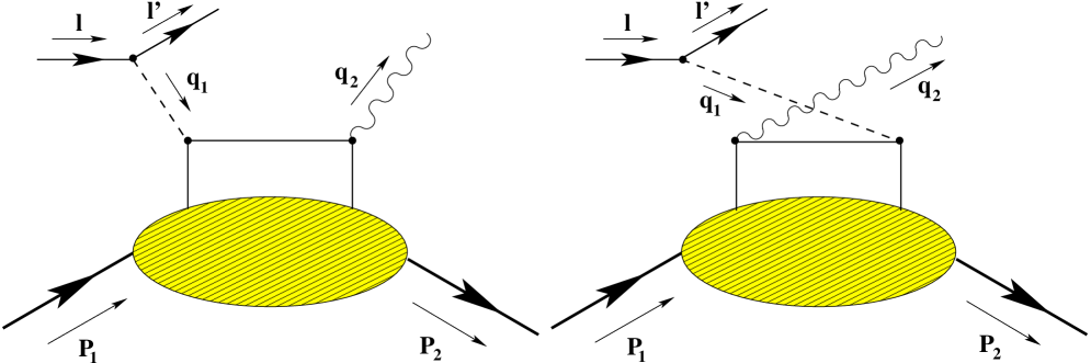
Figure 5.1: Leading hand-bag diagrams for the process

$$P_{1,2}=\bar{P}\pm\frac{\Delta}{2}\,\,\,\,\,\,\,\,q_{1,2}=\bar{q}\mp\frac{\Delta}{2}$$ (5.1)

with $-\Delta=P_{2}-P_{1}$ being the momentum transfer. Clearly

$$\bar{P}\cdot\Delta=0,\,\,\,\,\,t=\Delta^{2}\,\,\,\,\,\,\,\bar{P}^{2}=M^{2}-\frac{t}{4}$$ (5.2)

and $M$ is the nucleon mass. There are two scaling variables which are identified in the process, since 3 scalar products can grow large in the generalized Bjorken limit: $\bar{q}^{2}$, $\Delta\cdot q$, $\bar{P}\cdot\bar{q}$.

The momentum transfer $t=\Delta^{2}$ is a small parameter in the process. Momentum asymmetries between the initial and the final state nucleon are measured by two scaling parameters, $\xi$ and $\eta$, related to ratios of the former invariants

$$\xi=-{\bar{q}^{2}\over 2\bar{P}\cdot{\bar{q}}}\,\,\,\,\,\,\,\,\,\,\,\,\eta={\Delta\cdot\bar{q}\over 2\bar{P}\cdot\bar{q}}$$ (5.3)

where $\xi$ is a variable of Bjorken type, expressed in terms of average momenta rather than nucleon and Z-boson momenta. The standard Bjorken variable $x=-q_{1}^{2}/(2P_{1}\cdot q_{1})$ is trivially related to $\xi$ in the $t=0$ limit. In the DIS limit $(P_{1}=P_{2})$ $\eta=0$ and $x=\xi$, while in the DVCS limit $\eta=\xi$ and $x=2\xi/(1+\xi)$, as one can easily deduce from the relations

$$q_{1}^{2}=\left(1+\frac{\eta}{\xi}\right)\bar{q}^{2}+\frac{t}{4},\,\,\,\,\,\,\,\,\,\,q_{2}^{2}=\left(1-\frac{\eta}{\xi}\right)\bar{q}^{2}+\frac{t}{4}.$$ (5.4)

We introduce also the inelasticity parameter $y=P_{1}\cdot l/(P_{1}\cdot q_{1})$ which measures the fraction of the total energy that is transferred to the final state photon. Notice also that $\xi=\frac{\Delta^{+}}{2\bar{P}^{+}}$ measures the ratio between the plus component of the momentum transfer and the average momentum. A second scaling variable, related to $\xi$ is $\zeta={\Delta^{+}}/{{P_{1}}^{+}}$, which coincides with Bjorken $x$ $(x=\zeta)$ when $t=0$. $\xi$, therefore, parametrizes the large component of the momentum transfer $\Delta$, which can be generically described as

$$\Delta=2\xi\bar{P}+\hat{\Delta}$$ (5.5)

where all the components of $\hat{\Delta}$ are $O(\sqrt{t})$ [104].

5.3 DIS versus DVNS

In the study of ordinary DIS scattering of neutrinos on nucleons (see Fig. 5.2), the relevant current correlator is obtained from the T-product of two neutral currents acting on a forward nucleon state of momentum $P_{1}$

$$j_{Z}^{\mu} \equiv \overline{u}(l^{\prime})\gamma^{\mu}\left(-1+4\sin^{2}\theta_{W}+\gamma_{5}\right)u(l)$$ (5.6)

where $\theta_{W}$ is the Weinberg angle, $l$ and $l^{\prime}$ are the initial and final-state lepton. The relevant correlator is given by

$$T_{\mu\nu}(q_{1}^{2},\nu)=i\int d^{4}ze^{iq\cdot z}\langle P_{1}|T(J_{Z}^{\mu}(\xi)J_{Z}^{\nu}(0)|P_{1}\rangle$$ (5.7)

with $\nu=E-E^{\prime}$ being the energy transfered to the nucleon, $P_{1}$ is the initial-state nucleon 4-momenta and $q_{1}=l-l^{\prime}$ is the momentum transfered. The hadronic tensor $W_{\mu\nu}$ is related to the imaginary part of this correlator by the optical theorem. We recall that for an inclusive electroweak process mediated by neutral currents the hadronic tensor (for unpolarized scatterings) is identified in terms of 3 independent structure functions at leading twist

$$W_{\mu\nu}=\left(-g_{\mu\nu}+{q_{1\mu}q_{1\nu}\over q_{1}^{2}}\right)W_{1}(\nu,Q^{2})+{\hat{P_{1}}^{\mu}\hat{P_{1}}^{\nu}\over P_{1}^{2}}{W_{2}(\nu,Q^{2})\over M^{2}}-i\epsilon_{\mu\nu\lambda\sigma}{q_{1}^{\lambda}P_{1}^{\sigma}}{W_{3}(\nu,Q^{2})\over 2M^{2}}$$ (5.8)

where transversality of the current is obvious since $\hat{P_{1}}^{\mu}=P_{1}^{\mu}-q_{1}^{\mu}{P_{1}\cdot q_{1}}/{q_{1}^{2}}$.

The analysis at higher twists is far more involved and the total number of structure functions appearing is 14 if we include polarization effects. These are fixed by the requirements of Lorenz covariance and time reversal invariance, neglecting small CP-violating effects from the CKM matrix. Their number can be reduced to 8 if current conservation is imposed, which is equivalent to requiring that contributions proportional to non-vanishing current quark masses can be dropped (see also [128]). We recall that the DIS limit is performed by the identifications

$$MW_{1}(Q^{2},\nu) = F_{1}(x,Q^{2})$$

$$\nu W_{2}(Q^{2},\nu) = F_{2}(x,Q^{2})$$

$$\nu W_{3}(Q^{2},\nu) = F_{3}(x,Q^{2}),$$ (5.9)

in terms of the standard structure functions $F_{1}$, $F_{2}$ and $F_{3}$. There are various ways to express the neutrino-nucleon DIS cross section, either in terms of $Q^{2}$ and the energy transfer, in which the scattering angle $\theta$ is integrated over, or as a triple cross section in $(Q^{2},\nu,\theta)$, or yet in terms of the Bjorken variable $x$, inelasticity $y$ and the scattering angle $(x,y,\theta)$. This last case is close to the kinematical setup of our study. In this case the differential Born cross section in DIS is given by

$$\frac{d^{3}\sigma}{dxdyd\theta}=\frac{y\alpha^{2}}{Q^{4}}\sum_{i}\eta_{i}(Q^{2})L_{i}^{\mu\nu}W_{i}^{\mu\nu},$$ (5.10)

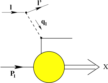
Figure 5.2: Leading diagram for a generic DIS process

the index $i$ denotes the different current contributions, ( $i=|\gamma|^{2},|\gamma Z|,|Z|^{2}$ for the neutral current) and $\alpha$ denotes the fine structure constant. By $\theta$ we indicate the azimuthal angle of the final-state lepton, while $y=(P_{1}\cdot q_{1})/(l\cdot P_{1})$ is the inelasticity parameter, and $Q^{2}=-q_{1}^{2}$. The factors $\eta_{i}(Q^{2})$ denote the ratios of the corresponding propagator terms to the photon propagator squared,

$$\eta^{|\gamma|^{2}}(Q^{2}) = 1,$$

$$\eta^{|\gamma Z|}(Q^{2}) = \frac{G_{F}M_{Z}^{2}}{2\sqrt{2}\pi\alpha}\frac{Q^{2}}{Q^{2}+M_{Z}^{2}},$$

$$\eta^{|Z|^{2}}(Q^{2}) = (\eta^{|\gamma Z|})^{2}(Q^{2}).$$

where $G_{F}$ is the Fermi constant and $M_{Z}$ is the mass of the $Z$ boson while the leptonic tensor has the form

$$L_{\mu\nu}^{i}=\sum_{\lambda^{\prime}}\left[\bar{u}(k^{\prime},\lambda^{\prime})\gamma_{\mu}(g_{V}^{i_{1}}+g_{A}^{i_{1}}\gamma_{5})u(k,\lambda)\right]^{\ast}\bar{u}(k^{\prime},\lambda^{\prime})\gamma_{\nu}(g_{V}^{i_{2}}+g_{A}^{i_{2}}\gamma_{5})u(k,\lambda).$$ (5.12)

In the expression above $\lambda$ and $\lambda^{\prime}$, denote the initial and final-state helicity of the leptons. The indices $i_{1}$ and $i_{2}$ refer to the sum appearing in eq. (5.10)

$$\begin{array}[]{lcllcl}g_{V}^{\gamma}&=&1,&g_{A}^{\gamma}&=&0,\\ g_{V}^{Z}&=&-\frac{1}{2}+2\sin^{2}\theta_{W},&g_{A}^{Z}&=&\frac{1}{2},\\ \end{array}$$ (5.13)

In the case of neutrino/nucleon interaction mediated by the neutral current the dominant diagram for this process appears in Fig. 5.2. A similar diagram, with the obvious modifications, describes also charged current exchanges. We recall that the unpolarized cross section is expressed in terms of $F_{1}$ and $F_{2}$, since $F_{3}$ disappears in this special case, and in particular, after an integration over the scattering angle of the final state neutrino one obtains

$$\frac{d^{2}\sigma}{dxdy}=2\pi S{\alpha^{2}\over Q^{4}}(g_{V}^{Z})^{2}\eta^{|\gamma Z|}(Q^{2})\left(2xy^{2}F_{1}+2(1-x-{xyM^{2}\over S})F_{2}\right).$$ (5.14)

where $S=2ME_{\nu}$ is the nucleon-neutrino center of mass energy.

We also recall that in this case the cross section in the parton model is given by

$$\frac{d^{2}\sigma}{dxdy}=\frac{G_{F}^{2}ME_{\nu}}{2\pi}\left(\frac{M_{Z}^{2}}{Q^{2}+M_{Z}^{2}}\right)^{2}\left[xq^{0}(x,Q^{2})+x\bar{q}^{0}(x,Q^{2})(1-y)^{2}\right]$$ (5.15)

where $q^{0}(x,Q^{2})$ and $\bar{q}^{0}(x,Q^{2})$ are linear combinations of parton distributions

$$q^{0}(x,Q^{2}) = \left[\frac{u_{v}(x,Q^{2})+d_{v}(x,Q^{2})}{2}+\frac{\bar{u}(x,Q^{2})+\bar{d}(x,Q^{2})}{2}\right]\left(L_{u}^{2}+L_{d}^{2}\right)$$

$$+ \left[\frac{\bar{u}(x,Q^{2})+\bar{d}(x,Q^{2})}{2}\right]\left(R_{u}^{2}+R_{d}^{2}\right)$$

$$\bar{q}^{0}(x,Q^{2}) = \left[\frac{u_{v}(x,Q^{2})+d_{v}(x,Q^{2})}{2}+\frac{\bar{u}(x,Q^{2})+\bar{d}(x,Q^{2})}{2}\right]\left(R_{u}^{2}+R_{d}^{2}\right)$$

$$+ \left[\frac{\bar{u}(x,Q^{2})+\bar{d}(x,Q^{2})}{2}\right]\left(L_{u}^{2}+L_{d}^{2}\right)$$

with

$$L_{u}=1-\frac{4}{3}\sin^{2}\theta_{W}\,,\hskip 42.67912ptL_{d}=-1+\frac{2}{3}\sin^{2}\theta_{W}$$

$$R_{u}=-\frac{4}{3}\sin^{2}\theta_{W}\,,\hskip 51.21504ptR_{d}=\frac{2}{3}\sin^{2}\theta_{W}$$

and we have identified the sea contributions $u_{s}$ and $d_{s}$ with $\bar{u}$ and $\bar{d}$ rispectively.

Figure 5.3: The cross section of a neutrino process of DIS-type at $x\approx 0.1$ with neutral current at ultrahigh energy

Let’s now move to the nonforward case. Here, when a real photon is present in the final state, the relevant correlator is given by

$$T_{\mu\nu}(q_{1}^{2},\nu)=i\int d^{4}ze^{iq\cdot z}\langle\bar{P}-{\Delta\over 2}|T(J_{Z}^{\mu}(-z/2)J_{\gamma}^{\nu}(z/2)|\bar{P}+{\Delta\over 2}\rangle.$$ (5.18)

The dominant diagrams for this process appears in Fig 5.1. We impose Ward identities on both indices, which is equivalent to requiring that terms proportional to the quark masses in $\partial\cdot J_{Z}$ are neglected. This approximation is analogous to the one performed in the forward case in order to reduce the structure functions from 8 to 3 (in the absence of any polarization), imposing symmetric trasversality conditions on the weak currents

$$\left(\bar{P}^{\mu}-{\Delta^{\mu}\over 2}\right)T_{\mu\nu}=0\,\,\,\,\,\,\,\,\,\left(\bar{P}^{\mu}+{\Delta^{\mu}\over 2}\right)T_{\mu\nu}=0.$$ (5.19)

The leading twist contribution to DVNS is obtained by performing a collinear expansion of the loop momentum of the hand-bag diagram and neglecting terms of order $O(\Delta_{\perp}^{2}/Q^{2})$ and $M^{2}/Q^{2}$. Transversality is satisfied at this order. Violation of transversality condition in the hand-bag approximation is analogous to the DVCS case, where it has been pointed out that one has to include systematically “kinematical” twist-3 operators, which appear as total derivatives of twist-2 operators [104] [105] in order to restore it.

For the parametrization of the hand-bag diagram (Fig. 5.1) we use the light-cone decomposition in terms of 2 four-vectors $(n,\tilde{n})$, where

$$\tilde{n}^{\mu} = \Lambda(1,0,0,1)$$

$$n^{\mu} = \frac{1}{2\Lambda}(1,0,0,-1)$$

$$\tilde{n}^{2} = n^{2}=0\ \ \ ,\ \ \ \tilde{n}\cdot n=1.$$

At the same time we set

$$P_{1}^{\mu} = (1+\xi)\tilde{n}^{\mu}+(1-\xi){\overline{M}\over 2}n^{\mu}-{\Delta_{\perp}^{\mu}\over 2}$$

$$P_{2}^{\mu} = (1+\xi)\tilde{n}^{\mu}+(1+\xi){\overline{M}\over 2}n^{\mu}+{\Delta_{\perp}^{\mu}\over 2}$$

$$q_{1}^{\mu} = -2\xi\tilde{n}^{\mu}+{Q^{2}\over 4\xi}n^{\mu}$$

$$k^{\mu} = \left(k\cdot n\,\right)\,\tilde{n}^{\mu}+\left(k\cdot\tilde{n}\right)\,\,n^{\mu}+k_{\perp}^{\mu}$$

$$\overline{M}^{2} = M^{2}-\frac{\Delta^{2}}{4}$$ (5.20)

with $\bar{P}^{2}=\overline{M}^{2}$. We will also use the notation $-q_{1}^{2}=Q^{2}$ for the invariant mass of the virtual $Z$ boson and we will denote by $\bar{q}$ the average gauge bosons momenta respectively.

After a collinear expansion of the loop momentum we obtain

$$T_{A}^{\mu\nu}=i\int\frac{d^{4}k}{(2\pi)^{4}}Tr\left\{g_{u}\gamma^{\nu}\hbox to0.0pt{/\hss}{P_{D}}\gamma^{\mu}\tilde{g}\left(U_{v}-\gamma^{5}\right)\underline{M}^{u}(k)+\right.$$

$$\hskip 99.58464pt\left.g_{d}\gamma^{\nu}\hbox to0.0pt{/\hss}{P_{D}}\gamma^{\mu}\tilde{g}\left(D_{v}-\gamma^{5}\right)\underline{M}^{d}(k)\right\}$$

$$T_{B}^{\mu\nu}=i\int\frac{d^{4}k}{(2\pi)^{4}}Tr\left\{\tilde{g}\gamma^{\mu}\left(U_{v}-\gamma^{5}\right)\hbox to0.0pt{/\hss}{P_{E}}\gamma^{\nu}g_{u}\underline{M}^{u}(k)+\right.$$

$$\hskip 99.58464pt\left.\tilde{g}\gamma^{\mu}\left(D_{v}-\gamma^{5}\right)\hbox to0.0pt{/\hss}{P_{E}}\gamma^{\nu}g_{d}\underline{M}^{d}(k)\right\}$$ (5.21)

where we have used the following notations

$$g_{u}=\frac{2}{3}e,\hskip 28.45274ptg_{d}=\frac{1}{3}e,\hskip 28.45274pt\tilde{g}=\frac{g}{4\cos{(\theta_{W})}},$$

$$U_{v}=1-\frac{8}{3}\sin^{2}\theta_{W},\hskip 28.45274ptD_{v}=1-\frac{4}{3}\sin^{2}\theta_{W},$$

(5.22)

$$\hbox to0.0pt{/\hss}{P_{D}}=\frac{k\hskip-6.0pt/\hskip 6.0pt-\alpha\Delta\hskip-6.0pt/\hskip 6.0pt+q_{1}\hskip-6.0pt/\hskip 6.0pt}{\left(k-\alpha\Delta+q_{1}\right)^{2}+i\epsilon}\,\,,$$

$$\hbox to0.0pt{/\hss}{P_{E}}=\frac{k\hskip-6.0pt/\hskip 6.0pt-q_{1}\hskip-6.0pt/\hskip 6.0pt+\Delta\hskip-6.0pt/\hskip 6.0pt(1-\alpha)}{\left(k-q_{1}+\Delta(1-\alpha)\right)^{2}+i\epsilon}\,\,$$ (5.23)

where the constant $\alpha$ ($\alpha$ is a free parameter) ranges between $0$ and $1$. The $\underline{M}$ matrix is the quark density matrix and is given by

$$\underline{M}_{ab}^{(i)}(k) = \int d^{4}ye^{ik\cdot y}\langle P^{\prime}|\overline{\psi}_{a}^{(i)}(-\alpha y)\psi_{b}^{(i)}((1-\alpha)y)|P\rangle.$$ (5.24)

The index $i=u,d$ runs on flavours. Using a Sudakov decomposition of the internal loop we can rewrite $T_{A}^{\mu\nu}$ and $T_{B}^{\mu\nu}$ as

$$T_{A}^{\mu\nu}=i\,\int\frac{d(k\cdot n)}{(2\pi)^{4}}d(k\cdot\tilde{n})d^{2}k_{\perp}\int\frac{d\lambda}{(2\pi)}dze^{i\lambda(z-k\cdot n)}$$

$$\;\;\;\;\;\;\;\;\;\;\;\;Tr\left\{g_{u}\gamma^{\nu}\hbox to0.0pt{/\hss}{P_{D}}\gamma^{\mu}\tilde{g}\left(U_{v}-\gamma^{5}\right)\underline{M}^{u}(k)+\right.$$

$$\hskip 56.9055pt\left.g_{d}\gamma^{\nu}\hbox to0.0pt{/\hss}{P_{D}}\gamma^{\mu}\tilde{g}\left(D_{v}-\gamma^{5}\right)\underline{M}^{d}(k)\right\}$$

(5.25)

$$T_{B}^{\mu\nu}=i\,\int\frac{d(k\cdot n)}{(2\pi)^{4}}d(k\cdot\tilde{n})d^{2}k_{\perp}\int\frac{d\lambda}{(2\pi)}dze^{i\lambda(z-k\cdot n)}$$

$$\;\;\;\;\;\;\;\;\;\;\;\;Tr\left\{\tilde{g}\gamma^{\mu}\left(U_{v}-\gamma^{5}\right)\hbox to0.0pt{/\hss}{P_{E}}\gamma^{\nu}g_{u}\underline{M}^{u}(k)+\right.$$

$$\hskip 56.9055pt\left.\tilde{g}\gamma^{\mu}\left(D_{v}-\gamma^{5}\right)\hbox to0.0pt{/\hss}{P_{E}}\gamma^{\nu}g_{d}\underline{M}^{d}(k)\right\}$$ (5.26)

to which we will refer as the direct and the exchange diagram respectively. It is also convenient to introduce two new linear combinations $T^{\mu\nu}=T_{A}^{\mu\nu}+T_{B}^{\mu\nu}=\tilde{T}_{A}^{\mu\nu}+\tilde{T}_{B}^{\mu\nu}$ which will turn useful in order to separate Vector (V) and axial vector parts (A) of the expansion

$$\tilde{T}_{A}^{\mu\nu}=i\int\frac{d(k\cdot n)}{(2\pi)^{4}}d(k\cdot\tilde{n})d^{2}k_{\perp}\int\frac{d\lambda}{(2\pi)}dze^{i\lambda(z-k\cdot n)}$$

$$\;\;\;\;\;\;\;\;\;\;\;\;\tilde{g}g_{u}U_{v}Tr\left\{\left[\gamma^{\nu}\hbox to0.0pt{/\hss}{P_{D}}\gamma^{\mu}+\gamma^{\mu}\hbox to0.0pt{/\hss}{P_{E}}\gamma^{\nu}\right]\underline{M}^{u}(k)\right\}+$$

$$\hskip 39.83368pt\tilde{g}g_{d}D_{v}Tr\left\{\left[\gamma^{\nu}\hbox to0.0pt{/\hss}{P_{D}}\gamma^{\mu}+\gamma^{\mu}\hbox to0.0pt{/\hss}{P_{E}}\gamma^{\nu}\right]\underline{M}^{d}(k)\right\}$$

(5.27)

$$\tilde{T}_{B}^{\mu\nu}=-i\int\frac{d(k\cdot n)}{(2\pi)^{4}}d(k\cdot\tilde{n})d^{2}k_{\perp}\int\frac{d\lambda}{(2\pi)}dze^{i\lambda(z-k\cdot n)}$$

$$\;\;\;\;\;\;\;\;\;\;\;\;\tilde{g}g_{u}Tr\left\{\left[\gamma^{\nu}\hbox to0.0pt{/\hss}{P_{D}}\gamma^{\mu}+\gamma^{\mu}\hbox to0.0pt{/\hss}{P_{E}}\gamma^{\nu}\right]\gamma^{5}\underline{M}^{u}(k)\right\}+$$

$$\hskip 39.83368pt\tilde{g}g_{d}Tr\left\{\left[\gamma^{\nu}\hbox to0.0pt{/\hss}{P_{D}}\gamma^{\mu}+\gamma^{\mu}\hbox to0.0pt{/\hss}{P_{E}}\gamma^{\nu}\right]\gamma^{5}\underline{M}^{d}(k)\right\}.$$ (5.28)

with $\tilde{T}_{A}$ including the vector parts $(V\times V\,\,+\,\,A\times A)$ and $\tilde{T}_{B}$ the axial-vector parts

$(V\times A\,\,+\,\,A\times V)$. After some algebraic manipulations we finally obtain

$$\tilde{T}_{A}^{\mu\nu}=\frac{i}{2}\sum_{i=u,d}\tilde{g}g_{i}C_{i}\int\frac{d\lambda dz}{(2\pi)}e^{i\lambda z}\left\{\left(\tilde{n}^{\mu}n^{\nu}+\tilde{n}^{\nu}n^{\mu}-g^{\mu\nu}\right)\alpha(z)\langle P^{\prime}|\overline{\psi}^{(i)}\left(-\frac{\lambda n}{2}\right)n\hskip-6.0pt/\hskip 6.0pt\psi^{(i)}\left(\frac{\lambda n}{2}\right)|P\rangle\right.$$

$$\hskip 142.26378pt\left.+i\epsilon^{\mu\nu\alpha\beta}\tilde{n}_{\alpha}n_{\beta}\beta(z)\langle P^{\prime}|\overline{\psi}^{(i)}\left(-\frac{\lambda n}{2}\right)\gamma^{5}n\hskip-6.0pt/\hskip 6.0pt\psi^{(i)}\left(\frac{\lambda n}{2}\right)|P\rangle\right\}$$

$$\tilde{T}_{B}^{\mu\nu}=-\frac{i}{2}\sum_{i=u,d}\tilde{g}g_{i}\int\frac{d\lambda dz}{(2\pi)}e^{i\lambda z}\left\{\left(\tilde{n}^{\mu}n^{\nu}+\tilde{n}^{\nu}n^{\mu}-g^{\mu\nu}\right)\alpha(z)\langle P^{\prime}|\overline{\psi}^{(i)}\left(-\frac{\lambda n}{2}\right)\gamma^{5}n\hskip-6.0pt/\hskip 6.0pt\psi^{(i)}\left(\frac{\lambda n}{2}\right)|P\rangle\right.$$

$$\hskip 142.26378pt\left.+i\epsilon^{\mu\nu\alpha\beta}\tilde{n}_{\alpha}n_{\beta}\beta(z)\langle P^{\prime}|\overline{\psi}^{(i)}\left(-\frac{\lambda n}{2}\right)n\hskip-6.0pt/\hskip 6.0pt\psi^{(i)}\left(\frac{\lambda n}{2}\right)|P\rangle\right\}$$

where $C_{i}=U_{v},\,D_{v}$ and

$$\alpha(z)=\left(\frac{1}{z-{\xi}+i\epsilon}+\frac{1}{z+{\xi}-i\epsilon}\right),\hskip 42.67912pt\beta(z)=\left(\frac{1}{z-{\xi}+i\epsilon}-\frac{1}{z+{\xi}-i\epsilon}\right)$$ (5.30)

are the “first order” propagators appearing in the factorization of the amplitude. We recall, if not obvious, that differently from DIS, DVCS undergoes factorization directly at amplitude level [106].

The parameterizations of the non-forward light cone correlators in terms of GPD’s is of the form given by Ji at leading twist [100]

$$\int\frac{d\lambda}{(2\pi)}e^{i\lambda z}\langle P^{\prime}|\overline{\psi}\left(-\frac{\lambda n}{2}\right)\gamma^{\mu}\psi\left(\frac{\lambda n}{2}\right)|P\rangle=$$

$$H(z,\xi,\Delta^{2})\overline{U}(P^{\prime})\gamma^{\mu}U(P)+E(z,\xi,\Delta^{2})\overline{U}(P^{\prime})\frac{i\sigma^{\mu\nu}\Delta_{\nu}}{2M}U(P)+.....$$

$$\int\frac{d\lambda}{(2\pi)}e^{i\lambda z}\langle P^{\prime}|\overline{\psi}\left(-\frac{\lambda n}{2}\right)\gamma^{\mu}\gamma^{5}\psi\left(\frac{\lambda n}{2}\right)|P\rangle=$$

$$\tilde{H}(z,\xi,\Delta^{2})\overline{U}(P^{\prime})\gamma^{\mu}\gamma^{5}U(P)+\tilde{E}(z,\xi,\Delta^{2})\overline{U}(P^{\prime})\frac{\gamma^{5}\Delta^{\mu}}{2M}U(P)+.....$$ (5.31)

which have been expanded in terms of functions $H,E,\tilde{H},\tilde{E}$ [127] and the ellipses are meant to denote the higher-twist contributions. It is interesting to observe that the amplitude is still described by the same light-cone correlators as in the electromagnetic case (vector, axial vector) but now parity is not conserved.

5.4 Operatorial analysis

The operatorial structure of the T-order product of one electroweak current and one electromagnetic current is relevant in order to identify the independent amplitudes appearing in the correlator at leading twist and the study is presented here. We will identify four operatorial structures. For this purpose let’s start from the Fourier transform of the correlator of the two currents

$$T_{\mu\nu}=i\int d^{4}xe^{iqx}\langle P_{2}|T\left(J_{\nu}^{\gamma}(x/2)J_{\mu}^{Z_{0}}(-x/2)\right)|P_{1}\rangle\,,$$ (5.32)

where for the neutral and electromagnetic currents we have the following expressions

$$J^{\mu Z_{0}}(-x/2)=\frac{g}{2\cos{\theta_{W}}}\overline{\psi}_{u}(-x/2)\gamma^{\mu}(g^{Z}_{uV}+g^{Z}_{uA}\gamma^{5})\psi_{u}(-x/2)+\overline{\psi}_{d}(-x/2)\gamma^{\mu}(g^{Z}_{dV}+g^{Z}_{dA}\gamma^{5})\psi_{d}(-x/2),\,$$

$$J^{\nu,\gamma}(x/2)=\overline{\psi}_{d}(x/2)\gamma^{\nu}\left(-\frac{1}{3}e\right)\psi_{d}(x/2)+\overline{\psi}_{u}(x/2)\gamma^{\nu}\left(\frac{2}{3}e\right)\psi_{u}(x/2)\,.$$ (5.33)

By simple calculations one obtains

$$\langle P_{2}|T\left(J_{\nu}^{\gamma}(x/2)J_{\mu}^{Z_{0}}(-x/2)\right)|P_{1}\rangle=$$

$$\langle P_{2}|\overline{\psi}_{u}(x/2)g_{u}\gamma_{\nu}S(x)\gamma_{\mu}(g^{Z}_{uV}+g^{Z}_{uA}\gamma^{5})\psi_{u}(-x/2)-$$

$$\hskip 22.76228pt\overline{\psi}_{d}(x/2)g_{d}\gamma_{\nu}S(x)\gamma_{\mu}(g^{Z}_{dV}+g^{Z}_{dA}\gamma^{5})\psi_{d}(-x/2)+$$

$$\hskip 22.76228pt\overline{\psi}_{u}(x/2)\gamma_{\mu}(g^{Z}_{uV}+g^{Z}_{uA}\gamma^{5})S(-x)g_{u}\gamma_{\nu}\psi_{u}(x/2)-$$

$$\hskip 22.76228pt\overline{\psi}_{d}(x/2)\gamma_{\mu}(g^{Z}_{dV}+g^{Z}_{dA}\gamma^{5})S(-x)g_{d}\gamma_{\nu}\psi_{d}(x/2)|P_{1}\rangle\,.$$

The coefficients used in eqs. (5.4, 5.4) $g_{V}^{Z}$ and $g_{A}^{Z}$, are

$$g^{Z}_{uV}=\frac{1}{2}+\frac{4}{3}\sin^{2}\theta_{W}\hskip 42.67912ptg^{Z}_{uA}=-\frac{1}{2}$$

$$g^{Z}_{dV}=-\frac{1}{2}+\frac{2}{3}\sin^{2}\theta_{W}\hskip 42.67912ptg^{Z}_{dA}=\frac{1}{2}\,,$$ (5.35)

and

$$g_{u}=\frac{2}{3}, g_{d}=\frac{1}{3}$$ (5.36)

are the absolute values of the charges of the up and down quarks in units of the electron charge.

The function $S(x)$ denotes the free quark propagator

$$S(x)\approx\frac{i\hbox to0.0pt{/\hss}{x}}{2\pi^{2}(x^{2}-i\epsilon)^{2}}.$$ (5.37)

After some standard identities for the $\gamma$’s products

$$\gamma_{\mu}\gamma_{\alpha}\gamma_{\nu}=S_{\mu\alpha\nu\beta}\gamma^{\beta}+i\epsilon_{\mu\alpha\nu\beta}\gamma^{5}\gamma^{\beta},$$

$$\gamma_{\mu}\gamma_{\alpha}\gamma_{\nu}\gamma^{5}=S_{\mu\alpha\nu\beta}\gamma^{\beta}\gamma^{5}-i\epsilon_{\mu\alpha\nu\beta}\gamma^{\beta},$$

$$S_{\mu\alpha\nu\beta}=\left(g_{\mu\alpha}g_{\nu\beta}+g_{\nu\alpha}g_{\mu\beta}-g_{\mu\nu}g_{\alpha\beta}\right),$$ (5.38)

we rewrite the correlators as

$$T_{\mu\nu}=i\int d^{4}x\frac{e^{iqx}x^{\alpha}}{2\pi^{2}(x^{2}-i\epsilon)^{2}}\langle P_{2}|\left[g_{u}g_{uV}\left(S_{\mu\alpha\nu\beta}O^{\beta}_{u}-i\epsilon_{\mu\alpha\nu\beta}O^{5\beta}_{u}\right)-g_{u}g_{uA}\left(S_{\mu\alpha\nu\beta}\tilde{O}^{5\beta}_{u}-i\epsilon_{\mu\alpha\nu\beta}\tilde{O}^{\beta}_{u}\right)\right.$$

$$\hskip 156.49014pt\left.-g_{d}g_{dV}\left(S_{\mu\alpha\nu\beta}O^{\beta}_{d}-i\epsilon_{\mu\alpha\nu\beta}O^{5\beta}_{d}\right)+g_{d}g_{dA}\left(S_{\mu\alpha\nu\beta}\tilde{O}^{5\beta}_{d}-i\epsilon_{\mu\alpha\nu\beta}\tilde{O}^{\beta}_{d}\right)\right]|P_{1}\rangle.\,$$

The $x$-dependence of the operators in the former equations was suppressed.

Whence the relevant operators are denoted by

$$\tilde{O}_{a}^{\beta}(x/2,-x/2)=\overline{\psi}_{a}(x/2)\gamma^{\beta}\psi_{a}(-x/2)+\overline{\psi}_{a}(-x/2)\gamma^{\beta}\psi_{a}(x/2),$$

$$\tilde{O}_{a}^{5\beta}(x/2,-x/2)=\overline{\psi}_{a}(x/2)\gamma^{5}\gamma^{\beta}\psi_{a}(-x/2)-\overline{\psi}_{a}(-x/2)\gamma^{5}\gamma^{\beta}\psi_{a}(x/2),$$

$$O_{a}^{\beta}(x/2,-x/2)=\overline{\psi}_{a}(x/2)\gamma^{\beta}\psi_{a}(-x/2)-\overline{\psi}_{a}(-x/2)\gamma^{\beta}\psi_{a}(x/2),$$

$$O_{a}^{5\beta}(x/2,-x/2)=\overline{\psi}_{a}(x/2)\gamma^{5}\gamma^{\beta}\psi_{a}(-x/2)+\overline{\psi}_{a}(-x/2)\gamma^{5}\gamma^{\beta}\psi_{a}(x/2)\,,$$

where $a$ is a flavour index.

5.5 Phases of the Amplitude

The numerical computation of the cross section requires a prescription for a correct handling of the singularities in the integration region at $z=\pm\xi$. The best way to proceed is to work out explicitly the structure of the factorization formula of the amplitude using the Feynman prescription for going around the singularities, thereby isolating a principal value integral (P.V., which is real) and an imaginary contribution coming from the $\delta$ function term. A P.V. integral is expressed in terms of “plus” distributions and of logarithmic terms, as illustrated below. The expression of the factorization formula of the process in the parton model, in which $\alpha(z)$ and $\beta(z)$ appear as factors in the coefficient functions, is then given by

$$\hskip 113.81102pt{\cal{M}}_{fi}=J^{\mu}_{Z}(q_{1})D(q_{1})\epsilon^{\nu*}(q_{1}-\Delta)$$

$$\times\left\{\frac{i}{2}\tilde{g}g_{u}U_{v}\int_{-1}^{1}dz\left(\tilde{n}^{\mu}n^{\nu}+\tilde{n}^{\nu}n^{\mu}-g^{\mu\nu}\right)\right.$$

$$\left.\alpha(z)\left[H^{u}(z,\xi,\Delta^{2})\overline{U}(P_{2})n\hskip-6.0pt/\hskip 6.0ptU(P_{1})+E^{u}(z,\xi,\Delta^{2})\overline{U}(P_{2})\frac{i\sigma^{\mu\nu}n_{\mu}\Delta_{\nu}}{2M}U(P_{1})\right]+\right.$$

$$\left.\beta(z)i\epsilon^{\mu\nu\alpha\beta}\tilde{n}_{\alpha}n_{\beta}\left[\tilde{H}^{u}(z,\xi,\Delta^{2})\overline{U}(P_{2})n\hskip-6.0pt/\hskip 6.0pt\gamma^{5}U(P_{1})+\tilde{E}^{u}(z,\xi,\Delta^{2})\overline{U}(P_{2})\gamma^{5}\left(\Delta\cdot n\right)U(P_{1})\right]+\right.$$

$$\left.\frac{i}{2}\tilde{g}g_{d}D_{v}\int_{-1}^{1}dz\left\{u\rightarrow d\right\}-\right.$$

$$\left.\frac{i}{2}\tilde{g}g_{u}\int_{-1}^{1}dz\left(-\tilde{n}^{\mu}n^{\nu}-\tilde{n}^{\nu}n^{\mu}+g^{\mu\nu}\right)\right.$$

$$\left.\alpha(z)\left[\tilde{H}^{u}(z,\xi,\Delta^{2})\overline{U}(P_{2})n\hskip-6.0pt/\hskip 6.0pt\gamma^{5}U(P_{1})+\tilde{E}^{u}(z,\xi,\Delta^{2})\overline{U}(P_{2})\frac{i\gamma^{5}\Delta\cdot n}{2M}U(P_{1})\right]+\right.$$

$$\left.\beta(z)i\epsilon^{\mu\nu\alpha\beta}\tilde{n}_{\alpha}n_{\beta}\left[H^{u}(z,\xi,\Delta^{2})\overline{U}(P_{2})n\hskip-6.0pt/\hskip 6.0ptU(P_{1})+E^{u}(z,\xi,\Delta^{2})\overline{U}(P_{2})\frac{i\sigma^{\mu\nu}n_{\mu}\Delta_{\nu}}{2M}(P_{1})\right]-\right.$$

$$\left.\frac{i}{2}\tilde{g}g_{d}\int_{-1}^{1}dz\left\{u\rightarrow d\right\}\right\}.$$

To handle the singularity on the path of integration in the factorization formula, as we have already mentioned, we use the Feynman ($i\epsilon$) prescription, thereby generating imaginary parts. In particular, any standard integral containing imaginary parts is then separated into real and imaginary contributions as

$$\int dz{T(z)\over z\mp\xi\pm i\epsilon}=PV\int_{-1}^{1}dz{T(z)\over z\mp\xi}\,\mp\,i\pi T(\pm\xi)$$ (5.42)

for a real coefficient $T(z)$. We then rewrite the P.V. integral in terms of “plus” distributions

$$P.V.\int_{-1}^{1}dz{H(z)\over z-\xi} = \int_{-1}^{1}dz\frac{H(z)-H(\xi)}{z-\xi}+H(\xi)\log\left({1-\xi\over 1+\xi}\right)$$

$$= \int_{-1}^{1}dz{\cal Q}(z)H(z)+\int_{-1}^{1}dz\bar{{\cal Q}}(z)H(z)+H(\xi)\log\left({1-\xi\over 1+\xi}\right)$$

where

$${\cal Q}(z) = \theta(-1\leq z\leq\xi){1\over(z-\xi)_{+}}$$

$$= \theta(-1\leq z\leq\xi)\left({\theta(z<\xi)\over(z-\xi)}-\delta(z-\xi)\int_{-1}^{\xi}{dz\over(z-\xi)}\right)$$

$$\bar{\cal Q}(z) = \theta(\xi\leq z\leq 1){1\over(z-\xi)_{+}}$$

$$= \theta(-1\leq z\leq\xi)\left({\theta(z>\xi)\over(z-\xi)}-\delta(z-\xi)\int_{\xi}^{1}{dz\over(z-\xi)}\right)$$

and the integrals are discretized using finite elements methods, in order to have high numerical accuracy. This last point is illustrated in Appendix C, where the computations are done analytically on a grid and then the grid spacing is sent to zero.

We can now proceed and compute the cross section. We define the scalar amplitude

$${\cal M}_{fi}=J_{Lep}^{\mu}(q_{1})D(q_{1})T^{\mu\nu}\epsilon^{*\nu}(q_{1}-\Delta)$$ (5.45)

where $D(q_{1})$ is the $Z_{0}$ propagator in the Feynman gauge and $J_{Lep}^{\mu}(q_{1})$ is the leptonic current and we have introduced the polarization vector for the final state photon $\epsilon^{\nu}$.

In particular, for the squared amplitude we have

$$|{\cal M}_{fi}|^{2}=-L^{\mu\lambda}D(q_{1})^{2}T_{\mu\nu}T^{*\nu}_{\lambda}\,$$ (5.46)

which is given, more specifically, by

$${\cal|M|}^{2}=\int_{-1}^{1}dz\int_{-1}^{1}dz^{\prime}\left(K_{1}(z,z^{\prime})\alpha(z)\alpha^{*}(z^{\prime})+K_{2}(z,z^{\prime})\beta(z)\beta^{*}(z^{\prime})\right)$$ (5.47)

with $K_{1}$ and $K_{2}$ real functions, combinations of the generalized distributions $(H,\tilde{H},E,\tilde{E})$ with appropriate kinematical factors. Mixed contributions proportional to $\alpha(z)\beta^{*}(z^{\prime})$ and $\beta(z)\alpha^{*}(z^{\prime})$ cancel both in their real and imaginary parts and as such do not contribute to the phases. A similar result holds also for the pure electromagnetic case.

After some further manipulations, we finally rewrite the squared amplitude in terms of a P.V. contribution plus some additional terms coming from the imaginary parts

$${\cal|M|}^{2} = P.V.\int_{-1}^{1}dz\int_{-1}^{1}dz^{\prime}\left(K_{1}(z,z^{\prime})\alpha(z)\alpha^{*}(z^{\prime})+K_{2}(z,z^{\prime})\beta(z)\beta^{*}(z^{\prime})\right)$$ (5.48)

$$+\pi^{2}\left(K_{1}(\xi,\xi)-K_{1}(\xi,-\xi)-K_{1}((-\xi,\xi)+K_{1}(-\xi,-\xi)\right)$$

$$+\pi^{2}\left(K_{2}(\xi,\xi)+K_{2}(\xi,-\xi)+K_{2}((-\xi,\xi)+K_{2}(-\xi,-\xi)\right)$$

which will be analized numerically in the sections below. In order to proceed with the numerical result, it is necessary to review the standard construction of the nonforward parton distribution functions in terms of the forward distributions, which is the topic of the next section.

5.6 Construction of the Input Distributions

The computation of the cross section proceeds rather straightforwardly, though the construction of the initial conditions is more involved compared to the forward (DIS) case. This construction has been worked out in several papers [107, 108, 109, 110, 111, 102, 108] in the case of standard DVCS, using a diagonal input appropriately extended to the non-diagonal kinematics. Different types of nonforward parton distribution, all widely used in the numerical implementations have been put forward, beside Ji’s original distributions, which we will be using in order to construct the initial conditions for our process.

For our purposes it will be useful to introduce Golec-Biernat and Martin’s (GBM) distributions [109] at an intermediate step, which are linearly related to Ji’s distributions.

We recall, at this point, that the quark distributions $H_{q}(z,\xi)$ have support in $z\in[-1,1]$, describing both quark and antiquark distributions for $z>0$ and $z<0$ respectively. In terms of GBM distributions, two distinct distributions ${\hat{\cal{F}}}^{\bar{q}}(X,\zeta)$ and ${\hat{\cal{F}}}^{q}(X,\zeta)$ with $0\leq X\leq 1$ are needed in order to cover the same information contained in Ji’s distributions using only a positive scaling variable ($X$). In the region $X\in(\zeta,1]$ the functions ${\hat{\cal{F}}}^{q}$ and ${\hat{\cal{F}}}^{\bar{q}}$ are independent, but if $X\leq\zeta$ they are related to each other, as shown in the (by now standard) plot in Fig. 5.4.

In this new variable ($X$) the DGLAP region is described by $X>\zeta$ ($|z|>\xi$), and the ERBL region by $X<\zeta$ ($|z|<\xi$). In the ERBL region, $\hat{{\cal F}}^{q}$ and $\hat{{\cal F}}^{\bar{q}}$ are not independent.

The relation between $H(z,\xi)$ and $\hat{{\cal{F}}}^{q}(X,\zeta)$ can be obtained explicitly [112] as follows: for $z\in[-\xi,1]$ we have

$$\hat{{\cal F}}^{q,i}\left(X=\frac{z+\xi}{1+\xi},\zeta\right)=\frac{H^{q,i}(z,\xi)}{1-\zeta/2}\,,$$ (5.49)

and for $z\in[-1,\xi]$

$$\hat{{\cal F}}^{{\bar{q}},i}\left(X=\frac{\xi-z}{1+\xi},\zeta\right)=-\frac{H^{q,i}(z,\xi)}{1-\zeta/2}\,.$$ (5.50)

where $i$ is a flavour index.

Figure 5.4: The relationship between ${\cal F}^{q}(X,\zeta)$, ${\cal F}^{\bar{q}}(X,\zeta)$ and Ji’s function $H^{q}(z,\xi)$.

In our calculations we use a simplified model for the GPD’s where the $\Delta^{2}$ dependence can be factorized as follows [113, 107]

$$H^{i}(z,\xi,\Delta^{2},Q^{2}) = F^{i}_{1}\,(\Delta^{2})q^{i}(z,\xi,Q^{2})$$

$$\tilde{H}^{i}(z,\xi,\Delta^{2},Q^{2}) = G^{i}_{1}(\Delta^{2})\,\Delta{q}^{i}(z,\xi,Q^{2})$$

$$E^{i}(z,\xi,\Delta^{2},Q^{2}) = F^{i}_{2}(\Delta^{2})\,r^{i}(z,\xi,Q^{2})$$ (5.51)

where $q^{i}(z)$ and $\Delta q^{i}(z)$ are obtained from the standard non-polarized and longitudinally polarized (forward) quark distributions using a specific diagonal ansatz [114]. The ansatz $r^{i}(z,\xi)=q^{i}(z,\xi)$ is also necessary in order for the quark sum rule to hold [115]. Analogously, in the case of the $\tilde{E}^{i}$ distributions [102, 116, 117] one can use the special model

$$\tilde{E}^{u}=\tilde{E}^{d}=\frac{1}{2\xi}\theta(\xi-|z|)\phi_{\pi}(z/\xi)g_{\pi}(\Delta^{2}), g_{\pi}(\Delta^{2})=\frac{4g_{A}^{(3)}M^{2}}{m_{\pi}^{2}-\Delta^{2}},\;\;\;\;\;\;\;\phi_{\pi}(x)=\frac{4}{3}(1-x^{2})$$

valid at small $\Delta^{2}$, where $g_{A}^{(3)}=1.267$, $M$ is the nucleon mass and $m_{\pi}$ is the pion mass, with the normalization

$$F^{i}_{1}(0)=G^{i}_{1}(0)=1.$$ (5.53)

Notice that, analogously to the $H$ distributions, $q^{i}(z,\xi,Q^{2})$ and $\Delta q^{i}(z,\xi,Q^{2})$, which describe the $\Delta^{2}=0$ limit of the H-distributions, have support in $[-1,1]$ and, again, they describe quark distributions (for $z>0$) and antiquark distributions (for $z<0$)

$$\bar{q}^{i}(z,\xi,Q^{2})=-q^{i}(-z,\xi,Q^{2})$$

$$\Delta\bar{q}^{i}(z,\xi,Q^{2})=\Delta q^{i}(-z,\xi,Q^{2}).$$ (5.54)

Now we’re going to estabilish a connection between the $q(z,\xi,\bar{Q}^{2})$ and the $\hat{{\cal{F}}}^{q}(X,\zeta)$ functions, which is done using Radyushkin’s nonforward “double distributions” [102]. The construction of the input distributions, in correspondence of an input scale $Q_{0}$, is performed following a standard strategy. This consists in generating nonforward double distributions $f(x,y)$ from the forward ones ($f(x)$) using a “profile function” $\pi(x,y)$ [101]

$$f(y,x)=\pi(y,x)f(x),$$ (5.55)

where we just recall that the $\pi(y,x)$ function can be represented by

$$\pi(y,x)=\frac{3}{4}\frac{[1-|x|]^{2}-y^{2}}{[1-|x|]^{3}}\,,$$ (5.56)

taken to be of an asymptotic shape (see ref.[101, 108]) for quarks and gluons. A more general profile is given by

$$\pi(x,y)=\frac{\Gamma(2b+2)}{2^{2b+1}\Gamma^{2}(b+1)}\frac{[(1-|x|)^{2}-y^{2}]^{b}}{(1-|x|)^{2b+1}}\,\,$$ (5.57)

and normalized so that

$$\int^{1-|x|}_{-1+|x|}dy\,\pi(x,y)=1\,.$$ (5.58)

$b$ parameterizes the size of the skewing effects starting from the diagonal input. Other choices of the profile function are also possible. For instance, the double distributions (DD) defined above have to satisfy a symmetry constraint based on hermiticity. This demands that these must be symmetric with respect to the exchange $y\longleftrightarrow 1-x-y$, and a profile function which respects this symmetry constraint is given by [118]

$$\pi(x,y)=\frac{6y(1-x-y)}{(1-x)^{3}}\,.$$ (5.59)

This symmetry is crucial for establishing proper analytical properties of meson production amplitudes. We will be using below this profile and compare the cross section obtained with it against the one obtained with (5.57).

Now we are able to generate distributions $q(z,\xi,Q^{2})$ in the $z$ variable at $\Delta^{2}=0$, $q(z,\xi,Q^{2})$, by integrating over the longitudinal fraction of momentum exchange $y$ characteristic of the double distributions

$$q(z,\xi,Q^{2})=\int_{-1}^{1}dx^{\prime}\int_{-1+|x^{\prime}|}^{1-|x^{\prime}|}dy^{\prime}\delta(x^{\prime}+\xi y^{\prime}-z)f(y^{\prime},x^{\prime},Q^{2}).$$ (5.60)

Using (5.60) and the expression of the profile functions introduced above, the GBM distributions are generated by the relation

$$\hat{{\cal F}}^{q,a}(X,\zeta)=\frac{2}{\zeta}\int^{X}_{\frac{X-\zeta}{1-\zeta}}dx^{\prime}\pi^{q}\left(x^{\prime},\frac{2}{\zeta}(X-x^{\prime})+x^{\prime}-1\right)q^{a}(x^{\prime})\,.$$ (5.61)

with a similar expression for the anti-quark distributions in the DGLAP region $X>\zeta\leavevmode\nobreak\ (z<-\xi)$

$$\hat{{\cal F}}^{\bar{q},a}(X,\zeta)=\frac{2}{\zeta}\int^{\frac{-X+\zeta}{1-\zeta}}_{-X}dx^{\prime}\pi^{q}\left(x^{\prime},-\frac{2}{\zeta}(X+x^{\prime})+x^{\prime}+1\right){\bar{q}}^{a}(|x^{\prime}|).$$ (5.62)

Figure 5.5: GPD’s $H_{u}$ and $H_{d}$ generated by the diagonal parton distribution with a profile function (5.57) at an initial $0.26$ GeV²

In the ERBL region, $X<\zeta\leavevmode\nobreak\ (|z|<\xi$), after the integration over $y$, we are left with the sum of two integrals

$$\hat{{\cal F}}^{q,a}(X,\zeta)=\frac{2}{\zeta}\left[\int^{X}_{0}dx^{\prime}\pi^{q}\left(x^{\prime},\frac{2}{\zeta}(X-x^{\prime})+x^{\prime}-1\right)q^{a}(x^{\prime})\,-\right.$$

$$\left.\int^{0}_{X-\zeta}dx^{\prime}\pi^{q}\left(x^{\prime},\frac{2}{\zeta}(X-x^{\prime})+x^{\prime}-1\right){\bar{q}}^{a}(|x^{\prime}|)\right]\,,$$

(5.63)

$$\hat{{\cal F}}^{{\bar{q}},a}(X,\zeta)=-\frac{2}{\zeta}\left[\int^{\zeta-X}_{0}dx^{\prime}\pi^{q}\left(x^{\prime},-\frac{2}{\zeta}(X+x^{\prime})+x^{\prime}+1\right)q^{a}(x^{\prime})\,-\right.$$

$$\left.\int^{0}_{-X}dx^{\prime}\pi^{q}\left(x^{\prime},-\frac{2}{\zeta}(X+x^{\prime})+x^{\prime}+1\right){\bar{q}}^{a}(|x^{\prime}|)\right]\,.$$ (5.64)

Figure 5.6: GPD’s flavour singlet combination at $0.26$ GeV² generated with a profile (5.57)

Solving numerically the integrals we obtain the value of the function ${\cal{F}}^{q}$s on a grid, and using eqs. (5.49) and 5.50 we end up with the numerical form of the H-distributions. We have used diagonal parton distribution functions at $0.26$ GeV² [114] and the results of our numerical implementation can be visualized in Figs. 5.5 and 5.6.

5.7 The Differential Cross Section

Our kinematical setup is illustrated in Fig. 5.8, and we choose momenta in the target frame with the following parameterizations

$$l=\left(E,0,0,E\right)\,, l^{\prime}=\left(E^{\prime},E^{\prime}\cos{\phi_{\nu}}\sin{\theta_{\nu}},E^{\prime}\sin{\phi_{\nu}}\sin{\theta_{\nu}},E^{\prime}\cos{\theta_{\nu}}\right)\,,$$

$$P_{1}=\left(M,0,0,0\right)\,, P_{2}=\left(E_{2},|P_{2}|\cos{\phi_{N}}\sin{\theta_{N}},|P_{2}|\sin{\phi_{N}}\sin{\theta_{N}},|P_{2}|\cos{\theta_{N}}\right)\,$$ (5.65)

where the incoming neutrino is taken in the positive $\hat{z}$-direction and the nucleon is originally at rest. The first plane is identified by the momenta of the final state nucleon and of the incoming neutrino, while the second plane is spanned by the final state neutrino and the same $\hat{z}$-axis. $\phi_{\nu}$ is the angle between the $\hat{x}$ direction and the second plane, while $\phi_{N}$ is taken between the plane of the scattered nucleon and the same $\hat{x}$ axis. We recall that the general form of a differential cross section is given by

$$d\sigma=\frac{1}{4(l\cdot P_{1})}|{\cal M}_{fi}|^{2}(2\pi)^{4}\delta^{(4)}(l+P_{1}-P_{2}-l^{\prime}-q_{2})\frac{d^{3}\vec{l^{\prime}}}{2l^{{}^{\prime}0}(2\pi)^{3}}\frac{d^{3}\vec{P_{2}}}{2P_{2}^{0}(2\pi)^{3}}\frac{d^{3}\vec{q_{2}}}{2q_{2}^{0}(2\pi)^{3}}\,$$

and it will be useful to express it in terms of standard quantities appearing in a standard DIS process such as Bjorken variable $x$, inelasticity parameter $y$, the momentum transfer plus some additional kinematical variables typical of DVCS such as the asymmetry parameter $\xi$ and $\Delta^{2}$.

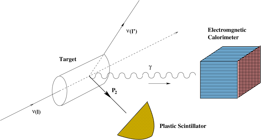
Figure 5.7: A pictorial description of the DVNS experimental setup, where the recoiled nucleon is detected in coincidence with a final state photon.

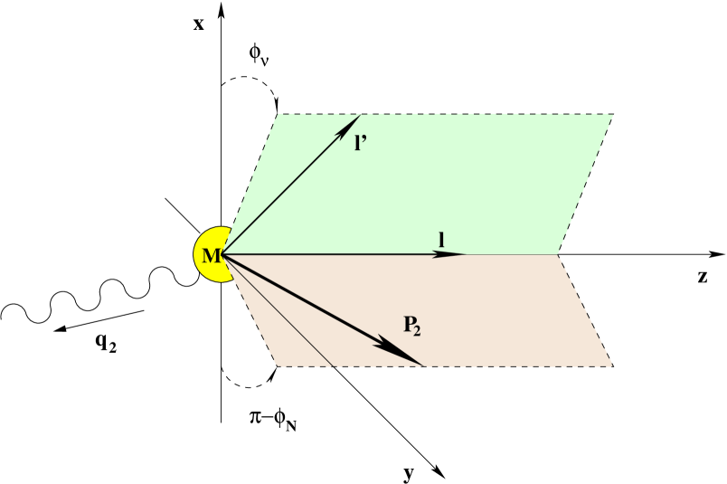
Figure 5.8: Kinematics of the process $\nu(l)N(P_{1})\rightarrow\nu(l^{\prime})N(P_{2})\gamma(q_{2})$

We will be using the relations

$$\bar{q}^{2}=-\frac{1}{2}q_{1}^{2}\left(1-\frac{\Delta^{2}}{2q_{1}^{2}}\right)\approx\frac{1}{2}Q^{2}$$

$$\xi=\frac{x\left(1-\frac{\Delta^{2}}{2q_{1}^{2}}\right)}{2-x\left(1-\frac{\Delta^{2}}{2q_{1}^{2}}\right)}\approx\frac{2x}{2-x}$$

in the final computation of the cross section. It is also important to note that $\Delta^{2}$ has to satisfy a kinematical constraint

$$\Delta^{2}_{min}=-\frac{M^{2}x^{2}}{1-x+\frac{xM^{2}}{Q^{2}}}\left(1+{\cal O}\left(\frac{M^{2}}{Q^{2}}\right)\right)\,.$$ (5.68)

One possible cross section to study, in analogy to the DVCS case [119], is the following

$$\frac{d\sigma}{dxdQ^{2}d|\Delta^{2}|d\phi_{r}}=\frac{y}{Q^{2}}\frac{d\sigma}{dxdyd|\Delta^{2}|d\phi_{r}}=\frac{xy^{2}}{8\pi Q^{4}}\left(1+\frac{4M^{2}x^{2}}{Q^{2}}\right)^{-\frac{1}{2}}|{\cal M}_{fi}|^{2}.$$ (5.69)

where $\phi_{r}$ is the angle between the lepton and the hadron scattering planes. To proceed we also need the relations

$$l\cdot n=\left[\frac{Q^{2}}{2xy}-\frac{(1+\xi)}{2\xi}\frac{Q^{2}}{2}\right]\chi,$$

$$l\cdot\tilde{n}=\frac{Q^{2}}{2\xi}+\frac{Q^{2}}{4\xi^{2}}\left[\frac{Q^{2}}{2xy}-\frac{(1+\xi)}{2\xi}\frac{Q^{2}}{2}\right]\chi,$$

$$n\cdot q_{1}=\frac{2x}{x-2},\hskip 14.22636pt\tilde{n}\cdot q_{1}=Q^{2}\frac{(2-x)}{8x},$$

where $\chi$ is given by

$$\chi=\frac{\xi}{\frac{1+\xi}{2}\frac{Q^{2}}{4\xi}+\frac{\xi(1-\xi)}{2}\frac{\overline{M}^{2}}{2}}\,\,.$$ (5.71)

After some manipulations we obtain a simplified expression for $|{\cal M}_{fi}|^{2}$, similarly to eq. (5.47)

$$|{\cal M}_{fi}|^{2} = \int_{-1}^{1}dz\int_{-1}^{1}dz^{\prime}\left[A_{1}(z,z^{\prime},x,t,Q^{2})\alpha(z)\alpha^{*}(z^{\prime})+A_{2}(z,z^{\prime},x,t,Q^{2})\beta(z)\beta^{*}(z^{\prime})\right]$$ (5.72)

$$\times \left[-2Q^{2}\,(4M^{2}-t)\,(x-2)^{2}\,(x-1)\,x^{2}y+(t-4M^{2})^{2}\,(x-1)^{2}\,x^{4}y^{2}\right.$$

$$+ \left.Q^{4}(x-2)^{4}\,(2-2y+y^{2})\right]$$

$$\times \left[2M^{2}({M_{Z}}^{2}+Q^{2})^{2}\,(x-2)^{2}\,[Q^{2}(x-2)^{2}-(4M^{2}-t)(-1+x)x^{2}]^{2}y^{2}\right]^{-1}$$

where $A_{1}(z,z^{\prime},x,t,Q^{2})$ and $A_{2}(z,z^{\prime},x,t,Q^{2})$ are functions of the invariants of the process and of the entire set of GPD’s. Their explicit form is given in Appendix D. As we have already mentioned, the $(z,z^{\prime})$ integration is be done by using the Feynman prescription to extract the phases and then using the distributional identities (LABEL:rex1)and (LABEL:rex2). For numerical accuracy we have discretized the final integrals by finite element methods, as shown in Appendix C.

Figure 5.9: DVCS cross section at $x=0.1$ and center of mass energy $ME=10$ GeV² using the profile (5.57).

Figure 5.10: DVCS cross section at $x=0.2$ and center of mass energy $ME=10$ GeV² using the profile (5.57).

Figure 5.11: DVCS cross section at $x=0.3$ and center of mass energy $ME=10$ GeV² using the profile (5.57).

Figure 5.12: DVCS cross section at $x=0.1$ and center of mass energy $ME=27$ GeV² using the profile (5.57).

Figure 5.13: DVCS cross section at $x=0.3$ and center of mass energy $ME=10$ GeV² with NPD functions generated by the profile function (5.59).

Figure 5.14: DVCS cross section at $x=0.3$ and center of mass energy $ME=27$ GeV² with NPD functions generated by the profile function (5.59).

Figure 5.15: DVCS cross sections at $x=0.2$ and center of mass energy $ME=27$ GeV². $\tilde{\sigma}$ using profile (5.59).

We have plotted the differential cross section as a function of $Q^{2}$, for various values of $\Delta^{2}$ and at fixed $x$ values. We have used both the profile given by (5.57) (Figs. 5.9-5.12) and the one given in eq. (5.59) (Figs. 5.13 and 5.14) and their direct comparison in a specific kinematical region (Fig. 5.15). The different profiles generate differences in the cross sections especially for larger $\Delta^{2}$ values. Notice also that the DVNS cross section decreases rather sharply with $\Delta^{2}$, at the same time it increases appreciably with $x$. The results shown are comparable with other cross sections evaluated in the quasi-elastic region ($\approx 10^{-5}$ nb) for charged and neutral current interactions, and appear to be sizeable. Coherence effects due to neutral current interactions with heavy nuclei, in particular with the neutron component may substantially increase the size of the cross sections, with an enhancement proportional to $N^{2}$, where $N$ is the number of neutrons [120], though an accurate quantification of these effects requires a special study [121] which is underway. It is worth to emphasize that in the past this contribution had never been included in the study of neutrino-nucleon interactions since very little was known about the intermediate energy kinematics in QCD from the point of view of factorization. It seems obvious to us that with the new developments now taking place in the study of QCD at intermediate energy, especially in the case of the generalized Bjorken region, of which the deeply virtual scattering limit is just a special case, it will be of wide interest to quantify with accuracy the role of these new contributions for neutrino factories. In general, one expects that electromagnetic effects are suppressed compared to the standard (hadronic) deeply inelastic cross section, and this has led in the past to a parameterization of the intermediate energy cross section as either dominated by the quasi elastic region and/or by the DIS region at higher energies, as we have mentioned in our introduction. However, the exclusive cross section has some special positive features, one of them being to provide a clean signal for the detection of weakly interacting particles, and we expect that this aspect is going to be of relevance at experimental level.

5.8 Conclusions

We have presented an extension of the standard DVCS process to the case of one neutral current exchange, describing the scattering of a neutrino off a proton in the parton model. We have described the leading twist behaviour of the cross section; we have found that this is comparable to other typical neutrino cross sections and discussed its forward or DIS limit. We have presented a complete formalism for the study of these processes in the parton model. The process is the natural generalization of DIS with neutral currents and relies on the notion of Generalized Parton Distributions, new constructs in the parton model which have received considerable attention in recent years. The possible applications of these new processes are manifold and we hope to return in the near future with a discussion of some of the issues not addressed in this thesis.

5.9 Appendix A

The collinear expansion of the internal loop momentum $k$ allows to identify the light cone operators appearing in the process at leading twist. We recall at this point that the analysis of the hand-bag contribution is carried out exactly as in the electromagnetic case.

To perform the collinear expansion and isolate the light-cone correlators of DVNS from the hand-bag contribution we use the relation

$$\int\frac{d\lambda\ dx}{2\pi}e^{i\lambda(x-k\cdot n)}=1$$ (5.73)

inside the expression of $T^{\mu\nu}$ in order to obtain

$$T^{\mu\nu} = -\int\frac{d^{4}k}{(2\pi)^{4}}\int\frac{d\lambda\ dx}{2\pi}e^{i\lambda(x-k\cdot n)}$$

$$Tr\left\{\left[\gamma^{\nu}\frac{i}{\hbox to0.0pt{/\hss}k-\alpha\hbox to0.0pt{/\hss}\Delta+\hbox to0.0pt{/\hss}q_{1}+i\epsilon}\gamma^{\mu}+\gamma^{\mu}\frac{i}{\hbox to0.0pt{/\hss}k+(1-\alpha)\hbox to0.0pt{/\hss}\Delta-\hbox to0.0pt{/\hss}q_{1}+i\epsilon}\gamma^{\nu}\right]\underline{M}(k)\right\}$$

and therefore

$$T^{\mu\nu} = -\int\frac{dk\cdot n\ dk\cdot\tilde{n}\ dk_{\perp}^{2}}{(2\pi)^{4}}\int\frac{d\lambda\ dx}{2\pi}e^{i\lambda(x-k\cdot n)}\int d^{4}z\ e^{ik\cdot z}$$

$$Tr\left\{\left[\gamma^{\nu}\frac{i}{\hbox to0.0pt{/\hss}k-\alpha\hbox to0.0pt{/\hss}\Delta+\hbox to0.0pt{/\hss}q_{1}+i\epsilon}\gamma^{\mu}+\gamma^{\mu}\frac{i}{\hbox to0.0pt{/\hss}k+(1-\alpha)\hbox to0.0pt{/\hss}\Delta-\hbox to0.0pt{/\hss}q_{1}+i\epsilon}\gamma^{\nu}\right]\right.$$

$$\cdot \left.\langle P^{\prime}|\overline{\psi}(-\alpha z)\psi((1-\alpha)z)|P\rangle\right\}.$$

Keeping the leading terms for the loop momenta

$$k^{\mu}-\alpha\Delta^{\mu}+q_{1}^{\mu} = \tilde{n}^{\mu}\left(k\cdot n+2\alpha\xi-2\xi\right)+n^{\mu}\left(k\cdot\tilde{n}-{\alpha}\xi\overline{M}^{2}+\frac{Q^{2}}{4\xi}\right)$$

$$k^{\mu}+(1-\alpha)\Delta^{\mu}-q_{1}^{\mu} = \tilde{n}^{\mu}\left(k\cdot n-2(1-\alpha)\xi+2\xi\right)+n^{\mu}\left(k\cdot\tilde{n}+2(1-\alpha)\xi\overline{M}^{2}-\frac{Q^{2}}{4\xi}\right)$$

we thus obtain

$$T^{\mu\nu} = -\int\frac{d(k\cdot n)\ d(k\cdot\tilde{n})\ dk_{\perp}^{2}}{(2\pi)^{4}}\int\frac{d\lambda\ dx}{2\pi}e^{i\lambda(x-k\cdot n)}\int d^{4}z\ e^{ik\cdot z}$$

$$Tr\left\{\left[\gamma^{\nu}\frac{\hbox to0.0pt{/\hss}\tilde{n}}{2\left(k\cdot\tilde{n}-{\alpha}\xi\overline{M}^{2}+\frac{Q^{2}}{4\xi}\right)}\gamma^{\mu}+\gamma^{\mu}\frac{\hbox to0.0pt{/\hss}\tilde{n}}{2\left(k\cdot\tilde{n}+(1-\alpha){\xi}\overline{M}^{2}-\frac{Q^{2}}{4\xi}\right)}\gamma^{\nu}\right.\right.$$

$$+ \left.\left.\gamma^{\nu}\frac{\hbox to0.0pt{/\hss}n}{2\left(k\cdot n+2\alpha\xi-2\xi\right)}\gamma^{\mu}+\gamma^{\mu}\frac{\hbox to0.0pt{/\hss}n}{2\left(k\cdot n-2(1-\alpha)\xi+2\xi\right)}\gamma^{\nu}\right]\right.$$

$$\cdot \left.\langle P^{\prime}|\overline{\psi}(-\alpha z)\psi((1-\alpha)z)|P\rangle\right\}.$$

We expand

$$k\cdot z = (k\cdot n)\ (\tilde{n}\cdot z)+(k\cdot\tilde{n})\ (n\cdot z)-\vec{k}_{\perp}\cdot\vec{z}_{\perp}$$

and choose $\alpha=1/2$. These expansions are introduced in eq. 5.21 and after some manipulations the tensor $T$ now becomes

$$T^{\mu\nu}|_{\alpha=1/2} = -\int\frac{d(k\cdot n)\ d(k\cdot\tilde{n})\ dk_{\perp}^{2}}{(2\pi)^{4}}\int\frac{d\lambda\ dx}{2\pi}e^{i\lambda(x-k\cdot n)}\int d^{4}z\ e^{ik\cdot z}$$

$$Tr\left\{\left[\gamma^{\nu}\frac{\hbox to0.0pt{/\hss}\tilde{n}}{2\left(k\cdot\tilde{n}-\frac{\alpha}{2}\xi\overline{M}^{2}+\frac{Q^{2}}{2\xi}\right)}\gamma^{\mu}+\gamma^{\mu}\frac{\hbox to0.0pt{/\hss}\tilde{n}}{2\left(k\cdot\tilde{n}+(1-\alpha){\xi}\overline{M}^{2}-\frac{Q^{2}}{4\xi}\right)}\gamma^{\nu}\right.\right.$$

$$+ \left.\left.\gamma^{\nu}\frac{\hbox to0.0pt{/\hss}n}{2\left(k\cdot n+2\alpha\xi-2\xi\right)}\gamma^{\mu}+\gamma^{\mu}\frac{\hbox to0.0pt{/\hss}n}{2\left(k\cdot n-2(1-\alpha)\xi+2\xi\right)}\gamma^{\nu}\right]\right.$$

$$\cdot \left.\langle P^{\prime}|\overline{\psi}(-\alpha z)\psi((1-\alpha)z)|P\rangle\right\}.$$

We also recall that the expansion of the matrix element $\underline{M}(k)$ proceeds also in this case as in the electromagnetic case

$$\underline{M}_{ab}^{(i)}(k) = \int d^{4}ye^{ik\cdot y}\langle P^{\prime}|\overline{\psi}_{a}^{(i)}(-\alpha y)\psi_{b}^{(i)}((1-\alpha)y)|P\rangle=A_{1}\tilde{n}\hskip-6.0pt/\hskip 6.0pt+A_{2}\gamma_{5}\tilde{n}\hskip-6.0pt/\hskip 6.0pt+...$$ (5.74)

where the ellipses refer to terms which are of higher twist or disappear in the trace of the diagram.

5.10 Appendix B

The last ingredients needed in the construction of the input distribution functions are the form factors $F^{i}_{1}$ and $F^{i}_{2}$. From experimental measurements we know, by a dipole parametrization in the small $\Delta^{2}$ region, that

$$G_{E}^{p}(\Delta^{2})=(1+\kappa_{p})^{-1}G_{M}^{p}(\Delta^{2})=\kappa_{n}^{-1}G_{M}^{n}(\Delta^{2})=\left(1-\frac{\Delta^{2}}{m_{V}^{2}}\right)^{-2},\qquad G_{E}^{n}(\Delta^{2})=0,$$ (5.75)

where the electric, $G_{E}^{i}(\Delta^{2})=F_{1}^{i}(\Delta^{2})+\frac{\Delta^{2}}{4M^{2}}F_{2}^{i}(\Delta^{2})$, and magnetic form factors $G_{M}^{i}(\Delta^{2})=F_{1}^{i}(\Delta^{2})+F_{2}^{i}(\Delta^{2})$ are usually parametrized in terms of a cutoff mass $m_{V}=0.84\,{\rm GeV}$.
For non-polarized GPD’s the valence $u$ and $d$ quark form factors in the proton can be easily extracted from $F_{I}^{({p\atop n})}=2\left({Q_{u}\atop Q_{d}}\right)F_{I}^{u}+\left({Q_{d}\atop Q_{u}}\right)F_{I}^{d}$ and given exclicitely by

$$2F^{u}_{I}(\Delta^{2})=2F_{I}^{p}(\Delta^{2})+F_{I}^{n}(\Delta^{2}),\qquad F^{d}_{I}(\Delta^{2})=F_{I}^{p}(\Delta^{2})+2F_{I}^{n}(\Delta^{2}),\quad\mbox{for}\quad I=1,2.$$ (5.76)

This exploits the fact that proton and neutron form an iso-spin doublet.

At the scale $m_{A}=0.9$ GeV one can get

$$G^{i}_{1}(\Delta^{2})=\left(1-\frac{\Delta^{2}}{m_{A}^{2}}\right)^{-2}$$ (5.77)

for the valence quarks. For the form factors $F$ we obtain

$$F_{1}^{u}=-\frac{A\Delta^{2}}{M^{2}(1-B\Delta^{2})^{2}\left(-1+\frac{\Delta^{2}}{4M^{2}}\right)}+\frac{1-\frac{C\Delta^{2}}{M^{2}\left(1-\frac{\Delta^{2}}{4M^{2}}\right)}}{(1-B\Delta^{2})^{2}},$$

$$F_{2}^{u}=\frac{D}{(1-B\Delta^{2})^{2}\left(1-\frac{\Delta^{2}}{4M^{2}}\right)},$$

$$F_{1}^{d}=-\frac{E\Delta^{2}}{M^{2}(1-B\Delta^{2})^{2}\left(-1+\frac{\Delta^{2}}{4M^{2}}\right)}+\frac{1-\frac{C\Delta^{2}}{M^{2}\left(1-\frac{\Delta^{2}}{4M^{2}}\right)}}{(1-B\Delta^{2})^{2}},$$

$$F_{2}^{d}=\frac{F}{(1-B\Delta^{2})^{2}\left(1-\frac{\Delta^{2}}{4M^{2}}\right)},$$

where

$$A=0.238\hskip 28.45274ptB=1.417\hskip 28.45274ptC=0.447,$$

$$D=0.835\hskip 28.45274ptE=0.477\hskip 28.45274ptF=0.120.$$ (5.79)

5.11 Appendix C

In this section we illustrate an analytical computation of the integrals by discretization, using finite elements method. We want to approximate with high numerical accuracy integrals of the form

$$P.V.\int_{-1}^{1}\frac{H(z)dz}{z-\xi}=\int_{-1}^{\xi}dz\frac{H(z)-H(\xi)}{z-\xi}+\int_{\xi}^{1}dz\frac{H(z)-H(\xi)}{z-\xi}+H(\xi)\ln\left|\frac{\xi-1}{\xi+1}\right|.$$ (5.80)

For this purpose we start by choosing a grid on the interval $(-1=x_{0},.....,x_{n+1}=\xi)$ and define

$$J_{1}=\int_{-1}^{\xi}dz\frac{H(z)-H(\xi)}{z-\xi}=\sum_{j=0}^{n}\int_{x_{j}}^{x_{j+1}}dx\frac{H(x)-H(\xi)}{x-\xi}\,.$$ (5.81)

Performing a simple linear interpolation we get

$$J_{1} = \sum_{j=0}^{n-1}\int_{x_{j}}^{x_{j+1}}\left\{H(x_{j})\left[\frac{x_{j+1}-x}{x_{j+1}-x_{j}}\right]+H(x_{j+1})\left[\frac{x-x_{j}}{x_{j+1}-x_{j}}\right]\right\}\frac{dx}{x-\xi}\,\,$$ (5.82)

$$+ \int_{x_{n}}^{\xi}\left\{H(x_{n})\left[\frac{\xi-x}{\xi-x_{n}}\right]+H(\xi)\left[\frac{x-x_{n}}{\xi-x_{n}}\right]\right\}\frac{dx}{x-\xi}-\int_{-1}^{\xi}dx\frac{H(\xi)}{x-\xi}\,\,.$$

After the integration we are left with

$$J_{1} = \sum_{j=0}^{n-1}H(x_{j})\left[-1+\left(\frac{x_{j+1}-\xi}{x_{j+1}-x_{j}}\right)\ln\left|\frac{x_{j+1}-\xi}{x_{j}-\xi}\right|\right]$$ (5.83)

$$+ \sum_{j=0}^{n-1}H(x_{j+1})\left[1+\left(\frac{\xi-x_{j}}{x_{j+1}-x_{j}}\right)\ln\left|\frac{x_{j+1}-\xi}{x_{j}-\xi}\right|\right]$$

$$- \sum_{j=0}^{n-1}H(\xi)\ln\left|\frac{x_{j+1}-\xi}{x_{j}-\xi}\right|-H(x_{n})+H(\xi)\,\,.$$

Now, moving to the integral in the interval $(\xi,1)$, we introduce a similar grid of equally spaced points $(\xi=y_{0},......,y_{n+1}=1)$ and define the integral

$$J_{2}=\int_{\xi}^{1}dz\frac{H(z)-H(\xi)}{z-\xi}=\sum_{j=0}^{n}\int_{y_{j}}^{y_{j+1}}dy\frac{H(y)-H(\xi)}{y-\xi}.$$ (5.84)

As above, after isolating the singularity we obtain

$$J_{2} = \sum_{j=1}^{n}\int_{y_{j}}^{y_{j+1}}\left\{H(y_{j})\left[1-\frac{y-y_{j}}{y_{j+1}-y_{j}}\right]+H(y_{j+1})\left[\frac{y-y_{j}}{y_{j+1}-y_{j}}\right]\right\}\frac{dy}{y-\xi}\,\,$$ (5.85)

$$+ H(y_{1})+H(\xi)\int_{\xi}^{y_{1}}\left[\frac{y_{1}-y}{y_{1}-\xi}\right]dy\,\,-\,\,\int_{\xi}^{1}dy\frac{H(\xi)}{y-\xi}\,\,.$$

Again, performing the integrations we obtain

$$J_{2} = \sum_{j=1}^{n}H(y_{j})\left[-1+\left(\frac{y_{j+1}-\xi}{y_{j+1}-y_{j}}\right)\ln\left|\frac{y_{j+1}-\xi}{y_{j}-\xi}\right|\right]$$ (5.86)

$$+ \sum_{j=1}^{n}H(y_{j+1})\left[1+\left(\frac{\xi-y_{j}}{y_{j+1}-y_{j}}\right)\ln\left|\frac{y_{j+1}-\xi}{y_{j}-\xi}\right|\right]$$

$$- \sum_{j=1}^{n}H(\xi)\ln\left|\frac{y_{j+1}-\xi}{y_{j}-\xi}\right|+H(y_{1})-H(\xi)\,\,.$$

Collecting our results, at the end we obtain

$$P.V.\int_{-1}^{1}\frac{H(z)dz}{z-\xi}=J_{1}+J_{2}+H(\xi)\ln\left|\frac{\xi-1}{\xi+1}\right|\,.$$ (5.87)

We can use the same strategy for the integrals of “$+$” type defined as follows

$$P.V.\int_{-1}^{1}\frac{H(z)dz}{z+\xi}=\int_{-1}^{-\xi}dz\frac{H(z)-H(-\xi)}{z+\xi}+\int_{-\xi}^{1}dz\frac{H(z)-H(-\xi)}{z+\xi}+H(-\xi)\ln\left|\frac{\xi+1}{\xi-1}\right|.$$ (5.88)

This time we call our final integrals $X_{1}$ and $X_{2}$. They are given by the expressions

$$X_{1} = \sum_{j=0}^{n-1}H(x_{j})\left[-1+\left(\frac{x_{j+1}+\xi}{x_{j+1}-x_{j}}\right)\ln\left|\frac{x_{j+1}+\xi}{x_{j}+\xi}\right|\right]$$ (5.89)

$$+ \sum_{j=0}^{n-1}H(x_{j+1})\left[1+\left(\frac{-\xi-x_{j}}{x_{j+1}-x_{j}}\right)\ln\left|\frac{x_{j+1}+\xi}{x_{j}+\xi}\right|\right]$$

$$- \sum_{j=0}^{n-1}H(-\xi)\ln\left|\frac{x_{j+1}+\xi}{x_{j}+\xi}\right|-H(x_{n})+H(-\xi)\,\,,$$

with a discretization supported in the $(-1=x_{0},.....,x_{n+1}=\xi)$ grid, and

$$X_{2} = \sum_{j=1}^{n}H(y_{j})\left[-1+\left(\frac{y_{j+1}+\xi}{y_{j+1}-y_{j}}\right)\ln\left|\frac{y_{j+1}+\xi}{y_{j}+\xi}\right|\right]$$ (5.90)

$$+ \sum_{j=1}^{n}H(y_{j+1})\left[1+\left(\frac{-\xi-y_{j}}{y_{j+1}-y_{j}}\right)\ln\left|\frac{y_{j+1}+\xi}{y_{j}+\xi}\right|\right]$$

$$- \sum_{j=1}^{n}H(-\xi)\ln\left|\frac{y_{j+1}+\xi}{y_{j}+\xi}\right|+H(y_{1})-H(-\xi)\,\,.$$

on the $(-\xi=y_{0},.....,y_{n+1}=1)$ grid. As a final result for the “$+$” integral we get

$$P.V.\int_{-1}^{1}\frac{H(z)dz}{z+\xi}=X_{1}+X_{2}+H(-\xi)\ln\left|\frac{\xi+1}{\xi-1}\right|\,.$$ (5.91)

5.12 Appendix D

In this section we will present the full expression of the functions $A_{1}$ and $A_{2}$ which appear in the squared amplitude

$$A_{1}(z,z^{\prime}x,t,Q^{2}) = \tilde{g}^{4}Q^{2}\left.\left[4g_{d}^{2}[\tilde{E}_{d}^{\prime}(4\tilde{H}_{d}M^{2}+\tilde{E}_{d}t)x^{2}\right.\right.$$

$$+\left.\left.4\tilde{H}_{d}^{\prime}M^{2}(4\tilde{H}_{d}(x-1)+\tilde{E}_{d}x^{2})]\right.\right.$$

$$+\left.\left.4g_{d}g_{u}[(4\tilde{E}_{u}^{\prime}\tilde{H}_{d}M^{2}+4\tilde{E}_{d}^{\prime}\tilde{H}_{u}M^{2}+\tilde{E}_{u}^{\prime}\tilde{E}_{d}t+\tilde{E}_{d}^{\prime}\tilde{E}_{u}t)x^{2}\right.\right.$$

$$+\left.\left.4\tilde{H}_{u}^{\prime}M^{2}(4\tilde{H}_{d}(x-1)+\tilde{E}_{d}x^{2})+4\tilde{H}_{d}^{\prime}M^{2}(4\tilde{H}_{u}(x-1)+\tilde{E}_{u}x^{2})]\right.\right.$$

$$+\left.\left.D_{v}U_{v}g_{d}g_{u}[4E_{u}^{\prime}E_{d}t+4E_{d}^{\prime}E_{u}t-4E_{u}^{\prime}E_{d}tx-4E_{d}^{\prime}E_{u}tx+4E_{u}^{\prime}E_{d}M^{2}x^{2}\right.\right.$$

$$+\left.\left.4E_{d}^{\prime}E_{u}M^{2}x^{2}+4E_{u}^{\prime}H_{d}M^{2}x^{2}+4E_{d}^{\prime}H_{u}M^{2}x^{2}+E_{u}^{\prime}E_{d}tx^{2}+E_{d}^{\prime}E_{u}tx^{2}\right.\right.$$

$$+\left.\left.4H_{u}^{\prime}M^{2}(4H_{d}(x-1)+E_{d}x^{2})+4H_{d}^{\prime}M^{2}(4H_{u}(x-1)+E_{u}x^{2})]\right.\right.$$

$$+\left.\left.g_{u}^{2}[4E_{u}^{\prime}E_{u}tU_{v}^{2}-4E_{u}^{\prime}E_{u}tU_{v}^{2}x+16\tilde{E}_{u}^{\prime}\tilde{H}_{u}M^{2}x^{2}+4\tilde{E}_{u}^{\prime}\tilde{E}_{u}tx^{2}\right.\right.$$

$$+\left.\left.4E_{u}^{\prime}E_{u}M^{2}U_{v}^{2}x^{2}+4E_{u}^{\prime}H_{u}M^{2}U_{v}^{2}x^{2}+E_{u}^{\prime}E_{u}tU_{v}^{2}x^{2}+16\tilde{H}_{u}^{\prime}M^{2}(4\tilde{H}_{u}(x-1)+\tilde{E}_{u}x^{2})\right.\right.$$

$$+\left.\left.4H_{u}^{\prime}M^{2}U_{v}^{2}(4H_{u}(x-1)+E_{u}x^{2})]\right.\right.$$

$$+\left.\left.D_{v}^{2}g_{d}^{2}[4H_{d}^{\prime}M^{2}(4H_{d}(x-1)+E_{d}x^{2})+E_{d}^{\prime}(4H_{d}M^{2}x^{2}+E_{d}(t\,(x-2)^{2}+4M^{2}x^{2}))]\right]\right.$$

and for $A_{2}(z,z^{\prime},x,t)$ we get a similar result

$$A_{2}(z,z^{\prime},x,t,Q^{2}) = \left.4\tilde{g}^{4}Q^{2}\left[g_{d}g_{u}[4E^{\prime}_{u}E_{d}t+4E^{\prime}_{d}E_{u}t-16D_{v}\tilde{H}^{\prime}_{u}\tilde{H}_{d}M^{2}U_{v}-16D_{v}\tilde{H}^{\prime}_{d}\tilde{H}_{u}M^{2}U_{v}-4E^{\prime}_{u}E_{d}tx\right.\right.$$

$$- \left.\left.4E^{\prime}_{d}E_{u}tx+16D_{v}\tilde{H}_{u}\tilde{H}_{d}M^{2}U_{v}x+16D_{v}\tilde{H}^{\prime}_{d}\tilde{H}_{u}M^{2}U_{v}x+4E^{\prime}_{u}E_{d}M^{2}x^{2}+4E^{\prime}_{d}E_{u}M^{2}x^{2}\right.\right.$$

$$+ \left.\left.4E^{\prime}_{u}H_{d}M^{2}x^{2}+4E^{\prime}_{d}H_{u}M^{2}x^{2}+E^{\prime}_{u}E_{d}tx^{2}+E^{\prime}_{d}E_{u}tx^{2}+4D_{v}\tilde{E}_{u}\tilde{H}^{\prime}_{d}M^{2}U_{v}x^{2}\right.\right.$$

$$+ \left.\left.4D_{v}\tilde{E}_{d}\tilde{H}^{\prime}_{u}M^{2}U_{v}x^{2}+4D_{v}\tilde{E}^{\prime}_{u}\tilde{H}_{d}M^{2}U_{v}x^{2}+4D_{v}\tilde{E}^{\prime}_{d}\tilde{H}_{u}M^{2}U_{v}x^{2}+D_{v}\tilde{E}^{\prime}_{u}\tilde{E}_{d}tU_{v}x^{2}\right.\right.$$

$$+ \left.\left.D_{v}\tilde{E}^{\prime}_{d}\tilde{E}_{u}tU_{v}x^{2}+4H^{\prime}_{u}M^{2}(4H_{d}(x-1)+E_{d}x^{2})+4H^{\prime}_{d}M^{2}(4H_{u}(x-1)+E_{u}x^{2})]\right.\right.$$

$$+ \left.\left.g_{d}^{2}[4H^{\prime}_{d}M^{2}(4H_{d}(x-1)+E_{d}x^{2})+D_{v}^{2}(\tilde{E}^{\prime}_{d}(4\tilde{H}_{d}M^{2}+\tilde{E}_{d}t)x^{2}\right.\right.$$

$$+ \left.\left.4\tilde{H}^{\prime}_{d}M^{2}(4\tilde{H}_{d}(x-1)+\tilde{E}_{d}x^{2}))+E^{\prime}_{d}(4H_{d}M^{2}x^{2}+E_{d}(t(x-2)^{2}+4M^{2}x^{2}))]\right.\right.$$

$$+ \left.\left.g_{u}^{2}[4H^{\prime}_{u}M^{2}(4H_{u}(x-1)+E_{u}x^{2})+U_{v}^{2}(\tilde{E}^{\prime}_{u}(4\tilde{H}_{u}M^{2}+\tilde{E}_{u}t)x^{2}\right.\right.$$

$$+ \left.\left.4\tilde{H}^{\prime}_{u}M^{2}(4\tilde{H}_{u}(x-1)+\tilde{E}_{u}x^{2}))+E^{\prime}_{u}(4H_{u}M^{2}x^{2}+E_{u}(t(x-2)^{2}+4M^{2}x^{2}))]\right]\right..$$

Chapter 6 Leading Twist Amplitudes for Exclusive Neutrino Interactions in the Deeply Virtual Limit

6.1 Introduction and Motivations

In the prevoius chapter we have pointed out [122] that exclusive processes of DVCS-type (Deeply Virtual Compton Scattering) could be relevant also in the theoretical study of the exclusive neutrino/nucleon interaction. Thanks to the presence of an on-shell photon emitted in the final state, this particle could be tagged together with the recoiling nucleon in a large underground detector in order to trigger on the process and exclude contamination from other backgrounds. With these motivations, a study of the $\nu N\to\nu N\gamma$ process has been performed in [122]. The process is mediated by a neutral current and is particularly clean since there is no Bethe-Heitler contribution. It has been termed Deeply Virtual Neutrino Scattering or DVNS and requires in its partonic description the electroweak analogue of the “non-forward parton distributions”, previously introduced in the study of DVCS.

In this section we extend that analysis and provide, in part, a generalization of those results to the charged current case. Our treatment, here, is purposely short. The method that we use for the study of the charged processes is based on the formalism of the non-local operator product expansion and the technique of the harmonic polynomials, which allows to classify the various contributions to the interaction in terms of operators of a definite geometrical twist [123]. We present here a classification of the leading twist amplitudes of the charged process while a detailed phenomenological analysis useful for future experimental searches will be given elsewhere.

6.2 The Generalized Bjorken Region and DVCS

Fig. 5.1 illustrates the process that we are going to study, where a neutrino of momentum $l$ scatters off a nucleon of momentum $P_{1}$ via a neutral or a charged current interaction; from the final state a photon and a nucleon emerge, of momenta $q_{2}$ and $P_{2}$ respectively, while the momenta of the final lepton is $l^{\prime}$. We recall that Compton scattering has been investigated in the near past by several groups, since the original works [100, 101, 102]. A previous study of the Virtual Compton process in the generalized Bjorken region, of which DVCS is just a particular case, can be found in [103]. From the hadronic side, the description of the interaction proceeds via new constructs of the parton model termed generalized parton distributions (GPD) or also non-forward parton distributions. The kinematics for the study of GPD’s is characterized by a deep virtuality of the exchanged photon in the initial interaction ($\nu+p\to\nu+p+\gamma$) ( $Q^{2}\approx$ 2 GeV²), with the final state photon kept on-shell; large energy of the hadronic system ($W^{2}>6$ GeV²) above the resonance domain and small momentum transfers $|t|<1$ GeV². In the electroweak case, photon emission can occur from the final state electron (in the case of charged current interactions) and provides an additional contribution to the virtual Compton amplitude. We choose symmetric defining momenta and use as independent variables the average of the hadron and gauge bosons momenta

$$P_{1,2}=\bar{P}\mp\frac{\Delta}{2}\,\,\,\,\,\,\,\,q_{1,2}=q\pm\frac{\Delta}{2},$$ (6.1)

with $\Delta=P_{2}-P_{1}$ being the momentum transfer. Clearly

$$\bar{P}\cdot\Delta=0,\,\,\,\,\,\bar{P}^{2}=M^{2}-\frac{\Delta^{2}}{4}$$ (6.2)

and $M$ is the nucleon mass. There are two scaling variables which are identified in the process, since 3 scalar products can grow large in the generalized Bjorken limit: $q^{2}$, $\Delta\cdot q$, $\bar{P}\cdot q$.

The momentum transfer $\Delta^{2}$ is a small parameter in the process. Momentum asymmetries between the initial and the final state nucleon are measured by two scaling parameters, $\xi$ and $\eta$, related to ratios of the former invariants

$$\xi=-\frac{q^{2}}{2\bar{P}\cdot q} \eta=\frac{\Delta\cdot q}{2\bar{P}\cdot q}$$ (6.3)

where $\xi$ is a variable of Bjorken type, expressed in terms of average momenta rather than nucleon and gauge bosons momenta. The standard Bjorken variable $x=-q_{1}^{2}/(2P_{1}\cdot q_{1})$ is trivially related to $\xi$ in the $t=0$ limit and in the DVCS case $\eta=-\xi$.

Notice also that the parameter $\xi$ measures the ratio between the plus component of the momentum transfer and the average momentum.

$\xi$, therefore, parametrizes the large component of the momentum transfer $\Delta$, which can be generically described as

$$\Delta=-2\xi\bar{P}-{\Delta}_{\perp}$$ (6.4)

where all the components of ${\Delta}_{\perp}$ are $O\left(\sqrt{|\Delta^{2}|}\right)$.

6.3 Bethe-Heitler Contributions

Prior to embark on the discussion of the virtual Compton contribution, we quote the result for the Bethe-Heitler (BH) subprocess, which makes its first appearance in the charged current case, since a real photon can be radiated off the leg of the final state lepton. The amplitude of the BH contribution for a $W^{+}$ exchange is as follows

$$T_{BH}^{W^{+}}=-|e|\frac{g}{2\sqrt{2}}\frac{g}{\sqrt{2}}\overline{u}(l^{\prime})\left[\gamma^{\mu}\frac{(l\hskip-6.0pt/\hskip 6.0pt-\Delta\hskip-6.0pt/\hskip 6.0pt)}{(l-\Delta)^{2}+i\epsilon}\gamma^{\nu}(1-\gamma^{5})\right]u(l)\frac{D^{\nu\delta}(q_{1})}{\Delta^{2}-M_{W}^{2}+i\epsilon}\epsilon^{*}_{\mu}(q_{2})\times$$

$$\hskip 56.9055pt\overline{U}(P_{2})\left[\left(F_{1}^{u}(\Delta^{2})-F_{1}^{d}(\Delta^{2})\right)\gamma^{\delta}+\left(F_{2}^{u}(\Delta^{2})-F_{2}^{d}(\Delta^{2})\right)i\frac{\sigma^{\delta\alpha}\Delta_{\alpha}}{2M}\right]U(P_{1}),$$

where $\epsilon$ is the polarization vector of the photon and

$$T_{BH}^{W^{-}}=|e|\frac{g}{2\sqrt{2}}\frac{g}{\sqrt{2}}\overline{v}(l)\left[\gamma^{\mu}\frac{(l\hskip-6.0pt/\hskip 6.0pt-\Delta\hskip-6.0pt/\hskip 6.0pt)}{(l-\Delta)^{2}+i\epsilon}\gamma^{\nu}(1-\gamma^{5})\right]v(l^{\prime})\frac{D^{\nu\delta}(q_{1})}{\Delta^{2}-M_{W}^{2}+i\epsilon}\epsilon^{*}_{\mu}(q_{2})\times$$

$$\hskip 56.9055pt\overline{U}(P_{2})\left[\left(F_{1}^{u}(\Delta^{2})-F_{1}^{d}(\Delta^{2})\right)\gamma^{\delta}+\left(F_{2}^{u}(\Delta^{2})-F_{2}^{d}(\Delta^{2})\right)i\frac{\sigma^{\delta\alpha}\Delta_{\alpha}}{2M}\right]U(P_{1})\,$$

for the $W^{-}$ case, with $D^{\nu\delta}(q_{1})/{(\Delta^{2}-M_{W}^{2}+i\epsilon)}$ being the propagator of the W’s and $F_{1,2}$ the usual nucleon form factors (see also [122]).

6.4 Structure of the Compton amplitude for charged and neutral currents

Moving to the Compton amplitude for charged and neutral currents, this can be expressed in terms of the correlator of currents

$$T_{\mu\nu}=i\int d^{4}xe^{iqx}\langle P_{2}|T\left(J_{\nu}^{\gamma}(x/2)J_{\mu}^{W^{\pm},Z_{0}}(-x/2)\right)|P_{1}\rangle\,,$$ (6.7)

where for the charged and neutral currents we have the following expressions

$$J^{\mu Z_{0}}(-x/2)=\frac{g}{2\cos{\theta_{W}}}\overline{\psi}_{u}(-x/2)\gamma^{\mu}(g^{Z}_{uV}+g^{Z}_{uA}\gamma^{5})\psi_{u}(-x/2)+\overline{\psi}_{d}(-x/2)\gamma^{\mu}(g^{Z}_{dV}+g^{Z}_{dA}\gamma^{5})\psi_{d}(-x/2),\,$$

$$J^{\mu W^{+}}(-x/2)=\frac{g}{2\sqrt{2}}\overline{\psi}_{u}(-x/2)\gamma^{\mu}(1-\gamma^{5})U^{*}_{ud}\psi_{d}(-x/2),\,$$

$$J^{\mu W^{-}}(-x/2)=\frac{g}{2\sqrt{2}}\overline{\psi}_{d}(-x/2)\gamma^{\mu}(1-\gamma^{5})U_{du}\psi_{u}(-x/2),\,$$

$$J^{\nu,\gamma}(x/2)=\overline{\psi}_{d}(x/2)\gamma^{\nu}\left(-\frac{1}{3}e\right)\psi_{d}(x/2)+\overline{\psi}_{u}(x/2)\gamma^{\nu}\left(\frac{2}{3}e\right)\psi_{u}(x/2)\,.$$ (6.8)

Here we have chosen a simple representation of the flavour mixing matrix $U^{*}_{ud}=U_{ud}=U_{du}=\cos{\theta_{C}}$, where $\theta_{C}$ is the Cabibbo angle.

The coefficients $g_{V}^{Z}$ and $g_{A}^{Z}$ are

$$g^{Z}_{uV}=\frac{1}{2}+\frac{4}{3}\sin^{2}\theta_{W}\hskip 42.67912ptg^{Z}_{uA}=-\frac{1}{2}$$

$$g^{Z}_{dV}=-\frac{1}{2}+\frac{2}{3}\sin^{2}\theta_{W}\hskip 42.67912ptg^{Z}_{dA}=\frac{1}{2}\,,$$ (6.9)

and

$$g_{u}=\frac{2}{3}, g_{d}=\frac{1}{3}$$ (6.10)

are the absolute values of the charges of the up and down quarks in units of the electron charge. A short computation gives

$$\langle P_{2}|T\left(J_{\nu}^{\gamma}(x/2)J_{\mu}^{Z_{0}}(-x/2)\right)|P_{1}\rangle=$$

$$\langle P_{2}|\overline{\psi}_{u}(x/2)g_{u}\gamma_{\nu}S(x)\gamma_{\mu}(g^{Z}_{uV}+g^{Z}_{uA}\gamma^{5})\psi_{u}(-x/2)-$$

$$\hskip 22.76228pt\overline{\psi}_{d}(x/2)g_{d}\gamma_{\nu}S(x)\gamma_{\mu}(g^{Z}_{dV}+g^{Z}_{dA}\gamma^{5})\psi_{d}(-x/2)+$$

$$\hskip 22.76228pt\overline{\psi}_{u}(x/2)\gamma_{\mu}(g^{Z}_{uV}+g^{Z}_{uA}\gamma^{5})S(-x)g_{u}\gamma_{\nu}\psi_{u}(x/2)-$$

$$\hskip 22.76228pt\overline{\psi}_{d}(x/2)\gamma_{\mu}(g^{Z}_{dV}+g^{Z}_{dA}\gamma^{5})S(-x)g_{d}\gamma_{\nu}\psi_{d}(x/2)|P_{1}\rangle,\,$$

(6.11)

$$\langle P_{2}|T\left(J_{\nu}^{\gamma}(x/2)J_{\mu}^{W^{+}}(-x/2)\right)|P_{1}\rangle=$$

$$\langle P_{2}|\overline{\psi}_{u}(-x/2)\gamma_{\mu}(1-\gamma^{5})U_{ud}S(-x)\gamma_{\nu}\left(-g_{d}\right)\psi_{d}(x/2)+$$

$$\hskip 22.76228pt\overline{\psi}_{u}(x/2)\gamma_{\nu}\left(g_{u}\right)S(x)\gamma_{\mu}(1-\gamma^{5})U_{ud}\psi_{d}(-x/2)|P_{1}\rangle,\,$$

(6.12)

$$\langle P_{2}|T\left(J_{\nu}^{\gamma}(x/2)J_{\mu}^{W^{-}}(-x/2)\right)|P_{1}\rangle=$$

$$\langle P_{2}|-\overline{\psi}_{d}(x/2)g_{d}\gamma_{\nu}S(x)\gamma_{\mu}(1-\gamma^{5})U_{du}\psi_{u}(-x/2)+$$

$$\hskip 22.76228pt\overline{\psi}_{d}(-x/2)\gamma_{\mu}(1-\gamma^{5})S(-x)U_{du}\psi_{u}(x/2)|P_{1}\rangle\,,$$ (6.13)

where all the factors $g/{2\sqrt{2}}$ and $g/2\cos{\theta_{W}}$, for semplicity, have been suppressed and we have defined

$$S^{u}(x)=S^{d}(x)\approx\frac{i\hbox to0.0pt{/\hss}{x}}{2\pi^{2}(x^{2}-i\epsilon)^{2}}.$$ (6.14)

Using the following identities

$$\gamma_{\mu}\gamma_{\alpha}\gamma_{\nu}=S_{\mu\alpha\nu\beta}\gamma^{\beta}+i\epsilon_{\mu\alpha\nu\beta}\gamma^{5}\gamma^{\beta},$$

$$\gamma_{\mu}\gamma_{\alpha}\gamma_{\nu}\gamma^{5}=S_{\mu\alpha\nu\beta}\gamma^{\beta}\gamma^{5}-i\epsilon_{\mu\alpha\nu\beta}\gamma^{\beta},$$

$$S_{\mu\alpha\nu\beta}=\left(g_{\mu\alpha}g_{\nu\beta}+g_{\nu\alpha}g_{\mu\beta}-g_{\mu\nu}g_{\alpha\beta}\right),$$ (6.15)

we rewrite the correlators as

$$T_{\mu\nu}^{Z_{0}}=i\int d^{4}x\frac{e^{iqx}x^{\alpha}}{2\pi^{2}(x^{2}-i\epsilon)^{2}}\langle P_{2}|\left[g_{u}g_{uV}\left(S_{\mu\alpha\nu\beta}O^{\beta}_{u}-i\epsilon_{\mu\alpha\nu\beta}O^{5\beta}_{u}\right)-g_{u}g_{uA}\left(S_{\mu\alpha\nu\beta}\tilde{O}^{5\beta}_{u}-i\epsilon_{\mu\alpha\nu\beta}\tilde{O}^{\beta}_{u}\right)\right.$$

$$\hskip 156.49014pt\left.-g_{d}g_{dV}\left(S_{\mu\alpha\nu\beta}O^{\beta}_{d}-i\epsilon_{\mu\alpha\nu\beta}O^{5\beta}_{d}\right)+g_{d}g_{dA}\left(S_{\mu\alpha\nu\beta}\tilde{O}^{5\beta}_{d}-i\epsilon_{\mu\alpha\nu\beta}\tilde{O}^{\beta}_{d}\right)\right]|P_{1}\rangle,\,$$

(6.16)

$$T^{W^{+}}_{\mu\nu}=i\int d^{4}x\frac{e^{iqx}x^{\alpha}U_{ud}}{2\pi^{2}(x^{2}-i\epsilon)^{2}}\langle P_{2}|\left[iS_{\mu\alpha\nu\beta}\left(\tilde{O}_{ud}^{\beta}+O_{ud}^{5\beta}\right)+\epsilon_{\mu\alpha\nu\beta}\left(O_{ud}^{\beta}+\tilde{O}_{ud}^{5\beta}\right)\right]|P_{1}\rangle,$$

(6.17)

$$T^{W^{-}}_{\mu\nu}=i\int d^{4}x\frac{e^{iqx}x^{\alpha}U_{du}}{2\pi^{2}(x^{2}-i\epsilon)^{2}}\langle P_{2}|\left[-iS_{\mu\alpha\nu\beta}\left(\tilde{O}_{du}^{\beta}+O_{du}^{5\beta}\right)-\epsilon_{\mu\alpha\nu\beta}\left(O_{du}^{\beta}+\tilde{O}_{du}^{5\beta}\right)\right]|P_{1}\rangle\,.$$

We have suppressed the $x$-dependence of the operators in the former equations. The relevant operators are denoted by

$$\tilde{O}_{a}^{\beta}(x/2,-x/2)=\overline{\psi}_{a}(x/2)\gamma^{\beta}\psi_{a}(-x/2)+\overline{\psi}_{a}(-x/2)\gamma^{\beta}\psi_{a}(x/2),$$

$$\tilde{O}_{a}^{5\beta}(x/2,-x/2)=\overline{\psi}_{a}(x/2)\gamma^{5}\gamma^{\beta}\psi_{a}(-x/2)-\overline{\psi}_{a}(-x/2)\gamma^{5}\gamma^{\beta}\psi_{a}(x/2),$$

$$O_{a}^{\beta}(x/2,-x/2)=\overline{\psi}_{a}(x/2)\gamma^{\beta}\psi_{a}(-x/2)-\overline{\psi}_{a}(-x/2)\gamma^{\beta}\psi_{a}(x/2),$$

$$O_{a}^{5\beta}(x/2,-x/2)=\overline{\psi}_{a}(x/2)\gamma^{5}\gamma^{\beta}\psi_{a}(-x/2)+\overline{\psi}_{a}(-x/2)\gamma^{5}\gamma^{\beta}\psi_{a}(x/2),\,$$

(6.19)

$$\tilde{O}_{ud}^{\beta}(x/2,-x/2)=g_{u}\overline{\psi}_{u}(x/2)\gamma^{\beta}\psi_{d}(-x/2)+g_{d}\overline{\psi}_{u}(-x/2)\gamma^{\beta}\psi_{d}(x/2),$$

$$\tilde{O}_{ud}^{5\beta}(x/2,-x/2)=g_{u}\overline{\psi}_{u}(x/2)\gamma^{5}\gamma^{\beta}\psi_{d}(-x/2)-g_{d}\overline{\psi}_{u}(-x/2)\gamma^{5}\gamma^{\beta}\psi_{d}(x/2),$$

$$O_{ud}^{\beta}(x/2,-x/2)=g_{u}\overline{\psi}_{u}(x/2)\gamma^{\beta}\psi_{d}(-x/2)-g_{d}\overline{\psi}_{u}(-x/2)\gamma^{\beta}\psi_{d}(x/2),$$

$$O_{ud}^{5\beta}(x/2,-x/2)=g_{u}\overline{\psi}_{u}(x/2)\gamma^{5}\gamma^{\beta}\psi_{d}(-x/2)+g_{d}\overline{\psi}_{u}(-x/2)\gamma^{5}\gamma^{\beta}\psi_{d}(x/2),\,$$

and similar ones with $u\leftrightarrow d$ interchanged.

We use isospin symmetry to relate flavour nondiagonal operators $(\hat{O}_{ff^{\prime}})$ to flavour diagonal ones $(\hat{O}_{ff})$

$$\langle p|\hat{O}^{ud}(x)|n\rangle = \langle p|\hat{O}^{ud}(x)\tau^{-}|n\rangle=\langle p|\left[\hat{O}^{ud}(x),\tau^{-}\right]|n\rangle=\langle p|\hat{O}^{uu}(x)|p\rangle-\langle p|\hat{O}^{dd}(x)|p\rangle\,,$$ (6.21)

$$\langle p|\hat{O}^{ud}(x)|n\rangle=\langle n|\hat{O}^{dd}(x)|n\rangle-\langle n|\hat{O}^{uu}(x)|n\rangle\,,$$

$$\langle n|\hat{O}^{du}(x)|p\rangle=\langle p|\hat{O}^{uu}(x)|p\rangle-\langle p|\hat{O}^{dd}(x)|p\rangle\,,$$

$$\langle n|\hat{O}^{du}(x)|p\rangle=\langle n|\hat{O}^{dd}(x)|n\rangle-\langle n|\hat{O}^{uu}(x)|n\rangle,\,$$

where

$$\tau^{\pm}=\tau^{x}\pm\tau^{y}$$ (6.22)

are isospin raising/lowering operators expressed in terms of Pauli matrices.

6.5 Parameterization of nonforward matrix elements

The extraction of the leading twist contribution to the handbag diagram is performed using the geometrical twist expansion, as developed in [124, 125, 126, 127, 128, 129, 130, 131, 132], adapted to our case. We set the twist-2 expansions on the light cone (with $x^{2}=0$) and we choose the light-cone gauge to remove the gauge link

$$\langle P_{2}|\overline{\psi}_{a}(-kx)\gamma^{\mu}\psi_{a}(kx)|P_{1}\rangle^{tw.2}=$$

$$\int Dze^{-ik(x\cdot P_{z})}F^{a(\nu)}(z_{1},z_{2},P_{i}\cdot P_{j}x^{2},P_{i}\cdot P_{j})\overline{U}(P_{2})\left[\gamma^{\mu}-ik{P_{z}}^{\mu}x\hskip-6.0pt/\hskip 6.0pt\right]U(P_{1})+$$

$$\int Dze^{-ik(x\cdot P_{z})}G^{a(\nu)}(z_{1},z_{2},P_{i}\cdot P_{j}x^{2},P_{i}\cdot P_{j})\overline{U}(P_{2})\left[\frac{\left(i\sigma^{\mu\alpha}\Delta_{\alpha}\right)}{M}-ik{P_{z}}^{\mu}\frac{\left(i\sigma^{\alpha\beta}x_{\alpha}\Delta_{\beta}\right)}{M}\right]U(P_{1})\,,$$

with $0<k<1$ a scalar parameter, with

$$P_{z}=P_{1}z_{1}+P_{2}z_{2},\,$$ (6.24)

and

$$\langle P_{2}|\overline{\psi}_{a}(-kx)\gamma^{5}\gamma^{\mu}\psi_{a}(kx)|P_{1}\rangle^{tw.2}=$$

$$\int Dze^{-ik(x\cdot P_{z})}F^{5a(\nu)}(z_{1},z_{2},P_{i}\cdot P_{j}x^{2},P_{i}\cdot P_{j})\overline{U}(P_{2})\left[\gamma^{5}\gamma^{\mu}-ik{P_{z}}^{\mu}\gamma^{5}x\hskip-6.0pt/\hskip 6.0pt\right]U(P_{1})+$$

$$\int Dze^{-ik(x\cdot P_{z})}G^{5a(\nu)}(z_{1},z_{2},P_{i}\cdot P_{j}x^{2},P_{i}\cdot P_{j})\overline{U}(P_{2})\gamma^{5}\left[\frac{\left(i\sigma^{\mu\alpha}\Delta_{\alpha}\right)}{M}-ik{P_{z}}^{\mu}\frac{\left(i\sigma^{\alpha\beta}x_{\alpha}\Delta_{\beta}\right)}{M}\right]U(P_{1}).\,$$

The index $(\nu)$ in the expressions of the distribution functions $F,G$ has been introduced in order to distinguish them from the parameterization given in [124, 103], which are related to linear combinations of electromagnetic correlators. In the expressions above $a$ is a flavour index and we have introduced both a vector (Dirac) and a Pauli-type form factor contribution with nucleon wave functions (U(P)). The product $P_{i}\cdot P_{j}$ denotes all the possible products of the two momenta $P_{1}$ and $P_{2}$, and the measure of integration is defined by [124]

$$Dz=\frac{1}{2}dz_{1}dz_{2}\,\theta(1-z_{1})\,\theta(1+z_{1})\,\theta(1-z_{2})\,\theta(1+z_{2}).\,$$ (6.26)

In our parameterization of the correlators we are omitting the so called “trace-terms” (see ref. [103]), since these terms vanish on shell. In order to arrive at a partonic interpretation one introduces variables $z_{+}$ and $z_{-}$ conjugated to $2\bar{P}$ and $\Delta$ and defined as

$$z_{+}=1/2(z_{1}+z_{2}),$$

$$z_{-}=1/2(z_{2}-z_{1}),$$

$$Dz=dz_{+}dz_{-}\theta(1+z_{+}+z_{-})\theta(1+z_{+}-z_{-})\theta(1-z_{+}+z_{-})\theta(1-z_{+}-z_{-}).\,$$ (6.27)

In terms of these new variables $P_{z}=2\bar{P}z_{+}+\Delta z_{-}$, which will be used below. At this stage, we can proceed to calculate the hadronic tensor by performing the $x$-space integrations. This will be illustrated in the case of the $W^{+}$ current, the others being similar. We define

$$\int dx^{4}\frac{e^{iqx}x^{\alpha}}{2\pi^{2}\left(x^{2}-i\epsilon\right)^{2}}\langle P_{2}|S_{\mu\alpha\nu\beta}\tilde{O}^{a\beta}|P_{1}\rangle=\tilde{S}^{a}_{\mu\nu},$$

$$\int dx^{4}\frac{e^{iqx}x^{\alpha}}{2\pi^{2}\left(x^{2}-i\epsilon\right)^{2}}\langle P_{2}|S_{\mu\alpha\nu\beta}O^{5a\beta}|P_{1}\rangle=S^{5a}_{\mu\nu},$$

$$\int dx^{4}\frac{e^{iqx}x^{\alpha}}{2\pi^{2}\left(x^{2}-i\epsilon\right)^{2}}\langle P_{2}|\epsilon_{\mu\alpha\nu\beta}O^{a\beta}|P_{1}\rangle={\bf\varepsilon}^{a}_{\mu\nu},$$

$$\int dx^{4}\frac{e^{iqx}x^{\alpha}}{2\pi^{2}\left(x^{2}-i\epsilon\right)^{2}}\langle P_{2}|\epsilon_{\mu\alpha\nu\beta}\tilde{O}^{5a\beta}|P_{1}\rangle=\tilde{\bf\varepsilon}^{5a}_{\mu\nu},$$ (6.28)

and introduce the variables

$$Q_{1}^{\alpha}(z)=q^{\alpha}+\frac{1}{2}P^{\alpha}_{z},$$

$$Q_{2}^{\alpha}(z)=q^{\alpha}-\frac{1}{2}P^{\alpha}_{z},$$ (6.29)

where $(z)$ is now meant to denote both variables $(z_{+},z_{-})$. The presence of a new variable $Q_{2}$, compared to [124], is related to the fact that we are parameterizing each single bilinear covariant rather then linear combinations of them, as in the electromagnetic case.

After some re-arrangements we get

$$\tilde{S}^{a}_{\mu\nu}=g_{u}\int Dz\frac{F^{a(\nu)}(z)}{(Q_{1}^{2}+i\epsilon)}\left\{\left[-g_{\mu\nu}q\hskip-6.0pt/\hskip 6.0pt+q_{\nu}\gamma_{\mu}+q_{\mu}\gamma_{\nu}\right]+\left[{P_{z}}_{\mu}\gamma_{\nu}+{P_{z}}_{\nu}\gamma_{\mu}\right]\right.$$

$$\;\;\;\;\;\;\;\;\;\;\;\;\;\;\;\;\;\;\;\;\;\;\;\;\;\;\;\;\;\;\;\;\;\;\;\left.-\frac{q\hskip-6.0pt/\hskip 6.0pt}{(Q_{1}^{2}+i\epsilon)}\left[{P_{z}}_{\mu}{P_{z}}_{\nu}+{P_{z}}_{\mu}q_{\nu}+{P_{z}}_{\nu}q_{\mu}-g_{\mu\nu}(P_{z}\cdot q)\right]\right\}+$$

$$\;\;\;\;\;\;\;\;g_{d}\int Dz\frac{F^{a(\nu)}(z)}{(Q_{2}^{2}+i\epsilon)}\left\{\left[-g_{\mu\nu}q\hskip-6.0pt/\hskip 6.0pt+q_{\nu}\gamma_{\mu}+q_{\mu}\gamma_{\nu}\right]-\left[{P_{z}}_{\mu}\gamma_{\nu}+{P_{z}}_{\nu}\gamma_{\mu}\right]\right.$$

$$\;\;\;\;\;\;\;\;\;\;\;\;\;\;\;\;\;\;\;\;\;\;\;\;\;\;\;\;\;\;\;\;\;\;\;\left.+\frac{q\hskip-6.0pt/\hskip 6.0pt}{(Q_{2}^{2}+i\epsilon)}\left[-{P_{z}}_{\mu}{P_{z}}_{\nu}+{P_{z}}_{\mu}q_{\nu}+{P_{z}}_{\nu}q_{\mu}-g_{\mu\nu}(P_{z}\cdot q)\right]\right\}+$$

$$\;\;\;\;\;g_{u}\int Dz\frac{G^{a(\nu)}(z)}{(Q_{1}^{2}+i\epsilon)}\left\{\left[-g_{\mu\nu}\frac{i\sigma^{\alpha\beta}q_{\alpha}\Delta_{\beta}}{M}+q_{\nu}\frac{i\sigma^{\mu\beta}\Delta_{\beta}}{M}+q_{\mu}\frac{i\sigma^{\nu\beta}\Delta_{\beta}}{M}\right]+\left[{P_{z}}_{\mu}\frac{i\sigma^{\nu\beta}\Delta_{\beta}}{M}+{P_{z}}_{\nu}\frac{i\sigma^{\mu\beta}\Delta_{\beta}}{M}\right]\right.$$

$$\;\;\;\;\;\;\;\;\;\;\;\;\;\;\;\;\;\;\;\;\;\;\;\;\;\;\;\;\;\;\;\;\;\;\;\left.-\frac{i\sigma^{\alpha\beta}q_{\alpha}\Delta_{\beta}}{M(Q_{1}^{2}+i\epsilon)}\left[{P_{z}}_{\mu}{P_{z}}_{\nu}+{P_{z}}_{\mu}q_{\nu}+{P_{z}}_{\nu}q_{\mu}-g_{\mu\nu}(P_{z}\cdot q)\right]\right\}+$$

$$\;\;\;\;\;g_{d}\int Dz\frac{G^{a(\nu)}(z)}{(Q_{2}^{2}+i\epsilon)}\left\{\left[-g_{\mu\nu}\frac{i\sigma^{\alpha\beta}q_{\alpha}\Delta_{\beta}}{M}+q_{\nu}\frac{i\sigma^{\mu\beta}\Delta_{\beta}}{M}+q_{\mu}\frac{i\sigma^{\nu\beta}\Delta_{\beta}}{M}\right]-\left[{P_{z}}_{\mu}\frac{i\sigma^{\nu\beta}\Delta_{\beta}}{M}+{P_{z}}_{\nu}\frac{i\sigma^{\mu\beta}\Delta_{\beta}}{M}\right]\right.$$

$$\;\;\;\;\;\;\;\;\;\;\;\;\;\;\;\;\;\;\;\;\;\;\;\;\;\;\;\;\;\;\;\;\;\;\;\left.+\frac{i\sigma^{\alpha\beta}q_{\alpha}\Delta_{\beta}}{M(Q_{2}^{2}+i\epsilon)}\left[-{P_{z}}_{\mu}{P_{z}}_{\nu}+{P_{z}}_{\mu}q_{\nu}+{P_{z}}_{\nu}q_{\mu}-g_{\mu\nu}(P_{z}\cdot q)\right]\right\},\,$$

with an analogous expressions for $S^{5a}_{\mu\nu}$, that we omit, since it can be recovered by performing the substitutions

$$\gamma_{\mu}\rightarrow\gamma^{5}\gamma_{\mu}\hskip 11.38092pt\sigma^{\mu\nu}\rightarrow\gamma^{5}\sigma^{\mu\nu},$$

$$F^{a(\nu)},G^{a(\nu)}\rightarrow F^{5a(\nu)},G^{5a(\nu)}$$ (6.31)

in (6.5).

Similarly, for ${\bf\varepsilon}^{a}_{\mu\nu}$ we get

$${\bf\varepsilon}^{a}_{\mu\nu}=g_{u}\int DzF^{a(\nu)}(z)\left\{\frac{1}{(Q_{1}^{2}+i\epsilon)}\epsilon_{\mu\alpha\nu\beta}\left[q^{\alpha}\gamma^{\beta}-\frac{P_{z}^{\beta}q^{\alpha}q\hskip-6.0pt/\hskip 6.0pt}{(Q_{1}^{2}+i\epsilon)}\right]\right\}-$$

$$\;\;\;\;\;\;\;\;\;\;g_{d}\int DzF^{a(\nu)}(z)\left\{\frac{1}{(Q_{2}^{2}+i\epsilon)}\epsilon_{\mu\alpha\nu\beta}\left[q^{\alpha}\gamma^{\beta}+\frac{P_{z}^{\beta}q^{\alpha}q\hskip-6.0pt/\hskip 6.0pt}{(Q_{2}^{2}+i\epsilon)}\right]\right\}+$$

$$\;\;\;\;\;\;\;\;\;\;g_{u}\int DzG^{a(\nu)}(z)\left\{\frac{1}{(Q_{1}^{2}+i\epsilon)}\epsilon_{\mu\alpha\nu\beta}\left[q^{\alpha}\frac{i\sigma^{\beta\delta}\Delta_{\delta}}{M}-\frac{P_{z}^{\beta}q^{\alpha}(i\sigma^{\lambda\delta}q_{\lambda}\Delta_{\delta})}{M\,(Q_{1}^{2}+i\epsilon)}\right]\right\}-$$

$$\;\;\;\;\;\;\;\;\;\;g_{d}\int DzG^{a(\nu)}(z)\left\{\frac{1}{(Q_{2}^{2}+i\epsilon)}\epsilon_{\mu\alpha\nu\beta}\left[q^{\alpha}\frac{i\sigma^{\beta\delta}\Delta_{\delta}}{M}+\frac{P_{z}^{\beta}q^{\alpha}(i\sigma^{\lambda\delta}q_{\lambda}\Delta_{\delta})}{M\,(Q_{2}^{2}+i\epsilon)}\right]\right\}\,.$$ (6.32)

The expression of $\tilde{\bf\varepsilon}^{5a}_{\mu\nu}$ can be obtained in a similar way. To compute the $T^{Z_{0}}_{\mu\nu}$ tensor we need to include the following operators, which are related to the previous ones by $g_{u}\,,g_{d}\rightarrow 1$

$$\int dx^{4}\frac{e^{iqx}x^{\alpha}}{2\pi^{2}\left(x^{2}-i\epsilon\right)^{2}}\langle P_{2}|S_{\mu\alpha\nu\beta}O^{a\beta}|P_{1}\rangle=S^{a}_{\mu\nu},$$

$$\int dx^{4}\frac{e^{iqx}x^{\alpha}}{2\pi^{2}\left(x^{2}-i\epsilon\right)^{2}}\langle P_{2}|S_{\mu\alpha\nu\beta}\tilde{O}^{5a\beta}|P_{1}\rangle=\tilde{S}^{5a}_{\mu\nu},$$

$$\int dx^{4}\frac{e^{iqx}x^{\alpha}}{2\pi^{2}\left(x^{2}-i\epsilon\right)^{2}}\langle P_{2}|\epsilon_{\mu\alpha\nu\beta}\tilde{O}^{a\beta}|P_{1}\rangle=\tilde{{\bf\varepsilon}}^{a}_{\mu\nu},$$

$$\int dx^{4}\frac{e^{iqx}x^{\alpha}}{2\pi^{2}\left(x^{2}-i\epsilon\right)^{2}}\langle P_{2}|\epsilon_{\mu\alpha\nu\beta}O^{5a\beta}|P_{1}\rangle={\bf\varepsilon}^{5a}_{\mu\nu}.$$ (6.33)

In this case a simple manipulation of (6.5) gives

$$S^{a}_{\mu\nu}=\int Dz\frac{F^{a(\nu)}(z)}{(Q_{1}^{2}+i\epsilon)}\left\{\left[-g_{\mu\nu}q\hskip-6.0pt/\hskip 6.0pt+q_{\nu}\gamma_{\mu}+q_{\mu}\gamma_{\nu}\right]+\left[{P_{z}}_{\mu}\gamma_{\nu}+{P_{z}}_{\nu}\gamma_{\mu}\right]\right.$$

$$\;\;\;\;\;\;\;\;\;\;\;\;\;\;\;\;\;\;\;\;\;\;\;\;\;\;\;\;\;\;\;\;\;\;\;\left.-\frac{q\hskip-6.0pt/\hskip 6.0pt}{(Q_{1}^{2}+i\epsilon)}\left[{P_{z}}_{\mu}{P_{z}}_{\nu}+{P_{z}}_{\mu}q_{\nu}+{P_{z}}_{\nu}q_{\mu}-g_{\mu\nu}(P_{z}\cdot q)\right]\right\}-$$

$$\;\;\;\;\;\;\;\;\int Dz\frac{F^{a(\nu)}(z)}{(Q_{2}^{2}+i\epsilon)}\left\{\left[-g_{\mu\nu}q\hskip-6.0pt/\hskip 6.0pt+q_{\nu}\gamma_{\mu}+q_{\mu}\gamma_{\nu}\right]-\left[{P_{z}}_{\mu}\gamma_{\nu}+{P_{z}}_{\nu}\gamma_{\mu}\right]\right.$$

$$\;\;\;\;\;\;\;\;\;\;\;\;\;\;\;\;\;\;\;\;\;\;\;\;\;\;\;\;\;\;\;\;\;\;\;\left.+\frac{q\hskip-6.0pt/\hskip 6.0pt}{(Q_{2}^{2}+i\epsilon)}\left[-{P_{z}}_{\mu}{P_{z}}_{\nu}+{P_{z}}_{\mu}q_{\nu}+{P_{z}}_{\nu}q_{\mu}-g_{\mu\nu}(P_{z}\cdot q)\right]\right\}+$$

$$\;\;\;\;\;\int Dz\frac{G^{a(\nu)}(z)}{(Q_{1}^{2}+i\epsilon)}\left\{\left[-g_{\mu\nu}\frac{i\sigma^{\alpha\beta}q_{\alpha}\Delta_{\beta}}{M}+q_{\nu}\frac{i\sigma^{\mu\beta}\Delta_{\beta}}{M}+q_{\mu}\frac{i\sigma^{\nu\beta}\Delta_{\beta}}{M}\right]+\left[{P_{z}}_{\mu}\frac{i\sigma^{\nu\beta}\Delta_{\beta}}{M}+{P_{z}}_{\nu}\frac{i\sigma^{\mu\beta}\Delta_{\beta}}{M}\right]\right.$$

$$\;\;\;\;\;\;\;\;\;\;\;\;\;\;\;\;\;\;\;\;\;\;\;\;\;\;\;\;\;\;\;\;\;\;\;\left.-\frac{i\sigma^{\alpha\beta}q_{\alpha}\Delta_{\beta}}{M(Q_{1}^{2}+i\epsilon)}\left[{P_{z}}_{\mu}{P_{z}}_{\nu}+{P_{z}}_{\mu}q_{\nu}+{P_{z}}_{\nu}q_{\mu}-g_{\mu\nu}(P_{z}\cdot q)\right]\right\}-$$

$$\;\;\;\;\;\int Dz\frac{G^{a(\nu)}(z)}{(Q_{2}^{2}+i\epsilon)}\left\{\left[-g_{\mu\nu}\frac{i\sigma^{\alpha\beta}q_{\alpha}\Delta_{\beta}}{M}+q_{\nu}\frac{i\sigma^{\mu\beta}\Delta_{\beta}}{M}+q_{\mu}\frac{i\sigma^{\nu\beta}\Delta_{\beta}}{M}\right]-\left[{P_{z}}_{\mu}\frac{i\sigma^{\nu\beta}\Delta_{\beta}}{M}+{P_{z}}_{\nu}\frac{i\sigma^{\mu\beta}\Delta_{\beta}}{M}\right]\right.$$

$$\;\;\;\;\;\;\;\;\;\;\;\;\;\;\;\;\;\;\;\;\;\;\;\;\;\;\;\;\;\;\;\;\;\;\;\left.+\frac{i\sigma^{\alpha\beta}q_{\alpha}\Delta_{\beta}}{M(Q_{2}^{2}+i\epsilon)}\left[-{P_{z}}_{\mu}{P_{z}}_{\nu}+{P_{z}}_{\mu}q_{\nu}+{P_{z}}_{\nu}q_{\mu}-g_{\mu\nu}(P_{z}\cdot q)\right]\right\}\,.$$

The expression of $\tilde{S}^{5a}_{\mu\nu}$ is obtained from (6.5) by the replacements (6.5).

For the $\tilde{\bf\varepsilon}^{a}_{\mu\nu}$ case, a re-arrangement of (6.5) gives

$$\tilde{\bf\varepsilon}^{a}_{\mu\nu}=\int DzF^{a(\nu)}(z)\left\{\frac{1}{(Q_{1}^{2}+i\epsilon)}\epsilon_{\mu\alpha\nu\beta}\left[q^{\alpha}\gamma^{\beta}-\frac{P_{z}^{\beta}q^{\alpha}q\hskip-6.0pt/\hskip 6.0pt}{(Q_{1}^{2}+i\epsilon)}\right]\right\}+$$

$$\;\;\;\;\;\;\;\;\;\;\int DzF^{a(\nu)}(z)\left\{\frac{1}{(Q_{2}^{2}+i\epsilon)}\epsilon_{\mu\alpha\nu\beta}\left[q^{\alpha}\gamma^{\beta}+\frac{P_{z}^{\beta}q^{\alpha}q\hskip-6.0pt/\hskip 6.0pt}{(Q_{2}^{2}+i\epsilon)}\right]\right\}+$$

$$\;\;\;\;\;\;\;\;\;\;\int DzG^{a(\nu)}(z)\left\{\frac{1}{(Q_{1}^{2}+i\epsilon)}\epsilon_{\mu\alpha\nu\beta}\left[q^{\alpha}\frac{i\sigma^{\beta\delta}\Delta_{\delta}}{M}-\frac{P_{z}^{\beta}q^{\alpha}(i\sigma^{\lambda\delta}q_{\lambda}\Delta_{\delta})}{M\,(Q_{1}^{2}+i\epsilon)}\right]\right\}+$$

$$\;\;\;\;\;\;\;\;\;\;\int DzG^{a(\nu)}(z)\left\{\frac{1}{(Q_{2}^{2}+i\epsilon)}\epsilon_{\mu\alpha\nu\beta}\left[q^{\alpha}\frac{i\sigma^{\beta\delta}\Delta_{\delta}}{M}+\frac{P_{z}^{\beta}q^{\alpha}(i\sigma^{\lambda\delta}q_{\lambda}\Delta_{\delta})}{M\,(Q_{2}^{2}+i\epsilon)}\right]\right\}\,.$$ (6.35)

Also in this case, the expression of the ${\bf\varepsilon}^{5a}_{\mu\nu}$ tensor is obtained by the replacements (6.5).

6.6 The partonic interpretation

At a first sight, the functions $F^{(\nu)},G^{(\nu)},F^{5(\nu)},G^{5(\nu)}$ do not have a simple partonic interpretation. To progress in this direction it is useful to perform the expansions of the propagators

$$\frac{1}{Q_{1}^{2}+i\epsilon}\approx\frac{1}{2(\bar{P}\cdot q)}\frac{1}{\left[z_{+}-\xi+\eta z_{-}+i\epsilon\right]},$$

$$\frac{1}{Q_{2}^{2}+i\epsilon}\approx-\frac{1}{2(\bar{P}\cdot q)}\frac{1}{\left[z_{+}+\xi+\eta z_{-}-i\epsilon\right]}$$ (6.36)

which are valid only in the asymptotic limit. In this limit only the large kinematical invariants and their (finite) ratios are kept. In this expansion the physical scaling variable $\xi$ appears quite naturally and one is led to introduce a new linear combination

$$t=z_{+}+\eta z_{-}\,,$$ (6.37)

to obtain

$$\frac{1}{Q_{1}^{2}+i\epsilon}\approx\frac{1}{2(\bar{P}\cdot q)}\frac{1}{\left[t-\xi+i\epsilon\right]},$$

$$\frac{1}{Q_{2}^{2}+i\epsilon}\approx-\frac{1}{2(\bar{P}\cdot q)}\frac{1}{\left[t+\xi-i\epsilon\right]}.$$ (6.38)

Analogously, we rewrite $P_{z}$ using the variables $\left\{t,z_{-}\right\}$

$$P_{z}=2\bar{P}t+\pi z_{-}\,,$$ (6.39)

in terms of a new 4-vector, denoted by $\pi$, which is a direct measure of the exchange of transverse momentum with respect to $\bar{P}$

$$\pi=\Delta+2\xi\bar{P}\,.$$ (6.40)

This quantity is strictly related to $\Delta_{\perp}$, as given in (6.4). The dominant (large) components of the process are related to the collinear contributions, and in our calculation the contributions proportional to the vector $\pi$ will be neglected. This, of course, introduces a violation of the transversality of the process of $O(\Delta_{\perp}/2\bar{P}\cdot q)$.

Adopting the new variables $\left\{t,z_{-}\right\}$ and the conjugate ones $\left\{\bar{P},\pi\right\}$, the relevant integrals that we need to “reduce” to a single (partonic) variable are contained in the expressions

$$H_{Q_{1}}(\xi)=\int dz_{+}dz_{-}\frac{H(z_{+},z_{-})}{(Q_{1}^{2}+i\epsilon)}=\frac{1}{2\bar{P}\cdot q}\int Dz\frac{H(t+\xi z_{-},z_{-})}{(t-\xi+i\epsilon)}$$

$$H_{Q_{1}}^{\mu}(\xi)=\int dz_{+}dz_{-}\frac{H(z_{+},z_{-})}{(Q_{1}^{2}+i\epsilon)}\left[2\bar{P}^{\mu}z_{+}+\Delta^{\mu}z_{-}\right]=\frac{1}{2\bar{P}\cdot q}\int Dz\frac{H(t+\xi z_{-},z_{-})}{(t-\xi+i\epsilon)}\left[2\bar{P}^{\mu}t+\pi^{\mu}z_{-}\right]$$

$$H_{Q_{1}}^{\mu\nu}(\xi)=\int dz_{+}dz_{-}\frac{H(z_{+},z_{-})}{(Q_{1}^{2}+i\epsilon)^{2}}\left[P_{z}^{\mu}P_{z}^{\nu}+q^{\mu}P_{z}^{\nu}+q^{\nu}P_{z}^{\mu}-g^{\mu\nu}q\cdot P_{z}\right]$$

$$\hskip 36.98866pt=\frac{1}{(2\bar{P}\cdot q)^{2}}\int Dz\frac{H(t+\xi z_{-},z_{-})}{(t-\xi+i\epsilon)^{2}}\left[4\bar{P}^{\mu}\bar{P}^{\nu}t^{2}+\left(2q^{\mu}\bar{P}^{\nu}+2q^{\nu}\bar{P}^{\mu}\right)t-g^{\mu\nu}(q\cdot P_{z})\right.$$

$$\hskip 170.71652pt\left.+\pi^{\mu}\pi^{\nu}z_{-}^{2}+\left(q^{\mu}\pi^{\nu}+q^{\nu}\pi^{\mu}\right)z_{-}+\left(2\bar{P}^{\mu}\pi^{\nu}+2\bar{P}^{\nu}\pi^{\mu}\right)tz_{-}\right]\,.$$

Here $H(z_{+},z_{-})$ is a generic symbol for any of the functions. We have similar expressions for the integrals depending on the momenta $Q_{2}$.

The integration over the $z_{-}$ variable in the integrals shown above is performed by introducing a suitable spectral representation of the function $H(t,+\xi z_{-},z_{-})$. As shown in [124], we can classify these representations by the $n=0,1,...,$ powers of the variable $z_{-}$ ,

$$\hat{h}_{n}(t/\tau,\xi)=\int dz_{-}{z_{-}}^{n}\hat{h}(\frac{t}{\tau}+\xi z_{-},z_{-}).\,$$ (6.42)

With the help of this relation one obtains

$$\hat{H}_{n}(t,\xi)=\frac{1}{t^{n}}\int dz_{-}{z_{-}}^{n}H(t+\xi z_{-},z_{-})=\frac{1}{t^{n}}\int^{1}_{0}\frac{d\tau}{\tau}\tau^{n}\,\hat{h}_{n}(t/\tau,\xi)$$

$$\hskip 42.67912pt=\int_{t}^{sign(t)}\frac{d\lambda}{\lambda}\lambda^{-n}\hat{h}_{n}(\lambda,\xi)\,.$$ (6.43)

The result of this manipulation is to generate single-valued distribution amplitudes from double-valued ones. In the single-valued distributions $\hat{h}_{n}(t,\xi)$ the new scaling variables $t$ and $\xi$ have a partonic interpretation. $\xi$ measures the asymmetry between the momenta of the initial and final states, while it can be checked that the support of the variable $t$ is the interval $[-1,1]$. The twist-2 part of the Compton amplitude is related only to the $n=0$ moment of $z_{-}$. Before performing the $z_{-}$ integration in each integral of Eq. (6.6) using Eq. (6.6) - a typical example is $H_{Q_{1}}^{\mu\nu}(\xi)$ - we reduce such integrals to the sum of two terms using the identity

$$\int_{-1}^{1}dt\frac{t^{m}}{(t\pm\xi\mp i\epsilon)^{2}}\hat{H}_{n}(t,\xi)=\int_{-1}^{1}dt\frac{t^{m-1}}{(t\pm\xi\mp i\epsilon)}\left[\hat{H}_{n}(t,\xi)-\frac{1}{t^{n}}\hat{h}_{n}(t,\xi)\right]\,.$$ (6.44)

As shown in [103], after the $z_{-}$ integration, the integrals in (6.6) can be re-written in the form

$$H_{Q_{1}}(\xi)=\frac{1}{2\bar{P}\cdot q}\int_{-1}^{1}dt\frac{\hat{H}_{0}(t,\xi)}{(t-\xi+i\epsilon)},$$

$$H_{Q_{1}}^{\mu}(\xi)=\frac{2\bar{P}^{\mu}}{2\bar{P}\cdot q}\int_{-1}^{1}dt\frac{t\hat{H}_{0}(t,\xi)}{(t-\xi+i\epsilon)}+O(\pi^{\mu}),$$

$$H_{Q_{1}}^{\mu\nu}(\xi)=\frac{1}{(2\bar{P}\cdot q)^{2}}\int_{-1}^{1}dt\frac{\left[2\hat{H}_{0}(t,\xi)-\hat{h}_{0}(t,\xi)\right]}{(t-\xi+i\epsilon)}4\bar{P}^{\mu}\bar{P}^{\nu}t$$

$$\hskip 42.67912pt+\frac{1}{(2\bar{P}\cdot q)^{2}}\int_{-1}^{1}dt\frac{\left[\hat{H}_{0}(t,\xi)-\hat{h}_{0}(t,\xi)\right]}{(t-\xi+i\epsilon)}\left\{(2q^{\mu}\bar{P}^{\nu}+2q^{\nu}\bar{P}^{\mu}-g^{\mu\nu}2q\cdot\bar{P})\right\}+O(\pi^{\mu}\pi^{\nu}),$$

where, again, we are neglecting contributions from the terms proportional to $\pi^{\mu}$, subleading in the deeply virtual limit. The quantities that actually have a strict partonic interpretation are the $\hat{h}^{a}_{0}(t,\xi)$ functions, as argued in ref. [133]. The identification of the leading twist contributions is performed exactly as in [124]. We use a suitable form of the polarization vectors (for the gauge bosons) to generate the helicity components of the amplitudes and perform the asymptotic (DVCS) limit in order to identify the leading terms. Terms of $O(1/\sqrt{2\bar{P}\cdot q})$ are suppressed and are not kept into account. Below we will show only the tensor structures which survive after this limit.

6.7 Organizing the Compton amplitudes

In order to give a more compact expression for the amplitudes of our processes we define

$$g^{T\mu\nu}=-g^{\mu\nu}+\frac{q^{\mu}\bar{P}^{\nu}}{(q\cdot\bar{P})}+\frac{q^{\nu}\bar{P}^{\mu}}{(q\cdot\bar{P})},$$

$$\alpha(t)=\frac{g_{u}}{(t-\xi+i\epsilon)}-\frac{g_{d}}{(t+\xi-i\epsilon)},$$

$$\beta(t)=\frac{g_{u}}{(t-\xi+i\epsilon)}+\frac{g_{d}}{(t+\xi-i\epsilon)}\,.$$

Calculating all the integrals in the Eqs. (6.5), (6.5) and (6.5), (6.5), we rewrite the expressions of the amplitudes as follows

$$T^{W^{+}}_{\mu\nu}=iU_{ud}\overline{U}(P_{2})\left[i\left(\tilde{S}^{u}_{\mu\nu}+S^{5u}_{\mu\nu}\right)+{\bf\varepsilon}^{u}_{\mu\nu}+\tilde{{\bf\varepsilon}}^{5u}_{\mu\nu}-i\left(\tilde{S}^{d}_{\mu\nu}+S^{5d}_{\mu\nu}\right)-{\bf\varepsilon}^{d}_{\mu\nu}-\tilde{{\bf\varepsilon}}^{5d}_{\mu\nu}\right]U(P_{1})\,,$$

$$T^{W^{-}}_{\mu\nu}=-iU_{du}\overline{U}(P_{2})\left[i\left(\tilde{S}^{u}_{\mu\nu}+S^{5u}_{\mu\nu}\right)+{\bf\varepsilon}^{u}_{\mu\nu}+\tilde{{\bf\varepsilon}}^{5u}_{\mu\nu}-i\left(\tilde{S}^{d}_{\mu\nu}+S^{5d}_{\mu\nu}\right)-{\bf\varepsilon}^{d}_{\mu\nu}-\tilde{{\bf\varepsilon}}^{5d}_{\mu\nu}\right]_{g_{u}\rightarrow g_{d}}U(P_{1})\,,$$

$$T^{Z_{0}}_{\mu\nu}=i\,\overline{U}(P_{2})\left[g_{u}g_{uV}\left(S_{\mu\nu}^{u}-i{\bf\varepsilon}_{\mu\nu}^{5u}\right)-g_{u}g_{uA}\left(\tilde{S}_{\mu\nu}^{5u}-i\tilde{\bf\varepsilon}_{\mu\nu}^{u}\right)\right.$$

$$\hskip 108.12054pt\left.-g_{d}g_{dV}\left(S_{\mu\nu}^{d}-i{\bf\varepsilon}_{\mu\nu}^{5d}\right)+g_{d}g_{dA}\left(\tilde{S}_{\mu\nu}^{5d}-i\tilde{\bf\varepsilon}_{\mu\nu}^{d}\right)\right]U(P_{1})\,,$$ (6.47)

where, suppressing all the subleading terms in the tensor structures, we get

$$\overline{U}(P_{2})\tilde{S}^{a\mu\nu}U(P_{1})=\int_{-1}^{1}dt\,\alpha(t)\frac{g^{T\mu\nu}}{2\bar{P}\cdot q}\left[\overline{U}(P_{2})q\hskip-6.0pt/\hskip 6.0ptU(P_{1})\hat{f}_{0}^{a}(t,\xi)+\overline{U}(P_{2})(i\frac{\sigma^{\alpha\beta}q_{\alpha}\Delta_{\beta}}{M})U(P_{1})\hat{g}_{0}^{a}(t,\xi)\right]+$$

$$\hskip 96.73918pt\int_{-1}^{1}dt\,\beta(t)\frac{\bar{P}^{\mu}\bar{P}^{\nu}}{(\bar{P}\cdot q)^{2}}\left[\overline{U}(P_{2})q\hskip-6.0pt/\hskip 6.0ptU(P_{1})t\hat{f}_{0}^{a}(t,\xi)+\overline{U}(P_{2})(i\frac{\sigma^{\alpha\beta}q_{\alpha}\Delta_{\beta}}{M})U(P_{1})t\hat{g}_{0}^{a}(t,\xi)\right]\,$$

while for the ${\bf\varepsilon}^{a\mu\nu}$ expression we obtain

$$\overline{U}(P_{2}){\bf\varepsilon}^{a\mu\nu}U(P_{1})=\epsilon^{\mu\alpha\nu\beta}\frac{2q_{\alpha}\bar{P}_{\beta}}{(2\bar{P}\cdot q)^{2}}\int^{1}_{-1}dt\,\beta(t)\left[\overline{U}(P_{2})q\hskip-6.0pt/\hskip 6.0ptU(P_{1})\hat{f}_{0}^{a}(t,\xi)\right.+$$

$$\left.\hskip 230.46748pt\overline{U}(P_{2})(i\frac{\sigma^{\alpha\beta}q_{\alpha}\Delta_{\beta}}{M})U(P_{1})\hat{g}_{0}^{a}(t,\xi)\right]\,.$$ (6.49)

Passing to the $S^{a\mu\nu}$ and $\tilde{\bf\varepsilon}^{a\mu\nu}$ tensors, which appear in the $Z_{0}$ neutral current exchange, we get the following formulas

$$\overline{U}(P_{2})S^{a\mu\nu}U(P_{1})=\int_{-1}^{1}dt\left(\frac{1}{t-\xi+i\epsilon}+\frac{1}{t+\xi-i\epsilon}\right)\times$$

$$\left\{\frac{g^{T\mu\nu}}{2\bar{P}\cdot q}\left[\overline{U}(P_{2})q\hskip-6.0pt/\hskip 6.0ptU(P_{1})\hat{f}_{0}^{a}(t,\xi)+\overline{U}(P_{2})(i\frac{\sigma^{\alpha\beta}q_{\alpha}\Delta_{\beta}}{M})U(P_{1})\hat{g}_{0}^{a}(t,\xi)\right]\right\}+$$

$$\int_{-1}^{1}dt\left(\frac{1}{t-\xi+i\epsilon}-\frac{1}{t+\xi-i\epsilon}\right)\cdot\frac{\bar{P}^{\mu}\bar{P}^{\nu}}{(\bar{P}\cdot q)^{2}}\left[\overline{U}(P_{2})q\hskip-6.0pt/\hskip 6.0ptU(P_{1})t\hat{f}_{0}^{a}(t,\xi)+\overline{U}(P_{2})(i\frac{\sigma^{\alpha\beta}q_{\alpha}\Delta_{\beta}}{M})U(P_{1})t\hat{g}_{0}^{a}(t,\xi)\right]$$

$$\overline{U}(P_{2})\tilde{\bf\varepsilon}^{a\mu\nu}U(P_{1})=\int_{-1}^{1}dt\left(\frac{1}{t-\xi+i\epsilon}-\frac{1}{t+\xi-i\epsilon}\right)\epsilon^{\mu\alpha\nu\beta}\frac{2q_{\alpha}\bar{P}_{\beta}}{(2\bar{P}\cdot q)^{2}}\times$$

$$\hskip 113.81102pt\left\{\left[\overline{U}(P_{2})q\hskip-6.0pt/\hskip 6.0ptU(P_{1})\hat{f}_{0}^{a}(t,\xi)+\overline{U}(P_{2})(i\frac{\sigma^{\alpha\beta}q_{\alpha}\Delta_{\beta}}{M})U(P_{1})\hat{g}_{0}^{a}(t,\xi)\right]\right\}\,.$$

Obviously the $\tilde{S}^{a\,5\mu\nu}$, $S^{a\,5\mu\nu}$, $\tilde{{\bf\varepsilon}}^{a\,5\,\mu\nu}$ and ${\bf\varepsilon}^{a\,5\,\mu\nu}$ expressions are obtained by the substitution (6.5).

At this stage, to square the amplitude, we need to calculate the following quantity, separately for the two charged processes

$$T^{2}=|T_{DVNS}|^{2}+T_{DVNS}T_{BH}^{*}+T_{BH}T_{DVNS}^{*}+|T_{BH}|^{2}\,,$$ (6.52)

which simplifies in the neutral case, since it reduces $|T_{DVNS}|^{2}$ [122]. Eqs. (6.7)-(6.7) and their axial counterparts are our final result and provide a description of the deeply virtual amplitude in the electroweak sector for charged and neutral currents. The result can be expressed in terms of a small set of parton distribution functions which can be easily related to generalized parton distributions, as in standard DVCS.

6.8 Conclusions

We have presented an application/extension of a method, which has been formulated in the past for the identification of the leading twist contributions to the parton amplitude in the generalized Bjorken region, to the electroweak case. We have considered the special case of a deeply virtual kinematics. We have focused our attention on processes initiated by neutrinos. From the theoretical and experimental viewpoints the study of these processes is of interest, since very little is known of the neutrino interaction at intermediate energy in these more complex kinematical domains.

References

- [1] G. Sterman, Nucl.Phys.Proc.Suppl. 108, 49 (2002), G. Sterman and W. Vogelsang proceedings of Physics at Run II: QCD and Weak Boson Physics, hep-ph/0002132.
- [2] A. Vogt Comput. Phys. Commun. 170 65, (2005)
- [3] A. Cafarella and C. Corianò, Comput. Phys. Commun.160: 213, (2004).
- [4] A. Cafarella, C. Corianò and M. Guzzi, JHEP 0311:059, (2003);
- [5] L.E. Gordon and G.P. Ramsey Phys.Rev.D59:074018, (1999).
- [6] G.Rossi, Phys.Rev. D 29 852, (1984).
- [7] J.H. Da Luz Vieira and J. K. Storrow, Z.Phys. C 51 241, (1991).
- [8] J.W.F. Valle, hep-ph/0310125; hep-ph/0301061, Proc.Indian Natl.Sci.Acad.70A:189.
- [9] J. Hurheim for the MINOS Coll., Amsterdam 2002,(31st ICHEP 2002), Amsterdam, Jul 2002.
- [10] M.V. Diwan et al., Phys. Rev. D 68 012002,2003; W.T. Weng et al, J. Phys. G 29 1735, (2003); W. Marciano, talk at the KITP Conference:Neutrinos: Data, Cosmos, and Planck Scale (Mar 3-7, 2003)
- [11] M. Mangano et al., Report of the nuDIS Working Group for the ECFA-CERN Neutrino-Factory study, hep-ph/0105155.
- [12] G. Sterman and P. Stoler, Ann. Rev. Nucl. Part. Sci. 47 193, (1997).
- [13] C. Corianò and C. Savkli, JHEP 9807:008,1998.
- [14] O.V. Tarasov, A.A. Vladimirov and A.Y. Zharkov, Phys. Lett. 93B 429, (1980).
- [15] S.A. Larin and J.A.M. Vermaseren, Phys. Lett. B303 334, (1993).
- [16] T. van Rtbergen, J. Vermaseren and S. Larin, Phys. Lett, B400 379, (1997).
- [17] S. Moch, J. Vermaseren and A. Vogt, Nucl. Phys. B 688, 101, (2004); Nucl. Phys. B 691, 129, (2004).
- [18] C. Corianò, Nucl.Phys.B627:66-94, (2002), C. Corianò and A. Faraggi, Phys. Rev. D 65, 075001, (2002).
- [19] R.K. Ellis, Z. Kunszt, E.M. Levin, Nucl.Phys. B 420 517, (1994), Erratum-ibid. B 433 498, (1995)
- [20] A. Buras, Rev. Mod. Phys. 52, 199 (1980).
- [21] W. Furmanski and R. Petronzio, Nucl. Phys. B 195 237, (1982).
- [22] W. Furmanski, R. Petronzio Z. Phys. C 11 293, (1982).
- [23] D. Kosower, Nucl.Phys. B 506, 439 (1997).
- [24] W. Giele . hep-ph/0204316
- [25] M. Dittmar et al., hep-ph/0511119
- [26] S. Catani, “Aspects of QCD, from the Tevatron to the LHC”, in Proceedings of Workshop on Physics at TeV Colliders, Les Houches, France, 7-18 Jun 1999, hep-ph/0005233.
- [27] X. Ji, Phys.Rev.D55 (1997) 7114.
- [28] A.V. Radyushkin, Phys.Rev.D56 (1997) 5524.
- [29] A. Cafarella and C. Corianò, Int. J. Mod. Phys. A 20 4863, (2005)
- [30] C. Bourrely, J. Soffer, and O.V. Teryaev Phys.Lett.B420 (1998) 375.
- [31] C. Bourrely, E. Leader, O.V. Teryaev, hep-ph/9803238.
- [32] R.L. Jaffe and X. Ji, Phys. Rev. Lett. 67 (1991) 552.
- [33] E. Barone, Phys.Lett.B409 (1997) 499.
- [34] L.E. Gordon and G. P. Ramsey, Phys.Rev.D59 (1999) 074018.
- [35] A.V. Efremov and A.V. Radyushkin, Phys. Lett. B94 (1980) 245; G. P. Lepage and S.J. Brodsky, Phys. Rev. D22 (1980) 2157.
- [36] C. Corianò and H. N. Li, JHEP 9807 (1998) 008; Nucl. Phys. B 434, 535 (1995).
- [37] K.J. Golec-Biernat and A. D. Martin, Phys.Rev.D59 (1999) 014029.
- [38] M.Glck, E.Reya, M.Stratmann and W.Vogelsang, Phys.Rev.D 63 (2001) 094005
- [39] M.Glck, E.Reya and A.Vogt, Eur.Phys.J.C 5 (1998) 461
- [40] O. Martin, A. Schafer , M. Stratmann, W. Vogelsang, Phys.Rev. D 57: 117502, (1998)
- [41] H.L.Lai et al., Phys.Rev.D 55 (1997) 1280.
- [42] L.E.Gordon, M.Goshtasbpour and G.P.Ramsey, Phys.Rev.D 58 (1998) 094017.
- [43] V. Barone, A. Cafarella, C. Corianò, M. Guzzi, P.G. Ratcliffe, Phys. Lett. B 639:483, (2006).
- [44] S.J. Brodsky, “Testing Quantum Chromodynamics with Antiprotons”, hep-ph/0411046.
- [45] For a review on the transverse polarisation of quarks in hadrons, see V. Barone, A. Drago and P.G. Ratcliffe,Phys. Rep. 359 (2002) 1.
- [46] J. Ralston and D.E. Soper, Nucl. Phys. B152 (1979) 109; J.L. Cortes, B. Pire and J.P. Ralston, Z. Phys. C55 (1992) 409; R.L. Jaffe and X. Ji, Nucl. Phys. B375 (1992) 527.
- [47] J.C. Collins, Nucl. Phys. B396 (1993) 161.
- [48] G. Bunce, N. Saito, J. Soffer and W. Vogelsang, Ann. Rev. Nucl. Part. Phys. 50 (2000) 525.
- [49] V. Barone, T. Calarco and A. Drago, Phys. Rev. D56 (1997) 527.
- [50] O. Martin, A. Schäfer, M. Stratmann and W. Vogelsang, Phys. Rev. D57 (1998) 3084; Phys. Rev. D60 (1999) 117502.
- [51] P.G. Ratcliffe, Eur. Phys. J. C41 (2005) 319.
- [52] A. Mukherjee, M. Stratmann and W. Vogelsang, Phys. Rev. D67 (2003) 114006.
- [53] A. Mukherjee, M. Stratmann and W. Vogelsang, Phys. Rev. D72 (2005) 034011.
- [54] V. Barone, T. Calarco and A. Drago, Phys. Lett. B390 (1997) 287.
- [55] V. Barone, Phys. Lett. B409 (1997) 499.
- [56] M. Anselmino, V. Barone, A. Drago and N.N. Nikolaev, Phys. Lett. B594 (2004) 97.
- [57] A.V. Efremov, K. Goeke and P. Schweitzer, Eur. Phys. J. C35 (2004) 207.
- [58] Collab., V. Barone et al., “Antiproton–Proton Scattering Experiments with Polarization”, Technical Proposal, hep-ex/0505054.
- [59] F. Rathmann et al., Phys. Rev. Lett. 94 (2005) 014801.
- [60] M. Guzzi, in proc. of the Int. Workshop “Transversity 2005” (Como, 2005), V. Barone and P.G. Ratcliffe eds., World Scientific, in press.
- [61] P.J. Sutton, A.D. Martin, R.G. Roberts and W.J. Stirling, Phys. Rev. D45 (1992) 2349.
- [62] J. Soffer, Phys. Rev. Lett. 74 (1995) 1292.
- [63] M. Glück, E. Reya and A. Vogt, Eur. Phys. J. C5 (1998) 461; M. Glück, E. Reya, M. Stratmann and W. Vogelsang, Phys. Rev. D63 (2001) 094005.
- [64] F. Baldracchini, N.S. Craigie, V. Roberto and M. Socolovsky, Fortschr. Phys. 30 (1981) 505; X. Artru and M. Mekhfi, Z. Phys. C45 (1990) 669; A. Hayashigaki, Y. Kanazawa and Y. Koike, Phys. Rev. D56 (1997) 7350; S. Kumano and M. Miyama, Phys. Rev. D56 (1997) R2504; W. Vogelsang, Phys. Rev. D57 (1998) 1886; J. Blümlein, Eur. Phys. J. C20 (2001) 683.
- [65] H. Shimizu, G. Sterman, W. Vogelsang and H. Yokoya, Phys. Rev. D71 (2005) 114007.
- [66] M.J. Corden et al., Phys. Lett. B68 (1977) 96; Phys. Lett. B96 (1980) 411; Phys. Lett. B98 (1981) 220.
- [67] C.E. Carlson and R. Suaya, Phys. Rev. D18 (1978) 760.
- [68] V. Ravindran, J. Smith and W.L. van Neerven, Nucl. Phys. B665, 325, (2003).
- [69] W. Van Neerven and A. Vogt, Nucl.Phys. B 603, 42, (2001); Nucl.Phys. B 588, 345, (2000).
- [70] S. Catani, D. de Florian, M. Grazzini and P. Nason, JHEP 07, 028 (2003).
- [71] R.V. Harlander and W.B. Kilgore, Phys. Rev. Lett. 88, 201801 (2002).
- [72] C. Anastasiou and K. Melnikov, Nucl. Phys. B 646, 220 (2002).
- [73] S. Dawson, hep-ph/9411325. Published in Boulder TASI 1994:0445-506 (QCD161:T45:1994).
- [74] K. G. Chetyrkin, Bernd A. Kniehl and M. Steinhauser, Nucl. Phys. B 510, 61 (1998).
- [75] V. Ravindran , J. Smith, W.L. Van Neerven, Nucl.Phys. B 704, 332, (2005)
- [76] M. Krämer, E. Laenen and M. Spira, Nucl. Phys. B 511, 523 (1998).
- [77] K.G. Chetyrkin, B.A. Kniehl, M. Steinhauser and W.A. Bardeen, Nucl. Phys. B 535,3 (1998).
- [78] W. Giele hep-ph/0204316
- [79] A. Cafarella, C Corianò and M. Guzzi, Nucl. Phys. B 748:253, (2006).
- [80] T. Gehrmann, E. Remiddi, Comput. Phys. Commun. 141, 296, (2001)
- [81] E. Remiddi, J.A.M. Vermaseren, Int. J. Mod. Phys. A 15 725, (2000)
- [82] O. V. Tarasov, A.A. Vladimirov and A. Yu. Zharkov, Phys. Lett. B 93, 429 (1980).
- [83] S.A. Larin and J. Vermaseren, Phys. Lett. B 303, 334 (1993) .
- [84] T. van Ritbergen, J.A.M. Vermaseren and S.A. Larin, Phys. Lett. B 400, 153 (1997).
- [85] M. Buza, Y. Matiounine, J. Smith and W.L. van Neerven, Eur. Phys. J. C1, 301 (1998).
- [86] A. Chuvakin and J. Smith, Comput. Phys. Commun. 143, 257-286 (2002).
- [87] A. Cafarella, C. Corianò, M. Guzzi, J. Smith, Eur. Phys. J. C 47:703, (2006).
- [88] A.D. Martin, R.G. Roberts, W.J. Stirling and R.S. Thorne, Eur.Phys.J.C 23 (2002) 73; Phys.Lett.B531 (2002) 216.
- [89] S.I. Alekhin, Phys.Rev.D 68 (2003) 014002.
- [90] A.D. Martin, R.G. Roberts, W.J. Stirling and R.S. Thorne, Eur.Phys.J.C 28 455, (2003).
- [91] S. Moch and A. Vogt, Higher order soft corrections to lepton pair production and Higgs boson production, published in Phys. Lett. B 631:48, (2005)
- [92] V. Ravindran, J. Smith, W.L. van Neerven, hep-ph/0608308; V. Ravindran, Nucl. Phys. B 746:58, (2006); V. Ravindran, Nucl. Phys. B 752:173,(2006); A. Idilbi, X.Ji and F. Yuan, hep-ph/0605068; V. Ravindran, J. Smith, W.L. van Neerven hep-ph/0608308, to appear in Nuclear Physics B.
- [93] E. Laenen and L. Magnea, Phys. Lett. B 632:270, (2006)
- [94] A. Idilbi, X. Ji, J-P. Ma and F. Yuan, Phys. Rev. D 73:077501, (2006)
- [95] C. Anastasiou, K. Melnikov and F. Petriello, Phys.Rev. D 72:097302, (2005).
- [96] K. Winter, Neutrino Physics, 2nd ed. Cambridge Univ. Press, Cambridge 2000.
- [97] J.G. Morfin, M. Sakuda, Y, Suzuki, (ed.) Proc. of the 1st Workshop on Neutrino-Nucleus interactions in the Few GeV Region (Nuint01), Nucl. Phys. B, Proc. Suppl. 112, (2002).
- [98] F. Cavanna, C. Keppel, P. Lipari, M. Sakuda (ed.), Proceedings of the Intl. Workshop on Neutrino Nucleus interactions in the Few GeV Region (NuInt04), Nucl. Phys. B, Proc. Suppl. 139, (2005).
- [99] R. Gandhi, C. Quigg, M.H. Reno ad I. Sarcevic, Phys. Rev. D58:093009, (1998).
- [100] X. Ji, Phys. Rev. D 55 7114 (1997)
- [101] A. V. Radyushkin, Phys. Rev. D 56, 5524 (1997)
- [102] A. V. Radyushkin, Phys. Rev. D 59 014030 (1999)
- [103] J. Blümlein, B. Geyer, D. Robaschik, Phys. Rev. D 65 054029 (2002)
- [104] A.V. Radyushkin and C. Weiss, Phys. Rev. D 63, 114012, (2001)
- [105] M. Penttinen, M.V. Polyakov, A.G. Shuvaev, M. Strikman, Phys.Lett. B491 96 (2000)
- [106] J. C. Collins and A. Freund, Phys.Rev.D 59 074009, (1999)
- [107] A. V. Belitsky, D. Muller, L. Niedermeier, A. Schäfer Nucl. Phys. B 593: 289-310 (2001)
- [108] I. V. Musatov and A. V. Radyushkin, Phys. Rev. D 61 074027 (2000)
- [109] K.J. Golec-Biernat and A.D. Martin Phys. Rev. D 59 014029, (1999)
- [110] A. Freund and M. McDermott, Eur. Phys. J. C 23 651-674 (2002)
- [111] K.J. Golec-Biernat, A.D. Martin and M.G. Ryskin, Nucl. Phys. Proc. Suppl. 79: 365-367 (1999)
- [112] A. Freund, M. McDermott and M. Strikman Phys. Rev. D 67, 036001 (2003).
- [113] M. Vanderhaeghen and P.A.M. Guichon, Phys. Rev. D 60 094017 (1999)
- [114] M. Gluck, E. Reya, A. Vogt, Eur. Phys. J. C 5 461-470 (1998)
- [115] X. Ji, Nucl. Phys. Proc. Suppl. 119: 41-49 (2003)
- [116] L. Mankiewicz, G. Piller, A.V. Radyushkin, Eur. Phys. J. C 10 307 (1999)
- [117] L. L. Frankfurt, P. V. Pobylitsa, M. V. Polyakov, M. Strikman, Phys.Rev. D 60 0140010 (1999)
- [118] L. Mankiewicz, G. Piller, T. Weigl Eur. Phys. J. C 5 (1998)
- [119] A. Freund and M. McDermott, Phys. Rev. D 65 074008 (2002)
- [120] E. A. Paschos and A. Kartavtsev, hep-ph/0309148.
- [121] C. Corianò, M. Guzzi and J.D. Vergados, in preparation.
- [122] P. Amore, C. Corianò and M. Guzzi, JHEP 0502: 038, (2005)
- [123] M. Lazar, hep-ph/0308049 Ph.D. Thesis.
- [124] J.Blümlein and D.Robaschik Nuc. Phys B 581 449 473 (2000)
- [125] J.Blümlein, B. Geyer, M. Lazar and D.Robaschik, Nucl. Phys. Proc.Suppl. 89 155-161 (2000)
- [126] J.Eilers, B.Geyer and M.Lazar, Phys.Rev.D 69 034015 (2004)
- [127] X. Ji, J. Phys. G 24: 1181-1205 (1998)
- [128] J. Blümlein and N. Kochelev, Nucl. Phys. B 498: 285, (1997)
- [129] A. V. Belitsky, D. Müller, L. Niedermeier, A. Schäfer, Nucl. Phys. B 546 279 (1999)
- [130] A. V. Belitsky, D. Müller, L. Niedermeier, A. Schäfer, Phys. Lett. B 437 160 (1998)
- [131] A. V. Belitsky, B. Geyer, D. Müller, A. Schäfer, Phys. Lett. B 421 312 (1998)
- [132] M.V. Polyakov and C.Weiss Phys. Rev D 60 114017 (1999)
- [133] D. Robaschik and J.Horejsi, Fortsch. Phys. 42: 101 (1994)
- [134] C. Corianò and M. Guzzi Phys. Rev. D 71: 053002, (2005)