Hadronic $B$ decays

Abstract

I briefly summarize the factorization approach to hadronic $B$ decays emphasizing theoretical results that have become available recently. The discussion of its application to data is abridged, and only the determination of $\gamma=(71\pm 5)^{\circ}$ from time-dependent CP asymmetries is included in some detail.

PITHA 06/14
hep-ph/0612353

1 INTRODUCTION

Many observables at the $B$ factories are connected with branching fractions, CP asymmetries and polarization of exclusive, hadronic $B$ decays. They provide access to the flavour and spin structure of the weak interaction, but a straightforward interpretation is usually obscured by the strong interaction. In technical terms, the difficult (long-distance) part of the strong interaction resides in the matrix elements $\langle f|O_{i}|\bar{B}\rangle$, where $O_{i}$ is an operator in the effective weak interaction Lagrangian.

Systematic approaches to hadronic $B$ decays are based on expansions in small parameters. The two available options exploit approximate flavour symmetries (expansion parameter $m_{q}/\Lambda$, $m_{q}$ a light quark mass), or the large energy transfer in $B$ decays (expansion parameter $\Lambda/m_{b}$), resulting in two frameworks – “SU(3)” and “Factorization” – that could hardly be different methodically and technically. In practice, both frameworks are implemented only at the leading order, and additional assumptions are usually necessary (neglecting “small” amplitudes; estimating $\Lambda/m_{b}$ corrections). Despite this restriction, there has been much progress by applying and working out these theories over the past few years. In the following I focus on the factorization approach. Furthermore, $f$ will be assumed to be a charmless, two-body, meson final state; the mesons are assumed to be pseudoscalar or vector mesons from the ground state nonet.

2 THEORY OF HADRONIC DECAYS (FACTORIZATION)

The starting point is the investigation of Feynman diagrams with external collinear lines (energetic, massless lines with momenta nearly parallel to one of the two final state mesons, $M_{1}$ or $M_{2}$), one nearly on-shell heavy-quark line, and soft lines (representing the light degrees of freedom in the $\bar{B}$ meson). The simultaneous relevance of collinear and soft configurations implies three relevant scales: $m_{b}$, $\sqrt{m_{b}\Lambda}$, and $\Lambda$. In the heavy-quark limit the first two are perturbative, and only the third is long-distance. Factorization amounts to showing that the long-distance contributions to the matrix elements $\langle[c1][c2]|O_{i}|[s]\rangle$ are actually contained in the simpler matrix elements $\langle[c1]|(\bar{q}b)(0)|[s]\rangle$ (form factors), $\langle[ci]|\bar{q}(x)q(0)|0\rangle$, and $\langle 0|\bar{q}(x)b(0)|[s]\rangle$ (light-cone distribution amplitudes). It is then assumed that if this holds perturbatively to all orders for all quark-gluon matrix elements, then it does for the hadronic matrix elements.

Factorization in a similar form was first applied to $B$ decays in [1] as a phenomenological approximation akin to the vacuum saturation approximation for the four-quark operator matrix elements relevant to $B\bar{B}$ mixing. Intuitively, factorization might work, because the partons that eventually form the meson $M_{2}$ that does not pick up the spectator quark escape the $\bar{B}$ remnant as an energetic, low-mass, colour-singlet system, and hadronize far away and therefore independently from the remnant. This qualitative argument was given in [2] for the decay $\bar{B}_{d}\to D^{+}\pi^{-}$. In [3] it was shown to hold for charmless decays, where the disruption of the $B$ meson is much more violent, and a calculational framework was provided, in which the phenomenological factorization approach was contained as a leading-order approximation. At the same time, the next-to-leading order corrections were computed.

The new factorization formula included a new mechanism, spectator-scattering, where a hard-collinear interaction with the soft remnant takes place. Thanks to the development of soft-collinear effective theory (SCET), this mechanism is now much better understood. In the following I sketch the rederivation of the factorization formula in SCET [4, 5, 6].

Integrating out fluctuations on the scale $m_{b}$ at leading power in the $\Lambda/m_{b}$ expansion amounts to an analysis of the structure of hard subgraphs with external hard-collinear, collinear and soft lines. Those identified as leading are then calculated perturbatively in $\alpha_{s}(m_{b})$. Formulated as an operator matching equation from QCD to SCET_I, the result of this analysis reads

$$O_{i} = \big{[}\bar{\chi}^{(0)}(tn_{-})\chi^{(0)}\big{]}*\Big{(}C_{i}^{\rm I}(t)\,\big{[}\bar{\xi}h_{v}\big{]}$$ (1)

$$+\,C_{i}^{\rm II}(t,s)*\big{[}\bar{\xi}\!\not\!\!A_{\perp}(sn_{+})h_{v}\big{]}\Big{)}.$$

Remarks: (a) The short-distance coefficient $C_{i}^{\rm I}$ incorporates corrections to naive factorization. The term in the second line describes spectator-scattering with its own short-distance coefficient $C_{i}^{\rm II}$. (b) The second line is a leading contribution despite the fact that the corresponding operator is suppressed in dimensional and SCET_I power counting. This follows by extension of the power-counting analysis of [5]. (c) The meson $M_{2}$ factorizes already below the scale $m_{b}$ [6], since SCET_I does not contain interactions between the $\chi^{(0)}$ fields and the collinear-1 and soft fields. It follows that at leading power in the heavy-quark expansion, the strong interaction phases originate from the short-distance coefficients $C_{i}^{\rm I,II}$ at the hard scale. (d) The result above must be modified to account for a non-factorizing effect when the final state contains an $\eta^{(\prime)}$ meson. This effect is explained in [7], but appears to have been missed in the SCET rederivation of the factorization theorem for mesons with flavour-singlet components [8]. Taking the hadronic matrix element of (1) gives

$$\langle M_{1}M_{2}|O_{i}|\bar{B}\rangle = \Phi_{M_{2}}(u)*\Big{(}T^{\rm I}(u)\,F^{BM_{1}}(0)$$ (2)

$$+\,C^{\rm II}(\tau,u)*\Xi^{BM_{1}}(\tau,0)\Big{)},$$

where I have reintroduced the full QCD form factor $F^{BM_{1}}(0)$ resulting in a slight modification of the short-distance coefficients. $\Xi^{BM_{1}}(\tau,0)$ denotes a new, unknown, non-local form factor, which depends on the convolution variable $\tau$.

The different implementations of factorization can be distinguished broadly by their treatment of the different factors in (2). In the PQCD approach [9] the form factors $F^{BM_{1}}(0)$ and $\Xi^{BM_{1}}(\tau,0)$ are assumed to be short-distance dominated, and claimed to be calculable in a generalized factorization framework ($k_{\perp}$-factorization). All four quantities, $T^{\rm I},C^{\rm II},F^{BM_{1}}(0),\Xi^{BM_{1}}(\tau,0)$ have been calculated at leading order. Recently, some next-to-leading order (NLO) corrections to $T^{\rm I}$ have been included. In the QCD factorization approach [3] it is assumed that the standard heavy-to-light form factors receive a leading soft contribution, and are therefore not calculable. However, $\Xi^{BM_{1}}(\tau,0)$ is dominated by perturbative hard-collinear interactions, and factorizes further into light-cone distribution amplitudes (see below). In the BBNS implementation of QCD factorization, $F^{BM_{1}}(0)$ is a phenomenological input (usually from QCD sum rules). The other three quantities, $T^{\rm I},C^{\rm II},\Xi^{BM_{1}}(\tau,0)$ have been calculated at the next-to-leading order. In the BPRS implementation [6] the use of perturbation theory at the hard-collinear scale $\sqrt{m_{b}\Lambda}$ is avoided, and both form factors are fit to hadronic $B$ decay data. This approach is restricted to leading-order in the short-distance coefficients, since only then does the unknown form factor $\Xi^{BM_{1}}(\tau,0)$ enter the equations through a single moment. There is another difference between BBNS and BPRS, who claim that (1) is not valid for diagrams with internal charm quark loops. (This should be distinguished from [10], which speculates about large power corrections from charm loops or annihilation.) I believe that the theoretical arguments leading to this conclusion are wrong [11]. For phenomenology, the important consequence from treating charm loop diagrams as non-perturbative is that the penguin amplitudes must be determined from data, such that no CP asymmetry can be predicted from theory alone. Since the tree amplitudes are also determined from data (namely, through the two form factors; the phase of $C/T$ is automatically zero in a leading-order treatment), the BPRS approach has much more in common with amplitude fits to data than with QCD/SCET calculations.

The QCD factorization argument is completed by noting that the non-local SCET_I form factor $\Xi^{BM_{1}}(\tau,0)$ factorizes into light-cone distribution amplitudes, when the hard-collinear scale $\sqrt{m_{b}\Lambda}$ is integrated out [5]. Inserting

$$\Xi^{BM_{1}}(\tau,0)=J(\tau;\omega,v)*\Phi_{B}(\omega)*\Phi_{M_{1}}(v)$$ (3)

into (2) results in the original QCD factorization formula with the additional insight that the spectator-scattering kernel $T^{\rm II}=H^{\rm II}*J$ factorizes into a hard and hard-collinear kernel. The development of SCET was crucial to identify the operators and precise matching prescriptions that make the calculation of higher-order corrections to spectator-scattering feasible.

3 HIGHER-ORDER CALCULATIONS

On the calculational side one of the main efforts over the past few years has been the calculation of one-loop corrections to spectator-scattering, which formally represents a next-to-next-to-leading contribution in the QCD factorization approach. This programme is now complete. The hard-collinear correction to $J$ has been calculated in [12, 13, 14]; the hard correction to $H^{\rm II}$ in [15, 16] for the tree amplitudes and in [17] for the QCD penguin and electroweak penguin amplitudes. (An earlier calculation of the QCD penguin contribution [18] disagrees with [17].) The main results are summarized as follows: (a) The convolution integrals are convergent, which establishes factorization of spectator-scattering at the one-loop order. (b) Perturbation theory works for spectator-scattering, including perturbation theory at the hard-collinear scale. (c) The correction enhances the colour-suppressed tree amplitude, and reduces the colour-allowed one. This improves the description of the tree-dominated decays to pions and $\rho$ mesons. (d) The correction to the colour-allowed QCD penguin amplitude is negligible. Thus there is no essential change in the predictions of branching fractions and CP asymmetries of penguin-dominated decays.

The evaluation of the colour-suppressed tree amplitude gives [17]

$$a_{2}(\pi\pi) = 0.18-[0.15+0.08i]_{\rm NLO}$$ (4)

$$+\,\left[\frac{r_{\rm sp}}{0.485}\right]\Big{\{}[0.12]_{\rm LO}+[0.05+0.05i]_{\rm NLO}$$

$$\hskip 11.38092pt+[0.07]_{\rm tw3}\Big{\}}.$$

Here $r_{\rm sp}=(9f_{M_{1}}\hat{f}_{B})/(m_{b}F^{BM_{1}}(0)\lambda_{B})$ defines a combination of hadronic parameters that normalizes the spectator-scattering effect. Eq. (4) shows the importance of computing quantum corrections: the naive factorization value 0.18 is nearly canceled by the 1-loop vertex correction calculated in [3]. It now appears that the colour-suppressed tree amplitude is generated by spectator-scattering. It is not excluded that $r_{\rm sp}$ is a factor of two larger than 0.485, in which case $a_{2}$ becomes rather large. My interpretation of the pattern of the $\pi\pi$, $\pi\rho$ and $\rho\rho$ branching fractions is that spectator-scattering is important [19]. On the other hand, the large direct CP asymmetry in $\bar{B}_{d}\to\pi^{+}\pi^{-}$ cannot be explained by known radiative corrections, and remains a problem.

Next-to-leading order corrections have recently been implemented in the PQCD approach for the first time [20]. More precisely, the 1-loop kernel $T^{\rm I}$ from the QCD factorization approach is used as a short-distance coefficient for the subsequent tree-level PQCD calculation. The numerical impact is again strongest on the colour-suppressed tree amplitude, $C$. But while this correction ($-[0.15+0.08i]_{\rm NLO}$ in (4)) results in a near cancellation of the naive factorization term in the QCD factorization approach, it provides an enhancement of $C$ by a factor of several in [20]. This resolves the $\pi K$ puzzle in the PQCD approach.

I am rather sceptical about the possibility to perform accurate calculations in the PQCD approach. A complete NLO calculation in the PQCD approach requires a calculation of all one-loop spectator-scattering diagrams (similar to [15, 16, 17]) rather than the 1-loop BBNS kernels. The calculation of $T^{\rm I}$ is done with on-shell external lines, but when the vertex diagram appears as a subdiagram in a larger diagram with hard-collinear exchanges, the external lines of the subdiagram can be far off-shell. Hence $T^{I}$ is not the appropriate quantity to be used. The numerical differences between (4) and [20] despite the same input $T^{\rm I}$ can be traced to the choice of scales. The one-loop correction to $T^{\rm I}$ makes the result less sensitive to variations of the renormalization scale in the Wilson coefficients, but only for scales larger than about $1.5\,$GeV, below which perturbation theory breaks down. Factorization shows that the scale of the Wilson coefficients should be of order $m_{b}$. However, in the PQCD approach the scales $m_{b}$ and $\sqrt{m_{b}\Lambda}$ are not distinguished, and the Wilson coefficients are evaluated at very low scales (to 500 MeV), where perturbation theory is not reliable. An unphysical enhancement of the Wilson coefficients at small scales is also the origin of the large penguin and annihilation amplitude in the PQCD approach. Yet a variation of the renormalization scale is not included in theoretical error estimates.

4 POWER-SUPPRESSED EFFECTS

Power corrections to the QCD penguin amplitudes are essential for a successful phenomenology within the factorization framework. The most important $\Lambda/m_{b}$ effect is the scalar QCD penguin amplitude $r_{\chi}a_{6}$. Fortunately, the bulk contribution to this amplitude appears to be calculable, although its factorization properties are not yet understood. This power correction is responsible for the differences between $PP$, $PV$ and $VV$ final states and the $\eta^{(\prime)}K^{(*)}$ final states [7]. The calculated pattern is in very good agreement with experimental data.

The second most important power correction is presumably weak annihilation. I emphasize “presumably”, since there is no unambiguous empirical evidence of any weak annihilation contribution in charmless decays, and only upper limits can be derived. The theoretical difficulty with power corrections is reflected in the different treatments of annihilation. In PQCD it is calculable and large. In the BBNS implementation of factorization it is represented by a phenomenological parameter [21], not very large, but it makes the calculation of CP asymmetries uncertain. In the BPRS implementation it is neglected together with all power corrections. This is phenomenologically viable, since the charm penguin amplitude is fit to data anyway. Some weak annihilation amplitudes have been calculated with light-cone QCD sum rules [22]; the result is compatible with the BBNS parameterization.

It is not difficult to write down the power-suppressed operators in SCET [23]. The problem is that the factorization formula involves convolutions, which usually turn out to be divergent at the endpoints, making the result meaningless. The inadequacy of SCET in addressing this well-known problem in hard-exclusive scattering was pointed out in various forms in [5, 24], but no solution was offered. In the recent paper [25] it is proposed that endpoint divergences can be eliminated by a new type of factorization (“zero-bin”). This would be a breakthrough; however, I do not see how “zero-bin” factorization could possibly be correct, since it cuts off the endpoint contributions without defining the appropriate non-perturbative objects that would represent the endpoint region. Thus, the new factorization-scale dependence is not consistently canceled.

To explain this I compare the treatment of a certain weak annihilation diagram in “zero-bin” factorization [26] with the BBNS parameterization [19, 21]. In the first method, the divergent integral $\alpha_{s}\int_{0}^{1}dx\,\phi_{M_{2}}(x)/\bar{x}^{2}$ is interpreted as

$$-\phi^{\prime}_{M_{2}}(1)\cdot\alpha_{s}\ln\frac{m_{B}}{\mu_{-}}+F,$$ (5)

in the second as

$$-\phi^{\prime}_{M_{2}}(1)\,\Big{(}1+\varrho_{A}e^{i\varphi_{A}}\Big{)}\cdot\alpha_{s}\ln\frac{m_{B}}{\Lambda}+F,$$ (6)

where

$$F\equiv\alpha_{s}\int_{0}^{1}dx\,\frac{\phi_{M_{2}}(x)+\bar{x}\phi_{M_{2}}^{\prime}(1)}{\bar{x}^{2}}$$ (7)

is a finite, subtracted integral. In [26] $\mu_{-}$ is taken to be of order $m_{b}$, thus the first term in (5) is of order $\alpha_{s}$ and perturbative. The endpoint contribution is effectively set to zero, but the dependence on the arbitrary factorization scale $\mu_{-}$ is not canceled. A candidate non-perturbative parameter for the endpoint contribution could be $\phi^{\prime}_{M_{2}}(1)$, but this object is not defined in SCET, so a field-theoretical definition of the method is missing. The second expression (6) looks similar, but now there is a large endpoint logarithm, and $\alpha_{s}\ln m_{B}/\Lambda$ is of order 1. The endpoint contribution is considered to be non-perturbative, and is parameterized by the complex quantity $\varrho_{A}e^{i\varphi_{A}}$. It is again the absence of a field-theoretical definition of this quantity that makes the BBNS parameterization a phenomenological model. Expression (6) is clearly a more conservative treatment of the problem than (5).

It is evident that in the absence of a field-theoretical definition of the zero-bin subtraction method, the statement that “annihilation is real and calculable” is wishful thinking (I share the wish.); it also contradicts the QCD sum rule calculation [22]. My strong criticism (prompted by strong claims) is not to mean that the problem of endpoint factorization is not important. To the contrary, its solution is prerequisite to further progress in SCET.

5 PHENOMENOLOGY (OMITTED)

There is not enough space to discuss the factorization calculations of branching fractions and CP asymmetries and the comparison with data. I focus on the calculation of the CP-violating $S$ parameters and the determination of $\gamma$ in the following section. A very brief summary of the other topics discussed in the talk reads:

• The global comparison of all $B\to PP,PV$ data with scenario S4 of [19] remains impressively good, including CP asymmetries, but there are persistent exceptions. The same is true for the PQCD [20, 30] and BPRS [8, 31] approaches.

• An enhancement of the electroweak penguin amplitude to explain the $\pi K$ system is no longer compelling. The difference between the CP asymmetries in $\pi^{0}K^{\pm}$ and $\pi^{\mp}K^{\pm}$ seems to require an enhancement of the colour-suppressed tree amplitude, which cannot be explained by factorization.

• There exist interesting effects [27, 28] in $B\to VV$ decays, which motivate further polarization studies. See [29] for a comprehensive analysis of these decays.

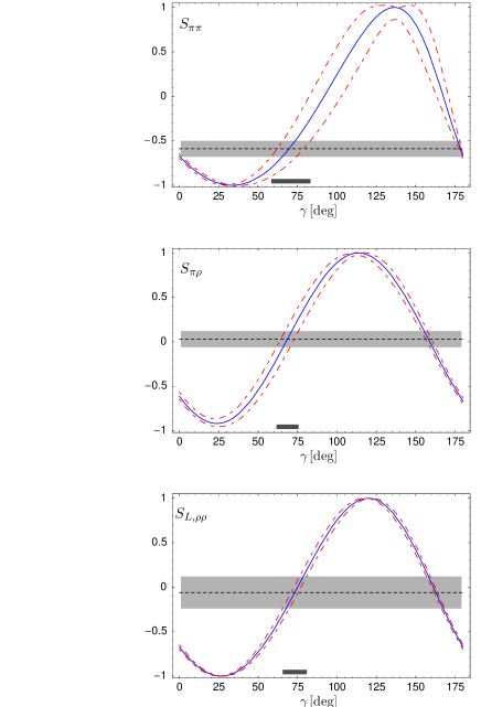
Figure 1: CKM phase $\gamma$ from $S_{f}$ with $f=(\pi\pi,\pi\rho,[\rho\rho]_{L})$.

6 DETERMINATION OF $\gamma$ FROM $S_{f}$

The time-dependent CP asymmetries $S_{f}$ in tree-dominated $\Delta D=1$ decays are particularly suited [19, 21] to determine the CKM phase $\gamma$ (or $\alpha$; I assume that $\beta$ is determined experimentally) in the framework of QCD factorization, since hadronic uncertainty enters only in the penguin correction; the dependence on strong phases is reduced, because it arises only through $\cos\delta$; the sensitivity to $\gamma$ is maximal near $\gamma\sim 70^{\circ}$.

Figure 1 shows that for $f=(\pi\pi,\pi\rho,[\rho\rho]_{L})$ and measurements $S_{f}=(-0.59\pm 0.09,0.03\pm 0.09,-0.06\pm 0.18)$ (HFAG averages), one obtains (ignoring a second solution that does not lead to consistent results) $\gamma=(70^{+13}_{-10},69\pm 7,73\pm 8)^{\circ}$. The three determinations are in agreement with each other, resulting in the average $\gamma=(71\pm 5)^{\circ}$. See [19, 29] for details.

7 CONCLUSION

The subject of hadronic decays has been and still is a very fertile ground for developing new theoretical concepts in heavy flavour physics. A lot has been learned about hadronic dynamics. Moreover, $\gamma$ is by now known rather well from charmless decays. There should be some way to include this information in the CKM fits.

References

- [1] D. Fakirov and B. Stech, Nucl. Phys. B 133 (1978) 315.
- [2] J. D. Bjorken, Nucl. Phys. Proc. Suppl. 11 (1989) 325.
- [3] M. Beneke, G. Buchalla, M. Neubert and C. T. Sachrajda, Phys. Rev. Lett. 83, 1914 (1999) [hep-ph/9905312]; Nucl. Phys. B 591, 313 (2000) [hep-ph/0006124].
- [4] J. Chay and C. Kim, Nucl. Phys. B 680 (2004) 302 [hep-ph/0301262].
- [5] M. Beneke and T. Feldmann, Nucl. Phys. B 685 (2004) 249 [hep-ph/0311335].
- [6] C. W. Bauer, D. Pirjol, I. Z. Rothstein and I. W. Stewart, Phys. Rev. D 70 (2004) 054015 [hep-ph/0401188].
- [7] M. Beneke and M. Neubert, Nucl. Phys. B 651 (2003) 225 [hep-ph/0210085].
- [8] A. R. Williamson and J. Zupan, Phys. Rev. D 74 (2006) 014003 [hep-ph/0601214].
- [9] Y. Y. Keum, H. N. Li and A. I. Sanda, Phys. Rev. D 63 (2001) 054008 [hep-ph/0004173].
- [10] M. Ciuchini, et al., Phys. Lett. B 515 (2001) 33 [hep-ph/0104126].
- [11] M. Beneke, G. Buchalla, M. Neubert and C. T. Sachrajda, Phys. Rev. D 72 (2005) 098501 [hep-ph/0411171]; M. Beneke, Int. J. Mod. Phys. A 21 (2006) 642 [hep-ph/0509297].
- [12] R. J. Hill, T. Becher, S. J. Lee and M. Neubert, JHEP 0407 (2004) 081 [hep-ph/0404217]; T. Becher and R. J. Hill, JHEP 0410 (2004) 055 [hep-ph/0408344].
- [13] G. G. Kirilin, [hep-ph/0508235].
- [14] M. Beneke and D. Yang, Nucl. Phys. B 736 (2006) 34 [hep-ph/0508250].
- [15] M. Beneke and S. Jäger, Nucl. Phys. B 751 (2006) 160 [hep-ph/0512351].
- [16] N. Kivel, [hep-ph/0608291].
- [17] M. Beneke and S. Jäger, hep-ph/0610322.
- [18] X. q. Li and Y. d. Yang, Phys. Rev. D 72 (2005) 074007 [hep-ph/0508079].
- [19] M. Beneke and M. Neubert, Nucl. Phys. B 675, 333 (2003), [hep-ph/0308039].
- [20] H. n. Li, S. Mishima and A. I. Sanda, Phys. Rev. D 72 (2005) 114005 [hep-ph/0508041].
- [21] M. Beneke, G. Buchalla, M. Neubert and C. T. Sachrajda, Nucl. Phys. B 606 (2001) 245 [hep-ph/0104110].
- [22] A. Khodjamirian, T. Mannel, M. Melcher and B. Melic, Phys. Rev. D 72, 094012 (2005) [hep-ph/0509049].
- [23] T. Feldmann and T. Hurth, JHEP 0411, 037 (2004) [hep-ph/0408188].
- [24] T. Becher, R. J. Hill, B. O. Lange and M. Neubert, Phys. Rev. D 69, 034013 (2004) [hep-ph/0309227]; T. Becher, R. J. Hill and M. Neubert, Phys. Rev. D 69, 054017 (2004) [hep-ph/0308122].
- [25] A. V. Manohar and I. W. Stewart, [hep-ph/0605001].
- [26] C. M. Arnesen, Z. Ligeti, I. Z. Rothstein and I. W. Stewart, [hep-ph/0607001].
- [27] A. L. Kagan, Phys. Lett. B 601 (2004) 151 [hep-ph/0405134].
- [28] M. Beneke, J. Rohrer and D. Yang, Phys. Rev. Lett. 96 (2006) 141801 [hep-ph/0512258].
- [29] M. Beneke, J. Rohrer and D. Yang, [hep-ph/0612290].
- [30] H. n. Li and S. Mishima, Phys. Rev. D 74 (2006) 094020 [hep-ph/0608277].
- [31] C. W. Bauer, I. Z. Rothstein and I. W. Stewart, Phys. Rev. D 74 (2006) 034010 [hep-ph/0510241].