KEK-TH-1129,

LYCEN 2006-23,

hep-ph/0612327

Lepton flavour violation in The Little Higgs model
S. Rai Choudhury¹ , A. S. Cornell² , A. Deandrea² , Naveen Gaur³ , A. Goyal⁴

¹ Center for Theoretical Physics, Jamia Millia University, Delhi - 110025, India,
² Université de Lyon 1, Institut de Physique Nucléaire,
4 rue E. Fermi, F-69622 Villeurbanne Cedex, France,
³ Theory Division, KEK, 1-1 Oho, Tsukuba, Ibaraki 305-0801, Japan
⁴ Dept. of Physics & Astrophysics, University of Delhi, Delhi - 110 007, India

Little Higgs models with T-parity have a new source of lepton flavour violation. In this paper we consider the anomalous magnetic moment of the muon $(g-2)_{\mu}$ and the lepton flavour violating decays $\mu\to e\gamma$ and $\tau\to\mu\gamma$ in Little Higgs model with T-parity [1]. Our results shows that present experimental constraints of $\mu\to e\gamma$ is much more useful to constrain the new sources of flavour violation which are present in T-parity models.

1 Introduction

Electroweak precision data suggests that the physics of electroweak symmetry breaking is weakly coupled, therefore, in order to have a natural theory, the Higgs mass needs to be protected from radiative corrections. As a means to solve this problem a number of extensions of the Standard Model (SM) have been proposed. In the effective theory approach the collective symmetry breaking mechanism of the Little Higgs (LH) models is an interesting possibility [2]. For earlier attempts to solve these issues see reference [3]. Note that a detailed review of LH models can be found in reference [4] (see also chapter 7 of reference [5]). Also, as the electroweak sector of the SM has been tested to a very high accuracy, an important test of the validity LH models through a comparison with precision data (for reviews treating this subject see references [6, 7]). Note that there exists many studies in the literature concerning the LH model and its implications to electroweak corrections (see for example reference [8]) and flavour physics both in hadronic [9] and leptonic sector [10].

The most serious constraints result from the tree-level corrections to precision electroweak observable due to the exchanges of the additional heavy gauge bosons present in the model, as well as from the small but non-vanishing vev of an additional weak-triplet scalar field. As a result, the fine-tuning of the Higgs boson mass is re-introduced. In order to forbid dangerous tree-level contributions to the electroweak observable, and avoid the appearance of a new fine tuning between the electroweak scale and the scale of the model, several new variants were proposed [11]. Particularly interesting is the implementation of a $Z_{2}$ symmetry called T-parity [12]. T-parity explicitly forbids tree-level contribution from the new heavy gauge bosons to the observable involving only SM particles as external states. It also forbids the interactions that induce triplet vev contributions. In T-parity symmetric LH models (LHT), corrections to precision electroweak observables are generated exclusively at loop level. Due to T-parity the lightest T-odd particle becomes stable. Since this lightest T-odd particle is electrically and colour neutral with ${\cal O}(100)$GeV it could be a candidate for dark matter [13, 14].

LHT predict heavy T-odd gauge bosons which are the T-partners of the SM gauge boson and also heavy T-odd $SU(2)$ doublet fermions. This structure is unique to LHT, and as the new particle masses can be relatively low, the next generation of colliders such as the Large Hadron Collider (LHC) has the great potential to directly produce the T-partners of the SM particles [15]. The peculiar structure of these models can also be tested using precision data, present and future colliders [16]. In particular the flavour structure of the model can be constrained both in the quark sector [17] and in the lepton sector.

The neutrino oscillation data from experiments is proving the existence of small neutrino mass and large neutrino flavour mixing. If the small neutrino mass as hinted by experiments is the only source of lepton flavour violation (LFV), then the LFV processes like $\mu\to e\gamma$ , $\tau\to\mu\mu\mu$ etc. would be heavily suppressed because of lepton sector GIM. The presence of new sources of LFV can enhance these processes to the level of present experimental limit. Little Higgs model with T-parity have a possible source of lepton flavour violation. In the following we shall concentrate on the mirror lepton sector, and on the interplay with the heavy T-odd gauge bosons sector of the Little Higgs model with T-parity, by studying the anomalous magnetic moment of the muon $(g-2)_{\mu}$ and the lepton family violating decays $\mu\to e\gamma$ and $\tau\to\mu\gamma$ , $\tau\to e\gamma$, $\tau\to\mu\mu\mu$, $\tau\to\mu M$ (semi-leptonic decay) etc..

2 Littlest Higgs model with T-parity

In this section we shall briefly review the Littlest Higgs model with T-parity of reference [12], in order to present our notation. We follow here, for the leptons, a notation similar to the one used by Buras et al.[17] in the analysis of non-minimal flavour violating interactions in the quark sector for LHT. Note that the model is a non-linear chiral-type Lagrangian based on the coset $SU(5)/SO(5)$.

The first stage of symmetry breaking is at a scale $f$ in the TeV range, and is due to the vacuum expectation value (vev) of an $SU(5)$ symmetric matrix $\Sigma$, that is:

$$\Sigma_{0}=\left(\begin{array}[]{ccc}0&0&\leavevmode\hbox{\small 1\normalsize\kern-3.30002pt1}\\ 0&1&0\\ \leavevmode\hbox{\small 1\normalsize\kern-3.30002pt1}&0&0\end{array}\right),$$ (2.1)

where 11 is the $2\times 2$ identity matrix. This breaking simultaneously breaks the gauge group to an $SU(2)\times U(1)$ subgroup, which is identified with the SM group. The origin of this symmetry breaking is not specified in the model but merely imposed. Therefore LHT are effective theories, valid up to a scale $\Lambda\sim 4\pi f$, as can be established in analogy with similar arguments in chiral Lagrangians. The generators, $T^{a}$, of the unbroken $SO(5)$ symmetry, are those which satisfy the relation $T^{a}\Sigma_{0}+\Sigma_{0}(T^{a})^{T}=0$. The broken generators, $X^{a}$, of $SU(5)/SO(5)$, satisfy the relation $X^{a}\Sigma_{0}-\Sigma_{0}(X^{a})^{T}=0$. The $SU(5)/SO(5)$ breaking gives rise to 14 Nambu-Goldstone bosons; four of the fourteen Goldstone bosons are absorbed by the broken gauge generators, and the remaining ten Goldstones are parameterized as:

$$\Pi=\left(\begin{array}[]{ccc}&h^{\dagger}/\sqrt{2}&\Phi^{\dagger}\\ h/\sqrt{2}&&h^{*}/\sqrt{2}\\ \Phi&h^{T}/\sqrt{2}&\end{array}\right),$$ (2.2)

where $h$ is the SM Higgs doublet and $\Phi$ is a complex $SU(2)$ triplet:

$$\Phi=\left(\begin{array}[]{cc}\Phi^{++}&\Phi^{+}/\sqrt{2}\\ \Phi^{+}/\sqrt{2}&\Phi^{0}\end{array}\right).$$ (2.3)

The second stage of symmetry breaking takes place as in the SM via the usual Higgs mechanism, at a scale $v=256$ GeV.

The effective theory at low energy is described by a chiral-type Lagrangian with the appropriate gauging (a $[SU(2)\times U(1)]^{2}$ subgroup of the global $SU(5)$ symmetry is gauged). T-parity exchanges the two $SU(2)\times U(1)$ factors. The symmetric tensor describing the low energy theory is:

$$\Sigma=e^{i\Pi/f}\Sigma_{0}e^{i\Pi^{T}/f}=e^{2i\Pi/f}\Sigma_{0}=\Sigma_{0}+\frac{2i}{f}\Pi\Sigma_{0}+{\cal O}(1/f^{2})\;,$$ (2.4)

where $f$ is the scale of symmetry breaking we have just described; similar to $f_{\pi}$ in the case of chiral Lagrangians. The kinetic term for the $\Sigma$ field can be written as:

$${\cal{L}}_{kin}=\displaystyle\frac{f^{2}}{8}\mathrm{Tr}\left\{D_{\mu}\Sigma(D^{\mu}\Sigma)^{\dagger}\right\},$$ (2.5)

where

$$D_{\mu}\Sigma=\partial_{\mu}\Sigma-i\Sigma_{j}\left[g_{j}W_{j}^{a}(Q_{j}^{a}\Sigma+\Sigma Q_{j}^{aT})+g^{\prime}_{j}B_{j}(Y_{j}\Sigma+\Sigma Y_{j})\right].$$ (2.6)

In the above $j=1,2$, the $Q_{j}$ and $Y_{j}$ are the gauged generators, $B_{j}$ and $W_{j}^{a}$ are the $U(1)_{j}$ and $SU(2)_{j}$ gauge fields, respectively, and $g_{j}$ and $g^{\prime}_{j}$ are the corresponding coupling constants.

2.1 Gauge bosons sector

In the gauge boson sector the gauge boson eigenstates are identified as:

$$W^{a}_{L}=\frac{W^{a}_{1}+W^{a}_{2}}{\sqrt{2}}\,,\qquad B_{L}=\frac{B_{1}+B_{2}}{\sqrt{2}},$$ (2.7)

$$W^{a}_{H}=\frac{W^{a}_{1}-W^{a}_{2}}{\sqrt{2}}\,,\qquad B_{H}=\frac{B_{1}-B_{2}}{\sqrt{2}},$$ (2.8)

where $L$ refers to the light (and T-even) states and $H$ the heavy (and T-odd) states. The mass eigenstates are then given, at ${\cal{O}}(v^{2}/f^{2})$, by the following combinations of gauge boson eigenstates:

$$W^{\pm}_{L} = \frac{W^{1}_{L}\mp iW^{2}_{L}}{\sqrt{2}}\,,\qquad Z_{L}=\cos\theta_{W}W^{3}_{L}-\sin\theta_{W}B_{L}\,,\qquad A_{L}=\sin\theta_{W}W^{3}_{L}+\cos\theta_{W}B_{L}\,,$$ (2.9)

$$W^{\pm}_{H} = \frac{W^{1}_{H}\mp iW^{2}_{H}}{\sqrt{2}}\,,\qquad Z_{H}=W^{3}_{H}+x_{H}\frac{v^{2}}{f^{2}}B_{H}\,,\qquad A_{H}=-x_{H}\frac{v^{2}}{f^{2}}W^{3}_{H}+B_{H}\,,$$ (2.10)

where $\theta_{W}$ is the weak mixing angle and $x_{H}=5gg^{\prime}/4(5g^{2}-g^{\prime 2})$ with $g$ and $g^{\prime}$ being, respectively, the $SU(2)$ and $U(1)$ gauge couplings. The gauge boson masses are then given at ${\cal{O}}(v^{2}/f^{2})$ by:

$$M_{W_{H}}=fg\left(1-\frac{v^{2}}{8f^{2}}\right),\qquad M_{Z_{H}}\equiv M_{W_{H}}\,,\qquad M_{A_{H}}=\frac{fg^{\prime}}{\sqrt{5}}\left(1-\frac{5v^{2}}{8f^{2}}\right).$$ (2.11)

The masses of the T-even gauge bosons are zero after the first stage of symmetry breaking and obtain a mass only through the second breaking, their masses being:

$$M_{W_{L}}=\frac{gv}{2}\left(1-\frac{v^{2}}{12f^{2}}\right),\quad M_{Z_{L}}=\frac{gv}{2\cos\theta_{W}}\left(1-\frac{v^{2}}{12f^{2}}\right),\quad M_{A_{L}}=0\,.$$ (2.12)

2.2 Mirror fermion sector and mixing

For each SM $SU(2)_{L}$ doublet, a doublet under $SU(2)_{1}$ and another under $SU(2)_{2}$ are introduced. The T-parity even linear combination is associated with the SM $SU(2)_{L}$ doublet, while the T-odd combination is given a mass of order of the scale $f$. This is required for a consistent implementation of T-parity in the fermion sector [12]. The fermion doublets are embedded into the following incomplete representations of $SU(5)$, and introduce a right-handed $SO(5)$ multiplet $\Psi_{R}$:

$$\Psi_{1}=\left(\begin{array}[]{c}i\psi_{1}\\ 0\\ 0\end{array}\right),\qquad\Psi_{2}=\left(\begin{array}[]{c}0\\ 0\\ i\psi_{2}\end{array}\right),\qquad\Psi_{R}=\left(\begin{array}[]{c}\tilde{\psi}_{R}\\ \chi_{R}\\ \psi_{R}\end{array}\right),$$ (2.13)

with

$$\psi_{i}=-\sigma^{2}f_{i}=-\sigma^{2}\pmatrix{u}_{i}\\ d_{i}\,,\qquad\psi_{R}=-i\sigma^{2}\pmatrix{u}_{HR}\\ d_{HR}$$ (2.14)

and $(i=1,2)$. Under T-parity these fields transform in the following way:

$$\Psi_{1}\mapsto-\Sigma_{0}\Psi_{2}\,,\qquad\Psi_{2}\mapsto-\Sigma_{0}\Psi_{1}\,,\qquad\Psi_{R}\mapsto-\Psi_{R}\,,$$ (2.15)

and the T-parity eigenstates of the fermion doublets are:

$$f_{L}=\frac{f_{1}-f_{2}}{\sqrt{2}}\,,\qquad f_{H}=\frac{f_{1}+f_{2}}{\sqrt{2}}\,.$$ (2.16)

$f_{L}$ are the left-handed SM fermion doublets (T-even), and $f_{H}$ are the left-handed mirror fermion doublets (T-odd). The right-handed mirror fermion doublet is given by $\psi_{R}$. The mirror fermions obtain a mass of the order of the scale $f$ [15]:

$$m^{d}_{Hi} = \sqrt{2}\kappa_{i}f\equiv m_{Hi},$$ (2.17)

$$m^{u}_{Hi} = \sqrt{2}\kappa_{i}f\left(1-\frac{v^{2}}{8f^{2}}\right)=m_{Hi}\left(1-\frac{v^{2}}{8f^{2}}\right)\,,$$ (2.18)

where $\kappa_{i}$ are the eigenvalues of the mass matrix $\kappa$. The additional fermions $\tilde{\psi}_{R}$ and $\chi_{R}$ can be given large Dirac masses, and we assume that they are decoupled from the theory.

In a similar way to what happens for standard fermions, the mirror sector has weak mixing, parameterised by unitary mixing matrices; two for mirror leptons and two for mirror quarks:

$$V_{H\ell}\,,\quad V_{H\nu}\,,\quad V_{Hu}\,,\quad V_{Hd}\,,$$ (2.19)

which satisfy the following physical constraints:

$$V_{H\nu}^{\dagger}V_{H\ell}=V_{PMNS}\,,\qquad V_{Hu}^{\dagger}V_{Hd}=V_{CKM}\,.$$ (2.20)

Furthermore, this implies that one can not turn off the new mixing effects, except with a universal degenerate mass spectrum for the T-odd doublets. In the following we shall set the Majorana phases of $V_{PMNS}$ to zero, as no Majorana mass term has been introduced for the right-handed neutrinos. The mixing in the lepton sector will be the main focus of our phenomenological analysis. Note that a detailed discussion of the parameterisation of the mirror lepton mixing matrices is given in section IV.

3 Analytical results of $(g-2)_{\mu}$ and $\mu\to e\gamma$

In this section we shall summarize our analytic results for the anomalous magnetic moment of the muon $(g-2)_{\mu}$ and the two lepton family violating decays $\mu\to e\gamma$ and $\tau\to\mu\gamma$ from the Littlest Higgs model with T-parity.

3.1 Anomalous magnetic moment of the muon

For the $(g-2)_{\mu}$ in LHT we have the following additional contributions:

• The $W^{\pm}_{H}$ contribution.

• The $Z_{H}$ contribution

• The $A_{H}$ contribution.

• And the $\Phi$ (triplet Higgs) contribution.

As such, the additional diagrams which will contribute to $(g-2)_{\mu}$ (at one loop level) are given in Fig (1), and where the contribution to the $a_{\mu}$ due to the new particles can be written as:

$$a_{\mu}^{LH}=a_{\mu}(W_{H})+a_{\mu}(A_{H})+a_{\mu}(Z_{H})+a_{\mu}(\Phi).$$ (3.21)

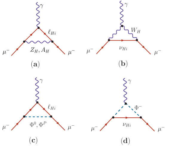
Figure 1: Diagrams of the additional contributions to the $(g-2)_{\mu}$ arising from LHT

Note that the contributions due to triplet Higgs ($\Phi$) can be neglected, as their coupling to SM fermions and T-odd fermions is of order $(v/f)^{2}$ (see Appendix A of reference [17]). As such, the diagrams Fig (1 c), and (1 d) will give contributions at the $(v/f)^{4}$ level (as these diagrams have two vertices involving the triplet Higgs). In order $(v/f)^{2}$ calculations we can therefore neglect any such contributions. This means we shall only consider contributions due to heavy gauge bosons given by diagrams Fig (1 a) and (1 b).

The various contributions due to gauge bosons in the unitary gauge are:

$$a_{\mu}(W_{H}) = -\frac{g^{2}}{32\pi^{2}}\frac{m_{\mu}^{2}}{M_{W_{H}}^{2}}\sum_{i=1,3}\left(V_{H\nu}\right)_{2i}^{*}\left(V_{H\nu}\right)_{2i}F_{W_{H}}(x_{i})\quad,\quad\mathrm{where}\quad x_{i}=\left(\frac{M_{\nu_{H_{i}}}}{M_{W_{H}}}\right)^{2},$$ (3.22)

$$a_{\mu}(Z_{H}) = \frac{g^{2}}{32\pi^{2}}\frac{m_{\mu}^{2}}{M_{Z_{H}}^{2}}\sum_{i=1,3}\left(V_{H\ell}\right)_{2i}^{*}\left(V_{H\ell}\right)_{2i}F_{Z_{H}}(y_{i})\quad,\quad\mathrm{where}\quad y_{i}=\left(\frac{M_{\ell_{H_{i}}}}{M_{Z_{H}}}\right)^{2},$$ (3.23)

$$a_{\mu}(A_{H}) = \frac{g^{\prime 2}}{800\pi^{2}}\frac{m_{\mu}^{2}}{M_{A_{H}}^{2}}\sum_{i=1,3}\left(V_{H\ell}\right)_{2i}^{*}\left(V_{H\ell}\right)_{2i}F_{Z_{H}}(z_{i})\quad,\quad\mathrm{where}\quad z_{i}=\left(\frac{M_{\ell_{H_{i}}}}{M_{A_{H}}}\right)^{2},$$ (3.24)

and where the functions $F_{X}(x)$ have been defined in Appendix B.

In the next section we shall generate plots of $a_{\mu}^{LH}$ for various values of $f$ and mirror lepton masses.

3.2 Lepton family violating decays

We shall now consider the lepton family violating decays of the form $f_{1}(p_{1})\to f_{2}(p_{2})\gamma(q)$, with $q=p_{1}-p_{2}$. In these calculations we shall take the fermions $f_{1}$ and $f_{2}$ as having masses $m_{1}$ and $m_{2}$ respectively. As the external fermions are on mass shell, we also have that $p_{1}^{2}=m_{1}^{2}$, $p_{2}^{2}=m_{2}^{2}$. As such, the amplitude for the decay can can be written as $e\epsilon_{\mu}^{*}(q){\cal M}^{\mu}$, where $\epsilon_{\mu}^{*}(q)$ is the polarization vector of the emitted photon. The most general ${\cal M}^{\mu}$ for an on-shell photon can be written as [18]:

$${\cal M}^{\mu}=i\bar{u}_{2}\left[\sigma^{\mu\nu}q_{\nu}\left(\sigma_{L}P_{L}+\sigma_{R}P_{R}\right)\right]u_{1},$$ (3.25)

where $P_{L}=(1-\gamma_{5})/2$, $P_{R}=(1+\gamma_{5})/2$ and $\sigma_{L}$, $\sigma_{R}$ are the respective coefficients. From the expression given in equation (3.25) we get the partial decay width for $f_{1}\to f_{2}\gamma$ as:

$$\Gamma=\frac{\left(m_{1}^{2}-m_{2}^{2}\right)^{3}}{16\pi m_{1}^{3}}\left(|\sigma_{L}|^{2}+|\sigma_{R}|^{2}\right).$$ (3.26)

Assuming the fermions $f_{1}$ and $f_{2}$ interact with a neutral or charged vector boson, $B_{\alpha}$, and with another fermion $F$, the gauge interaction part of the Langrangian can be written as:

$${\cal L}=\sum_{i=1}^{2}\left[B_{\mu}\bar{F}\gamma^{\mu}\left(L_{i}P_{L}+R_{i}P_{R}\right)f_{i}+B_{\mu}^{*}\bar{f}_{i}\gamma^{\mu}\left(L_{i}^{*}P_{L}+R^{*}_{i}P_{R}\right)F\right],$$ (3.27)

where $L_{i}$ and $R_{i}$ are coefficients of the operators (model dependent). In our case (LHT), from Table 1 in Appendix A, we can see that we do not have any right-handed currents contributing to the process. As such, $R_{i}=0$. Equation (3.27) then becomes, for our case:

$${\cal L}=\sum_{i=1}^{2}\left[B_{\mu}\bar{F}\gamma^{\mu}L_{i}P_{L}f_{i}+B_{\mu}^{*}\bar{f}_{i}\gamma^{\mu}L^{*}_{i}P_{L}F\right].$$ (3.28)

Note that we shall again assume that the Higgs exchange diagrams will not contribute, as they are higher order in $(v/f)^{2}$.

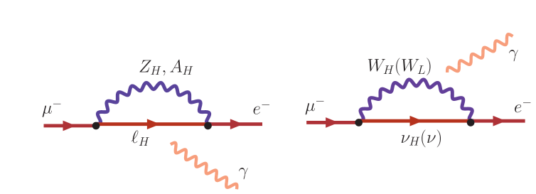
Figure 2: The Feynman diagrams for $\mu\to e\gamma$ in LHT

In the LH model we will also have contributions from loops containing mirror fermions, $W_{H},Z_{H}$ and $A_{H}$. Their contributions to $\sigma_{L}$ and $\sigma_{R}$ (as defined in equation (3.25)) can be defined as:

$$\sigma_{L}=(\sigma_{L})_{W_{H}}+(\sigma_{L})_{Z_{H}}+(\sigma_{L})_{A_{H}},$$

$$\sigma_{R}=(\sigma_{R})_{W_{H}}+(\sigma_{R})_{Z_{H}}+(\sigma_{R})_{A_{H}}.$$ (3.29)

Where the expressions for the $\sigma$’s above are given in Appendix C. However, as one final note, in our case (with T-parity) equation (3.27) can be expressed as, using the vertices given in Table 1:

$${\cal L} = \frac{ig}{\sqrt{2}}\sum_{ij}\bar{\nu}_{H_{i}}\gamma_{\mu}P_{L}(V_{H\ell})_{ij}\ell_{j}W_{H}^{\mu}+i\left(-\frac{g}{\sqrt{2}}+\frac{g^{\prime}}{10}x_{H}\frac{v^{2}}{f^{2}}\right)\sum_{ij}\bar{\ell}_{H_{i}}\gamma_{\mu}P_{L}(V_{H\ell})_{ij}\ell_{j}Z_{H}^{\mu}$$ (3.30)

$$+i\left(\frac{g^{\prime}}{10}+\frac{g^{\prime}}{10}x_{H}\frac{v^{2}}{f^{2}}\right)\sum_{ij}\bar{\ell}_{H_{i}}\gamma_{\mu}P_{L}(V_{H\ell})_{ij}\ell_{j}A_{H}^{\mu}+{\cal O}\left(\frac{v^{4}}{f^{4}}\right).$$

In the next section we shall study how the branching ratios for the decays $\mu\to e\gamma$ and $\tau\to\mu\gamma$ change for different values of the parameter $f$, and for various mirror lepton masses.

4 Numerical Analysis & Discussion

For our numerical results we shall use the standard parameterisation the of $V_{PMNS}$ matrix, which can be written as:

$$V_{PMNS} = \left(\begin{array}[]{c c c}1&0&0\\ 0&c_{atm}&s_{atm}\\ 0&-s_{atm}&c_{atm}\end{array}\right)\left(\begin{array}[]{c c c}c_{rct}&0&s_{rct}e^{-i\delta_{r}}\\ 0&1&0\\ -s_{rct}e^{i\delta_{r}}&0&c_{rct}\end{array}\right)\left(\begin{array}[]{c c c}c_{sol}&s_{sol}&0\\ -s_{sol}&c_{sol}&0\\ 0&0&1\end{array}\right)$$

$$= U(\theta_{atm})U(\theta_{rct})U(\theta_{sol}),$$

where the $\theta_{atm}$, $\theta_{rct}$ and $\theta_{sol}$ are the atmospheric, reactor and solar mixing angles. From neutrino oscillation experiments we have $\triangle m_{12}^{2}\sim 8\times 10^{-5}{\rm eV^{-2}}$, $sin^{2}2\theta_{sol}\sim 0.31$, $|\triangle m_{13}^{2}|\sim 2.6\times 10^{-3}{\rm eV^{2}}$, $sin^{2}2\theta_{atm}\sim 1.0$ and $sin\theta_{rct}\leq 0.2$ (for our calculations we have taken $\sin\theta_{rct}=0.2$). From WMAP constraints we also have that $\sum_{i=1,2,3}m_{i}<2eV$ (that is, the sum of the masses of the three SM neutrino species). As such, the structure of the leptonic sector mixing matrix, $V_{PMNS}$, which is analogous to the quark sector CKM matrix, can give rise to the lepton flavour violating processes (such as $\mu\to e\gamma$ , $\tau\to\mu\gamma$ , $\tau\to\mu(\pi,K)$, $\tau^{-}\to\mu^{-}(e^{-})\mu^{+}\mu^{-}$ etc.) within the SM. Where, to reiterate, these flavour violating processes, within the SM, will be dependent upon the structure of the mixing matrix ($V_{PMNS}$) and the neutrino masses. Note that the smallness of neutrino mass, as indicated by WMAP data, ensures the suppression of these processes to a level which cannot be probed even in foreseeable future. Furthermore, the lepton sector GIM mechanism suppresses the branching ratio of $\mu\to e\gamma$ to a value less than $10^{-40}$ within the SM. As such, we shall refer to this situation as Minimal Flavour Violation (MFV).

As discussed earlier, in LHT we can have a new mechanism for lepton flavour violation, where, in the T-parity model the LFV can come from the flavour mixing in the mirror fermion sector. The mixing in that mirror fermion sector can, furthermore, give rise to a TeV scale GIM mechanism. Note that this has been extensively discussed in the case of hadronic decays [17]. The possible implications of this TeV scale GIM mechanism, in the case of lepton sector, has been stressed in the T-parity model [1]. There is a possibility of large enhancement of LFV decays in the T-parity model, despite the presence of a TeV scale GIM mechanism in the lepton sector. As such, we shall quantify this by calculating some definite values of the mixing matrix and other LH parameters.

The new mixing matrix which gives rise to flavour violation in the lepton sector ($V_{H\ell}$), in general, has four parameters; namely three angles and one phase. The presence of this mixing matrix arises from the possibility of a departure from MFV, which was present within the SM. We therefore parameterise this mixing matrix with three mixing angles ($\theta_{12},\theta_{23},\theta_{13}$) and a phase ($\delta$) as:

$$V_{H\ell} = \left(\begin{array}[]{c c c}1&0&0\\ 0&c_{23}&s_{23}\\ 0&-s_{23}&c_{23}\end{array}\right)\left(\begin{array}[]{c c c}c_{13}&0&s_{13}e^{-i\delta}\\ 0&1&0\\ -s_{13}e^{i\delta}&0&c_{13}\end{array}\right)\left(\begin{array}[]{c c c}c_{12}&s_{12}&0\\ -s_{12}&c_{12}&0\\ 0&0&1\end{array}\right)$$

$$= U(\theta_{23})U(\theta_{13})U(\theta_{12}).$$

At this point we would like to stress that for the departure from MFV, within the SM, the following conditions need to be satisfied:

1. The matrix $V_{H\ell}$ should be different from the Identity matrix.

2. And that the three generations of mirror fermions should not be degenerate in mass.

From the above structural considerations of the mixing matrices, where as a benchmark we will show the results of LFV processes for the following cases:

1. Case A: Where we assume that $V_{H\ell}$ is related to $V_{PMNS}$, such that no additional new parameters, except those of the masses of mirror fermions, will be needed.

2. Case B: Where we assume the hierarchy of the mixing angles to be:

   $$s_{12}\ll s_{13}\ll s_{23}.$$ (4.51)

3. Case C: And finally, where we assume that the hierarchy of the mixing angles is:

   $$s_{12}\ll s_{23}\ll s_{13}.$$ (4.52)

We shall now analyze the effects of the above cases on our observables for $(g-2)_{\mu}$ , $\mu\to e\gamma$ and $\tau\to\mu\gamma$ , where the present experimental bounds for the observables are[20]:

$$\delta a_{\mu} = 22(10)\times 10^{-10},$$

$$Br(\mu\to e\gamma) \leq 1.2\times 10^{-11}\quad[90\%\ C.L.],$$

$$Br(\tau\to\mu\gamma) \leq 6.8\times 10^{-8}\quad[90\%\ C.L.].$$

Firstly, we shall present the results for $\delta a_{\mu}$ in the case where the mirror leptons have degenerate mass. In this case we only have two parameters in the model, namely; the LH scale ($f$) and mass of the mirror leptons. The results are plotted in Fig (3). As mentioned above, this is the MFV case of the SM, and hence $\mu\to e\gamma$ and $\tau\to\mu\gamma$ will stay at their SM levels. Note that, as we can be observed from the graph, although $\delta a_{\mu}$ shows substantial variation as a function of the LH scale, its value is still much lower than the present experimental bounds.

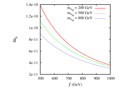
Figure 3: $\delta a_{\mu}$, where we have assumed $m_{\ell_{H}}=m_{\nu_{H}}$, i.e. the same mass for all the mirror fermion doublets

4.1 Case A

In this case we shall consider $V_{H\ell}$ as being related to $V_{PMNS}$. In this case we do not introduce any additional parameters, except the masses of the mirror fermions. For $V_{PMNS}$ we take the standard parameterisation with parameters given by the neutrino experiments. Furthermore, we shall discuss the four cases, in analogy to the discussion given in reference [19], namely:

1. : $V_{H\ell}=V_{PMNS}$ .

2. : $V_{H\ell}=U(\theta_{atm})U(\theta_{rct})$ .

3. : $V_{H\ell}=U(\theta_{atm})$ .

4. : $V_{H\ell}=I$ .

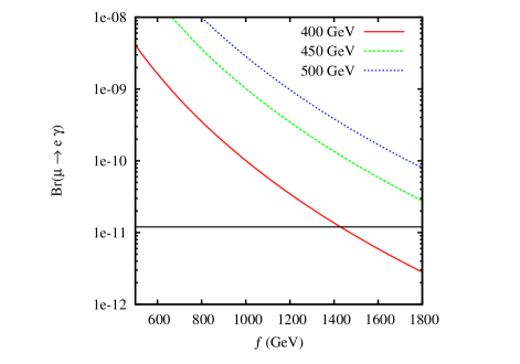
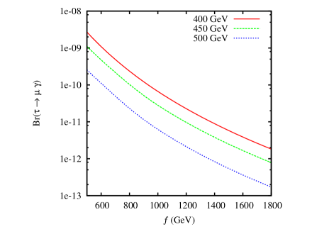
Figure 4: Case A - I ($V_{H\ell}=V_{PMNS}$): $\mu\to e\gamma$ ($\tau\to\mu\gamma$ ) as a function of $f$ in the left (right) panel for different values of the second generation mirror lepton mass. The masses of first and third generation mirror leptons are 400 GeV and 500 GeV respectively.

Case A - I : We have presented our results of case I in Fig (4). As can be seen from the figure, in this case the branching ratios are very sensitive to the mass splitting of the mirror leptons. Furthermore, in this case the experimental measurement of $\mu\to e\gamma$ practically rules out any substantial mass splitting between all three generations of the mirror leptons. For this case we have also shown a scatter plot of the correlation between $\mu\to e\gamma$ and $\tau\to\mu\gamma$ in Fig (7). In this plot we have varied the masses of the mirror leptons in the range 500-600 GeV. As can be seen from this figure, the $\mu\to e\gamma$ decay practically rules out most of the region where there is splitting between the mirror lepton masses. However, there are still some regions where we can have a fairly high (although still within the experimental limits) rate for the $\tau\to\mu\gamma$ decay. Note that any improvement in the $\tau\to\mu\gamma$ decay rate in the future would further constrain these parameters.

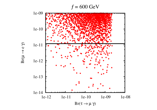
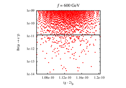
Figure 5: Case A Co-relation between the $\tau\to\mu\gamma$ and $\mu\to e\gamma$ decays (left panel) and the $\mu\to e\gamma$ and $(g-2)_{\mu}$ (right panel). Masses of the heavy (mirror) leptons are varied randomly in the range $500<m_{\ell_{H}}<700$ GeV and $f=600$ GeV.

Case A - II & III : In these cases there is no significant change in the rate of the $\mu\to e\gamma$ decay for the range of mirror lepton masses considered here. The reason for this is due to these cases corresponding to the the situation where $V_{H\ell}=V_{PMNS}$, and $s_{12}=0$ for case II, and $s_{12}=s_{13}=0$ for case III. In this case we do not have any appreciable mixing in the first two generations of the mirror leptons, and hence no great change in the predictions of the $\mu\to e\gamma$ decay. However, the rate of the $\tau\to\mu\gamma$ decay can be substantially changed. We have plotted the rate of the $\tau\to\mu\gamma$ decay as a function of LH scale for case II and III in Fig (6). As can be seen from these plots in Fig (6), the predictions are still below the present experimental bounds. However, if data for the $\tau\to\mu\gamma$ decay were improved in future, from high luminosity SuperB factories, this would help to constrain the possibilities greatly.

Case A - IV : This is the MFV limit of the LHT model. In this case as there is no mixing in mirror lepton sector hence there will not be any contribution to LFV processes.

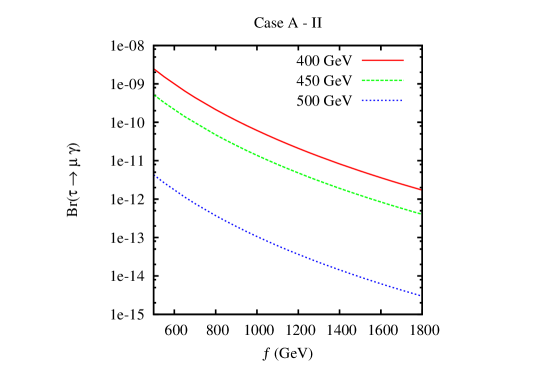
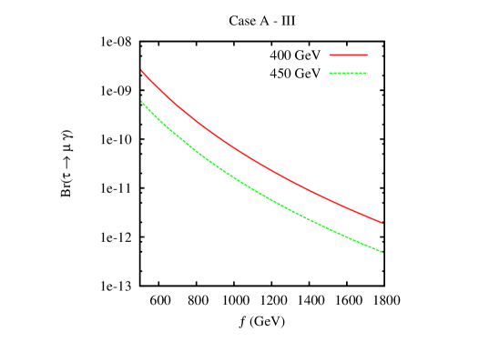
Figure 6: Case A - II (left panel), III (right panel): The $\tau\to\mu\gamma$ decay as a function of $f$ for different values of the second generation mirror lepton mass. The masses of the first and third generation of the mirror leptons are 400 GeV and 500 GeV respectively.

4.2 Case B

In this case we have assumed the pattern $s_{12}\ll s_{13}\ll s_{23}$. In Fig (7) we have shown the results for the fixed values of the angles, as given by:

$$s_{23}\sim 0.2,~{}~{}s_{13}\sim 0.02,~{}~{}s_{12}\sim 0.002.$$

This pattern assures a very small mixing in the first two generations of the mirror leptons, which ensures we keep the $\mu\to e\gamma$ decay rate rather low. However, in this case we can still have sufficient mixing in the second and third generations to have a higher rate (although still within the present experimental bounds) for the $\tau\to\mu\gamma$ decay.

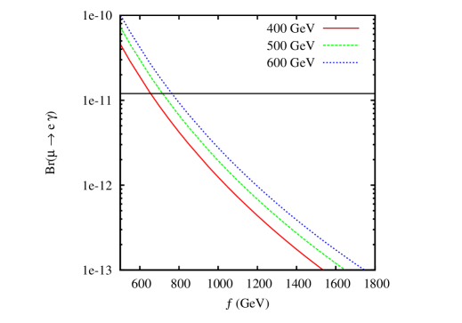
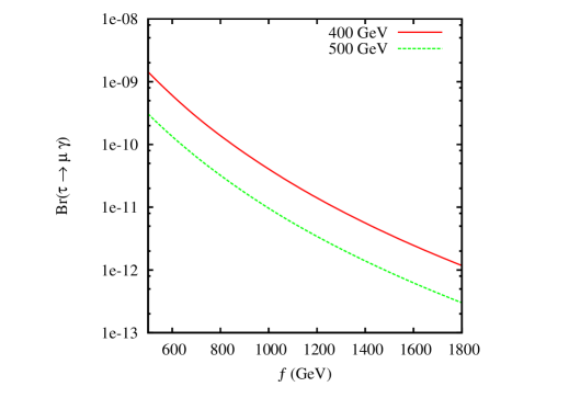
Figure 7: Case B: The $\mu\to e\gamma$ ($\tau\to\mu\gamma$ ) decay as a function of $f$, in the left (right) panel, for different values of the second generation mirror lepton mass. The masses of the first and third generation of mirror leptons are 400 GeV and 600 GeV respectively.

4.3 Case C

In this case we are assuming a hierarchy $s_{12}\ll s_{23}\ll s_{13}$, where in Fig (8) we have plotted for specific values of the angles, given by:

$$s_{23}\sim 0.02,\quad s_{13}\sim 0.2,\quad s_{12}\sim 0.002.$$

In this case the mixing matrix $V_{H\ell}$ is essentially diagonal. As such there is very little mixing between the mirror leptons, which results in a lower value for the decay rates of $\mu\to e\gamma$ and $\tau\to\mu\gamma$ .

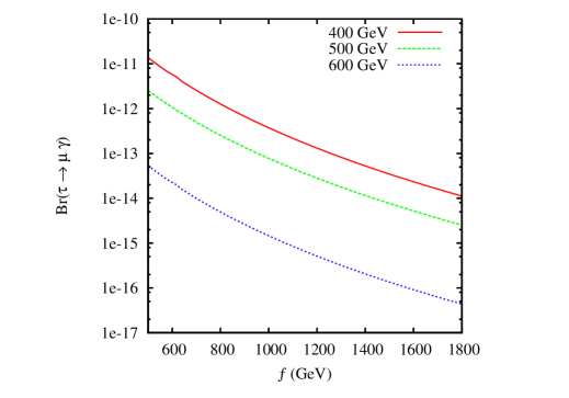
Figure 8: Case C: The $\mu\to e\gamma$ ($\tau\to\mu\gamma$ ) decay as a function of $f$, in the left (right) panel, for different values of the second generation mirror lepton mass. The masses of the first and third generation of mirror leptons are 400 GeV and 600 GeV respectively.

To summarize, the precision constraints on the anomalous magnetic moment of muon ($\delta a_{\mu}$) does not constrain the LHT. However, as T-parity models have new source of lepton flavour violation one can extract useful constraints on model parameters from various lepton flavour violating processes. In this paper we have analyzed the effects of these new flavour violations in T-parity models on the decays $\mu\to e\gamma$ and $\tau\to\mu\gamma$ . From the experimental results of the $\mu\to e\gamma$ decay, rather strong constraints on the texture of the new flavour violating mixing matrix, and the mass splitting of mirror leptons is given. Note that there are practically no constraints from the $\tau\to\mu\gamma$ decay on the model parameters from present experimental results, however, the future SuperB factories, which may observe the $\tau\to\mu\gamma$ and $\tau\to e\gamma$ decays at rates of $10^{-10}$, might provide us very useful constraints on the model parameters.

Appendix A Feynman Rules

In this appendix we list all the relevant Feynman rules for our analysis, which have been summarized in Table 1 [17].

Particles	Vertices	Particles	Vertices
$\bar{\ell}_{i}W_{L}^{-\mu}\nu_{j}$	$i\frac{g}{\sqrt{2}}\left(V_{PMNS}\right)_{ij}P_{L}$	$\bar{\nu}_{H_{i}}W_{H}^{+\mu}\ell_{j}$	$i\frac{g}{\sqrt{2}}\left(V_{H\ell}\right)_{ij}P_{L}$
$\bar{\ell}_{i}Z_{L}^{\mu}\ell_{j}$	$\frac{ig}{cos\theta_{w}}\gamma^{\mu}\left[\left(-{1\over 2}+sin^{2}\theta_{w}\right)P_{L}+sin^{2}\theta_{w}P_{R}\right]\delta_{ij}$	$\bar{\ell}_{H_{i}}Z_{H}^{\mu}\ell_{j}$	$i\left(-\frac{g}{2}+\frac{g^{\prime}}{10}x_{H}\frac{v^{2}}{f^{2}}\right)\left(V_{H_{\ell}}\right)_{ij}\gamma^{\mu}P_{L}$
$\bar{\ell}_{i}A_{L}^{\mu}\ell_{j}$	$-ig^{\prime}\gamma^{\mu}\delta_{ij}$	$\bar{\ell}_{H_{i}}A_{H}^{\mu}\ell_{j}$	$i\left(\frac{g^{\prime}}{10}+\frac{g^{\prime}}{10}x_{H}\frac{v^{2}}{f^{2}}\right)\left(V_{H_{\ell}}\right)_{ij}\gamma^{\mu}P_{L}$

Table 1: where $x_{H}=\frac{5gg^{\prime}}{4(5g^{2}-g^{\prime 2})}$. Vertices taken from Buras et al.[17]

Appendix B Functions for $(g-2)_{\mu}$

The functions used in the determination of the LH contribution to $(g-2)_{\mu}$ are [21]:

$$F_{W_{H}}(x_{i}) = \int^{1}_{0}dy\frac{-2y^{2}(1+y)-x_{i}(2y-3y^{2}+y^{3})-x_{\mu}y^{2}(y-1)}{y+x_{\mu}(y^{2}-y)+x_{i}(1-y)},$$ (B.53)

$$F_{Z_{H}}(y_{i}) = \int^{1}_{0}dx\frac{(x-x^{2})(x-2)-{1\over 2}\left(y_{i}(x^{3}+x^{2})+x_{\mu}(x^{3}-x^{2})\right)}{(1-x)+x_{\mu}(x^{2}-x)+y_{i}x},$$ (B.54)

with $x_{\mu}=\left(\frac{m_{\mu}}{M_{W_{H}}}\right)^{2}$.

In the limit $x_{\mu}\to 0$, that is, where we neglect the $\mu$ mass when compared to $M_{W_{L}}$, the above integrations can be analytically expressed as:

$$F_{W_{H}}(x_{i}) = -\frac{10-43x_{i}+78x_{i}^{2}-49x_{i}^{3}+4x_{i}^{4}+18x_{i}^{3}Log(x_{i})}{6\left(x_{i}-1\right)^{4}},$$ (B.55)

$$F_{Z_{H}}(y_{i}) = \frac{-8+38y_{i}-39y_{i}^{2}+14y_{i}^{3}-5y_{i}^{4}+18y_{i}^{2}Log(y_{i})}{12(y_{i}-1)^{4}}.$$ (B.56)

Appendix C Functions for $\mu\to e\gamma$ and $\tau\to\mu\gamma$

In determining the branching ratio for the decays $\mu\to e\gamma$ and $\tau\to\mu\gamma$ , we have made use of the following expressions [18]. Firstly note that apon comparing equation (3.28) with equation (3.29) for the $\mu\to e\gamma$ decay the coefficients $L_{i}$ will have values:

$$\begin{array}[]{l l l }W_{H}\ contribution:&(L_{\mu}^{W_{H}})^{*}_{i}=\frac{ig}{\sqrt{2}}\left(V_{H\ell}\right)_{2i},&(L_{e}^{W_{H}})^{*}_{i}$ = - $\frac{ig}{\sqrt{2}}\left(V_{H\ell}\right)^{*}_{i1}\\ Z_{H}\ contribution:&(L_{\mu}^{Z_{H}})_{i}=i\left(-\frac{g}{\sqrt{2}}+\frac{g^{\prime}}{10}x_{H}\frac{v^{2}}{f^{2}}\right)\left(V_{H\ell}\right)_{2i},&(L_{e}^{Z_{H}})^{*}_{i}=-i\left(-\frac{g}{\sqrt{2}}+\frac{g^{\prime}}{10}x_{H}\frac{v^{2}}{f^{2}}\right)\left(V_{H\ell}\right)^{*}_{i1}\\ A_{H}\ contribution:&(L_{\mu}^{A_{H}})_{i}=i\left(\frac{g^{\prime}}{10}+\frac{g^{\prime}}{10}x_{H}\frac{v^{2}}{f^{2}}\right)\left(V_{H\ell}\right)_{2i},&(L_{e}^{A_{H}})^{*}_{i}=-i\left(\frac{g^{\prime}}{10}+\frac{g^{\prime}}{10}x_{H}\frac{v^{2}}{f^{2}}\right)\left(V_{H\ell}\right)^{*}_{i1},\\ \end{array}$$ (C.57)

where the index $i$ sums over the three generation of mirror fermions, where analogous expressions for the decay $\tau\to\mu\gamma$ are given by selecting the appropriate elements in $V_{H\ell}$. Defining now the product:

$$\lambda^{X}_{i}=(L_{\mu}^{X})_{i}(L_{e}^{X})^{*}_{i},\quad X=W_{H},Z_{H},A_{H},$$ (C.58)

the LH contributions to $\sigma$, as defined in equation (3.29), can be written as:

$$\begin{array}[]{l l l}W_{H}\ loop:{}{}&(\sigma_{L})_{W_{H}}=Q_{W_{H}}\ \lambda^{W_{H}}_{i}\ \bar{y}_{2}(m_{\nu_{H}}^{i},m_{W_{H}}),{}{}{}&(\sigma_{R})_{W_{H}}=Q_{W_{H}}\ \lambda^{W_{H}}_{i}\ \bar{y}_{1}(m_{\nu_{H}}^{i},m_{W_{H}}),\\ Z_{H}\ loop:{}{}&(\sigma_{L})_{Z_{H}}=Q_{\ell_{H}}\ \lambda^{Z_{H}}_{i}\ y_{2}(m_{\ell_{H}}^{i},m_{Z_{H}}),{}{}{}&(\sigma_{R})_{Z_{H}}=Q_{\ell_{H}}~{}\lambda^{Z_{H}}_{i}\ y_{1}(m_{\ell_{H}}^{i},m_{Z_{H}}),\\ A_{H}\ loop:{}{}&(\sigma_{L})_{A_{H}}=Q_{\ell_{H}}\ \lambda^{A_{H}}_{i}\ y_{2}(m_{\ell_{H}}^{i},m_{A_{H}}),{}{}{}&(\sigma_{R})_{A_{H}}=Q_{\ell_{H}}~{}\lambda^{A_{H}}_{i}\ y_{1}(m_{\ell_{H}}^{i},m_{A_{H}}),\\ \end{array}$$ (C.59)

where $Q_{W_{H}}$ is the charge of $W_{H}$ and $Q_{\ell_{H}}$ is the charge of heavy mirror lepton. The loops and y functions are given as:

$$y_{1}(m_{F},m_{B}) = m_{1}\left[2a+4c_{1}+2c_{2}+2d_{1}+2f+\frac{m_{F}^{2}}{m_{B}^{2}}\left(-c_{2}+d_{1}+f\right)+\frac{m_{2}^{2}}{m_{B}^{2}}\left(c_{2}+d_{2}+f\right)\right],$$

$$y_{2}(m_{F},m_{B}) = m_{2}\left[2a+2c_{1}+4c_{2}+2d_{1}+2f+\frac{m_{F}^{2}}{m_{B}^{2}}\left(-c_{1}+d_{2}+f\right)+\frac{m_{1}^{2}}{m_{B}^{2}}\left(c_{1}+d_{1}+f\right)\right],$$

$$\bar{y}_{1}(m_{F},m_{B}) = m_{1}\left[2\bar{c}_{2}+2\bar{d}_{1}+2\bar{f}+\frac{m_{F}^{2}}{m_{B}^{2}}\left(\bar{a}-2\bar{c}_{1}-\bar{c}_{2}+\bar{d}_{1}+\bar{f}\right)+\frac{m_{2}^{2}}{m_{B}^{2}}\left(-\bar{c}_{2}+\bar{d}_{2}+\bar{f}\right)\right],$$

$$\bar{y}_{2}(m_{F},m_{B}) = m_{2}\left[2\bar{c}_{1}+2\bar{d}_{2}+2\bar{f}+\frac{m_{F}^{2}}{m_{B}^{2}}\left(\bar{a}-\bar{c}_{1}-2\bar{c}_{2}+\bar{d}_{2}+\bar{f}\right)+\frac{m_{1}^{2}}{m_{B}^{2}}\left(-\bar{c}_{1}+\bar{d}_{1}+\bar{f}\right)\right].$$ (C.60)

Where in the above equations we have used:

$$a = \frac{i}{16\pi^{2}}C_{0}(m_{1}^{2},q^{2},m_{2}^{2},m_{B}^{2},m_{F}^{2},m_{F}^{2}),$$

$$c_{1} = \frac{i}{16\pi^{2}}C_{1}(m_{1}^{2},q^{2},m_{2}^{2},m_{B}^{2},m_{F}^{2},m_{F}^{2}),$$

$$c_{2} = \frac{i}{16\pi^{2}}C_{2}(m_{1}^{2},q^{2},m_{2}^{2},m_{B}^{2},m_{F}^{2},m_{F}^{2}),$$

$$d_{1} = \frac{i}{16\pi^{2}}C_{11}(m_{1}^{2},q^{2},m_{2}^{2},m_{B}^{2},m_{F}^{2},m_{F}^{2}),$$

$$d_{2} = \frac{i}{16\pi^{2}}C_{22}(m_{1}^{2},q^{2},m_{2}^{2},m_{B}^{2},m_{F}^{2},m_{F}^{2}),$$

$$f = \frac{i}{16\pi^{2}}C_{12}(m_{1}^{2},q^{2},m_{2}^{2},m_{B}^{2},m_{F}^{2},m_{F}^{2}),$$ (C.61)

and where $C_{0}$, $C_{1}$, $C_{2}$, $C_{11}$, $C_{22}$ and $C_{12}$ are the PV functions. If we now use the approximation that $m_{1}^{2}=m_{2}^{2}=0$ and $q^{2}=0$ the above PV functions can be written in terms of $t=m_{F}^{2}/m_{B}^{2}$ as [18]:

$$a = \frac{i}{16\pi^{2}m_{B}^{2}}\left[\frac{-1}{t-1}+\frac{lnt}{(t-1)^{2}}\right],$$

$$c_{1}=c_{2}=c = \frac{i}{16\pi^{2}m_{B}^{2}}\left[\frac{t-3}{4(t-1)^{2}}+\frac{lnt}{2(t-1)^{3}}\right],$$

$$d_{1}=d_{2}=2f=d = \frac{i}{16\pi^{2}m_{B}^{2}}\left[\frac{-2t^{2}+7t-11}{18(t-1)^{3}}+\frac{lnt}{3(t-1)^{4}}\right],$$

$$\bar{a} = \frac{i}{16\pi^{2}m_{B}^{2}}\left[\frac{1}{t-1}-\frac{tlnt}{(t-1)^{2}}\right],$$

$$\bar{c}_{1}=\bar{c}_{2}=\bar{c} = \frac{i}{16\pi^{2}m_{B}^{2}}\left[\frac{3t-1}{4(t-1)^{2}}-\frac{t^{2}lnt}{2(t-1)^{3}}\right],$$

$$\bar{d}_{1}=\bar{d}_{2}=2\bar{f}=\bar{d} = \frac{i}{16\pi^{2}m_{B}^{2}}\left[\frac{11t^{2}-7t+2}{18(t-1)^{3}}-\frac{t^{3}lnt}{3(t-1)^{4}}\right].$$ (C.62)

Using equation (C.59), and equation (3.29) in equation (3.26), we can obtain the branching ratio.

References

• [1] A. Goyal, arXiv:hep-ph/0609095.
• [2] N. Arkani-Hamed, A. G. Cohen and H. Georgi, Phys. Lett. B 513, 232 (2001) [arXiv:hep-ph/0105239]; N. Arkani-Hamed, A. G. Cohen, E. Katz and A. E. Nelson, JHEP 0207, 034 (2002) [arXiv:hep-ph/0206021].
• [3] D. B. Kaplan and H. Georgi, Phys. Lett. B 136, 183 (1984); Phys. Lett. B 145, 216 (1984); D. B. Kaplan, H. Georgi and S. Dimopoulos, Phys. Lett. B 136, 187 (1984); H. Georgi, D. B. Kaplan and P. Galison, Phys. Lett. B 143, 152 (1984); M. J. Dugan, H. Georgi and D. B. Kaplan, Nucl. Phys. B 254, 299 (1985).
• [4] M. Schmaltz and D. Tucker-Smith, Ann. Rev. Nucl. Part. Sci.  55, 229 (2005) [arXiv:hep-ph/0502182].
• [5] E. Accomando et al., arXiv:hep-ph/0608079.
• [6] M. Perelstein, arXiv:hep-ph/0512128.
• [7] M. C. Chen, Mod. Phys. Lett. A 21, 621 (2006) [arXiv:hep-ph/0601126].
• [8] C. Csaki, J. Hubisz, G. D. Kribs, P. Meade and J. Terning, Phys. Rev. D 67, 115002 (2003) [arXiv:hep-ph/0211124]; J. L. Hewett, F. J. Petriello and T. G. Rizzo, JHEP 0310, 062 (2003) [arXiv:hep-ph/0211218]; C. Csaki, J. Hubisz, G. D. Kribs, P. Meade and J. Terning, Phys. Rev. D 68, 035009 (2003) [arXiv:hep-ph/0303236]; T. Han, H. E. Logan, B. McElrath and L. T. Wang, Phys. Rev. D 67, 095004 (2003) [arXiv:hep-ph/0301040]; M. C. Chen and S. Dawson, Phys. Rev. D 70, 015003 (2004) [arXiv:hep-ph/0311032]; R. Casalbuoni, A. Deandrea and M. Oertel, JHEP 0402, 032 (2004) [arXiv:hep-ph/0311038]; W. Kilian and J. Reuter, Phys. Rev. D 70, 015004 (2004) [arXiv:hep-ph/0311095]; M. Perelstein, M. E. Peskin and A. Pierce, Phys. Rev. D 69, 075002 (2004) [arXiv:hep-ph/0310039]; C. x. Yue and W. Wang, Nucl. Phys. B 683, 48 (2004) [arXiv:hep-ph/0401214]; A. Deandrea, arXiv:hep-ph/0405120; G. Marandella, C. Schappacher and A. Strumia, Phys. Rev. D 72, 035014 (2005) [arXiv:hep-ph/0502096]; Z. Han and W. Skiba, Phys. Rev. D 72, 035005 (2005) [arXiv:hep-ph/0506206];
• [9] A. J. Buras, A. Poschenrieder and S. Uhlig, Nucl. Phys. B 716, 173 (2005) [arXiv:hep-ph/0410309] ; S. R. Choudhury, N. Gaur, G. C. Joshi and B. H. J. McKellar, arXiv:hep-ph/0408125 ; S. R. Choudhury, N. Gaur, A. Goyal and N. Mahajan, Phys. Lett. B 601, 164 (2004) [arXiv:hep-ph/0407050] ; A. J. Buras, A. Poschenrieder, S. Uhlig and W. A. Bardeen, arXiv:hep-ph/0607189.
• [10] S. R. Choudhury, N. Gaur and A. Goyal, Phys. Rev. D 72, 097702 (2005) [arXiv:hep-ph/0508146] ; A. Goyal, Mod. Phys. Lett. A 21 (2006) 1931.
• [11] S. Chang and J. G. Wacker, Phys. Rev. D 69, 035002 (2004) [arXiv:hep-ph/0303001].
• [12] I. Low, JHEP 0410, 067 (2004) [arXiv:hep-ph/0409025].
• [13] H. C. Cheng, I. Low and L. T. Wang, arXiv:hep-ph/0510225].
• [14] M. Asano, S. Matsumoto, N. Okada and Y. Okada, arXiv:hep-ph/0602157 ; A. Birkedal, A. Noble, M. Perelstein and A. Spray, Phys. Rev. D 74, 035002 (2006) [arXiv:hep-ph/0603077].
• [15] C. O. Dib, R. Rosenfeld and A. Zerwekh, JHEP 0605, 074 (2006) [arXiv:hep-ph/0509179]; C. R. Chen, K. Tobe and C. P. Yuan, Phys. Lett. B 640, 263 (2006) [arXiv:hep-ph/0602211]; S. Matsumoto, M. M. Nojiri and D. Nomura, arXiv:hep-ph/0612249 ;
• [16] J. Hubisz and P. Meade, Phys. Rev. D 71, 035016 (2005) [arXiv:hep-ph/0411264]; J. Hubisz, P. Meade, A. Noble and M. Perelstein, JHEP 0601, 135 (2006) [arXiv:hep-ph/0506042] ; S. R. Choudhury, A. S. Cornell, N. Gaur and A. Goyal, Phys. Rev. D 73, 115002 (2006) [arXiv:hep-ph/0604162].
• [17] M. Blanke, A. J. Buras, A. Poschenrieder, S. Recksiegel, C. Tarantino, S. Uhlig and A. Weiler, JHEP 0611, 062 (2006) [arXiv:hep-ph/0610298] ; M. Blanke, A. J. Buras, A. Poschenrieder, C. Tarantino, S. Uhlig and A. Weiler, JHEP 0612, 003 (2006) [arXiv:hep-ph/0605214] ; M. Blanke, A. J. Buras, A. Poschenrieder, S. Recksiegel, C. Tarantino, S. Uhlig and A. Weiler, arXiv:hep-ph/0609284 ; J. Hubisz, S. J. Lee and G. Paz, JHEP 0606, 041 (2006) [arXiv:hep-ph/0512169];
• [18] L. Lavoura, Eur. Phys. J. C 29, 191 (2003) [arXiv:hep-ph/0302221].
• [19] A. G. Akeroyd, M. Aoki and Y. Okada, arXiv:hep-ph/0610344.
• [20] W. M. Yao et al. [Particle Data Group], J. Phys. G 33, 1 (2006).
• [21] J. P. Leveille, Nucl. Phys. B 137, 63 (1978).