NLO BFKL at work: the electroproduction of two light vector mesons

Abstract:

The amplitude for the forward electroproduction of two light vector mesons can be written completely within perturbative QCD in the Regge limit with next-to-leading accuracy, thus providing the first example of a physical application of the BFKL approach at the next-to-leading order. Recently, a numerical determination of the amplitude has been obtained in the case of equal photon virtualities, by using a definite representation for the amplitude and a definite optimization method for the perturbative series. Here, we study the main systematic effects in the previous determination, by considering a different representation of the amplitude and different optimization methods of the perturbative series. Moreover, we compare our result for the differential cross section at the minimum $|t|$ with a different approach, based on collinear kernel improvement.

1 Introduction

In the BFKL approach [1], both in the leading logarithmic approximation (LLA), which means resummation of all terms $(\alpha_{s}\ln(s))^{n}$, and in the next-to-leading approximation (NLA), which means resummation of all terms $\alpha_{s}(\alpha_{s}\ln(s))^{n}$, the (imaginary part of the) amplitude for a large-$s$ hard collision process can be written as the convolution of the Green’s function of two interacting Reggeized gluons with the impact factors of the colliding particles (see, for example, Fig. 1).

The Green’s function is determined through the BFKL equation. The kernel of the BFKL equation for singlet color representation, i.e. in the Pomeron channel, is known now both in the forward [2] and in the non-forward [3] cases. On the other side, impact factors are known with NLA accuracy in a few cases: colliding partons [4], forward jet production [5] and forward transition from a virtual photon $\gamma^{*}$ to a light neutral vector meson $V=\rho^{0},\omega,\phi$ [6]. The most important impact factor for phenomenology, the $\gamma^{*}\to\gamma^{*}$ impact factor, is calling for a rather long calculation, which seems to be close to completion now [7, 8].

The $\gamma^{*}\to V$ forward impact factor can be used together with the NLA BFKL forward Green’s function to build, completely within perturbative QCD and with NLA accuracy, the amplitude of the $\gamma^{*}\gamma^{*}\to VV$ reaction. This amplitude provides us with an ideal theoretical laboratory for the investigation of several open questions in the BFKL approach and for the comparison with different approaches.

In Ref. [9] it was shown how the $\gamma^{*}\to V$ impact factors and the BFKL Green’s function can be put together to build up the NLA forward amplitude of the $\gamma^{*}\gamma^{*}\to VV$ process in the $\overline{\mbox{MS}}$ scheme and a convenient series representation for this amplitude was presented. Then, in the case of equal photon virtualities, i.e. in the so-called “pure” BFKL regime, a numerical study was carried out which led to conclude that the NLA corrections are large and of opposite sign with respect to the leading order and that they are dominated, at the lower energies, by the NLA correction from impact factors. However, a smooth behaviour of the (imaginary part of the) amplitude with the energy could be nevertheless obtained, by optimizing the choice of the energy scale $s_{0}$ in the BFKL approach and of the renormalization scale $\mu_{R}$ which appear both in subleading terms. The optimization method adopted there was an adaptation of the “principle of minimum sensitivity” (PMS) [10] to the case where two energy parameters are present.

Here, we want to study the main systematic effects in the determination of Ref. [9], by considering a different representation of the amplitude and by adopting different optimization methods of the perturbative series. Concerning the first effect, we consider here a representation of the NLA amplitude where almost all the NLA corrections coming from the kernel are exponentiated. As for the second effect, we compare here the PMS optimization method with two other well-known methods of optimization of the perturbative series, namely the fast apparent convergence (FAC) method [11] and the Brodsky-Lepage-Mackenzie (BLM) method [12].

Finally, we compare some of our results with those of Ref. [19], where the same process has been considered using some version of a collinear kernel improvement. A systematic study of the effect of collinear kernel improvement [13, 14, 15, 16, 17, 18] for the amplitude in question is in progress.

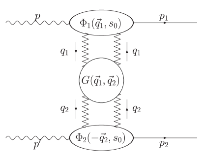
Figure 1: Schematic representation of the amplitude for the $\gamma^{*}(p)\,\gamma^{*}(p^{\prime})\to V(p_{1})\,V(p_{2})$ scattering.

2 Representations of the NLA amplitude

The process under consideration is the production of two light vector mesons ($V=\rho^{0},\omega,\phi$) in the collision of two virtual photons, $\gamma^{*}(p)\>\gamma^{*}(p^{\prime})\to V(p_{1})\>V(p_{2})$. Here, neglecting the meson mass $m_{V}$, $p_{1}$ and $p_{2}$ are taken as Sudakov vectors satisfying $p_{1}^{2}=p_{2}^{2}=0$ and $2(p_{1}p_{2})=s$; the virtual photon momenta are instead $p=\alpha p_{1}-Q_{1}^{2}/(\alpha s)p_{2}$ and $p^{\prime}=\alpha^{\prime}p_{2}-Q_{2}^{2}/(\alpha^{\prime}s)p_{1}$, so that the photon virtualities turn to be $p^{2}=-Q_{1}^{2}$ and $(p^{\prime})^{2}=-Q_{2}^{2}$. We consider the kinematics when $s\gg Q^{2}_{1,2}\gg\Lambda^{2}_{QCD}$ and $\alpha=1+Q_{2}^{2}/s+{\cal O}(s^{-2})$, $\alpha^{\prime}=1+Q_{1}^{2}/s+{\cal O}(s^{-2})$. In this case vector mesons are produced by longitudinally polarized photons in the longitudinally polarized state [6]. Other helicity amplitudes are power suppressed, with a suppression factor $\sim m_{V}/Q_{1,2}$. We will discuss here the amplitude of the forward scattering, i.e. when the transverse momenta of produced $V$ mesons are zero or when the variable $t=(p_{1}-p)^{2}$ takes its maximal value $t_{0}=-Q_{1}^{2}Q_{2}^{2}/s+{\cal O}(s^{-2})$.

In Ref. [9] the NLA forward amplitude has been written as a spectral decomposition on the basis of eigenfunctions of the LLA BFKL kernel:

$$\frac{\mbox{Im}_{s}\left({\cal A}\right)}{D_{1}D_{2}}=\frac{s}{(2\pi)^{2}}\int\limits^{+\infty}_{-\infty}d\nu\left(\frac{s}{s_{0}}\right)^{\bar{\alpha}_{s}(\mu_{R})\chi(\nu)}\alpha_{s}^{2}(\mu_{R})c_{1}(\nu)c_{2}(\nu)\left[1+\bar{\alpha}_{s}(\mu_{R})\left(\frac{c^{(1)}_{1}(\nu)}{c_{1}(\nu)}+\frac{c^{(1)}_{2}(\nu)}{c_{2}(\nu)}\right)\right.$$

$$\left.+\bar{\alpha}_{s}^{2}(\mu_{R})\ln\left(\frac{s}{s_{0}}\right)\left(\bar{\chi}(\nu)+\frac{\beta_{0}}{8N_{c}}\chi(\nu)\left[-\chi(\nu)+\frac{10}{3}+i\frac{d\ln(\frac{c_{1}(\nu)}{c_{2}(\nu)})}{d\nu}+2\ln(\mu_{R}^{2})\right]\right)\right]\;.$$ (1)

Here, ${\bar{\alpha}_{s}}=\alpha_{s}N_{c}/\pi$ and $D_{1,2}=-4\pi e_{q}f_{V}/(N_{c}Q_{1,2})$, where $f_{V}$ is the meson dimensional coupling constant ($f_{\rho}\approx 200\,\rm{MeV}$) and $e_{q}$ should be replaced by $e/\sqrt{2}$, $e/(3\sqrt{2})$ and $-e/3$ for the case of $\rho^{0}$, $\omega$ and $\phi$ meson production, respectively. We refer to Ref. [9] for the details of the derivation and for the definition of the functions of $\nu$ entering this expression. Two energy scales enter the expression (1), the renormalization scale $\mu_{R}$ and the scale $s_{0}$, which is an artificial scale introduced in the BFKL approach at the time to perform the Mellin transform from the $s$-space to the complex angular momentum plane.

It is easy to see that the above expression can be organized as a series:

$$\frac{Q_{1}Q_{2}}{D_{1}D_{2}}\frac{\mbox{Im}_{s}({\cal A}_{\mathrm{s}eries})}{s} = \frac{1}{(2\pi)^{2}}\alpha_{s}(\mu_{R})^{2}$$

$$\times \biggl{[}b_{0}+\sum_{n=1}^{\infty}\bar{\alpha}_{s}(\mu_{R})^{n}\,b_{n}\,\biggl{(}\ln\left(\frac{s}{s_{0}}\right)^{n}+d_{n}(s_{0},\mu_{R})\ln\left(\frac{s}{s_{0}}\right)^{n-1}\biggr{)}\biggr{]}\;.$$

The $b_{n}$ coefficients are determined by the kernel and the impact factors in LLA, while the $d_{n}$ coefficients depend also on the NLA corrections to the kernel and to the impact factors. For their expression, see Ref. [9].

An alternative possibility to represent the NLA amplitude is obtained by exponentiating the bulk of the kernel NLA corrections,

$$\frac{\mbox{Im}_{s}\left({\cal A}_{\mathrm{e}xp}\right)}{D_{1}D_{2}}=\frac{s}{(2\pi)^{2}}\int\limits^{+\infty}_{-\infty}d\nu\left(\frac{s}{s_{0}}\right)^{\bar{\alpha}_{s}(\mu_{R})\chi(\nu)+\bar{\alpha}_{s}^{2}(\mu_{R})\left(\bar{\chi}(\nu)+\frac{\beta_{0}}{8N_{c}}\chi(\nu)\left[-\chi(\nu)+\frac{10}{3}\right]\right)}\alpha_{s}^{2}(\mu_{R})c_{1}(\nu)c_{2}(\nu)$$

$$\times\!\left[1+\bar{\alpha}_{s}(\mu_{R})\left(\frac{c^{(1)}_{1}(\nu)}{c_{1}(\nu)}+\frac{c^{(1)}_{2}(\nu)}{c_{2}(\nu)}\right)+\bar{\alpha}_{s}^{2}(\mu_{R})\ln\left(\frac{s}{s_{0}}\right)\frac{\beta_{0}}{8N_{c}}\chi(\nu)\left(i\frac{d\ln(\frac{c_{1}(\nu)}{c_{2}(\nu)})}{d\nu}+2\ln(\mu_{R}^{2})\right)\right].$$ (3)

This form of the NLA amplitude was used in [20] (see also [21]), without account of the last two terms in the second line of (3), for the analysis of the total $\gamma^{*}\gamma^{*}$ cross section. We will refer in the following to this representation simply as “exponentiated” amplitude.

It is easily seen that the amplitude, in any of the given representations, is independent in the NLA from the choice of $s_{0}$ and of $\mu_{R}$ [9].

3 Numerical results

In Ref. [9] we presented some numerical results for the amplitude given in Eq. (2) for the $Q_{1}=Q_{2}\equiv Q$ kinematics, i.e. in the “pure” BFKL regime. We found that the $d_{n}$ coefficients are negative and increasingly large in absolute values as the perturbative order increases, making evident the need of an optimization of the perturbative series. We adopted the principle of minimal sensitivity (PMS) [10], by requiring the minimal sensitivity of the predictions to the change of both the renormalization and the energy scales, $\mu_{R}$ and $s_{0}$. We considered the amplitude for $Q^{2}$=24 GeV² and $n_{f}=5$ and studied its sensitivity to variation of the parameters $\mu_{R}$ and $Y_{0}=\ln(s_{0}/Q^{2})$. We could see that for each value of $Y=\ln(s/Q^{2})$ there are quite large regions in $\mu_{R}$ and $Y_{0}$ where the amplitude is practically independent on $\mu_{R}$ and $Y_{0}$ and we got for the amplitude a smooth behaviour in $Y$ (see the curve labeled “series - PMS” in Figs. 2 and 3). The optimal values turned out to be $\mu_{R}\simeq 10Q$ and $Y_{0}\simeq 2$, quite far from the kinematical values $\mu_{R}=Q$ and $Y_{0}=0$. These “unnatural” values probably mimic large unknown NNLA corrections.

Figure 2: $\mbox{Im}_{s}({\cal A})Q^{2}/(s\,D_{1}D_{2})$ as a function of $Y$ at $Q^{2}$=24 GeV² ($n_{f}=5$): (left) series representation with PMS and “exponentiated” representation with PMS, (right) series representation with PMS and with FAC.

As an estimation of the systematic effects in our determination, we want to consider here also the “exponentiated” representation of the amplitude, Eq. (3), and different optimization methods.

At first, we compare the series and the “exponentiated” determinations using in both case the PMS method. The optimal values of $\mu_{R}$ and $Y_{0}$ for the “exponentiated” amplitude are quite similar to those obtained in the case of the series representation, with only a slight decrease of the optimal $\mu_{R}$. Fig. 2 (left) shows that the two determinations are in good agreement at the lower energies, but deviate increasingly for large values of $Y$. It should be stressed, however, that the applicability domain of the BFKL approach is determined by the condition $\bar{\alpha}_{s}(\mu_{R})Y\sim 1$ and, for $Q^{2}$=24 GeV² and for the typical optimal values of $\mu_{R}$, one gets from this condition $Y\sim 5$. Around this value the discrepancy between the two determinations is within a few percent.

As a second check, we changed the optimization method and applied it both to the series and to the “exponentiated” representation. The method considered is the fast apparent convergence (FAC) method [11], whose strategy, when applied to a usual perturbative expansion, is to fix the renormalization scale to the value for which the highest order correction term is exactly zero. In our case, the application of the FAC method requires an adaptation, for two reasons: the first is that we have two energy parameters in the game, $\mu_{R}$ and $Y_{0}$, the second is that, if only strict NLA corrections are taken, the amplitude does not depend at all on these parameters. For details about the application of this method, we refer to [22]. Here, we merely show the results: the FAC method applied to the series representation (see Fig. 2 (right)) and to the exponentiated representation (see Fig. 3 (left)) gives results in nice agreement with those from the PMS method applied to the series representation, over the whole energy range considered.

Figure 3: $\mbox{Im}_{s}({\cal A})Q^{2}/(s\,D_{1}D_{2})$ as a function of $Y$ at $Q^{2}$=24 GeV² ($n_{f}=5$): (left) series representation with PMS and “exponentiated” representation with FAC, (right) series representation with PMS and with BLM.

Another popular optimization method is the Brodsky-Lepage-Mackenzie (BLM) one [12], which amounts to perform a finite renormalization to a physical scheme and then to choose the renormalization scale in order to remove the $\beta_{0}$-dependent part. We applied this method only to the series representation, Eq. (2). The result is compared with the PMS method in Fig. 3 (right) (for details, see Ref. [22]).

The $\gamma^{*}\gamma^{*}\to\rho\rho$ amplitude with the inclusion of NLA BFKL effects has been studied also in Ref. [19]. In that paper, the amplitude has been built with the following ingredients: leading-order impact factors for the $\gamma^{*}\to\rho$ transition, BLM scale fixing for the running of the coupling in the prefactor of the amplitude (the BLM scale is found using the NLA $\gamma^{*}\to\rho$ impact factor calculated in Ref. [6]) and renormalization-group-resummed BFKL kernel, with resummation performed on the LLA BFKL kernel at fixed coupling [23]. In Ref. [19] the behaviour of $d\sigma/dt$ at $t=t_{0}$ as a function of $\sqrt{s}$ was determined for three values of the common photon virtuality, $Q$=2, 3 and 4 GeV.

In order to make a comparison with the findings of Ref. [19], we computed $d\sigma/dt$ at $t=t_{0}$ for $Q$=2 and $Q$=4 GeV as functions of $\sqrt{s}$. We used $f_{\rho}$=216 MeV, $\alpha_{\mathrm{EM}}=1/137$ and the two–loop running strong coupling corresponding to the value $\alpha_{s}(M_{Z})=0.12$. The results are shown in the linear-log plots of Fig. 4, which shows a large disagreement. It would be interesting to understand to what extent this disagreement is due to the use in Ref. [19] of LLA impact factors instead of the NLA ones or to the way the collinear improvement of the kernel is performed.

The work of D.I. was partially supported by grants RFBR-05-02-1611, NSh-5362.2006.2.

Figure 4: $\left.d\sigma/dt\right|_{t=t_{0}}$ [pb/GeV²] as a function of $\sqrt{s}$ at $Q^{2}$=16 GeV² ($n_{f}=5$) (left) and at $Q^{2}$=4 GeV² ($n_{f}=3$) (right) from the series representation with the PMS optimization method (solid lines) compared with the determination from the approach in Ref. [19] (dashed lines).

References

- [1] V.S. Fadin, E.A. Kuraev, L.N. Lipatov, Phys. Lett. B60 (1975) 50; E.A. Kuraev, L.N. Lipatov and V.S. Fadin, Zh. Eksp. Teor. Fiz. 71 (1976) 840 [Sov. Phys. JETP 44 (1976) 443]; 72 (1977) 377 [45 (1977) 199]; Ya.Ya. Balitskii and L.N. Lipatov, Sov. J. Nucl. Phys. 28 (1978) 822.
- [2] V.S. Fadin and L.N. Lipatov, Phys. Lett. B429 (1998) 127; M. Ciafaloni and G. Camici, Phys. Lett. B430 (1998) 349.
- [3] V.S. Fadin and R. Fiore, Phys. Lett. B610 (2005) 61 [Erratum-ibid. B621 (2005) 61]; Phys. Rev. D72 (2005) 014018.
- [4] V.S. Fadin, R. Fiore, M.I. Kotsky and A. Papa, Phys. Rev. D61 (2000) 094005; Phys. Rev. D61 (2000) 094006; M. Ciafaloni and G. Rodrigo, JHEP 0005 (2000) 042.
- [5] J. Bartels, D. Colferai and G.P. Vacca, Eur. Phys. J. C24 (2002) 83; Eur. Phys. J. C29 (2003) 235.
- [6] D. Yu. Ivanov, M.I. Kotsky and A. Papa, Eur. Phys. J. C38 (2004) 195; Nucl. Phys. (Proc. Suppl.) 146 (2005) 117.
- [7] J. Bartels, S. Gieseke and C. F. Qiao, Phys. Rev. D63 (2001) 056014 [Erratum-ibid. D65 (2002) 079902]; J. Bartels, S. Gieseke and A. Kyrieleis, Phys. Rev. D65 (2002) 014006; J. Bartels, D. Colferai, S. Gieseke and A. Kyrieleis, Phys. Rev. D66 (2002) 094017; J. Bartels, Nucl. Phys. (Proc. Suppl.) (2003) 116; J. Bartels and A. Kyrieleis, Phys. Rev. D70 (2004) 114003; V.S. Fadin, D.Yu. Ivanov and M.I. Kotsky, Phys. Atom. Nucl. 65 (2002) 1513 [Yad. Fiz. 65 (2002) 1551]; V.S. Fadin, D.Yu. Ivanov and M.I. Kotsky, Nucl. Phys. B658 (2003) 156.
- [8] G. Chachamis, these proceedings.
- [9] D. Yu. Ivanov and A. Papa, Nucl. Phys. B 732 (2006) 183; hep-ph/0510397.
- [10] P.M. Stevenson, Phys. Lett. B100 (1981) 61; Phys. Rev. D23 (1981) 2916.
- [11] G. Grunberg, Phys. Lett. B95 (1980) 70 [Erratum-ibid. B110 (1982) 501]; ibid. B114 (1982) 271; Phys. Rev. D29 (1984) 2315.
- [12] S.J. Brodsky, G.P. Lepage, P.B. Mackenzie, Phys. Rev. D28 (1983) 228.
- [13] G.P. Salam, JHEP 9807 (1998) 019.
- [14] M. Ciafaloni, D. Colferai, Phys. Lett. B452 (1999) 372; M. Ciafaloni, D. Colferai, G.P. Salam, Phys. Rev. D60 (1999) 114036, JHEP 9910 (1999) 017, JHEP 0007 (2000) 054; M. Ciafaloni, D. Colferai, G.P. Salam, A.M. Stasto, Phys. Lett. B576 (2003) 143, Phys. Rev. D68 (2003) 114003.
- [15] G. Altarelli, R.D. Ball, S. Forte, Nucl. Phys. B575 (2000) 313, Nucl. Phys. B599 (2001) 383, Nucl. Phys. B621 (2002) 359, Nucl. Phys. B674 (2003) 459.
- [16] R.S. Thorne, Phys. Rev. D60 (1999) 054031, Phys. Lett. B474 (2000) 372, Phys. Rev. D64 (2001) 074005.
- [17] A. Sabio-Vera, Nucl. Phys. B722 (2005) 65.
- [18] R. Peschanski, C. Royon, L. Schoeffel, Nucl. Phys. B716 (2005) 401.
- [19] R. Enberg, B. Pire, L. Szymanowski and S. Wallon, Eur. Phys. J. C45 (2006) 759.
- [20] S.J. Brodsky, V.S. Fadin, V.T. Kim, L.N. Lipatov, G.B. Pivovarov, JETP Lett. 76 (2002) 249.
- [21] S.J. Brodsky, V.S. Fadin, V.T. Kim, L.N. Lipatov, G.B. Pivovarov, JETP Lett. 70 (1999) 155.
- [22] D. Yu. Ivanov and A. Papa, hep-ph/0610042.
- [23] A. Khoze, A.D. Martin, M.G. Ryskin, W.J. Stirling, Phys. Rev. D70 (2004) 074013; hep-ph/0406135.