Neutrino Physics - Models for Neutrino Masses and Lepton Mixing

Abstract:

In these lecture notes we present mechanisms for the generation of Majorana neutrino masses and lepton mixing. We consider simple extensions of the Standard Model. Apart from a section about radiative mass generation, we put special emphasis on the seesaw mechanism and $\mu$–$\tau$ interchange symmetry.

1 Introduction

Scope of the lecture notes:

These notes comprise two hours of lecture. The style is rather elementary and detailed. Therefore, only a few subjects have been presented and the choice of subjects is rather subjective, reflecting the preferences of the author. The notes are intended to offer access to some sections of model building for neutrino masses and lepton mixing from where the interested reader can go on with more advanced literature.

General introductions to neutrino physics, with emphasis on neutrino oscillations, are found in [1]. For recent developments in models for neutrino masses and mixing see [2]. Ref. [3] contains aspects of both, phenomenology and theory, and could be used as reading complementary to the present notes. In Refs. [1, 2, 3] one can find extended bibliographies, whereas here we confine ourselves to work closely related the presented subjects. For reviews of the results of neutrino oscillation experiments see [4].

Introductory remarks:

The results of the neutrino oscillation experiments have shown that at least two neutrinos are massive and lepton mixing exists in analogy to quark mixing. What does this important finding—one of the most spectacular discoveries in the recent history of particle physics—mean for model building? To obtain a reasonable perspective one should take into account the following remarks. It is no problem to accommodate neutrino masses and mixing, the problem is rather to explain its characteristic features. Note that in the quark sector the mass and mixing problem is still unsolved, after so many decennia and despite numerous attempts. It could very well be that the mass problem is decoupled from mixing problem, i.e., perhaps one can find models which explain mixing but not the masses. The mass problem could be more fundamental than the mixing problem in the following sense. Some mixing angles might find an explanation in mass ratios, see for instance the conjecture that the Cabibbo angle is approximately given by $\sin\theta_{c}\simeq\sqrt{m_{d}/m_{s}}$ where $m_{d}$ and $m_{s}$ are the masses of the down and strange quark, respectively [5]. Some of the mixing angles in the lepton sector might be, in a first approximation, independent of fermion masses, for instance the atmospheric mixing angle $\theta_{\mathrm{atm}}$ might be $45^{\circ}$ and thus maximal, and the small angle $\theta_{13}$ could zero. The meaning of these angles will be explained in Section 2.

As for accommodating neutrino masses and mixing, one could add to the multiplets of the Standard Model right-handed neutrino singlets $\nu_{R}$, just as one has right-handed quark singlets in the SM, and require conservation of the total lepton number $L$. Then one would have in the lepton sector a complete analogy to the quark sector, with massive Dirac neutrinos and lepton mixing.

Why are we not happy with this picture? Each of the three series of charged fermions (up quarks, down quarks and charged leptons) has a strong hierarchy in the masses. For instance, in the up quark sector we have $m_{t}/m_{u}\sim 4\times 10^{4}$. Moreover, the quark (CKM) mixing matrix is not extremely far from the unit matrix. This is in accord with the idea that both the quark mass hierarchy and the CKM matrix being close to unity are founded in hierarchical structures of the up and down quark mass matrices. On the other hand, in the lepton sector it is true there is a strong hierarchy in the charged lepton masses with $m_{\tau}/m_{e}\sim 3500$, however, when compared with the neutrino masses, experiments tell us that the largest neutrino mass is about six orders magnitude smaller than the electron mass. Thus the relation between charged lepton masses and neutrino masses is very different from the relation between down and up quark masses. Furthermore, it came as a surprise that the lepton mixing or PMNS matrix is very far from unity. Consequently, one would like to understand the following issues:

1. Why are neutrino masses much smaller than charged lepton masses?
   There are two generic “proposals” for a solution of this problem:

   • The seesaw mechanism,

   • radiative neutrino masses.

2. Can one reproduce the special features of neutrino masses and lepton mixing? The special features are

   • a solar mixing angle of $\theta_{\odot}\simeq 34^{\circ}\!\!\raisebox{1.99168pt}{$\begin{array}[]{c}\scriptstyle+3^{\circ}\\[-8.53581pt] \scriptstyle-2^{\circ}\end{array}$},$ which is large but non-maximal,

   • an atmospheric mixing angle of $\theta_{\mathrm{atm}}\simeq 45^{\circ}\pm 8^{\circ}$, which is large and perhaps maximal,

   • a small element $U_{e3}$ of the lepton mixing matrix, with $|U_{e3}|^{2}\equiv s_{13}^{2}\lesssim 0.02$,

   • a small ratio of neutrino mass-squared differences $\Delta m_{\odot}^{2}/\Delta m_{\mathrm{atm}}^{2}\sim 0.03$.

The approximate ranges for the mixing angles refer to 90% confidence level and are taken from [4].

The framework:

The framework of the lectures is defined by the following assumptions:

• We consider simple extensions of the lepton sector of the SM, i.e., the considered gauge group is $G=SU(2)_{L}\times U(1)_{Y}$.

• As for extensions of the fermion sector, we take into account the addition of right-handed neutrino singlets.

• We discuss all possible extensions of the scalar sector, compatible with $G$.

• We use flavour symmetries for enforcing certain features of the PMNS matrix.

• We assume Majorana nature of the neutrinos.

At this point we emphasize that an important question is whether the explanation of the features F1–4 is independent of the general fermion mass problem. Here we assume that this is the case. Otherwise, one would necessarily have to start with Grand Unified Theories, where quark masses and the CKM matrix is inseparably connected with the problem of lepton masses and the PMNS matrix. Another interesting question, to be solved by future experiments, is how close to $45^{\circ}$ is the atmospheric mixing angle and how close to zero is the small angle $\theta_{13}$. For the time being, sizeable deviations of these angles from these values are allowed. However, if it turns out that the atmospheric mixing angle is very close to maximal and $\theta_{13}$ very close to zero, this could hint at a non-abelian flavour symmetry.

The plan of the lecture notes is as follows. In Section 2 we discuss Majorana mass terms and the parameterization of lepton mixing. Section 3 introduces extensions of the SM by right-handed neutrino singlets, together with the seesaw mechanism, and extensions by additional scalar multiplets. In Section 4 we consider the so-called $\mu$–$\tau$-symmetry in the neutrino mass matrix. A model which realizes this symmetry is constructed in Section 5. Finally, in Section 6 we present some general considerations about about multi-Higgs models, with soft breaking of lepton numbers in the mass terms of the right-handed neutrino singlets.

2 Majorana neutrinos and lepton mixing

Majorana mass terms:

We begin with some algebra. All spinors used here are 4-spinors. In the space of 4-spinors the charge-conjugation matrix $C$ is defined by

$$C^{-1}\gamma_{\mu}C=-\gamma_{\mu}^{T},$$ (1)

where the $\gamma_{\mu}$ denote the Dirac matrices. We will always work in a representation of the Dirac matrices where $\gamma_{0}$ is hermitian and the $\gamma_{j}$ ($j=1,2,3$) are anti-hermitian. The properties of $C$ are

$$C^{T}=-C,\quad C^{\dagger}=C^{-1}.$$ (2)

Whereas the first property follows from Eq. (1) alone, the second one takes into account the hermiticity assumption.

The charge-conjugation operation is defined by

$$\psi^{c}\equiv C{\bar{\psi}}^{T}=C\gamma_{0}^{T}\psi^{*}.$$ (3)

The projectors

$$P_{L}\equiv(\mathbbm{1}-\gamma_{5})/2,\quad P_{R}\equiv(\mathbbm{1}+\gamma_{5})/2$$ (4)

produce so-called chiral 4-spinors. A spinor $\psi_{L}$ is called left-handed if $P_{L}\psi_{L}=\psi_{L}$. Then, using $C^{-1}\gamma_{5}C=\gamma_{5}^{T}$, it is easy to show that

$$P_{R}\left(\psi_{L}\right)^{c}=\left(\psi_{L}\right)^{c}.$$ (5)

Thus, a charge-conjugate chiral spinor has the opposite chirality.

A mass term is a Lorentz-invariant bilinear in the Lagangian. A Dirac mass term has the structure $\bar{\phi}_{R}\psi_{L}+\mbox{H.c.}$, with independent chiral spinors $\phi_{R}$, $\psi_{L}$. Note that in the mass term different chiralities are necessary, otherwise the mass term would be identically zero. If we have only one chiral spinor $\psi_{L}$ at our disposal, we can use Eq. (3) to form a right-handed spinor. In this way, we obtain a Majorana mass term (see also [3])

$$-\frac{1}{2}m\left(\overline{\left(\psi_{L}\right)^{c}}\psi_{L}+\mbox{H.c.}\right)=\frac{1}{2}m\psi_{L}^{T}C^{-1}\psi_{L}+\mbox{H.c.}$$ (6)

The spinors transform as

$$\psi_{L}\to\exp\left(-i\alpha_{\mu\nu}\sigma^{\mu\nu}/4\right)\psi_{L}\quad\mbox{with}\quad\sigma^{\mu\nu}=\frac{i}{2}\,\left[\gamma^{\mu},\gamma^{\nu}\right]$$ (7)

under Lorentz transformations, where the transformations are parameterized by the six coefficients of the real antisymmetric matrix $\left(\alpha_{\mu\nu}\right)$. Invariance of the term (6) is guaranteed because

$$\exp\left(-i\alpha_{\mu\nu}\sigma^{\mu\nu}/4\right)^{T}C^{-1}\exp\left(-i\alpha_{\lambda\rho}\sigma^{\lambda\rho}/4\right)=C^{-1}\quad\mbox{due to}\quad C\left(\sigma^{\mu\nu}\right)^{T}C^{-1}=-\sigma^{\mu\nu}.$$ (8)

The factor $1/2$ in Eq. (6) is necessary in order to interpret $m$ as the mass appearing in the Dirac equation because this factor is canceled in the functional derivative of the Lagrangian with respect to $\psi_{L}$ since it occurs twice (see second part of Eq. (6)).

Mass term for Majorana neutrinos:

According to the discussion above, we write down a Majorana neutrino mass term

$$\mathcal{L}_{\mathrm{maj}}=\frac{1}{2}\,\nu_{L}^{T}C^{-1}\mathcal{M}_{\nu}\nu_{L}+\mbox{H.c.},$$ (9)

where $\nu_{L}$ contains an arbitrary number of left-handed neutrino fields. Since fermion fields are anticommuting and $C$ is antisymmetric, we have $\nu_{aL}^{T}C^{-1}\nu_{bL}=\nu_{bL}^{T}C^{-1}\nu_{aL}$, where $\nu_{aL}$, $\nu_{bL}$ are 4-spinor neutrino fields occurring in $\nu_{L}$. Therefore, the neutrino mass matrix $\mathcal{M}_{\nu}$ is a symmetric matrix, i.e.

$$\mathcal{M}_{\nu}^{T}=\mathcal{M}_{\nu},$$ (10)

which is complex in general.

The diagonalization of this mass matrix proceeds according to a theorem, first proven by Schur [6]: For any symmetric and complex matrix $\mathcal{M}_{\nu}$ there exists a unitary matrix $V$ such that

$$V^{T}\mathcal{M}_{\nu}V=\hat{m}\equiv\mbox{diag}\,(m_{1},m_{2},m_{3}),$$ (11)

where the $m_{j}$, the neutrino masses, are real and non-negative. The matrix $V$ can be decomposed as

$$V=e^{i\hat{\varphi}}\,U\,\mbox{diag}\,(e^{i\rho},e^{i\sigma},1),$$ (12)

with a diagonal phase matrix $e^{i\hat{\varphi}}$. The neutrino mass eigenfields $\hat{\nu}_{L}$ are then given by the relation $\nu_{L}=V\hat{\nu}_{L}$, with Majorana fields and mass term given by

$$\nu_{M}=\hat{\nu}_{L}+\left(\hat{\nu}_{L}\right)^{c},\quad\mathcal{L}_{\mathrm{maj}}=\frac{1}{2}\,{\hat{\nu}}_{L}^{T}C^{-1}\hat{m}\hat{\nu}_{L}+\mbox{H.c.},$$ (13)

respectively. The Majorana fields $\nu_{M}$ fulfill $\left(\hat{\nu}_{M}\right)^{c}=\hat{\nu}_{M}$.

Let us from now on assume that we work in a basis where the charged lepton mass matrix is diagonal. Then the phases in $e^{i\hat{\varphi}}$ are unphysical in lepton mixing because they can be absorbed into the left-handed charged lepton fields in the following way. Consider the charged-current Lagrangian

$$-\mathcal{L}_{cc}=\frac{g}{\sqrt{2}}\,W^{-}_{\mu}\bar{\ell}_{L}\gamma^{\mu}\nu_{L}+\mbox{H.c.}=\frac{g}{\sqrt{2}}\,W^{-}_{\mu}\bar{\ell}_{L}\gamma^{\mu}V\hat{\nu}_{L}+\mbox{H.c.}$$ (14)

The charged-lepton fields $\ell=\ell_{L}+\ell_{R}$ are Dirac fields, thus their mass term is $\bar{\ell}_{R}\hat{m}_{\ell}\ell_{L}+\mbox{H.c.}$, where $\hat{m}_{\ell}$ is the diagonal mass matrix. Then, defining new fields $\ell^{\prime}_{L}=e^{-i\hat{\varphi}}\ell_{L}$ and $\ell^{\prime}_{R}=e^{-i\hat{\varphi}}\ell_{R}$, $e^{i\hat{\varphi}}$ disappears from $\mathcal{L}_{cc}$ without making reappearance in the mass term.

Note that the phase factors $e^{i\rho}$, $e^{i\sigma}$ of $V$ are physical for Majorana neutrinos and the phases $\rho$, $\sigma$ are called Majorana phases. We cannot absorb them in the neutrino fields, just as we absorbed $e^{i\hat{\varphi}}$ in the charged-lepton fields. If we absorb them in $\hat{\nu}_{1L}$, $\hat{\nu}_{2L}$, we shift the masses in Eq. (13) according to $m_{1}\to e^{-2i\rho}m_{1}$, $m_{2}\to e^{-2i\sigma}m_{2}$ and the new fields are not in the mass eigenbasis.

The lepton mixing matrix:

According to the discussion before, the lepton mixing matrix is given by

$$U_{\mathrm{PMNS}}=U\,\mbox{diag}\,(e^{i\rho},e^{i\sigma},1).$$ (15)

Using the convention of [7], we decompose the unitary matrix $U$ as

$$U=U_{23}U_{13}U_{12}=\left(\begin{array}[]{ccc}1&0&0\\ 0&c_{23}&s_{23}\\ 0&-s_{23}&c_{23}\end{array}\right)\left(\begin{array}[]{ccc}c_{13}&0&s_{13}e^{-i\delta}\\ 0&1&0\\ -s_{13}e^{i\delta}&0&c_{13}\end{array}\right)\left(\begin{array}[]{ccc}c_{12}&s_{12}&0\\ -s_{12}&c_{12}&0\\ 0&0&1\end{array}\right).$$ (16)

We use the abbreviations $c_{23}\equiv\cos\theta_{23}$, etc. The angle $\theta_{23}$ is also called atmospheric mixing angle because it is the protagonist in atmospheric and long-baseline $\nu_{\mu}\leftrightarrow\nu_{\tau}$ oscillations, with corresponding mass-squared difference $\Delta m^{2}_{\mathrm{atm}}$. The mixing angle $\theta_{13}$, for which only an upper bound exists, is responsible for $\nu_{e}\leftrightarrow\nu_{\mu}$ oscillations. The angle $\theta_{12}$ appears in solar or very long-baseline oscillations; the latter are at present only realized in the KamLAND experiment [4]. The corresponding mass-squared difference can always be chosen as $\Delta m^{2}_{\odot}=m_{2}^{2}-m_{1}^{2}$ with $m_{2}>m_{1}$. The phase $\delta$ is analogous to the CKM phase and can, in principle, be probed in neutrino oscillations [1].

With the convention $m_{2}>m_{1}$, there are two physically distinct cases for $m_{3}$: $m_{1}<m_{2}<m_{3}$, the “normal” spectrum, and $m_{3}<m_{1}<m_{2}$, the “inverted” spectrum. In both cases, $\Delta m^{2}_{\mathrm{atm}}$ can be chosen as the largest mass-squared difference.

3 Extensions of the SM

3.1 Right-handed neutrino singlets

Multiplets:

In this section we extend the set of SM fields by right-handed neutrino singlets. Thus we have $G$-multiplets with the following quantum numbers:

$$\begin{array}[]{cccll}&SU(2)&\!\!\times\!\!&\!U(1)&\\ D_{L}&\underline{\frac{1}{2}}&&Y=-1&\mbox{left-handed doublets,}\\ \ell_{R}&\underline{0}&&Y=-2&\mbox{right-handed charged lepton singlets,}\\ \nu_{R}&\underline{0}&&Y=\hphantom{-}0&\mbox{right-handed neutrino singlets,}\\ \phi&\underline{\frac{1}{2}}&&Y=\hphantom{-}1&\mbox{Higgs doublet,}\\ \tilde{\phi}&\underline{\frac{1}{2}}&&Y=-1&\mbox{Higgs doublet.}\end{array}$$

The irreducible representations of $SU(2)$ are denoted by weak isospin, $Y$ is the hypercharge. The scalar doublet $\tilde{\phi}$ is not an independent degree of freedom. It is related to $\phi$ by

$$\tilde{\phi}\equiv i\tau_{2}\phi^{*}\quad\mbox{or}\quad\phi=\left(\begin{array}[]{c}\phi^{+}\\ \phi^{0}\end{array}\right)\Leftrightarrow\tilde{\phi}=\left(\begin{array}[]{c}{\phi^{0}}^{*}\\ -\phi^{-}\end{array}\right),$$ (17)

where $\tau_{2}$ is the second Pauli matrix and in the second part of the equation we have assumed—without loss of generality—that the lower component in $\phi$ is the one with zero electric charge. Clearly, the hypercharge of $\tilde{\phi}$ is opposite to the hypercharge of $\phi$, but under $SU(2)$ both fields transform in the same way: suppose $U\in SU(2)$ and $\phi\to U\phi$, then also $\tilde{\phi}\to U\tilde{\phi}$. The reason is that

$$U^{\dagger}i\tau_{2}U^{*}=i\tau_{2}\Leftrightarrow U^{T}i\tau_{2}U=i\tau_{2},$$ (18)

which is a special $SU(2)$ property.

There are two motivations for introducing the $\nu_{R}$. First of all, in the SM the left-handed quark doublet fields have right-handed $SU(2)$-singlet partners. From that point of view there is no reason for omitting the $\nu_{R}$. Before the discovery of neutrino masses, the omission of $\nu_{R}$ was fine because in that way the neutrinos stayed massless. The second motivation comes from GUTs based on the gauge group $SO(10)$. In such models all chiral fermions of one family are contained in the 16-dimensional irreducible spinor representation. Let us do the counting of the chiral fields per family:

$2\times 2\times 3$ (quarks: up, down; L, R; colour) + $2\times 2$ (leptons: $\ell$, $\nu$; L, R) = 16

Thus, in $SO(10)$ GUTs the $\nu_{R}$ is automatically included. For an introduction into $SO(10)$ GUTs see for instance [8].

The Lagrangian:

Let us assume that we have the multiplets of the SM plus one $\nu_{R}$ per family; in addition, we allow for violations of all lepton numbers, including the total lepton number $L$, and an arbitrary number of Higgs doublets. Then the Lagrangian is given by

$$\mathcal{L}=\cdots-\sum_{j}\left[\bar{\ell}_{R}\phi_{j}^{\dagger}\Gamma_{j}+\bar{\nu}_{R}{\tilde{\phi}}^{\dagger}\Delta_{j}\right]D_{L}+\mbox{H.c.}+\left(\frac{1}{2}\,\nu_{R}^{T}C^{-1}\!M_{R}^{*}\nu_{R}+\mbox{H.c.}\right),$$ (19)

where the dots indicate the gauge part. The $\nu_{R}$ mass term is of Majorana form and is present because we allow for $L$-violation. The requirement of $L$ conservation would forbid that term and lead to Dirac neutrinos. In analogy to Eq. (10), we have $M_{R}=M_{R}^{T}$. Spontaneous symmetry breaking of the SM gauge group induces the mass matrices

$$M_{\ell}=\sum_{j}v_{j}^{\ast}\Gamma_{j}\,,\quad M_{D}=\sum_{j}v_{j}\Delta_{j}\quad\mbox{with}\quad\langle\phi_{j}^{0}\rangle_{0}=v_{j},$$ (20)

where $M_{\ell}$ is the mass matrix of the charged leptons and the $v_{j}$ are the vacuum expectation values (VEVs) of the Higgs doublets. The matrix $M_{D}$ goes together with $M_{R}$ to form a Majorana mass term for left-handed neutrino fields [9]:

$$\mathcal{L}_{\nu\,\mathrm{mass}}=\frac{1}{2}\,\omega_{L}^{T}C^{-1}\mathcal{M}_{D+M}\,\omega_{L}+\mbox{H.c.},$$ (21)

with the $6\times 6$ matrix

$$\mathcal{M}_{D+M}=\left(\begin{array}[]{cc}0&M_{D}^{T}\\ M_{D}&M_{R}\end{array}\right)\quad\mbox{and}\quad\omega_{L}=\left(\begin{array}[]{c}\nu_{L}\\ C(\bar{\nu}_{R})^{T}\end{array}\right).$$ (22)

Let us sketch the derivation of Eqs. (21) and (22). We have to reformulate all mass terms with $(\nu_{R})^{c}$. For this purpose we reformulate Eq. (3) as

$$\nu_{R}^{*}=-C^{-1}\gamma_{0}(\nu_{R})^{c},$$ (23)

from $(\nu_{R})^{cc}=\nu_{R}$ we derive

$$\bar{\nu}_{R}=\overline{(\nu_{R})^{cc}}=-[(\nu_{R})^{c}]^{T}C^{-1}$$ (24)

and from Eq. (1) we obtain

$$\gamma_{0}^{T}C^{-1}\gamma_{0}=-C^{-1}.$$ (25)

Using Eq. (24) we treat first the Dirac term:

$$-\bar{\nu}_{R}M_{D}\nu_{L}=[(\nu_{R})^{c}]^{T}C^{-1}M_{D}\nu_{L}=\frac{1}{2}\left\{[(\nu_{R})^{c}]^{T}C^{-1}M_{D}\nu_{L}+\nu_{L}^{T}C^{-1}M_{D}^{T}[(\nu_{R})^{c}]\right\}.$$ (26)

Dealing with the Majorana term, we first take its complex conjugate, then use Eq. (23) and finally Eq. (25):

$$\left(\frac{1}{2}\,\nu_{R}^{T}C^{-1}\!M_{R}^{*}\nu_{R}\right)^{\dagger}=\frac{1}{2}\,\nu_{R}^{\dagger}CM_{R}\nu_{R}^{*}=\frac{1}{2}\,[-C^{-1}\gamma^{0}(\nu_{R})^{c}]^{T}CM_{R}[-C^{-1}\gamma^{0}(\nu_{R})^{c}]=$$

$$\frac{1}{2}\,[(\nu_{R})^{c}]^{T}\left(-{\gamma^{0}}^{T}C^{-1}\gamma^{0}\right)M_{R}(\nu_{R})^{c}=\frac{1}{2}\,[(\nu_{R})^{c}]^{T}C^{-1}M_{R}(\nu_{R})^{c}.$$ (27)

Equations (26) and (27) are in exactly the form we to have.

The seesaw mechanism:

In the mass matrix (22), $M_{D}$ is generated by the VEVs of the Higgs doublets, therefore, its elements are at most of the order of the electroweak scale. On the other hand, the scale of $M_{R}$ is not protected by the gauge symmetry and there is no reason why it cannot be much larger. Indeed the basic assumption of the seesaw mechanism [10] is $m_{D}\ll m_{R}$, where $m_{D}$ and $m_{R}$ are the scales of $M_{D}$ and $M_{R}$, respectively. A more precise formulation of this assumption is that the largest eigenvalue of $\sqrt{M_{D}^{\dagger}M_{D}}$ is much smaller than the smallest eigenvalue of $\sqrt{M_{R}^{\dagger}M_{R}}$.

To derive the seesaw mechanism, we are looking for a unitary $6\times 6$ matrix $W$ which disentangles small from large scale. In the derivation we follow Ref. [11] and make the ansatz

$$W=\left(\begin{array}[]{cc}\sqrt{\mathbbm{1}-BB^{\dagger}}&B\\ -B^{\dagger}&\sqrt{\mathbbm{1}-B^{\dagger}B}\end{array}\right),$$ (28)

such that

$$W^{T}\mathcal{M}_{D+M}W=\left(\begin{array}[]{cc}\mathcal{M}_{\nu}&0\\ 0&\mathcal{M}_{\nu}^{\mathrm{heavy}}\end{array}\right)$$ (29)

The right-hand side of this equation expresses the disentanglement of small and large scales. The matrix $W$ is modeled after a $2\times 2$ rotation matrix. The square root is understood as Taylor expansion $\sqrt{1-x}=1-\frac{1}{2}\,x-\frac{1}{8}\,x^{2}-\cdots$. Before we go on we do some parameter counting. The matrix $B$ is a general complex $3\times 3$ matrix and thus has 18 real parameters, and $W$ has the same number of parameters. A general unitary $6\times 6$ matrix has 36 parameters. Thus $W$ has 18 parameters less and it is impossible to diagonalize $\mathcal{M}_{D+M}$ with $W$. The lack of 18 parameters agrees with the form of the matrix on the right-hand side of Eq. (29): $\mathcal{M}_{\nu}$ and $\mathcal{M}_{\nu}^{\mathrm{heavy}}$ are both symmetric and would need each a unitary $3\times 3$ matrix for diagonalization, thus $2\times 9=18$ further parameters.

Equation (29) determines $B$ as a function of $M_{D}$ and $M_{R}$, by requiring disentanglement:

$$\sqrt{\mathbbm{1}-B^{T}B^{*}}\,M_{D}\sqrt{\mathbbm{1}-B\,B^{\dagger}}-B^{T}M_{D}^{T}B^{\dagger}-\sqrt{\mathbbm{1}-B^{T}B^{*}}M_{R}B^{\dagger}=0.$$ (30)

By expanding $B$ in $m_{D}/m_{R}$, Eq. (30) allows for a recursive solution. One can show [11] that $B=B_{1}+B_{3}+B_{5}+\cdots$, where $B_{n}$ is of order $(m_{D}/m_{R})^{n}$. The first term in $B$ is easily obtained from Eq. (30) as

$$B_{1}=\left(M_{R}^{-1}M_{D}\right)^{\dagger},$$ (31)

and up to second order [12]

$$W\simeq\left(\begin{array}[]{cc}1-\frac{1}{2}\,B_{1}B_{1}^{\dagger}&B_{1}\\ -B_{1}^{\dagger}&1-\frac{1}{2}\,B_{1}^{\dagger}B_{1}\end{array}\right).$$ (32)

Then one finds the leading term of the light-neutrino mass matrix [10]:

$$\mathcal{M}_{\nu}=-M_{D}^{T}M_{R}^{-1}M_{D}.$$ (33)

This is the famous seesaw formula. In leading order, the mass matrix of heavy neutrinos is given by

$$\mathcal{M}_{\nu}^{\mathrm{heavy}}=M_{R}.$$ (34)

An interesting feature is that corrections to $\mathcal{M}_{\nu}$ and $\mathcal{M}_{\nu}^{\mathrm{heavy}}$ suppressed by $(m_{D}/m_{R})^{2}$, i.e., by the square of the small ratio $m_{D}/m_{R}$ [11]. This is a consequence of the zero in the upper left corner of $\mathcal{M}_{D+M}$—see Eq. (22).

We note that the whole procedure sketched here goes through with an arbitrary number of right-handed neutrinos. We could choose for instance two or more than three $\nu_{R}$. However, if we chose only one right-handed neutrino, then two neutrino masses are zero, which is in disagreement with the two non-zero mass-squared differences; in this case an additional contribution to the neutrino masses has to be supplied from elsewhere.

Let us for the moment assume that the charged-lepton mass matrix is non-diagonal and it gets diagonalized by $(U_{R}^{\ell})^{\dagger}M_{\ell}U_{L}^{\ell}=\hat{m}_{\ell}$. In that case the lepton mixing matrix is given by $U_{M}=(U_{L}^{\ell})^{\dagger}V$ and there are three sources for mixing: $M_{\ell}$, $M_{D}$ and $M_{R}$. Thus the seesaw mechanism is a rich playground for model building.

To conclude the seesaw part, we want make a scale consideration. Choose as a typical neutrino mass $m_{\nu}\sim\sqrt{\Delta m^{2}_{\mathrm{atm}}}\sim 0.05$ eV and $m_{D}\sim m_{\mu,\tau}$. Then, $m_{R}\sim 10^{8}\div 10^{11}$ GeV. This is fairly close to the GUT scale. Could the seesaw scale $m_{R}$ be identical with a GUT scale of typically $M_{\mathrm{GUT}}\simeq 2\times 10^{16}$ GeV? This is not possible without some amount of finetuning because $m_{D}\lesssim v$, where the VEV $v\simeq 174$ GeV represents the electroweak scale. Then, according to the seesaw mechanism $m_{\nu}\sim v^{2}/M_{\mathrm{GUT}}\sim 1.5\times 10^{-3}$ eV, which is too small. On the other hand, in the minimal SUSY extension of the SM gauge coupling unification happens at $M_{\mathrm{GUT}}$ and the question is if in a certain GUT model an intermediate scale like the seesaw scale is allowed. It has been shown that the so-called minimal SUSY $SO(10)$ GUT is ruled out for this reason [13]. This problem is an interesting research topic.

3.2 Additional scalar multiplets

The leptonic SM multiplets are characterized in the beginning of Section 3.1. With these multiplets one can form leptonic bilinears with the following quantum numbers [14]:

$$\begin{array}[]{cr@{\,=\,}lccl}\bar{D}_{L}\otimes\ell_{R}&\underline{\frac{1}{2}}\otimes\underline{0}&\underline{\frac{1}{2}}&Y=-1&\>\phi&\mbox{doublet}\,\,Y=+1,\\ D_{L}\otimes D_{L}&\underline{\frac{1}{2}}\otimes\underline{\frac{1}{2}}&\underline{0}\oplus\underline{1}&Y=-2&\left\{\begin{array}[]{c}\eta^{+}\\ \!\!\Delta\end{array}\right.&\!\!\!\begin{array}[]{l}\mbox{singlet}\,\,\,\,Y=+2,\\ \mbox{triplet}\,\,\,\,Y=+2,\end{array}\\ \ell_{R}\otimes\ell_{R}&\underline{0}\otimes\underline{0}&\underline{0}&Y=-4&\quad k^{++}&\mbox{singlet}\,\,\,Y=+4.\end{array}$$

This is the complete SM list. One can add $\nu_{R}\otimes\nu_{R}$ with trivial quantum numbers $\underline{0}\otimes\underline{0}=\underline{0},\>Y=0$, which tells us that this bilinear can couple to a real or complex scalar singlet. We will not consider this possibility in these lecture notes.

In the list above, apart from the trivial case with weak isospin $1/2$, there are three interesting new scalar multiplets, which enable massive Majorana neutrinos. Three such models, corresponding to these multiplets, will be discussed in the following.

The Zee model:

The essential ingredient of this model is the charged scalar $\eta^{+}$ [15, 16]. In addition to the SM multiplets, it needs a second Higgs doublet. The relevant parts of the Lagrangian are

$$\mathcal{L}=\cdots+f_{\alpha\beta}D_{\alpha L}^{T}C^{-1}i\tau_{2}D_{\beta L}\,\eta^{+}-\mu\,\phi_{1}^{\dagger}\tilde{\phi}_{2}\eta^{+}+\mbox{H.c.},$$ (35)

where $f_{\alpha\beta}$ is the Yukawa coupling matrix of $\eta^{+}$. Without loss of generality we can assume that the charged-lepton mass matrix is diagonal and, therefore, $\alpha$ and $\beta$ indicate the flavour, i.e., $\alpha,\,\beta=e,\,\mu,\,\tau$. The $\eta^{+}$ Yukawa interaction has a “Majorana” structure and is Lorentz-invariant just as the Majorana mass term discussed in Section 2. The Pauli matrix $\tau_{2}$ acts on the $SU(2)$ doublets $D_{\beta L}$, i.e., it has $SU(2)$ indices. Equation (18) expresses the invariance of the $\eta^{+}$ Yukawa interaction under $SU(2)$.

In Section 2 we have derived that a Majorana mass matrix is symmetric—see Eq. (10). We can apply an analogous reasoning here, however, due to the antisymmetry of $\tau_{2}$, we have

$$D_{\alpha L}^{T}C^{-1}i\tau_{2}D_{\beta L}=-D_{\beta L}^{T}C^{-1}i\tau_{2}D_{\alpha L}\quad\mbox{and}\quad f_{\alpha\beta}=-f_{\beta\alpha}.$$ (36)

Why does the Zee model need two Higgs doublets? The Zee model aims at radiative neutrino mass generation. Since there is no $\nu_{R}$, the neutrinos have to be of the Majorana type, with violation of the total lepton number $L$. Therefore, a necessary condition for non-zero neutrino masses in the Zee model is $L$-violation. Considering the $\eta^{+}$ Yukawa interaction in Eq. (35) and the Yukwawa interactions of the Higgs doublets, leads us to the following lepton number assignment:

$$\begin{array}[]{c|cccc}&D_{L}&\ell_{R}&\phi_{1,2}&\eta^{+}\\ \hline\cr L&1&1&0&-2\end{array}$$

Clearly, such a lepton number is explicitly broken by the $\mu$-term in Eq. (35), and this is the only term in the total Lagrangian which breaks $L$. Suppose we have only one Higgs doublet, i.e., $\phi_{1}=\phi_{2}\equiv\phi$. Then it follows that $\phi_{1}^{\dagger}\tilde{\phi}_{2}=\phi^{\dagger}\tilde{\phi}\equiv 0$ and the $\mu$-term is absent and without it the neutrinos remain massless.

A restricted version of Zee model has been proposed by Wolfenstein [17]. In that version only $\phi_{1}$ couples to leptons. This is guaranteed if we introduce the symmetry

$$D_{L}\to iD_{L},\quad\ell_{R}\to i\ell_{R},\quad\phi_{1}\to\phi_{1},\quad\phi_{2}\to-\phi_{2},\quad\eta^{+}\to-\eta^{+}.$$ (37)

Note that in this case the Yukawa coupling matrix of $\phi_{1}$ is proportional to the diagonal mass matrix of the charged leptons. The 1-loop Feynman diagram which generates neutrino masses is depicted in Fig. 1.

Figure 1: The 1-loop Feynman diagram for the generation of neutrino masses in the Zee model.

The vertex at the right corner of the diagram has a charged-lepton mass from the Yukawa coupling, another one comes from the mass insertion on the fermion line. The diagram describes a transition $\nu_{L}\to\left(\nu_{L}\right)^{c}$, in accord with a Majorana mass term—see Eq. (6). Taking into account that $\mathcal{M}_{\nu}$ is symmetric, one finds [15]

$$\mathcal{M}_{\nu}\propto\left((m_{\alpha}^{2}-m_{\beta}^{2})f_{\alpha\beta}\right)\quad\mbox{or}\quad\mathcal{M}_{\nu}=\left(\begin{array}[]{ccc}0&a&b\\ a&0&c\\ b&c&0\end{array}\right).$$ (38)

Thus the restricted version of the Zee model generates the most general Majorana mass matrix with zeros on the diagonal. After removal of unphysical phases, one obtains a real 3-parameter mass matrix. However, the mass matrix (38) is not viable [18], because it predicts that solar mixing is, for all practical purposes, maximal.

Thus the restricted version is ruled out. However, if both Higgs doublets are allowed to couple in the lepton sector, i.e., there are two different coupling matrices at the right corner of the diagram in Fig. 1, then $\mathcal{M}_{\nu}$ has in general non-zero entries in the diagonal, non-maximal solar mixing is allowed and there is no contradiction with experimental results [19]. On the other hand, though neutrino masses are suppressed because they are generated radiatively, further suppression is required to get neutrino masses of order 1 eV. If we perform such a suppression by small Yukawa couplings of the $\eta^{+}$, a rough estimate is $|f_{\alpha\beta}|\lesssim 10^{-4}$.

The Zee–Babu model:

In this model [16, 20], the SM multiplets are enriched by the scalar singlets $\eta^{+}$ and $k^{++}$. The relevant parts of the Lagrangian are given by

$$\mathcal{L}=\cdots+f_{\alpha\beta}D_{\alpha L}^{T}C^{-1}i\tau_{2}D_{\beta L}\,\eta^{+}+h_{\alpha\beta}\ell_{\alpha R}^{T}C^{-1}\ell_{\beta R}\,k^{++}-\tilde{\mu}\,\eta^{-}\eta^{-}k^{++}+\mbox{H.c.}$$ (39)

Now we use arguments similar to those for the Zee model. The Yukawa coupling matrix of $k^{++}$ has the property

$$h_{\alpha\beta}=h_{\beta\alpha}.$$ (40)

If we assign lepton numbers $L$, then $L(k^{++})=-2$, but $L$ is explicitly broken by the $\tilde{\mu}$-term. Thus, we obtain radiative neutrino masses, with neutrinos of the Majorana type.

The Zee–Babu model has only one Higgs doublet. According to the discussion of the Zee model, at 1-loop the neutrino masses are still zero, but they appear at the 2-loop level. The relevant Feynman diagram is depicted in Fig. 2. Examination of that diagram shows that

$$\mathcal{M}_{\nu}\propto\tilde{f}\hat{m}_{\ell}{\tilde{h}}^{*}\hat{m}_{\ell}\tilde{f},$$ (41)

with $\tilde{f}=(f_{\alpha\beta})$, $\tilde{h}=(h_{\alpha\beta})$ and $\hat{m}_{\ell}=\mbox{diag}\,(m_{e},m_{\mu},m_{\tau})$.

Figure 2: The 2-loop Feynman diagram for the generation of neutrino masses in the Zee–Babu model.

The properties of the model are the following. Since $\tilde{f}$ is antisymmetric, the lightest neutrino mass is zero. Assuming neutrino mass hierarchy requires the fine-tuning [21] $|h_{\mu\mu}|:|h_{\mu\tau}|:|h_{\tau\tau}|\simeq 1:(m_{\mu}/m_{\tau}):(m_{\mu}/m_{\tau})^{2}$. With scalar masses in the TeV range, small neutrino masses require $|f_{\alpha\beta}|$, $|h_{\alpha\beta}|\lesssim 0.1$. Thus, with 2-loop suppression, neutrino masses turn out to be naturally small. As a bonus, rare decays like $\tau\to 3\mu$ and $\mu\to e\gamma$ are within reach of forthcoming experiments.

We want to finish our discussion of the two models for radiative neutrino mass generation with a remark. Via the loop diagrams the hierarchy of the charged-lepton masses is transferred into the neutrino mass matrix, which is, therefore, naturally of hierarchical structure. Thus, finetuning of Yukawa couplings seems to be unavoidable in order to reproduce large lepton mixing.

The triplet model:

That model is obtained by enlarging the SM by a scalar triplet $\Delta$. This triplet is conveniently written as a $2\times 2$ matrix with $SU(2)$ indices, parameterized by

$$\Delta=\sum_{j=1}^{3}\delta_{j}\tau_{j},$$ (42)

where the $\tau_{j}$ are the Pauli matrices. The relevant terms of the Lagrangian are given by [22]

$$\mathcal{L}=\cdots+\frac{1}{2}g_{\alpha\beta}D_{L\alpha}^{T}C^{-1}i\tau_{2}\Delta D_{L\beta}+\mbox{H.c.}-M^{2}\mbox{Tr}\,\Delta^{\dagger}\Delta-\left(\mu_{\Delta}\,\phi^{\dagger}\Delta\tilde{\phi}+\mbox{H.c.}\right)-\cdots$$ (43)

The first dots indicate the gauge part, the second ones the missing terms of the scalar potential which are not relevant for our discussion. Observing that the $\tau_{2}\tau_{j}$ are symmetric for $j=1,2,3$, we find

$$g_{\alpha\beta}=g_{\beta\alpha}.$$ (44)

The triplet coupling is $SU(2)$-invariant for the following reason. With $U\in SU(2)$, the transformation properties are

$$D_{L}\to UD_{L},\quad\Delta\to U\Delta U^{\dagger}.$$ (45)

Using the parameterization (42), the latter equation demonstrates that $\vec{\delta}$ transforms according to the adjoint representation of $SU(2)$, i.e., as an $SU(2)$ triplet. Invariance under $SU(2)$ of the triplet term is again proved by using Eq. (18).

Let us now determine the charge-eigenfields of the triplet. First we note that its hypercharge is $Y_{\Delta}=2$. In general, the electric charge in a multiplet of the SM gauge group is given by $\mathbbm{Q}=T_{3}+\frac{1}{2}\,Y$, where $T_{3}$ is the third $SU(2)$ generator, i.e., the third component of weak isospin. According to Eq. (45), we thus obtain

$$\mathbbm{Q}\Delta=\frac{1}{2}\,[\tau_{3},\Delta]+\Delta$$ (46)

or

$$\left(\begin{array}[]{cc}\delta_{3}&\delta_{1}-i\delta_{2}\\ \delta_{1}+i\delta_{2}&-\delta_{3}\end{array}\right)\stackrel{{\scriptstyle\mathbbm{Q}}}{{\to}}\left(\begin{array}[]{cc}\delta_{3}&2\left(\delta_{1}-i\delta_{2}\right)\\ 0\left(\delta_{1}+i\delta_{2}\right)&-\delta_{3}\end{array}\right).$$ (47)

Therefore,

$$\Delta=\left(\begin{array}[]{cc}H^{+}&\sqrt{2}H^{++}\\ \sqrt{2}H^{0}&-H^{+}\end{array}\right),$$ (48)

with $H^{0}=\frac{1}{\sqrt{2}}\left(\delta_{1}+i\delta_{2}\right)$, $H^{+}=\delta_{3}$, $H^{++}=\frac{1}{\sqrt{2}}\left(\delta_{1}-i\delta_{2}\right)$.

Assigning lepton numbers as in the previous models, we find $L(\Delta)=-2$, and $L$ is explicitly broken by the $\mu_{\Delta}$-term. However, according to Eq. (48), the triplet has a neutral component which can have a VEV

$$\langle H^{0}\rangle_{0}=\frac{1}{\sqrt{2}}v_{T}.$$ (49)

Thus in the triplet model there is a tree-level neutrino mass matrix [22]

$$\mathcal{M}_{\nu}=v_{T}(g_{\alpha\beta}).$$ (50)

Since the triplet VEV disturbs the famous tree level relation $M_{W}/M_{Z}=\cos\theta_{W}$ for $W$ mass, $Z$ mass and Weinberg angle $\theta_{W}$, there is an upper bound $|v_{T}|/v\lesssim 0.03$ from the LEP data [23]. However, in order to have small enough neutrino masses from a small VEV, $v_{T}$ must be much smaller, namely $v_{T}\sim 0.1\div 1$ eV.

How to get a small $v_{T}$? Mechanisms in analogy to the seesaw mechanism, where the order of the neutrino masses is given by $m_{D}^{2}/m_{R}$ with $m_{D}\ll m_{R}$, have been proposed such that the triplet VEV is obtained by an analogous order of magnitude relation. Such mechanisms are usually called type II seesaw [24] (see also [8]). In that context the original seesaw mechanism is called type I. Here we follow Ref. [25]. We assume

$$M,\>|\mu_{\Delta}|\gg v,$$ (51)

where $v\simeq 174$ GeV is the VEV of the Higgs doublet. Replacing in the scalar potential of Eq. (43) the fields by the VEVs, we obtain

$$\langle V\rangle_{0}=M^{2}v_{T}^{*}v_{T}+v^{2}\mu_{\Delta}v_{T}+v^{2}\mu^{*}v_{T}^{*}+\cdots$$ (52)

The dots contain terms of order $v^{4}$ and $v_{T}^{2}v^{2}$. The stability condition with respect to $v_{T}$ requires

$$\frac{\partial}{\partial v_{T}^{*}}\langle V\rangle_{0}=M^{2}v_{T}+v^{2}\mu^{*}+\mathcal{O}(v_{T}v^{2})=0,$$ (53)

which results in

$$|v_{T}|\simeq|\mu|v^{2}/M^{2}.$$ (54)

Indeed, $v_{T}$ is of the form $v^{2}/m_{S}$, where $m_{S}$ is a large scale in the scalar sector. We want to emphasize that the mechanism for generating a small non-zero $v_{T}$ has a peculiar feature. It requires $M^{2}>0$, thus without the VEV of the Higgs doublet the triplet VEV would be zero. On the other hand, the VEV of $\phi$ is non-zero because in the scalar potential the term $\phi^{\dagger}\phi$ has a negative coefficient.

In summary, in the triplet model, generation of small neutrino masses requires a small triplet VEV $v_{T}$, which in turn requires a new new heavy scale in scalar sector, in analogy to the seesaw mechanism of type I. Seesaw mechanisms of type I+II are naturally obtained in $SO(10)$ GUTs, see for instance [8]. If both types are together, the mass matrix (22) looks like

$$\mathcal{M}_{D+M}=\left(\begin{array}[]{cc}M_{L}&M_{D}^{T}\\ M_{D}&M_{R}\end{array}\right),$$ (55)

with the seesaw formula

$$\mathcal{M}_{\nu}=M_{L}-M_{D}^{T}M_{R}^{-1}M_{D}.$$ (56)

Note that now all terms in $B=B_{1}+B_{2}+B_{3}+\cdots$ in an expansion in $1/m_{R}$ appear—see for instance [11], for a thorough discussion. The matrix $M_{L}$ need not necessarily be present at tree level, as it the case in the triplet model, but can also appear via loop corrections in some models—see for instance [26].

4 The $\mu$–$\tau$-symmetric neutrino mass matrix

We depart from the Majorana mass term (9) and the basis where charged-lepton mass matrix is diagonal. We consider the mass matrix

$$\mathcal{M}_{\nu}=\left(\begin{array}[]{ccc}x&y&y\\ y&z&w\\ y&w&z\end{array}\right)\quad\mbox{with}\quad x,\,y,\,z,\,w\in\mathbbm{C},$$ (57)

which is symmetric under $\mu$–$\tau$ interchange—for early references on this mass matrix see [27, 28].

The $\mu$–$\tau$ interchange symmetry in $\mathcal{M}_{\nu}$ can be defined as [29]

$$S\mathcal{M}_{\nu}S=\mathcal{M}_{\nu}\quad\mbox{with}\quad S=\left(\begin{array}[]{ccc}1&0&0\\ 0&0&1\\ 0&1&0\end{array}\right).$$ (58)

Let us now discuss the phenomenology of the mass matrix (57). We immediately guess one eigenvector:

$$\left(\begin{array}[]{ccc}x&y&y\\ y&z&w\\ y&w&z\end{array}\right)\left(\begin{array}[]{r}0\\ 1\\ -1\end{array}\right)=(z-w)\left(\begin{array}[]{r}0\\ 1\\ -1\end{array}\right).$$ (59)

Since this vector is real, it can be identified with one of the columns in the diagonalization matrix $V$, defined in Eq. (11). The first component of this eigenvector is zero, thus we identify it with the third column of $V$ because $|V_{e3}|=s_{13}$ (see Eqs. (12) and (16)) is compatible with zero. Therefore, we also obtain $m_{3}=|z-w|$. Inspecting $U$ of Eq. (16) we find with the eigenvector above that

$$\theta_{23}=45^{\circ},\quad\theta_{13}=0^{\circ},$$ (60)

and the parameter measured in atmospheric and long-baseline experiments is maximal, i.e.,

$$\sin^{2}2\theta_{\mathrm{atm}}=4\,|U_{\mu 3}|^{2}\left(1-|U_{\mu 3}|^{2}\right)=1.$$ (61)

Because of Eq. (60), the matrix $V$ is given by

$$V=\mathrm{diag}\,(e^{i\varphi_{e}},e^{i\varphi_{\mu}},-e^{i\varphi_{\mu}})\left(\begin{array}[]{ccc}\scriptstyle\cos\theta&\scriptstyle\sin\theta&\scriptstyle 0\\ -\frac{\sin\theta}{\sqrt{2}}&\frac{\cos\theta}{\sqrt{2}}&\frac{1}{\sqrt{2}}\\ -\frac{\sin\theta}{\sqrt{2}}&\frac{\cos\theta}{\sqrt{2}}&-\frac{1}{\sqrt{2}}\end{array}\right)\mathrm{diag}\,(e^{i\rho},e^{i\sigma},1).$$ (62)

That the diagonal phase matrix to the left of $U$ has this specific form, can be proved from the $\mu$–$\tau$ interchange symmetry. Note we have slightly changed the convention of $U$ compared to Eq. (16): the third line has been multiplied by $-1$.

Equation (60) represents the predictions of the mass matrix (57) and implies that it is compatible with all data. If one can generate such a mass matrix in a model by means of symmetries, on would have an explanation for large atmospheric mixing and small $\theta_{13}$. Obviously, the $\mu$–$\tau$-symmetric mass matrix is more specific than that and will be tested by future experimental efforts.

Since $s_{13}=0$, the CP phase $\delta$ is meaningless. The mass matrix (57) has no predictions for the masses; they are free and all types of mass spectra are admitted. The $\mu$–$\tau$-symmetric mass matrix is thus an example of what was mentioned in the introduction: there might be mass-independent predictions for mixing angles and the mass problem is deferred to a more fundamental theory.

In the neutrino sector, we have nine observables: three neutrino masses, three mixing angles and three CP phases. If we remove the unphysical phases from the mass matrix (57), for instance by making the first row and first column real by a phase transformation, we are left with six parameters. That mass matrix gives two predictions—see Eq. (60)—and the phase $\delta$ drops out from $U$. Thus we are left with six observables, the masses, the solar mixing angle and the Majorana phases, which are not predicted by Eq. (57); this is in agreement with the six physical parameters in $\mathcal{M}_{\nu}$ counted above.

One can ask the question if a small perturbation of the $\mu$–$\tau$-symmetric mass matrix destroys the predictions (60). It turns out that they stable for $m_{1,2,3}\lesssim\sqrt{\Delta m_{\mathrm{atm}}^{2}}$ [30]. The predictions are unstable for a degenerate neutrino mass spectrum where $m_{1,2,3}\gg\sqrt{\Delta m_{\mathrm{atm}}^{2}}$.

The matrix $U$ in Eq. (62) may be further specified by fixing the solar mixing angle by [31]

$$\sin^{2}\theta=\frac{1}{3},$$ (63)

which leads to the so-called tri-bimaximal mixing matrix

$$\left(\begin{array}[]{ccc}\scriptstyle\cos\theta&\scriptstyle\sin\theta&\scriptstyle 0\\ -\frac{\sin\theta}{\sqrt{2}}&\frac{\cos\theta}{\sqrt{2}}&\frac{1}{\sqrt{2}}\\ -\frac{\sin\theta}{\sqrt{2}}&\frac{\cos\theta}{\sqrt{2}}&-\frac{1}{\sqrt{2}}\end{array}\right)=\left(\begin{array}[]{ccc}\frac{2}{\sqrt{6}}&\frac{1}{\sqrt{3}}&0\\ -\frac{1}{\sqrt{6}}&\frac{1}{\sqrt{3}}&\frac{1}{\sqrt{2}}\\ -\frac{1}{\sqrt{6}}&\frac{1}{\sqrt{3}}&-\frac{1}{\sqrt{2}}\end{array}\right).$$ (64)

Here the solar mixing angle is $\theta\simeq 35.3^{\circ}$, which is in good agreement with the experimentally allowed range. Models which explain tri-bimaximal mixing exist, but they are quite involved [2].

5 A model for the $\mu$–$\tau$-symmetric neutrino mass matrix

Multiplets and symmetries:

The model to be discussed here was published in [28]. Its multiplets are those of the SM, however, it needs three Higgs doublets $\phi_{j}$ ($j=1,2,3$), and the fermion sector contains in addition three right-handed neutrino singlets, in order to generate light neutrino masses by the seesaw mechanism. The symmetries and symmetry breakings of the model are the following:

• Three groups $U(1)_{L_{\alpha}}$ ($\alpha=e,\mu,\tau$), associated with the family lepton numbers $L_{\alpha}$, which are softly broken by the $\nu_{R}$ mass term (note that a fermion mass term has dimension three);

• $\mathbbm{Z}_{2}^{(\mathrm{tr})}$: $D_{\mu L}\leftrightarrow D_{\tau L}$, $\mu_{R}\leftrightarrow\tau_{R}$, $\nu_{\mu R}\leftrightarrow\nu_{\tau R}$, $\phi_{3}\to-\phi_{3}$, which is spontaneously broken by the VEV of $\phi_{3}$;

• $\mathbbm{Z}_{2}^{(\mathrm{aux})}:\;\nu_{eR},\>\nu_{\mu R},\>\nu_{\tau R},\>\phi_{1},\>e_{R}\,\>\mbox{change sign}$, which is spontaneously broken the VEV of $\phi_{1}$.

These symmetries determine the Yukawa Lagrangian:

$$\mathcal{L}_{\mathrm{Y}} = -y_{1}\bar{D}_{eL}\nu_{eR}\tilde{\phi}_{1}-y_{2}\left(\bar{D}_{\mu L}\nu_{\mu R}+\bar{D}_{\tau L}\nu_{\tau R}\right)\tilde{\phi}_{1}$$ (65)

$$-y_{3}\bar{D}_{eL}e_{R}\phi_{1}-y_{4}\left(\bar{D}_{\mu L}\mu_{R}+\bar{D}_{\tau L}\tau_{R}\right)\phi_{2}-y_{5}\left(\bar{D}_{\mu L}\mu_{R}-\bar{D}_{\tau L}\tau_{R}\right)\phi_{3}+\mbox{H.c.}$$

By virtue of the family lepton numbers $L_{\alpha}$, all Yukawa coupling matrices are diagonal.

The neutrino mass matrix:

Consider the mass term

$$\mathcal{L}_{M}=\frac{1}{2}\,\nu_{R}^{T}C^{-1}\!M_{R}^{*}\nu_{R}+\mbox{H.c.}$$ (66)

of the right-handed neutrinos. According to the way we have stipulated our symmetries, $\mathcal{L}_{M}$ is invariant under $\mathbbm{Z}_{2}^{(\mathrm{tr})}$ but not under the $U(1)_{L_{\alpha}}$. Thus we find

$$M_{D}=\mbox{diag}\,(a,b,b)\quad\mbox{and}\quad M_{R}=\left(\begin{array}[]{ccc}m&n&n\\ n&p&q\\ n&q&p\end{array}\right).$$ (67)

Using the matrix $S$ of Eq. (58), the $\mathbbm{Z}_{2}^{(\mathrm{tr})}$ invariance translates into

$$SM_{D}S=M_{D},\quad SM_{R}S=M_{R}.$$ (68)

But then we also have $S\mathcal{M}_{\nu}S=\mathcal{M}_{\nu}$, because $\mathcal{M}_{\nu}$ is obtained from $M_{D}$ and $M_{R}$ by the seesaw formula (33). Thus the model discussed here provides us with the $\mu$–$\tau$-symmetric neutrino mass matrix discussed in the previous section and has, therefore, the predictions of Eq. (60).

Two remarks are at order. As mentioned in the previous section, the masses are free in this model, therefore, we have no explanation for $\Delta m^{2}_{\odot}/\Delta m^{2}_{\mathrm{atm}}\sim 0.03$. However, this ratio is not very small and is a function of the elements in $M_{D}$ and $M_{R}$. Due to the seesaw mechanism, the entries in $\mathcal{M}_{\nu}$ are sums over a product of four such elements times the common factor $1/\det M_{R}$. Thus the ratio of mass-squared differences can easily be reproduced if the elements in $M_{D,R}$ differ by no more than factors of $2\div 3$. The second remark refers to radiative corrections. The $\mu$–$\tau$-invariance of $\mathcal{M}_{\nu}$ is expected to hold at the seesaw scale. Evolution of $\mathcal{M}_{\nu}$ according to the renormalization group from the high scale down to the low scale introduces deviations from the predictions (60); however, one can check that this effect changes $\mathcal{M}_{\nu}$ very little [32]. Only for a degenerate spectrum with a common mass $m_{0}\simeq 0.2$ eV, $s_{13}$ is at most 0.1 at the electroweak scale, whereas $\sin^{2}2\theta_{23}$ remains very close to one. However, the correction to $s_{13}$ goes roughly with $m_{0}^{2}$ and becomes quickly small for smaller $m_{0}$.

The model and the group $O(2)$:

The symmetries described before generate a non-abelian symmetry group because $U(1)_{L_{\mu}}\times U(1)_{L_{\tau}}$ and $\mathbbm{Z}_{2}^{(\mathrm{tr})}$ do not commute, but they generate the group $O(2)$ [33], as we will demonstrate now.

First we give an abstract characterization of $O(2)$, a symmetry group in the plane. It contains rotations $g(\omega)$ ($\omega\in\mathbbm{R}$) with the multiplication laws $g(\omega+2\pi)=g(\omega)$, $g(\omega_{1})\,g(\omega_{2})=g(\omega_{1}+\omega_{2})$. Another element is the reflexion $s$ at the $x$-axis with $s^{2}=e$, where $e$ is the unit element. The reflexion $s$ and the rotations $g(\omega)$ generate $O(2)$, if we stipulate the relation $s\,g(\omega)=g(-\omega)\,s$.

The irreducible representations of $O(2)$ are easily found. There are two 1-dimensional representations

$$\underline{1}:\;g(\omega)\to 1,\;s\to 1,\quad\underline{1}^{\prime}:\;g(\omega)\to 1,\;s\to-1,$$ (69)

and there is an infinite series of 2-dimensional irreducible representations characterized by $n\in\mathbbm{N}$:

$$\underline{2}^{(n)}:\quad g(\omega)\to\left(\begin{array}[]{cc}e^{in\omega}&0\\ 0&e^{-in\omega}\end{array}\right),\quad s\to\left(\begin{array}[]{cc}0&1\\ 1&0\end{array}\right).$$ (70)

Now we make the identifications

$$s\leftrightarrow\mathbbm{Z}_{2}^{(\mathrm{tr})},\quad g(\omega)\leftrightarrow e^{i\omega(L_{\mu}-L_{\tau})}.$$ (71)

Then $(D_{\mu L},D_{\tau L})$, $(\mu_{R},\tau_{R})$, $(\nu_{\mu L},\nu_{\tau L})$ are in $\underline{2}^{(1)}$, $\phi_{3}$ is in $\underline{1}^{\prime}$, the remaining fields transform trivially. The full symmetry is group is then characterized by [33]

$$U(1)_{L_{e}}\times U(1)_{(L_{\mu}+L_{\tau})}\times O(2)\times\mathbbm{Z}_{2}^{(\mathrm{aux})}.$$ (72)

The problem of $m_{\mu}\ll m_{\tau}$:

Actually, the $\mu$–$\tau$ interchange symmetry, as realized in the symmetries of the model, would rather suggest that $|y_{4}v_{2}|\sim|y_{5}v_{3}|$ and, therefore, $m_{\mu}\sim m_{\tau}$. However, we need

$$m_{\mu}=|y_{4}v_{2}+y_{5}v_{3}|\ll m_{\tau}=|y_{4}v_{2}-y_{5}v_{3}|.$$ (73)

A technical solution of this finetuning problem was given in [34].

It consists in introducing a new symmetry

$$K:\quad\mu_{R}\to-\mu_{R},\quad\phi_{2}\leftrightarrow\phi_{3},$$ (74)

without introducing new multiplets. This is an important point because this makes the model simpler, since the number of free parameters is reduced. Implementing $K$ in the Yukawa Lagrangian (65), we obtain

$$y_{4}=-y_{5}\quad\mbox{and}\quad\frac{m_{\mu}}{m_{\tau}}=\left|\frac{v_{2}-v_{3}}{v_{2}+v_{3}}\right|.$$ (75)

As we want to show now, implementation of $K$ in the Higgs potential leads to $v_{2}=v_{3}$ and, therefore, $m_{\mu}=0$. If we are able to break $K$ softly by terms of dimension two in the Higgs potential, we will have $m_{\mu}\neq 0$, and thus $m_{\mu}\ll m_{\tau}$ in a technically natural way.

Since we need soft $K$-breaking, we assume that the Higgs potential consists of two terms,

$$V=V_{\phi}+V_{\mathrm{soft}},$$ (76)

where $V_{\phi}$ is $K$-invariant. It is easy to check that the soft $K$-breaking term of dimension two is unique:

$$V_{\mathrm{soft}}=\mu^{2}_{\mathrm{soft}}\left(\phi_{2}^{\dagger}\phi_{2}-\phi_{3}^{\dagger}\phi_{3}\right).$$ (77)

To proceed further we mention that all $\mathbbm{Z}_{2}$ symmetries listed in the beginning of this section, are broken spontaneously. This means that $V$ is invariant under separate sign transformations of all $\phi_{j}$ ($j=1,2,3$). With this observation, we easily find

$$V_{\phi} = -\mu^{2}_{1}\phi_{1}^{\dagger}\phi_{1}-\mu^{2}_{2}\left(\phi_{2}^{\dagger}\phi_{2}+\phi_{3}^{\dagger}\phi_{3}\right)$$ (78)

$$+\lambda_{1}\left(\phi_{1}^{\dagger}\phi_{1}\right)^{2}+\lambda_{2}\left[\left(\phi_{2}^{\dagger}\phi_{2}\right)^{2}+\left(\phi_{3}^{\dagger}\phi_{3}\right)^{2}\right]$$

$$+\lambda_{3}\left(\phi_{1}^{\dagger}\phi_{1}\right)\left(\phi_{2}^{\dagger}\phi_{2}+\phi_{3}^{\dagger}\phi_{3}\right)+\lambda_{4}\left(\phi_{2}^{\dagger}\phi_{2}\right)\left(\phi_{3}^{\dagger}\phi_{3}\right)$$

$$+\lambda_{5}\left[\left(\phi_{1}^{\dagger}\phi_{2}\right)\left(\phi_{2}^{\dagger}\phi_{1}\right)+\left(\phi_{1}^{\dagger}\phi_{3}\right)\left(\phi_{3}^{\dagger}\phi_{1}\right)\right]+\lambda_{6}\left(\phi_{2}^{\dagger}\phi_{3}\right)\left(\phi_{3}^{\dagger}\phi_{2}\right)$$

$$+\lambda_{7}\left[\left(\phi_{2}^{\dagger}\phi_{3}\right)^{2}+\left(\phi_{3}^{\dagger}\phi_{2}\right)^{2}\right]$$

$$+\lambda_{8}\left[\left(\phi_{1}^{\dagger}\phi_{2}\right)^{2}+\left(\phi_{1}^{\dagger}\phi_{3}\right)^{2}\right]+\lambda_{8}^{\ast}\left[\left(\phi_{2}^{\dagger}\phi_{1}\right)^{2}+\left(\phi_{3}^{\dagger}\phi_{1}\right)^{2}\right].$$

All coupling constants are real except $\lambda_{8}$. We make the ansatz [34]

$$v_{2}=u\,e^{i\alpha}\cos{\sigma},\quad v_{3}=u\,e^{i\beta}\sin{\sigma}\quad\mbox{with}\quad v_{1}>0,\quad u>0.$$ (79)

Defining $F_{\phi}=\langle V_{\phi}\rangle_{0}$ and using Eq. (79), we obtain

$$F_{\phi} = -\mu^{2}_{1}v_{1}^{2}-\mu^{2}_{2}u^{2}+\lambda_{1}v_{1}^{4}+\lambda_{2}u^{4}+\left(\lambda_{3}+\lambda_{5}\right)v_{1}^{2}u^{2}$$ (80)

$$+\left[\tilde{\lambda}-4\lambda_{7}\sin^{2}{\left(\alpha-\beta\right)}\right]u^{4}\cos^{2}{\sigma}\sin^{2}{\sigma}$$

$$+2\left|\lambda_{8}\right|v_{1}^{2}u^{2}\left[\cos^{2}\sigma\,\cos\left(\epsilon+2\alpha\right)+\sin^{2}\sigma\,\cos\left(\epsilon+2\beta\right)\right].$$

In $F_{\phi}$ we have defined $\tilde{\lambda}=-2\lambda_{2}+\lambda_{4}+\lambda_{6}+2\lambda_{7}$ and $\epsilon=\arg{\lambda_{8}}$. The following is easy to check:

If $\tilde{\lambda}<0$ and $\lambda_{7}<0$ $\Rightarrow$ the minimum of $F_{\phi}$ is at $\sigma=\pi/4$, $\alpha=\beta=(\pi-\epsilon)/2$.

Consequently, the minimum of $V_{\phi}$ has

$$v_{2}=v_{3}=\frac{1}{\sqrt{2}}\,u\,e^{i\left.\left(\pi-\epsilon\right)\right/2}$$ (81)

and $m_{\mu}=0$. If we include soft $K$-breaking by adding

$$\langle V_{\mathrm{soft}}\rangle_{0}=\mu^{2}_{\mathrm{soft}}u^{2}\cos{2\sigma}$$ (82)

to $F_{\phi}$, we obtain

$$\cos 2\sigma=\frac{2\mu^{2}_{\mathrm{soft}}}{\raisebox{-2.0pt}{${\tilde{\lambda}u^{2}}$}}\quad\mbox{and}\quad\frac{m_{\mu}}{m_{\tau}}=\frac{|\cos 2\sigma|}{1+\sqrt{1-\cos^{2}2\sigma}}.$$ (83)

If we choose $\mu^{2}_{\mathrm{soft}}\ll u^{2}$, we enforce $m_{\mu}/m_{\tau}\ll 1$, which is technically natural because in the limit $\mu^{2}_{\mathrm{soft}}\to 0$ the symmetry $K$ is conserved and for $\mu^{2}_{\mathrm{soft}}\neq 0$ it is broken only softly.

6 A general framework: The seesaw mechanism with soft lepton-number breaking

The model we have introduced in the previous section has three Higgs doublets, however, all Yukawa coupling matrices are diagonal. Thus the family lepton numbers $L_{\alpha}$ ($\alpha=e,\mu,\tau$) are conserved in all terms with dimension four in the Lagrangian, but they are softly broken by the $\nu_{R}$ mass term—see Eq. (66). One could, therefore, envisage the general framework of a multi-Higgs-doublet SM, with $n_{H}$ Higgs doublets, the seesaw mechanism and soft $L_{\alpha}$ breaking. It has the following features [35]:

• It is a renormalizable theory. In particular, lepton-flavour-changing amplitudes are finite.

• The family lepton numbers $L_{\alpha}$ (and the total lepton number) are softly broken by the mass term of the right-handed neutrino singlets at the high seesaw scale $m_{R}$.

• All Yukawa coupling matrices are diagonal and thus also $M_{\ell}$ and $M_{D}$.

• The mass matrix $M_{R}$—see Eq. (66)—is the only source of lepton mixing.

Apart from allowing for interesting models for neutrino masses and mixing by imposing further symmetries, this framework is in itself interesting. It has flavour-changing neutral interactions induced by $M_{R}$, nevertheless, some flavour-changing processes do not decouple for $m_{R}\to\infty$, provided $n_{H}>1$. It is the scalar sector which is responsible for this non-decoupling.

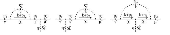
Figure 3: The diagrams for $\tau^{-}\to\mu^{-}\left(S_{b}^{0}\right)^{*}$.

Decays of charged leptons which are unsuppressed by $1/m_{R}$ are [35] $\mu^{-}\to e^{-}e^{+}e^{-}$, $\tau^{-}\to\mu^{-}e^{+}e^{-}$, $\tau^{-}\to\mu^{-}\mu^{+}\mu^{-}$ and $\tau^{-}\to e^{-}e^{+}e^{-}$. In Fig. 3 we have depicted the Feynman diagrams for the vertex $\tau^{-}\to\mu^{-}\left(S_{b}^{0}\right)^{*}$, where $\left(S_{b}^{0}\right)^{*}$ is a virtual neutral scalar; this is the vertex responsible for the amplitude $\mathcal{A}(\tau^{-}\to\mu^{-}\ell^{+}\ell^{-})$ ($\ell=e,\mu$) which does not vanish in the limit $m_{R}\to\infty$. Also the flavour-changing scalar decays of the type $S_{b}^{0}\to e^{+}\mu^{-}$ are unsuppressed. On the other hand, the decay amplitudes for $\tau^{-}\to\mu^{-}\mu^{-}e^{+}$ and $\tau^{-}\to e^{-}e^{-}\mu^{+}$ stem from box diagrams and behave like $1/m_{R}^{2}$ for large $m_{R}$. The amplitudes for $\mu\to e\gamma$ and $Z\to e^{-}\mu^{+}$ have the same behaviour.

While the processes whose amplitudes are suppressed by $1/m_{R}^{2}$ are completely invisible for all practical purposes, the decay rate of $\mu^{-}\to e^{-}e^{+}e^{-}$, although its amplitude is small because it contains a product of four Yukawa couplings, could eventually be within experimental reach.

Acknowledgments: The author thanks the organizers for the invitation, the pleasant and stimulating atmosphere and for choosing such a nice place for the school.

References

-
[1]
S.M. Bilenky and S.T. Petcov,
Massive neutrinos and neutrino oscillations,
Rev. Mod. Phys. 59 (1987) 671;
K. Zuber, On the physics of massive neutrinos, Phys. Rept. 305 (1999) 295 [9811267];
S.M. Bilenky, C. Giunti and W. Grimus, Phenomenology of neutrino oscillations, Prog. Part. Nucl. Phys. 43 (1999) 1 [hep-ph/9812360];
M. Gonzalez-Garcia and Y. Nir, Neutrino masses and mixing: Evidence and implications, Rev. Mod. Phys. 75 (2003) 345 [hep-ph/0202058];
V. Barger, D. Marfatia and K. Whisnant, Progress in the physics of massive neutrinos, Int. J. Mod. Phys. E 12 (2003) 569 [hep-ph/0308123];
A.Yu. Smirnov, Neutrino physics: Open questions, Int. J. Mod. Phys. A 19 (2004) 1180 [hep-ph/0311259]. -
[2]
G. Altarelli and F. Feruglio,
Models of neutrino masses and mixings,
New J. Phys. 6 (2004) 106
[hep-ph/0405048];
A.S. Joshipura, Summary of model predictions for , Proceedings of the 5th Workshop on Neutrino Oscillations and their Origin (NOON2004), Tokyo, Japan, 11–15 Feb. 2004, p. 187 [hep-ph/0411154];
G. Altarelli, Normal and special models of neutrino masses and mixings, to be published in the Proceedings of 19th Rencontres de physique de la vallée d’Aoste: Results and perspectives in particle physics, La Thuile, Aosta valley, Italy, 27 Feb.–5 Mar. 2005, hep-ph/0508053;
R.N. Mohapatra et al., Theory of neutrinos: A white paper, hep-ph/0510213;
G. Altarelli, Models of neutrino masses and mixings, Lectures given at the 61st Scottish Universities Summer School in Physics, St. Andrews, Scotland, 8–23 August 2006, [hep-ph/0611117]. - [3] W. Grimus, Neutrino Physics – Theory, Lect. Notes Phys. 629 (2004) 169 [hep-ph/0307149].
-
[4]
M. Maltoni, T. Schwetz, M. Tórtola and J.W.F. Valle,
Status of global fits to neutrino oscillations,
New J. Phys. 6 (2004) 122
[hep-ph/0405172];
G.L. Fogli, E. Lisi, A. Marrone and A. Palazzo, Global analysis of three-flavor neutrino masses and mixings, Prog. Part. Nucl. Phys. 57 (2006) 742 [hep-ph/0506083];
T. Schwetz, Global fits to neutrino oscillation data, Phys. Scripta T127 (2006) 1 [hep-ph/0606060]. -
[5]
F. Wilczek and A. Zee,
Discrete flavor symmetries and a formula for the Cabibbo
angle,
Phys. Lett. B 70 (1977) 418
[Err. ibid. B 72 (1978) 504];
H. Fritzsch, Calculating the Cabibbo angle, Phys. Lett. B 70 (1977) 436. -
[6]
I. Schur,
Ein Satz ueber quadratische Formen mit komplexen
Koeffizienten,
Am. J. Math. 67 (1945) 472;
B. Zumino, Normal forms of complex matrices, J. Math. Phys. 3 (1962) 1055. - [7] W.-M. Yao et al., Review of particle physics, J. Phys. G: Nucl. Part. Phys. 33 (2006) 1.
- [8] R.N. Mohapatra and P. Pal, Massive neutrinos in physics and astrophysics (World Scientific, Singapore, 1991).
-
[9]
J. Schechter and J.W.F. Valle,
Neutrino masses in theories,
Phys. Rev. D 22 (1980) 2227;
S.M. Bilenky, J. Hošek and S.T. Petcov, On oscillations of neutrinos with Dirac and Majorana masses, Phys. Lett. B 94 (1980) 495;
I.Yu. Kobzarev, B.V. Martemyanov, L.B. Okun and M.G. Shchepkin, The phenomenology of neutrino oscillations, Yad. Phys. 32 (1980) 1590 [Sov. J. Nucl. Phys. 32 (1981) 823]. -
[10]
P. Minkowski,
at a rate of one out of muon decays?,
Phys. Lett. B 67 (1977) 421;
T. Yanagida, in Proceedings of the workshop on unified theory and baryon number in the universe, O. Sawata and A. Sugamoto eds., KEK report 79-18, Tsukuba, Japan 1979;
S.L. Glashow, in Quarks and leptons, proceedings of the advanced study institute (Cargèse, Corsica, 1979), J.-L. Basdevant et al. eds., Plenum, New York 1981;
M. Gell-Mann, P. Ramond and R. Slansky, Complex spinors and unified theories, in Supergravity, D.Z. Freedman and F. van Nieuwenhuizen eds., North Holland, Amsterdam 1979;
R.N. Mohapatra and G. Senjanovic, Neutrino mass and spontaneous parity violation, Phys. Rev. Lett. 44 (1980) 912. - [11] W. Grimus and L. Lavoura, The seesaw mechanism at arbitrary order: disentangling the small scale from the large scale, JHEP 11 (2000) 042 [hep-ph/0008179].
- [12] J. Schechter and J.W.F. Valle, Neutrino decay and spontaneous violation of lepton number, Phys. Rev. D 25 (1982) 774.
-
[13]
B. Bajc, A. Melfo, G. Senjanović, F. Vissani,
Fermion mass relations in a supersymmetric theory,
Phys. Lett. B 634 (2006) 272
[hep-ph/0511352];
C.S. Aulakh, S.K. Garg, MSGUT: From bloom to doom, Nucl. Phys. B 757 (2006) 47 [hep-ph/0512224];
S. Bertolini, T. Schwetz, M. Malinský, Fermion masses and mixing in models and the neutrino challenge to supersymmetric grand unified theories, Phys. Rev. D 73 (2006) 115012 [hep-ph/0605006]. - [14] W. Konetschny and W. Kummer, Non-conservation of total lepton number with scalar bosons, Phys. Lett. B 70 (1977) 433.
- [15] A. Zee, A theory of lepton number violation, neutrino Majorana mass, and oscillation, Phys. Lett. B 93 (1980) 389 [Err. ibid. B 110 (1982) 501].
- [16] A. Zee, Charged scalar field and quantum number violation, Phys. Lett. B 161 (1985) 141.
- [17] L. Wolfenstein, A theoretical pattern for neutrino oscillations, Nucl. Phys. B 175 (1980) 93.
-
[18]
C. Jarlskog, M. Matsuda, S. Skadhauge and M. Tanimoto,
Zee mass matrix and bi-maximal neutrino mixing,
Phys. Lett. B 449 (1999) 240
[hep-ph/9812282];
P.H. Frampton and S.L. Glashow, Can the Zee ansatz for neutrino masses be correct?, Phys. Lett. B 461 (1999) 95 [hep-ph/9906375];
Y. Koide, Can the Zee model explain the observed neutrino data?, Phys. Rev. D 64 (2001) 077301 [hep-ph/0104226]. - [19] K.R.S. Balaji, W. Grimus and T. Schwetz, The solar LMA neutrino oscillation solution in the Zee model, Phys. Lett. B 508 (2001) 301 [hep-ph/0104035].
- [20] K.S. Babu, A model of ‘calculable’ Majorana neutrino masses, Phys. Lett. B 203 (1988) 132.
- [21] K.S. Babu and C. Macesanu, Two-neutrino mass generation and its experimental consequences, Phys. Rev. D 67 (2003) 073010 [hep-ph/0212058].
- [22] G.B. Gelmini and M. Roncadelli, Left-handed neutrino mass scale and spontaneously broken lepton number, Phys. Lett. B 99 (1981) 411.
- [23] J. Erler and P. Langacker, Constraints on extended neutral gauge structures, Phys. Lett. B 456 (1999) 68 [hep-ph/9903476].
-
[24]
J. Schechter and J.W.F. Valle,
Neutrino masses in theories,
Phys. Rev. D 22 (1980) 2227;
G. Lazarides, Q. Shafi and C. Wetterich, Proton lifetime and fermion masses in an model, Nucl. Phys. B 181 (1981) 287;
R.N. Mohapatra and G. Senjanović, Neutrino masses and mixings in gauge models with spontaneous parity violation, Phys. Rev. D 23 (1981) 165. - [25] E. Ma and U. Sarkar, Neutrino masses and leptogenesis with heavy Higgs triplets, Phys. Rev. Lett. 80 (1998) 5716 [hep-ph/9802445].
- [26] W. Grimus and L. Lavoura, One-loop corrections to the seesaw mechanism in the multi-Higgs-doublet standard model, Phys. Lett. B 546 (2002) 86 [hep-ph/0207229].
-
[27]
T. Fukuyama and H. Nishiura,
Mass matrix of Majorana neutrinos,
hep-ph/9702253;
R.N. Mohapatra and S. Nussinov, Bimaximal neutrino mixing and neutrino mass matrix, Phys. Rev. D 60 (1999) 013002 [hep-ph/9809415];
E. Ma and M. Raidal, Neutrino mass, muon anomalous magnetic moment, and lepton flavor nonconservation, Phys. Rev. Lett. 87 (2001) 011802 [Err. ibid. 87 (2001) 159901] [hep-ph/0102255];
C.S. Lam, A 2–3 symmetry in neutrino oscillations, Phys. Lett. B 507 (2001) 214 [hep-ph/0104116];
E. Ma, The all-purpose neutrino mass matrix, Phys. Rev. D 66 (2002) 117301 [hep-ph/0207352]. -
[28]
W. Grimus and L. Lavoura,
Softly broken lepton numbers and maximal neutrino mixing,
JHEP 07 (2001) 045
[hep-ph/0105212];
W. Grimus and L. Lavoura, Softly broken lepton numbers: an approach to maximal neutrino mixing, Acta Phys. Polon. B 32 (2001) 3719 [hep-ph/0110041]. - [29] W. Grimus and L. Lavoura, Models of maximal atmospheric neutrino mixing, Acta Phys. Polon. B 34 (2003) 5393 [hep-ph/0310050].
- [30] W. Grimus, A.S. Joshipura, S. Kaneko, L. Lavoura, H. Sawanka and M. Tanimoto, Non-vanishing and from a broken symmetry, Nucl. Phys. B 713 (2005) 151 [hep-ph/0408123].
- [31] P.F. Harrison and W.G. Scott, – reflection symmetry in lepton mixing and neutrino oscillations, Phys. Lett. B 547 (2002) 219 [hep-ph/0210197].
- [32] W. Grimus and L. Lavoura, Renormalization of the neutrino mass operators in the multi-Higgs-doublet standard model, Eur. Phys. J. C 39 (2005) 219 [hep-ph/0409231].
- [33] W. Grimus and L. Lavoura, Maximal atmospheric neutrino mixing in an model, Eur. Phys. J. C 28 (2003) 123 [hep-ph/0211334].
- [34] W. Grimus and L. Lavoura, Maximal atmospheric neutrino mixing and the small ratio of muon to tau mass, J. Phys. G 30 (2004) 73 [hep-ph/0309050].
- [35] W. Grimus and L. Lavoura, Soft lepton-flavor violation in a multi-Higgs-doublet seesaw model, Phys. Rev. D 66 (2002) 014016 [hep-ph/0204070].