Abstract

The anomaly of a discrete symmetry is defined as the Jacobian of the path-integral measure. Assuming that the anomaly at low energies is cancelled by the Green-Schwarz (GS) mechanism at a fundamental scale, we investigate possible Kac-Moody levels for anomalous discrete family symmetries. As the first example, we consider discrete abelian baryon number and lepton number symmetries in the minimal supersymmetric standard model with the see-saw mechanism, and we find that the ordinary unification of gauge couplings is inconsistent with the GS conditions, indicating the possible existence of further Higgs doublets. We consider various recently proposed supersymmetric models with a non-abelian discrete family symmetry. In a supersymmetric example with $Q_{6}$ family symmetry, the GS conditions are such that the gauge coupling unification appears close to the Planck scale.

1 Introduction

Though the standard model (SM) is very successful, it possesses many unsatisfactory features. One of them is the redundancy of the free parameters in the Yukawa sector. There exist (infinitely) many physically equivalent Yukawa matrices that can produce the same physical quantities, such as the fermion masses and mixings. Since there is no principle to fix the Yukawa structure in the SM, the SM must be extended to impose a family symmetry in order to reduce the redundancy of the parameters. Recently, non-abelian discrete symmetries have been used to extend the SM.[1, 2, 3, 4, 5, 6, 7]

Another unsatisfactory feature of the SM is the fine-tuning problem of the Higgs mass, which can be softened by supersymmetry (SUSY). Moreover, successful gauge coupling unification in the minimal supersymmetric standard model (MSSM) seems to support the existence of low-energy SUSY. However, the situation is not this simple, because SUSY is broken at low energies. It is widely believed that to maintain the nice renormalization property of a supersymmetric theory, SUSY must be broken softly. It is known that there are more than one hundred soft breaking terms and, unless they are fine-tuned, they create large flavor changing neutral currents (FCNC) and CP violations. Fortunately, however, this SUSY flavor problem can be softened by a non-abelian family symmetry.[8]

The above cited facts suggest that a family symmetry could cure certain pathologies of the SM and MSSM. This leads us to conjecture that a family symmetry consistent at low energies is a remnant of a symmetry of a more fundamental theory. If this is the case, the symmetry should be anomaly-free, at least at a fundamental scale. This provides the motivation to investigate anomalies of the discrete family symmetries of recently proposed models. In this paper, we assume that the anomaly of a discrete symmetry at low energies is canceled by the Green-Schwarz (GS) mechanism [9, 10, 11] at a more fundamental scale. In this scenario, the Kac-Moody $k_{i}$ levels play an important role, and if the Kac-Moody levels assume non-trivial values, the GS cancellation conditions of anomalies modify the ordinary unification of gauge couplings. Note that it is impossible to construct a realistic, renormalizable model with a low-energy non-abelian discrete family symmetry in the case of the minimal content of the $SU(2)_{L}$ Higgs fields. However, an extension of the Higgs sector may spoil the successful gauge coupling unification of the MSSM. Therefore, a possible change of the ordinary unification condition because of the existence of nontrivial Kac-Moody $k_{i}$ levels is consistent with the assumption regarding the existence of a low-energy non-abelian discrete family symmetry.

The anomalies of discrete symmetries have been studied in Refs. [12, 13, 14, 15]. In those papers, it is assumed that all discrete symmetries at low energies are gauged at high energies, as in the case of Ref. [16]. In other words, it is assumed that to survive quantum gravity effects, such as wormholes,[17]  all low-energy discrete symmetries must be generated from a spontaneous breakdown of continuous gauge symmetries.

In §2, using Fujikawa’s method, [18]  we calculate the Jacobian of the path-integral measure of an anomalous abelian discrete symmetry. We do this to recall and to demonstrate that the Jacobian can be calculated for a finite discrete transformation parameter. In §3, we use the result of §2 to calculate the Jacobian for a non-abelian discrete transformation. Anomaly cancellation is studied in §5. First we recall the case of an anomalous $U(1)$, and then we extend the cancellation mechanism to the case of discrete symmetries. In contrast to the treatment of Ref. [14], we do not assume that the discrete symmetry in question is not a remnant of a spontaneously broken continuous symmetry. As the first example, we consider discrete abelian baryon number and lepton number symmetries in the minimal supersymmetric standard model with the see-saw mechanism in §6. We find that the GS cancellation conditions can be satisfied if $k_{3}/k_{2}=\mbox{even}/\mbox{odd}$. This implies that the ordinary unification of gauge couplings is inconsistent with the GS conditions, indicating the possible existence of further Higgs doublets. We investigate the unification of gauge couplings for $k_{3}/k_{2}=2$ and find that the unification scale appears close to the Planck scale for three pairs of $SU(2)_{L}$ doublet Higgs supermultiplets. Recently developed models with $D_{7},A_{4}$ and $Q_{6}$ symmetries are treated in §7, and §8 is devoted to a summary.

2 Anomalies of Abelian discrete symmetries

An anomaly is a violation of a symmetry at the quantum level. In the case of a continuous symmetry, an anomaly implies that the corresponding Noether current is not conserved. For discrete symmetries, however, we cannot define an anomaly in this way, because there are no corresponding Noether currents. However, Fujikawa’s method,[18]  which is based on the calculation of the Jacobian of the path-integral measure, can be used to define the anomalies of discrete symmetries. As we see below, the calculation used in this method is basically the same as that of the conventional method.

Let us start by considering a Yang-Mills theory with massless fermions $\psi$ in Euclidean space-time, which can be described by the following path-integral with the Lagrangian:

$$Z=\int{\cal D}{\bar{\psi}}{\cal D}\psi\ \exp\left[\int d^{4}x{\cal L}\right],$$ (1)

$${\cal L}=i{\bar{\psi}}\ /{D}\psi-\frac{1}{2g^{2}}{\rm Tr}[F^{\mu\nu}F_{\mu\nu}],$$ (2)

$$D_{\mu}=\partial_{\mu}-iA_{\mu},$$ (3)

$$F_{\mu\nu}=\partial_{\mu}A_{\nu}-\partial_{\nu}A_{\mu}-i[A_{\mu}\ A_{\nu}],$$ (4)

$$A_{\mu}\equiv gT^{a}A^{a}_{\mu}\ ,\ \ \ {\rm Tr}[T^{a}T^{b}]=\frac{1}{2}\delta^{ab},$$ (5)

here we have dropped the path-integral measure of the gauge boson $A_{\mu}$, because it does not contribute to the anomaly. Then we carry out the chiral phase rotation

$$\psi\rightarrow\psi^{{}^{\prime}}=e^{i\alpha\gamma_{5}}\psi,$$ (6)

where $\alpha$ is a finite discrete parameter. Under this transformation, the Lagrangian is invariant. Next we consider the transformation properties of the path-integral measure. To this end, we follow Ref. [18] and define the eigenstates $\varphi_{n}(x)$ of $/{D}$, i.e.,

$$/{D}\varphi_{n}(x)=\lambda_{n}\varphi_{n}(x),\hskip 28.45274pt\varphi^{\dagger}_{n}\ /{D}=\lambda_{n}\varphi^{\dagger}_{n}(x),$$ (7)

through the relations

$$\psi_{i}(x)=\sum_{n}a_{n}\varphi_{n,i}(x),\hskip 22.76228pt\bar{\psi_{i}}(x)=\sum_{n}\bar{b}_{n}\varphi^{\dagger}_{n,i}(x),\hskip 17.07182pt$$ (8)

$$\int d^{4}x\ \varphi_{n,i}^{{\dagger}}(x)\varphi_{m,i}(x)=\delta_{nm},$$ (9)

$$\sum_{n}^{\infty}\varphi_{n,i}(x)\varphi_{n,j}^{{\dagger}}(y)=\delta_{ij}\delta^{4}(x-y),$$ (10)

where $i$ and $j$ are spinor indices. The Jacobian of the path-integral measure for the above transformation, which is defined as

$${\cal D}\bar{\psi}{\cal D}\psi\rightarrow{\cal D}\bar{\psi}^{{}^{\prime}}{\cal D}\psi^{{}^{\prime}}=\frac{1}{J}{\cal D}\bar{\psi}{\cal D}\psi,$$ (11)

can be written as

$$J^{-1}=\left\{\det\int d^{4}x\ \varphi_{n,i}^{{\dagger}}(x)\left[e^{i\alpha\gamma_{5}}\right]_{ij}\varphi_{m,j}(x)\right\}^{-2}\equiv[\det\ C_{nm}]^{-2},$$ (12)

where

$$C_{nm} = \int d^{4}x\ \varphi_{n,i}^{{\dagger}}(x)\left[e^{i\alpha\gamma_{5}}\right]_{ij}\varphi_{m,j}(x).$$ (13)

The quantity $C_{nm}$ is defined as the expansion

$$C_{nm} = \delta_{nm}+\int d^{4}x\ \varphi_{n,i}^{{\dagger}}(x)\left[i\alpha\gamma_{5}\right]_{ij}\varphi_{m,j}(x)$$ (14)

$$\ \ \ \ \ \ +\int d^{4}x\ \varphi_{n,i}^{{\dagger}}(x)\frac{1}{2!}\left[i\alpha\gamma_{5}\right]_{ij}^{2}\varphi_{m,j}(x)$$

$$\ \ \ \ \ \ +\int d^{4}x\ \varphi_{n,i}^{{\dagger}}(x)\frac{1}{3!}\left[i\alpha\gamma_{5}\right]_{ij}^{3}\varphi_{m,j}(x)+\cdot\cdot\cdot.$$

To proceed, we first derive the following identity by using the completeness relation given in Eq. (10):

$$\int d^{4}x\ \varphi_{n,i}^{{\dagger}}(x)\left[i\alpha\gamma_{5}\right]_{ij}^{2}\varphi_{m,j}(x)\hskip 199.16928pt$$

$$=\int d^{4}x\int d^{4}y\ \varphi_{n,i}^{{\dagger}}(x)\left[i\alpha\gamma_{5}\right]_{ij}\delta_{jk}\delta^{4}(x-y)\left[i\alpha\gamma_{5}\right]_{kl}\varphi_{m,l}(y)\hskip 7.96674pt$$

$$=\int d^{4}x\int d^{4}y\ \varphi_{n,i}^{{\dagger}}(x)\left[i\alpha\gamma_{5}\right]_{ij}\varphi_{p,j}(x)\varphi_{p,k}^{{\dagger}}(y)\left[i\alpha\gamma_{5}\right]_{kl}\varphi_{m,l}(y)$$

$$=\tilde{C}_{np}\tilde{C}_{pm}=\tilde{C}^{2}_{nm},\hskip 206.28247pt$$ (15)

where

$$\tilde{C}_{nm} = \int d^{4}x\ \varphi_{n,i}^{{\dagger}}(x)\left[i\alpha\gamma_{5}\right]_{ij}\varphi_{m,j}(x).$$ (16)

In a similar manner, we can prove the identity

$$\int d^{4}x\ \varphi_{n,i}^{{\dagger}}(x)\left[i\alpha\gamma_{5}\right]_{ij}^{N}\varphi_{m,j}(x)=\tilde{C}^{N}_{nm}.$$ (17)

Therefore we can rewrite Eq. (14) as

$$\int d^{4}x\ \varphi_{n,i}^{{\dagger}}(x)\left(e^{i\alpha\gamma_{5}}\right)_{ij}\varphi_{m,j}(x) = \delta_{nm}+\tilde{C}_{nm}+\frac{1}{2!}\tilde{C}^{2}_{nm}+\frac{1}{3!}\tilde{C}^{3}_{nm}+\cdots~{}.$$ (18)

Then we use $\det A=\exp\{{\rm Tr}\ln A\}$ to obtain

$$J^{-1} = \det\left\{\int d^{4}x\ \varphi_{n,i}^{{\dagger}}(x)\left(e^{i\alpha\gamma_{5}}\right)_{ij}\varphi_{m,j}(x)\right\}^{-2}\hskip 85.35826pt$$ (19)

$$= \exp\left\{-2\sum_{n}^{\infty}\int d^{4}x\ \varphi_{n,i}^{{\dagger}}(x)\left[i\alpha\gamma_{5}\right]_{ij}\varphi_{n,j}(x)\right\}.$$

Note that in obtaining Eq. (19) we did not assume that the transformation parameter $\alpha$ is infinitesimal.

Next we use the quantity

$$\lim_{\Lambda\rightarrow\infty}e^{-(\lambda_{n}/\Lambda)^{2}}$$ (20)

as a regulator for the divergent summation, and we find

$$J^{-1} = \exp\left\{-2\lim_{\Lambda\rightarrow\infty}\sum_{n}^{\infty}\int d^{4}x\ \varphi_{n,i}^{{\dagger}}(x)[i\alpha\gamma_{5}]_{ij}e^{-(\lambda_{n}/\Lambda)^{2}}\varphi_{n,j}(x)\right\}$$ (21)

$$= \exp\left\{-2i\lim_{\Lambda\rightarrow\infty}{\rm Tr}\int\frac{d^{4}k}{(2\pi)^{4}}\int d^{4}x\ e^{-ikx}\alpha\gamma_{5}e^{-(\not{D}/\Lambda)^{2}}e^{ikx}\right\}$$

$$= \exp\left\{-2i\lim_{\Lambda\rightarrow\infty}{\rm Tr}\int\frac{d^{4}k}{(2\pi)^{4}}\int d^{4}x\ \alpha\gamma_{5}\right.$$

$$\hskip 56.9055pt\times\left.\exp\left\{\frac{1}{\Lambda^{2}}\left[-(ik_{\mu}+D_{\mu})^{2}-\frac{i}{4}[\gamma^{\mu}\ \gamma^{\nu}]F_{\mu\nu}\right]\right\}\right\}.$$

Since we are working in the Euclidean space-time, we have the metric $g^{\mu\nu}={\rm diag}(-1,-1,-1,-1)$. As is well known,[18]  the limiting procedure yields

$$J^{-1}=\exp\left\{-i\int d^{4}x\ \frac{\alpha}{16\pi^{2}}{\rm Tr}\left[\epsilon^{\mu\nu\rho\sigma}F_{\mu\nu}F_{\rho\sigma}\right]\right\}.$$ (22)

In this way we can define anomalies of discrete symmetries.

3 Anomalies of non-Abelian discrete family symmetries

We start with the Lagrangian

$${\cal L}=i\bar{\psi}\ /{D}\psi-\frac{1}{2g^{2}_{L}}{\rm Tr}[F^{\mu\nu}(L)F_{\mu\nu}(L)]-\frac{1}{2g^{2}_{R}}{\rm Tr}[F^{\mu\nu}(R)F_{\mu\nu}(R)],$$ (23)

$$D_{\mu}=\partial_{\mu}-iL_{\mu}^{a}T^{a}_{L}P_{L}-iR_{\mu}^{b}T^{b}_{R}P_{R},$$ (24)

which describes an $SU(N_{L})\times SU(N_{R})$ chiral Yang-Mills theory. Here $L^{a}$ ($R^{a}$) are gauge bosons that couple to the left-handed (right-handed) fermions, and $P_{L}$ and $P_{R}$ are the projection operators on the left-handed and right-handed pieces, respectively. Then we consider the non-abelian discrete chiral transformation

$$\psi_{i,\alpha^{{}^{\prime}}}(x)\rightarrow\psi^{{}^{\prime}}_{i,\alpha}=\left[e^{iXP_{L}+iYP_{R}}\right]_{ij,\alpha\beta}\psi_{j,\beta},$$ (25)

where $X$ and $Y$ are matrices that act on the family indices $\alpha,\beta=1-3$. This transformation is a unitary transformation that does not mix the left-handed and right-handed fields. Accordingly, we define the following phases:

$$e^{i\alpha_{L}}\equiv\det(e^{iX}),\hskip 28.45274pte^{i\alpha_{R}}\equiv\det(e^{iY}),$$ (26)

$$\alpha_{L}\equiv{\rm Tr}(X),\hskip 48.36958pt\alpha_{R}\equiv{\rm Tr}(Y).$$ (27)

In contrast to the previous case, we introduce two complete sets of eigen-states:

$$/{D}^{{\dagger}}\ /{D}\varphi_{n}=\lambda_{n}^{2}\varphi_{n},\hskip 76.82234pt/{D}\ /{D}^{{\dagger}}\phi_{n}=\lambda_{n}^{2}\phi_{n},$$ (28)

$$\psi_{i,\alpha}(x)=\sum_{n}a_{n}\varphi_{n,i,\alpha}(x),\hskip 28.45274pt\bar{\psi}_{i,\alpha}(x)=\sum_{n}\bar{b}_{n}\phi_{n,i,\alpha}^{\dagger}(x).$$ (29)

Using these expressions, we then calculate the Jacobian for the transformation (25), where we denote the Jacobian for ${\cal D}\psi$ by $j$ and that for ${\cal D}\bar{\psi}$ by $\bar{j}$, so that the total Jacobian $J$ is given by $\bar{j}j$. After calculations similar to those in the abelian case, we find

$$j^{-1} = \left\{\det\int d^{4}x\ \varphi_{n,i,\alpha}^{{\dagger}}(x)\left[e^{iXP_{L}+iYP_{R}}\right]_{ij,\alpha\beta}\varphi_{m,j,\beta}(x)\right\}^{-1}$$ (30)

$$= \exp\left\{-i\int d^{4}x\ \varphi_{n,i,\alpha}^{{\dagger}}(x)\left[XP_{L}+YP_{R}\right]_{ij,\alpha\beta}\varphi_{m,j,\beta}(x)\right\}$$

$$= \exp\left\{-i\lim_{\Lambda\rightarrow\infty}{\rm Tr}\int\frac{d^{4}k}{(2\pi)^{4}}\int d^{4}x\ e^{-ikx}\left[XP_{L}+YP_{R}\right]e^{-(\not{D}^{{\dagger}}\not{D}/\Lambda^{2})}e^{ikx}\right\},$$

and

$$\bar{j}^{-1} = \left\{\det\int d^{4}x\ \phi_{n,i,\alpha}^{{\dagger}}(x)\left[e^{-iXP_{R}-iYP_{L}}\right]_{ij,\alpha\beta}\phi_{m,j,\beta}(x)\right\}^{-1}$$ (31)

$$= \exp\left\{i\int d^{4}x\ \phi_{n,i,\alpha}^{{\dagger}}(x)\left[XP_{R}+YP_{L}\right]_{ij,\alpha\beta}\phi_{m,j,\beta}(x)\right\}$$

$$= \exp\left\{i\lim_{\Lambda\rightarrow\infty}{\rm Tr}\int\frac{d^{4}k}{(2\pi)^{4}}\int d^{4}x\ e^{-ikx}\left[XP_{R}+YP_{L}\right]e^{-(\not{D}\not{D}^{{\dagger}}/\Lambda^{2})}e^{ikx}\right\},$$

where ${\rm Tr}$ stands for the trace over the spinor, family and Yang-Mills indices. Carrying out the trace in the family space, we obtain

$$j^{-1}=\exp\left\{-i\lim_{\Lambda\rightarrow\infty}{\rm Tr}\int\frac{d^{4}k}{(2\pi)^{4}}\int d^{4}x\ e^{-ikx}\left[\alpha_{L}P_{L}+\alpha_{R}P_{R}\right]e^{-(\not{D}^{{\dagger}}\not{D}/\Lambda^{2})}e^{ikx}\right\}$$ (32)

where use has been made of Eqs. (26) and (27). In the same way, we obtain a similar expression for $\bar{j}^{-1}$. The rest of the calculations are very similar to those in the previous case, and we finally obtain the total Jacobian,

$$J^{-1} = j^{-1}\bar{j}^{-1}$$ (33)

$$= \exp\left\{i\int d^{4}x\frac{1}{32\pi^{2}}{\rm Tr}\epsilon^{\mu\nu\rho\sigma}\left[\alpha_{L}\ F_{\mu\nu}(L)F_{\rho\sigma}(L)-\alpha_{R}\ F_{\mu\nu}(R)F_{\rho\sigma}(R)\right]\right\},$$

where

$$F_{\mu\nu}(L)=\partial_{\mu}L_{\nu}-\partial_{\nu}L_{\mu}-i[L_{\mu}\ L_{\nu}],$$ (34)

$$F_{\mu\nu}(R)=\partial_{\mu}R_{\nu}-\partial_{\nu}R_{\mu}-i[R_{\mu}\ R_{\nu}].$$ (35)

Here, $\alpha_{R}$ and $\alpha_{L}$ are the phases of the transformation matrices defined in Eq. (26), which need not be continuous nor infinitesimal. These phases correspond to the abelian parts of the non-abelian discrete family transformations. Therefore, to calculate the anomaly of a non-abelian discrete family symmetry, we only have to take into account its abelian parts. We will consider specific examples in the later sections.

4 Pontryagin index

The expression

$$\int d^{4}x\ \frac{1}{32\pi^{2}}{\rm Tr}\left[\epsilon^{\mu\nu\rho\sigma}F_{\mu\nu}F_{\rho\sigma}\right]$$ (36)

in Eq. (33) is called the Pontryagin index, which is an integer $\nu$. For the case $\alpha_{L}\neq 0$ and $\alpha_{R}=0$, for instance, the Jacobian becomes

$$J^{-1}=\exp\{i\alpha_{L}\nu\}.$$ (37)

Since only the abelian parts of a non-abelian discrete family symmetry contribute to the anomalous Jacobian, the phase has the form

$$\alpha_{L}=\sum_{I}~{}(2\pi/N_{I})\sum_{i}q_{I,i},$$ (38)

where we have assumed that the abelian parts can be written as $\Pi_{I=1}Z_{N_{I}}$, and $q_{I,i}$ represents the charge of $Z_{N_{I}}$. Therefore, we obtain $J^{-1}=1$ if the relation

$$\sum_{i}q_{iI,}=rN_{I}\ \ \ (r=0,\pm 1,\pm 2\cdots)$$ (39)

is satisfied for each $I$.

5 Anomaly cancellation and gauge coupling unification

In the previous sections we have seen that anomalies of discrete symmetries can be defined as the anomalous Jacobian of the path-integral measure. In this section, we study how an anomaly can be canceled by the Green-Schwarz (GS) mechanism.[9, 10, 11]  First, we review the GS mechanism for an anomalous $U(1)_{A}$ symmetry, and then we apply the GS mechanism to discrete symmetries.

5.1 Green-Schwarz mechanism

String theory when compactified on four dimensions usually contains anomalous $U(1)$ local symmetries. Consider a supersymmetric Yang-Mills theory based on a gauge group ${\cal G}\otimes U(1)_{A}$, where $U(1)_{A}$ is assumed to be anomalous. The $U(1)_{A}$ gauge transformation is defined as

$$\Phi\rightarrow e^{-i\Lambda}\Phi,$$ (40)

$$V_{A}\rightarrow V_{A}+i(\Lambda-\bar{\Lambda}),\hskip 28.45274pt$$ (41)

where $\Phi$ and $\Lambda$ are chiral supermultiplets and $V_{A}$ is the vector supermultiplet of $U(1)_{A}$. The anomaly for this transformation is calculated in Ref. [19]. Using the result of Ref. [19], we find that the anomalous Jacobian for the $[{\cal G}]^{2}\times U(1)_{A}$ anomaly, for instance, is given by

$$J^{-1}=\exp\left\{-i{\cal A}\int d^{4}xd^{2}\theta\ {\rm Tr}\left[\Lambda W^{a}W_{a}\right]_{F}\right\},$$ (42)

where ${\cal A}$ is the anomaly coefficient for $[{\cal G}]^{2}\times U(1)_{A}$ and $W$ is the chiral supermultiplet of the gauge supermultiplet corresponding to the gauge group ${\cal G}$. This anomaly is canceled by the gauge kinetic term,

$$k\ {\rm Tr}\left[SW^{a}W_{a}\right]_{F},$$ (43)

if we correspondingly shift the dilaton supermultiplet $S$ as

$$S\rightarrow S^{{}^{\prime}}=S+i\frac{\cal A}{k}\Lambda,$$ (44)

where $k$ is the Kac-Moody level. We must simultaneously modify the transformation property of the dilaton supermultiplet $S$ to restore the invariance of its Kähler potential. At the quantum level, the Kähler potential is modified to include $\delta_{GS}V_{A}$ in the logarithm:

$$K=\ln(S+\bar{S}-\delta_{GS}V_{A}).$$ (45)

Thus, the Kähler potential is invariant if the relation

$$\frac{\cal A}{k}=\delta_{GS}$$ (46)

is satisfied.

In the case ${\cal G}=SU(3)_{C}\otimes SU(2)_{L}\otimes U(1)_{Y}$, there exist various possibilities for the anomaly: $[SU(3)_{C}]^{2}\times U(1)_{A}\$, $\ [SU(2)_{L}]^{2}\times U(1)_{A}\$, $\ [U(1)_{Y}]^{2}\times U(1)_{A}\$,$\ [U(1)_{A}]^{3}\$ and $\ [{\rm gravity}]^{2}\times U(1)_{A}$. If we denote the respective anomaly coefficients by ${\cal A}_{3}$, ${\cal A}_{2}$, ${\cal A}_{1}$, ${\cal A}_{A}$, and ${\cal A}_{G}$, then the anomaly cancellation conditions are given by

$$\frac{{\cal A}_{3}}{k_{3}}=\frac{{\cal A}_{2}}{k_{2}}=\frac{{\cal A}_{1}}{k_{1}}=\frac{{\cal A}_{A}}{k_{A}}=\frac{{\cal A}_{G}}{12}=\delta_{GS}.$$ (47)

Note that the Kac-Moody levels of a non-abelian group are positive integers, while there is no restriction on the Kac-Moody levels for an abelian group.

5.2 Gauge coupling unification

Next we consider the above discussion in terms of the component fields to determine the relation of the Kac-Moody levels to the gauge coupling unification. To this end, we define $S|_{\theta=\bar{\theta}=0}=\varphi+i\eta\$ and $\ \Lambda|_{\theta=\bar{\theta}=0}=\phi+i\xi$. For the axion field $\eta$, the shift (44) corresponds to

$$\eta\rightarrow\eta^{{}^{\prime}}=\eta+\phi\delta_{GS},$$ (48)

and the VEV of the dilaton field $\varphi$ is merely the string coupling, i.e.,

$$\langle\varphi\rangle=\frac{1}{g^{2}_{st}}.$$ (49)

Also, the gauge couplings $g_{i}$ are related to the string coupling according to

$$\frac{k_{i}}{g^{2}_{st}}=\frac{1}{g^{2}_{i}}.$$ (50)

Therefore, the conditions for the gauge coupling unification of the SM gauge couplings can be written as

$$k_{3}g_{3}^{2}=k_{2}g_{2}^{2}=k_{1}g_{1}^{2}=g^{2}_{st}$$ (51)

at the string scale. It is therefore clear that the anomaly cancellation conditions (47) have a non-trivial influence on the gauge coupling unification.

5.3 The GS mechanism for discrete symmetries

Here we extend the GS mechanism to the case of discrete symmetries. Unlike Ref. [14], we do not assume that the discrete symmetry in question arises from a spontaneous breakdown of a continuous local symmetry. We instead assume that the anomalous discrete symmetry at low energies is a remnant of an anomaly-free discrete symmetry, and that its low energy anomaly is cancelled by the GS mechanism at a more fundamental scale. In superstring theory when compctified on a six-dimensional Calabi-Yau manifold, for instance, there indeed exist certain non-abelian discrete symmetries.[21]

We consider the $Z_{N}$ transformation

$$\Phi\rightarrow e^{-i\alpha}\Phi,$$ (52)

$$V\rightarrow V\hskip 48.36958pt$$

in a supersymmetric gauge theory in order to determine how to cancel the anomaly. As in the previous case, the transformation parameter $\alpha$ is discrete, i.e. $\alpha=\frac{2\pi}{N}$, and $V$ is the vector supermultiplet of the gauge group. The anomaly of this transformation has the same form as (42):

$$J^{-1}=\exp\left\{-i{\cal A}\int d^{4}xd^{2}\theta\ {\rm Tr}\left[\alpha W^{a}W_{a}\right]_{F}\right\},$$ (53)

which is also canceled by the gauge kinetic term. In this case, however, the dilaton supermultiplet must be shifted by only a constant amount $\alpha$, i.e.,

$$S\rightarrow S^{{}^{\prime}}=S+i\frac{\cal A}{k}\alpha,$$ (54)

for the cancellation mechanism to work. This means that because $\alpha$ is a constant, independent of $x$ and $\theta$, only the imaginary part of the scalar component of $S$, which is the axion field, should be shifted. Note that the Kähler potential (45) does not depend on $\delta_{GS}$ because the vector supermultiplet does not change under the transformation Eq. (52). Therefore, the anomaly cancellation conditions for the SM gauge group are

$$\frac{{\cal A}_{3}}{k_{3}}=\frac{{\cal A}_{2}}{k_{2}}=\frac{{\cal A}_{1}}{k_{1}}=\frac{{\cal A}_{G}}{12},$$ (55)

where ${\cal A}_{3}$, ${\cal A}_{2}$, ${\cal A}_{1}$ and ${\cal A}_{G}$ are the anomaly coefficients of the anomalies $[SU(3)_{C}]^{2}\times Z_{N}\$, $\ [SU(2)_{L}]^{2}\times Z_{N}\$, $\ [U(1)_{Y}]^{2}\times Z_{N}\$ and $\ [{\rm gravity}]^{2}\times Z_{N}$, respectively. Because the $\ [U(1)_{Y}]^{2}\times Z_{N}\$ anomaly does not yield useful constraints on the low-energy effective theory, and we cannot calculate ${\cal A}_{G}$ for the low-energy effective theory, we do not consider them when studying models in the next section. However, massive Majorana fields can contribute to ${\cal A}_{2}$ and ${\cal A}_{3}$ for even $N$, because Majorana masses are allowed by the discrete symmetry if the Majorana fields belong to real representations of $SU(2)_{L}$ and $SU(3)_{C}$.[14]  Taking into account the contributions from the massive fields, we arrive at the anomaly cancellation conditions[14]

$$\frac{{\cal A}_{3}+\frac{pN}{2}}{k_{3}}=\frac{{\cal A}_{2}+\frac{qN}{2}}{k_{2}},$$ (56)

with integer $p$ and $q$, where $pN/2$ and $qN/2$ take into account the possible contributions from the heavy fields.

In this section, we have applied the GS mechanism to an abelian discrete symmetry. In §7, we consider anomaly cancellation of a non-abelian discrete family symmetry. As we have seen in §3, however, only the abelian parts contribute to the anomaly, even if we consider a non-abelian discrete family symmetry. Hence, Eq. (56) can also be applied to the case of a non-abelian discrete family symmetries.

6 Anomalies of accidental $Z_{N}$ symmetries

As an example of anomaly cancellation for discrete symmetries, let us consider the baryon and lepton number symmetries in the MSSM with R-parity, in which the see-saw mechanism is implemented to generate neutrino masses. The baryon number $U(1)_{B}$ is conserved at the classical level, while the lepton number $U(1)_{L}$ is not conserved because of the Majorana masses of the right-handed neutrinos. However, its abelian discrete subgroups, $(Z_{N})_{L}$ with even $N$, are intact at the classical level. In the following discussion, we first investigate anomalies and their GS cancellation conditions for abelian discrete subgroups $(Z_{M})_{B}$ of $U(1)_{B}$ and $(Z_{N})_{L}$. Then we study how the GS cancellation conditions influence gauge coupling unification. The $(Z_{N})_{L}$ and $(Z_{M})_{B}$ charges of the supermultiplets of the MSSM are given in Table 1.

Table 1: The $(Z_{N})_{L}$ and $(Z_{N})_{B}$ charges. $N$ is even and $a,b,c,\cdots p=0,1,2\cdots$.

	$Q$	$U^{c}$	$D^{c}$	$L$	$E^{c}$	$\nu_{R}$	$H^{u}$	$H^{d}$
$(Z_{N})_{L}$	$aN$	$bN$	$cN$	$\frac{N}{2}+dN$	$\frac{N}{2}+eN$	$\frac{N}{2}+fN$	$gN$	$hN$
$(Z_{M})_{B}$	$B+iM$	$-B+jM$	$-B+kM$	$lM$	$mM$	$nM$	$oM$	$pM$

The anomaly coefficients for $(Z_{N})_{L}$ are found to be

$$2{\cal A}_{3}=\frac{N}{2}[12a+6b+6c],$$ (57)

$$2{\cal A}_{2}=\frac{N}{2}[18a+3+6d+2g+2h].$$ (58)

Therefore, the GS cancellation conditions become

$$\frac{k_{3}}{k_{2}}=\frac{12a+6b+6c}{18a+3+6d+2g+2h}=\frac{\rm even}{\rm odd}.$$ (59)

Note that $k_{3}=k_{2}=1$ is not a solution. In a similar way, we can calculate the anomaly coefficients for $(Z_{M})_{B}$, and we find

$$\frac{k_{3}}{k_{2}}=\frac{9B+(9i+3\ell+o+p)M}{(6i+3j+3k)M}=\frac{{\rm even}\ {\bf or}\ {\rm odd}}{{\rm even}\ {\bf or}\ {\rm odd}}.$$ (60)

As it is believed to be difficult to build realistic models with higher Kac-Moody levels in string theory, we seek solutions to (59) and (60) with lower levels. The solution with the lowest levels that satisfy the conditions (59) and (60) simultaneously is $k_{3}=2,k_{2}=1$, which yields the gauge coupling unification conditions

$$2g_{3}^{2}=g_{2}^{2}=k_{1}g_{1}^{2}=g_{st}^{2},$$ (61)

where $k_{1}$ is arbitrary. Figure 2 plots the ratios $g_{2}^{2}/g_{1}^{2}$ (upper curves) and $g_{2}^{2}/g_{3}^{2}$ (lower curves) as functions of the energy scale. The solid curves correspond to the case with one pair of $SU(2)_{L}$ doublet Higgs supermultiplets, the dotted curves to the case with two pairs, and the dashed curves to the case with three pairs. (We denote the number of the Higgs pairs by $H_{\rm higgs}$.) We see from Figure 2 that the ratio $g_{2}^{2}/g_{3}^{2}$ with $H_{\rm higgs}=3$ becomes close to $2$ at the Planck scale, $M_{PL}=1.2\times 10^{18}$ GeV. For $H_{\rm higgs}=1$ and $2$ there is no chance for the ratio to become close to $2$ below or near $M_{PL}$. In Figure 2 we plot the running of $(\alpha_{1}k_{1})^{-1},(\alpha_{2}k_{2})^{-1}$ and $(\alpha_{3}k_{3})^{-1}$ with $k_{3}=2,k_{2}=1$ and $k_{1}=2.25$ in the case $H_{\rm higgs}=3$. As we have seen above, the GS cancellation conditions of anomalies have a nontrivial influence on the gauge coupling unification, and hence the number of Higgs supermultiplets.

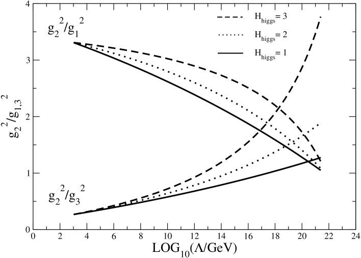
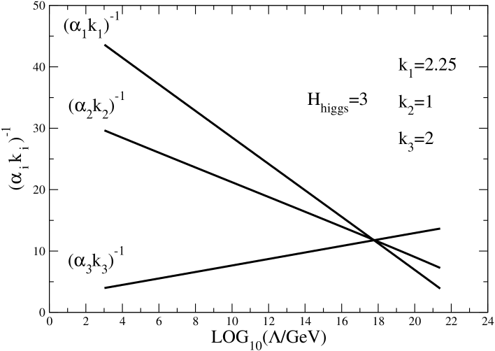
Figure 1: The ratios $g_{2}^{2}/g_{1}^{2}$ (upper curves) and $g_{2}^{2}/g_{3}^{2}$ (lower curves) as functions of the energy scale. The solid curves correspond to the MSSM+$\nu_{R}$ case, the dotted curves to the case with $H_{\rm higgs}=2$, and the dashed curves to the case with $H_{\rm higgs}=3$.

Figure 2: The running of $(\alpha_{1}k_{1})^{-1}$, $(\alpha_{2}k_{2})^{-1}$ and $(\alpha_{3}k_{3})^{-1}$ with $k_{3}=2,k_{2}=1$ and $k_{1}=2.25$ in the case with $H_{\rm higgs}=3$. The unification scale is $10^{18}$ GeV.

7 Models

Recently, a number of models with a non-abelian discrete family symmetry have been proposed.[1, 2, 3, 4, 5, 6, 7]  However, if only the SM Higgs or the MSSM Higgs are present within the framework of renormalizable models, any low-energy non-abelian family symmetry should be hardly broken to be consistent with experimental observations. That is, if a non-abelian discrete family symmetry should be at most softly broken, we need several pairs of $SU(2)_{L}$ doublet Higgs fields. This implies that the conditions of the ordinary unification of gauge couplings, i.e. $k_{2}=k_{3}=k_{1}(3/5)$, cannot be satisfied if we require a low-energy non-abelian discrete family symmetry. Fortunately, however, as we have seen, there is a possibility to satisfy the gauge coupling unification conditions with non-minimal Higgs content if the Kac-Moody levels assume non-trivial values. These Kac-Moody levels also play an important role in the anomaly cancellation (GS mechanism). In the following subsections, we calculate the anomalies of non-abelian discrete family symmetries for recently proposed models and investigate the gauge coupling unification conditions.

7.1 $D_{7}$ model

Let us first calculate the anomaly of the supersymmetric $D_{7}$ model.[5, 6]  $D_{7}$ has fourteen elements and five irreducible representations $({\bf 1,1^{{}^{\prime}},2,2^{{}^{\prime}},2^{{}^{\prime\prime}}})$. This model uses the complex representation,[20]  and thus the character table and the two-dimensional representation matrices of ${\bf 2}$ are as follows:

Table 2: Character table of $D_{7}$.                    

class	n	h	$\chi_{1}$	$\chi_{1^{{}^{\prime}}}$	$\chi_{2}$	$\chi_{2^{{}^{\prime}}}$	$\chi_{2^{{}^{\prime\prime}}}$
$C_{1}$	1	1	1	1	2	2	2
$C_{2}$	7	2	1	$-1$	0	0	0
$C_{3}$	2	7	1	1	$a_{1}$	$a_{2}$	$a_{3}$
$C_{4}$	2	7	1	1	$a_{2}$	$a_{3}$	$a_{1}$
$C_{5}$	2	7	1	1	$a_{3}$	$a_{1}$	$a_{2}$

$a_{k}=2\cos(\frac{2\pi}{7}k)$

$$C_{1}:\left(\begin{array}[]{cc}1&0\\ 0&1\end{array}\right),$$ (64)

$$C_{2}:\left(\begin{array}[]{cc}0&\omega^{k}\\ \omega^{7-k}&0\end{array}\right)\ \ k=0-6\ \ \ \omega=\exp(2\pi i/7),$$ (67)

$$C_{3}:\left(\begin{array}[]{cc}\omega^{6}&0\\ 0&\omega\end{array}\right),\left(\begin{array}[]{cc}\omega&0\\ 0&\omega^{6}\end{array}\right),$$ (72)

$$C_{4}:\left(\begin{array}[]{cc}\omega^{5}&0\\ 0&\omega^{2}\end{array}\right),\left(\begin{array}[]{cc}\omega^{2}&0\\ 0&\omega^{5}\end{array}\right),$$ (77)

$$C_{3}:\left(\begin{array}[]{cc}\omega^{4}&0\\ 0&\omega^{3}\end{array}\right),\left(\begin{array}[]{cc}\omega^{3}&0\\ 0&\omega^{4}\end{array}\right).$$ (82)

The representation matrices for ${\bf 2^{{}^{\prime}}}$ and ${\bf 2^{{}^{\prime\prime}}}$ are obtained from the cyclic rotation of $C_{3}$, $C_{4}$ and $C_{5}$. $D_{7}$ has five kinds of transformation properties, corresponding to five classes. However, the transformation of $C_{1}$ is the identity, and there is no difference among $C_{3}-C_{5}$ when we calculate the anomaly. Hence we consider only $C_{2}$ and $C_{3}$. Under $C_{2}$ and $C_{3}$, the irreducible representations transform as

$$C_{2}\hskip 147.95424ptC_{3}\hskip 76.82234pt$$

$$\begin{array}[]{llllll}{\bf 2}&&\rightarrow\left(\begin{array}[]{cc}0&\omega^{k}\\ \omega^{7-k}&0\end{array}\right){\bf 2}&&&\rightarrow\left(\begin{array}[]{cc}\omega^{6}&0\\ 0&\omega^{1}\end{array}\right),\left(\begin{array}[]{cc}\omega^{1}&0\\ 0&\omega^{6}\end{array}\right){\bf 2},\\ {\bf 2}^{{}^{\prime}}&&\rightarrow\left(\begin{array}[]{cc}0&\omega^{k}\\ \omega^{7-k}&0\end{array}\right){\bf 2}^{{}^{\prime}}&&&\rightarrow\left(\begin{array}[]{cc}\omega^{5}&0\\ 0&\omega^{2}\end{array}\right),\left(\begin{array}[]{cc}\omega^{2}&0\\ 0&\omega^{5}\end{array}\right){\bf 2}^{{}^{\prime}},\\ {\bf 2}^{{}^{\prime\prime}}&&\rightarrow\left(\begin{array}[]{cc}0&\omega^{k}\\ \omega^{7-k}&0\end{array}\right){\bf 2}^{{}^{\prime\prime}}&&&\rightarrow\left(\begin{array}[]{cc}\omega^{4}&0\\ 0&\omega^{3}\end{array}\right),\left(\begin{array}[]{cc}\omega^{3}&0\\ 0&\omega^{4}\end{array}\right){\bf 2}^{{}^{\prime\prime}},\\ {\bf 1}&&\rightarrow{\bf 1}&&&\rightarrow{\bf 1},\\ {\bf 1}^{{}^{\prime}}&&\rightarrow e^{i\frac{2\pi}{2}1}\ {\bf 1}^{{}^{\prime}}&&&\rightarrow{\bf 1}^{{}^{\prime}},\end{array}$$ (106)

where $k=1-7$ and $\omega=\exp(2\pi i/7)$. As mentioned in §3, even if we calculate the anomaly of a non-abelian discrete family symmetry, only the abelian parts contribute to the anomaly. From Eqs. (82) and (106), it is clear that the abelian parts of the $C_{2}$ and $C_{3}$ transformations are $Z_{2}$ and $Z_{7}$, respectively.

The authors of Refs. [5] and [6] introduce into this model the $SU(2)_{L}$ triplet extra Higgs supermultiplets $\xi_{i}$, which have lepton numbers, and assume that all Higgs supermultiplets have generation as well as fermions. The assignment of the $D_{7}$ representations for each matter supermultiplet is presented in Table 3.

Table 3: $D_{7}$ assignment of the matter supermultiplets.

	$Q_{1,2}\ D^{c}_{1,2}$	$U^{c}_{1,2}$	$L_{2,3}\ E^{c}_{2,3}$	$Q_{3}\ D^{c}_{3}\ U^{c}_{3}\ L_{1}\ E^{c}_{1}$	$H^{d}_{1,2}$	$H^{u}_{1,2}$	$\xi_{2,3}$	$H^{d}_{3}\ H^{u}_{3}\ \xi_{1}$
$D_{7}$	2	$2^{{}^{\prime}}$	$2^{{}^{\prime\prime}}$	1	2	$2^{{}^{\prime\prime}}$	$2^{{}^{\prime\prime}}$	1

7.1.1 Computation of anomaly coefficients

Here we compute the anomaly coefficients for the $C_{3}(Z_{7})$ transformations. These transformations have no anomaly, because the determinants of all $C_{3}$ transformation matrices in Eq. (106) are equal to $1$.

Next we compute the anomaly coefficients for the $C_{2}(Z_{2})$ transformations. The first and second generations of $QD^{c}$,$U^{c}$ and $H^{u}H^{d}$ are assigned to ${\bf 2,2^{{}^{\prime}}}$ and ${\bf 2^{{}^{\prime\prime}}}$, respectively, and the third generation is assigned to ${\bf 1}$. Hence, these supermutiplets transform as

$$\Psi_{\alpha=1-3}\rightarrow\left(\begin{array}[]{ccc}0&\omega^{k}&0\\ \omega^{7-k}&0&0\\ 0&0&1\end{array}\right)_{\alpha\beta}\Psi_{\beta=1-3}.$$ (110)

The determinant of this matrix is $\exp(2\pi i/2)=-1$, and therefore these supermultiplets contribute $\frac{2\pi}{2}1$ anomaly coefficients. Here we omit the $Z_{N}$ factor, that is $\frac{2\pi}{N}$, and hence the contributions of these supermultiplets are equal to $1$. The second and third generations of $L,E^{c}$ and $\xi$ are assigned to ${\bf 2^{{}^{\prime\prime}}}$, and the first generation is assigned to ${\bf 1}$. Hence, these supermultiplets transform as

$$\Phi_{\alpha=1-3}\rightarrow\left(\begin{array}[]{ccc}1&0&0\\ 0&0&\omega^{k}\\ 0&\omega^{7-k}&0\end{array}\right)_{\alpha\beta}\Phi_{\beta=1-3},$$ (114)

and contribute $1$ as well. Using these facts, we can compute the anomaly coefficients and find

$$2{\cal A}_{3}=[1\cdot 2+1+1]=4\ ({\rm mod}\ 2),$$ (115)

$$2{\cal A}_{2}=[1\cdot 3+1+1+1]+1\cdot 4\cdot 2=14\ ({\rm mod}\ 2).$$ (116)

Here, we define ${\cal A}_{3}$ and ${\cal A}_{2}$ as the anomaly coefficients of $[SU(3)_{C}]^{2}\times Z_{2}$ and $[SU(2)_{L}]^{2}\times Z_{2}$, respectively. The last term in Eq. (116) is the contribution from the $SU(2)_{L}$ triplet Higgs supermultiplets. As we have seen in §4, these coefficients do not contribute an anomaly. Therefore this model is anomaly-free.

7.2 $A_{4}$ model

As the second example, we calculate the anomaly of the supersymmetric $A_{4}$ model.[1]  $A_{4}$ has twelve elements and four irreducible representations $({\bf 1,1^{{}^{\prime}},1^{{}^{\prime\prime}},3})$. This model also uses the complex representation, and thus the character table and the three-dimensional representation matrices of ${\bf 3}$ are written as follows:

Table 4: Character table of $A_{4}$.             

class	n	h	$\chi_{1}$	$\chi_{1^{\prime}}$	$\chi_{1^{\prime\prime}}$	$\chi_{3}$
$C_{1}$	1	1	1	1	1	3
$C_{2}$	4	3	1	$\omega$	$\omega^{2}$	0
$C_{3}$	4	3	1	$\omega^{2}$	$\omega$	0
$C_{4}$	3	2	1	1	1	$-1$

$\omega=e^{i\frac{2\pi}{3}}$

$$C_{1}:\left(\begin{array}[]{ccc}1&0&0\\ 0&1&0\\ 0&0&1\end{array}\right),$$ (120)

$$C_{2}:\left(\begin{array}[]{ccc}0&0&1\\ 1&0&0\\ 0&1&0\end{array}\right),\left(\begin{array}[]{ccc}0&0&1\\ -1&0&0\\ 0&-1&0\end{array}\right),\left(\begin{array}[]{ccc}0&0&-1\\ -1&0&0\\ 0&1&0\end{array}\right),\left(\begin{array}[]{ccc}0&0&-1\\ 1&0&0\\ 0&-1&0\end{array}\right),$$ (133)

$$C_{3}:\left(\begin{array}[]{ccc}0&1&0\\ 0&0&1\\ 1&0&0\end{array}\right),\left(\begin{array}[]{ccc}0&1&0\\ 0&0&-1\\ -1&0&0\end{array}\right),\left(\begin{array}[]{ccc}0&-1&0\\ 0&0&1\\ -1&0&0\end{array}\right),\left(\begin{array}[]{ccc}0&-1&0\\ 0&0&-1\\ 1&0&0\end{array}\right),$$ (146)

$$C_{4}:\left(\begin{array}[]{ccc}1&0&0\\ 0&-1&0\\ 0&0&-1\end{array}\right),\left(\begin{array}[]{ccc}-1&0&0\\ 0&1&0\\ 0&0&-1\end{array}\right),\left(\begin{array}[]{ccc}-1&0&0\\ 0&-1&0\\ 0&0&1\end{array}\right).$$ (156)

$A_{4}$ has four kinds of transformation properties, corresponding to four classes. However, there is no difference between $C_{2}$ and $C_{3}$ when we calculate the anomaly. The abelian parts of $C_{3}$ and $C_{4}$ are $Z_{3}$ and $Z_{2}$, respectively.

The assignment of the $A_{4}$ representations for the matter supermultiplets is given in Table 5. In addition, the authors of Ref. [1] introduce the extra leptons, quarks and Higgs supermultiplets listed in Table 6.

Table 5: $A_{4}$ assignment of the matter supermultiplets.

	$Q_{1,2,3}\ L_{1,2,3}$	$U^{c}_{1}\ D^{c}_{1}\ E^{c}_{1}$	$U^{c}_{2}\ D^{c}_{2}\ E^{c}_{2}$	$U^{c}_{3}\ D^{c}_{3}\ E^{c}_{3}$	$H^{u}\ H^{d}$
$A_{4}$	3	$1$	$1^{{}^{\prime}}$	$1^{{}^{\prime\prime}}$	1

Table 6: $A_{4}$ and $SU(3)_{C}$ assignments of the extra supermultiplets.

	$u_{1,2,3}\ u^{c}_{1,2,3}$	$d_{1,2,3}\ d^{c}_{1,2,3}$	$e_{1,2,3}\ e^{c}_{1,2,3}$	$N^{c}_{1,2,3}$	$\chi_{1,2,3}$
$A_{4}$	3	3	3	3	3
$SU(3)_{C}$	3	3	1	1	1

7.2.1 Computation of anomaly coefficients

We next compute the anomaly coefficients in the same way as in the case of $D_{7}$. For the $C_{3}(C_{2})$ transformation, the supermultiplets that are assigned to 3 and 1 do not contribute to anomaly, because the determinants of these transformation matrices are equal to 1. Therefore, only ${\bf 1^{{}^{\prime}}}$ and ${\bf 1^{{}^{\prime\prime}}}$ contribute to the anomaly coefficients. As we can see from Table 5, the three generations of the right-handed quark and lepton are assigned to ${\bf 1},{\bf 1^{\prime}{{}^{\prime}}}$ and ${\bf 1^{{}^{\prime\prime\prime}}}$, respectively, and so they transform as

$$1{\rm st}\hskip 14.22636pt{\ddagger}\ \ {\bf 1}\rightarrow{\bf 1},$$ (157)

$$2{\rm nd}\hskip 10.81218pt{\ddagger}\ \ {\bf 1^{{}^{\prime}}}\rightarrow e^{i\frac{2\pi}{3}2}{\bf 1^{{}^{\prime}}},$$ (158)

$$3{\rm rd}\hskip 11.9501pt{\ddagger}\ \ {\bf 1^{{}^{\prime\prime}}}\rightarrow e^{i\frac{2\pi}{3}1}{\bf 1^{{}^{\prime\prime}}}.$$ (159)

Therefore, these representations do not contribute to the anomaly when we take into account all generations.

On the other hand, there is no anomaly for the $C_{4}$ transformation, because all singlets do not transform, and the determinants of all transformation matrices of 3 are equal to 1. Therefore this model is anomaly-free.

7.3 $Q_{6}$ model

We finally calculate the anomaly of the supersymmetric $Q_{6}$ model.[4]  All elements of $Q_{6}$ are constructed from combinations of

$$A_{Q_{6}}=\left(\begin{array}[]{cc}\cos\ \phi_{6}&\sin\ \phi_{6}\\ -\sin\ \phi_{6}&\cos\ \phi_{6}\end{array}\right)_{\phi_{6}=\frac{2\pi}{6}},\hskip 28.45274ptB_{Q}=\left(\begin{array}[]{cc}i&0\\ 0&-i\end{array}\right),$$ (164)

as follows:

$${\cal G}=\{E,A_{Q_{6}},(A_{Q_{6}})^{2},\cdots,(A_{Q_{6}})^{5},B_{Q},A_{Q_{6}}B_{Q},(A_{Q_{6}})^{2}B_{Q},\cdots,(A_{Q_{6}})^{5}B_{Q}\}.$$ (165)

Here, $E$ is the identity element. $Q_{6}$ has six irreducible representations, two doublets and four singlets:

$${\rm doublet} \textdaggerdbl {\bf 2}\ \ \ {\bf 2}^{{}^{\prime}},$$ (166)

$${\rm singlet} \textdaggerdbl {\bf 1}\ \ \ {\bf 1}^{{}^{\prime}}\ \ \ {\bf 1}^{{}^{\prime\prime}}\ \ \ {\bf 1}^{{}^{\prime\prime\prime}}.$$ (167)

The transformation properties of each irreducible representation are characterized by $A_{Q_{6}}$ and $B_{Q}$. For example, they can be written as follows:

$$A_{Q_{6}}\hskip 113.81102ptB_{Q}\hskip 36.98866pt$$

$$\begin{array}[]{llllll}{\bf 2}&&\rightarrow\left(\begin{array}[]{cc}1/2&\sqrt{3}/2\\ -\sqrt{3}/2&1/2\end{array}\right){\bf 2}&&&\rightarrow\left(\begin{array}[]{cc}i&0\\ 0&-i\end{array}\right){\bf 2},\\ {\bf 2}^{{}^{\prime}}&&\rightarrow\left(\begin{array}[]{cc}-1/2&\sqrt{3}/2\\ -\sqrt{3}/2&-1/2\end{array}\right){\bf 2}^{{}^{\prime}}&&&\rightarrow\left(\begin{array}[]{cc}1&0\\ 0&-1\end{array}\right){\bf 2}^{{}^{\prime}},\\ {\bf 1}&&\rightarrow{\bf 1}&&&\rightarrow{\bf 1},\\ {\bf 1}^{{}^{\prime}}&&\rightarrow{\bf 1}^{{}^{\prime}}&&&\rightarrow e^{i\frac{2\pi}{4}2}\ {\bf 1},\\ {\bf 1}^{{}^{\prime\prime}}&&\rightarrow e^{i\frac{2\pi}{6}3}\ {\bf 1}^{{}^{\prime\prime}}&&&\rightarrow e^{i\frac{2\pi}{4}3}\ {\bf 1}^{{}^{\prime\prime}},\\ {\bf 1}^{{}^{\prime\prime\prime}}&&\rightarrow e^{i\frac{2\pi}{6}3}\ {\bf 1}^{{}^{\prime\prime\prime}}&&&\rightarrow e^{i\frac{2\pi}{4}1}\ {\bf 1}^{{}^{\prime\prime\prime}}.\end{array}$$ (182)

It is clear that the abelian parts of the $A_{Q_{6}}$ and $B_{Q}$ transformations are equal to $Z_{6}$ and $Z_{4}$, respectively, because we have

$$(A_{Q_{6}})^{6}=E\hskip 28.45274pt(B_{Q})^{4}=E.$$ (183)

The assignment of the $Q_{6}$ representations of the matter supermultiplets is given in Table 7.

Table 7: $Q_{6}$ assignment of the matter supermultiplets.

	$Q_{1,2}\ L_{1,2}$	$U^{c}_{1\ 2}\ D^{c}_{1,2}\ E^{c}_{1,2}\ N^{c}_{1,2}$	$H^{u}_{1,2}\ H^{d}_{1,2}$	$Q_{3}\ L_{3}$	$U^{c}_{3}\ D^{c}_{3}\ E^{c}_{3}\ N^{c}_{3}$	$H^{u}_{3}\ H^{d}_{3}$
$Q_{6}$	${\bf 2}$	${\bf 2}^{{}^{\prime}}$	${\bf 2}^{{}^{\prime}}$	${\bf 1}^{{}^{\prime}}$	${\bf 1}^{{}^{\prime\prime\prime}}$	${\bf 1}^{{}^{\prime\prime\prime}}$

7.3.1 Computation of anomaly coefficients

The $A_{Q_{6}}$ transformation properties of $Q$ and $L$ are given by

$$\Psi_{\alpha=1-3}\rightarrow\left(\begin{array}[]{ccc}1/2&\sqrt{3}/2&0\\ -\sqrt{3}/2&1/2&0\\ 0&0&1\end{array}\right)_{\alpha\beta}\Psi_{\beta=1-3}.$$ (187)

Because the determinant of this matrix is equal to $1$, $Q$ and $L$ do not contribute to the anomaly for this transformation. On the other hand, $U^{c},D^{c},E^{c},N^{c},H^{u}$ and $H^{d}$ transform as

$$\Psi_{\alpha=1-3}\rightarrow\left(\begin{array}[]{ccc}-1/2&\sqrt{3}/2&0\\ -\sqrt{3}/2&-1/2&0\\ 0&0&e^{i\frac{2\pi}{6}3}\end{array}\right)_{\alpha\beta}\Psi_{\beta=1-3}.$$ (191)

These supermultiplets contribute $3$ to the anomaly coefficients, and the anomaly coefficients are found to be

$$2{\cal A}_{3}=0\cdot 2+3+3=6\ ({\rm mod}\ 6),$$ (192)

$$2{\cal A}_{2}=0\cdot 3+0+3+3=6\ ({\rm mod}\ 6).$$ (193)

As we discussed in §4, these coefficients do not contribute to the anomaly.

In the same way, we can compute the anomaly for the transformation corresponding to $B_{Q}$. Under this transformation, $Q$ and $L$ transform as

$$\Psi_{\alpha=1-3}\rightarrow\left(\begin{array}[]{ccc}i&0&0\\ 0&-i&0\\ 0&0&e^{i\frac{2\pi}{4}2}\end{array}\right)_{\alpha\beta}\Psi_{\beta=1-3},$$ (197)

and $U^{c},D^{c},E^{c},N^{c},H^{u}$ and $H^{d}$ transform as

$$\Psi_{\alpha=1-3}\rightarrow\left(\begin{array}[]{ccc}1&0&0\\ 0&-1&0\\ 0&0&e^{i\frac{2\pi}{4}1}\end{array}\right)_{\alpha\beta}\Psi_{\beta=1-3}.$$ (201)

The anomaly coefficients are found to be

$$2A_{3}=2\cdot 2-1-1=2\ ({\rm mod}\ 4),$$ (202)

$$2A_{2}=2\cdot 3+2-1-1=6\ ({\rm mod}\ 4).$$ (203)

Therefore the $Z_{4}$ part is anomalous.

7.3.2 Cancellation of anomalies and gauge coupling unification

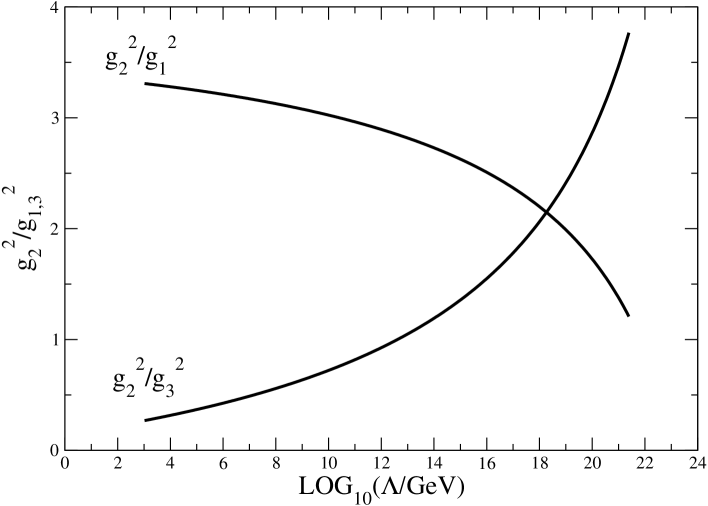
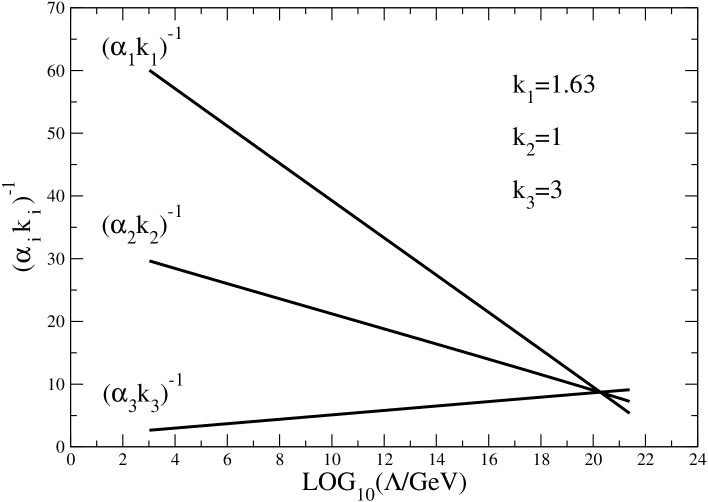
Figure 3: The ratio $g_{2}^{2}/g_{1}^{2}$ (upper curve) and $g_{2}^{2}/g_{3}^{2}$ (lower curve) as functions of the energy scale.

Figure 4: The running of $(\alpha_{1}k_{1})^{-1}$, $(\alpha_{2}k_{2})^{-1}$ and $(\alpha_{3}k_{3})^{-1}$ with $k_{3}=3,k_{2}=1$ and $k_{1}\simeq 1.63$. The unification scale is $10^{20}$ GeV.

As we have seen in the above subsections, the $Z_{4}$ part is anomalous, while the $Z_{6}$ part is anomaly-free. This anomaly is canceled by the GS mechanism if the relation

$$\frac{1\ ({\rm mod}\ 2)}{k_{3}}=\frac{3\ ({\rm mod}\ 2)}{k_{2}}$$ (204)

is satisfied. For example, this is possible if the values of the Kac-Moody levels satisfy $k_{3}=k_{2}$ or $k_{2}=1(3)$ and $k_{3}=3(1)$. Figure 4 displays the ratio of gauge couplings. For the case $k_{3}=k_{2}$ and the case $k_{2}=3$ and $k_{3}=1$, the unification point of the $SU(3)_{C}$ and $SU(2)_{L}$ gauge couplings is far lower than the Planck scale. In the case $k_{2}=1$ and $k_{3}=3$, the $SU(3)_{C}$ and $SU(2)_{L}$ gauge coupling constants can be unified at a scale slightly higher than the Planck scale. In this case, it is also possible to unify $U(1)_{Y}$ at the same point if we assume $k_{1}\simeq 1.63$. Figure 4 plots the running of the gauge couplings in the case $k_{3}=3,k_{2}=1$ and $k_{1}\simeq 1.63$.

8 Summary

In this paper, we have investigated the anomaly of discrete symmetries and their cancellation mechanism. We have seen that the anomalies of discrete symmetries can be defined as the anomalous Jacobian of the path-integral measure, and that if we assume the anomalies are canceled by the GS mechanism, the ordinary conditions of gauge coupling unification can be changed. For the discrete abelian baryon number and lepton number symmetries in the MSSM with the see-saw mechanism, we find that the ordinary unification conditions of the gauge couplings are inconsistent with the GS cancellation conditions, and that the existence of three pairs of $SU(2)_{L}$ Higgs doublets is a possible solution to satisfy the GS cancellation conditions and the unification conditions simultaneously.

We have investigated the cases of several recently proposed supersymmetric models with a non-abelian discrete family symmetry. In the examples considered in this paper, the gauge couplings do not exactly meet at the Planck scale, but we think that the examples suggest the right direction. If we take into account the threshold corrections at $M_{PL}$, for instance, the conditions could be exactly satisfied.

References

-
[1]
E. Ma and G. Rajasekaran, Phys. Rev. D 64 (2001), 113012.
E. Ma, Mod. Phys. Lett. A 17 (2002), 627.
K. S. Babu, E. Ma and J. W. F. Valle, Phys. Lett. B 552 (2003), 207. -
[2]
H. Harari, H. Haut and J. Weyers, Phys. Lett. B 78 (1978), 459.
J. Kubo, A. Mondragón, M. Mondragón and E. Rodríguez-Jáuregui, Prog. Theor. Phys. 109 (2003), 795.
J. Kubo, Phys. Lett. B 578 (2004), 156.
T. Teshima, Phys. Rev. D 73 (2006), 045019. -
[3]
W. Grimus and L. Lavoura, Phys. Lett. B 572 (2003), 189.
W. Grimus, A. S. Joshipura, S. Kaneko, L. Lavoura and M. Tanimoto, J. High Energy Phys. 0407 (2004), 078. - [4] K. S. Babu and J. Kubo, Phys. Rev. D 71 (2005), 056006.
- [5] S. L. Chen and E. Ma, Phys. Lett. B 620 (2005), 151.
- [6] E. Ma, Fizika B 14 (2005), 35.
-
[7]
Y. Kajiyama, J. Kubo and H. Okada, Phys. Rev. D 75 (2007),
033001.
G. Altarelli and F. Feruglio, Nucl. Phys. B 741 (2006), 215.
C. Hagedorn, M. Lindner and R. N. Mohapatra, J. High Energy Phys. 0606 (2006), 042.
C. Hagedorn, M. Lindner and F. Plentinger, Phys. Rev. D 74 (2006), 025007. -
[8]
T. Kobayashi, J. Kubo and H. Terao, Phys. Lett. B 568 (2003),
83.
Y. Kajiyama, E. Itou, J. Kubo, Nucl. Phys. B 743 (2006), 74. -
[9]
M. B. Green and J. H. Schwarz, Phys. Lett. B 149 (1984), 117;
Nucl. Phys. B 255 (1985), 93.
M. B. Green, J. H. Schwarz and P.West, Nucl. Phys. B 254 (1985), 327. -
[10]
E. Witten, Phys. Lett. B 149 (1984), 351.
M. Dine, N. Seiberg and E, Witten, Nucl. Phys. B 289 (1987), 319.
J. Atick, L. Dixion and A. Sen, Nucl. Phys. B 292 (1987), 109.
W. Lerche, B. Nilsson and A. N. Schellekens, Nucl. Phys. B 299 (1988), 91. -
[11]
F. G. Ray, hep-th/9602178.
T. Kobayashi and H. Nakano, Nucl. Phys. B 496 (1997), 103.
P. Ramond, hep-ph/9808488. -
[12]
L. E. Ibáñez and G. G. Ross, Phys. Lett. B 260 (1991),
291; Nucl. Phys. B 368 (1992), 3.
L. E. Ibáñez, Nucl. Phys. B 398 (1993), 301.
T. Bank and M. Dine, Phys. Rev. D 45 (1992), 1424.
H. K. Dreiner, C. Luhn and M. Thormeier, Phys. Rev. D 73 (2006), 075007. -
[13]
K. Kurosawa, N. Maru and T. Yanagida, Phys. Lett. B 512 (2001),
203.
J. Kubo and D. Suematsu, Phys. Rev. D 64 (2001), 115014. - [14] K. S. Babu, I. Gogoladze and K. Wang, Nucl. Phys. B 660 (2003), 322.
-
[15]
H. Dreiner and M. Thormeier, Phys. Rev. D 69 (2004), 053002.
H. Dreiner, H. Murayama and M. Thormeier, Nucl. Phys. B 729 (2005), 278. -
[16]
F. Wegner, J. Math. Phys. 12 (1971), 2259.
L. M. Krauss and F. Wilczek, Phys. Rev. Lett. 62 (1989), 1221. -
[17]
S. Hawking, Phys. Lett. B 195 (1987), 337.
G. V. Lavrelashvili, V. Rubakov and P. Tinyakov, JETP. Lett. 46 (1987), 167.
S. Giddings and A. Strominger, Nucl. Phys. B 306 (1988), 890.
S. Coleman, Nucl. Phys. B 310 (1988), 643. - [18] K. Fujikawa, Phys. Rev. Lett. 42 (1979), 1195; Phys. Rev. D 21 (1980), 2848; Phys. Rev. Lett. 44 (1980), 1733.
- [19] K. Konishi and K. Shizuya, Nuovo. Cim. A 90 (1985), 111.
- [20] See for example E. Ma, hep-ph/0409075.
-
[21]
E. Witten, Nucl. Phys. B 258 (1985), 75.
B. R. Greene, K. H. Kirklin, P. J. Miron and G. G. Ross, Nucl. Phys. B 278 (1986), 667; Phys. Lett. B 180 (1986), 69.
M. Matsuda, T. Matsuoka, H. Mino, D. Suematsu and Y. Yamada, Prog. Theor. Phys. 79 (1987), 174.
T. Kobayashi, H. P. Nilles, F. Plöger, S. Raby and M. Ratz, Nucl, Phys, B 768 (2007), 135. - [22] G. Altarelli, F. Feruglio and Y. Lin, hep-ph/0610165.