DESY 06-239

KEK-TH-1126

KIAS-P06064

SPIN ANALYSIS OF SUPERSYMMETRIC PARTICLES
S.Y. Choi^1,2, K. Hagiwara³, H.-U. Martyn^1,4, K. Mawatari⁵ and P.M. Zerwas^1,3

¹ Deutsches Elektronen-Synchrotron DESY, D-22603 Hamburg, Germany
² Physics Department and RIPC, Chonbuk University, Jeonju 561-756, Korea
³ Theory Division, KEK, Tsukuba, Ibaraki 305-0801, Japan
⁴ I. Physikalisches Institut, RWTH Aachen, Aachen, Germany
⁵ School of Physics, Korea Institute for Advanced Study, Seoul 130-722, Korea

The spin of supersymmetric particles can be determined at $e^{+}e^{-}$ colliders unambiguously. This is demonstrated for a characteristic set of non-colored supersymmetric particles – smuons, selectrons, and charginos/neutralinos. The analysis is based on the threshold behavior of the excitation curves for pair production in $e^{+}e^{-}$ collisions, the angular distribution in the production process and decay angular distributions. In the first step we present the observables in the helicity formalism for the supersymmetric particles. Subsequently we confront the results with corresponding analyses of Kaluza-Klein particles in theories of universal extra space dimensions which behave distinctly different from supersymmetric theories. It is shown in the third step that a set of observables can be designed which signal the spin of supersymmetric particles unambiguously without any model assumptions. Finally in the fourth step it is demonstrated that the determination of the spin of supersymmetric particles can be performed experimentally in practice at an $e^{+}e^{-}$ collider.

1 INTRODUCTION

The spin is one of the characteristics of all particles and it must be determined experimentally for any new species. Compelling arguments have been forwarded which suggest the supersymmetric extension of the Standard Model [1, 2]. In supersymmetric theories (SUSY) spin-1 gauge and spin-0 Higgs bosons are paired with spin-1/2 fermions, gauginos and higgsinos, which mix, in the non-colored sector, to form charginos and neutralinos. Analogously spin-1/2 leptons and quarks are paired with spin-0 scalar sleptons and squarks. This opens a wide area of necessary efforts to determine the nature of the new particles experimentally.

Measuring the masses of the particles is not sufficient to unravel the nature of the particles and of the underlying theory. This point has been widely discussed by comparing supersymmetric theories with theories of universal extra space dimensions (UED) [3, 4] in which the counterparts of the supersymmetric partners are Kaluza-Klein (KK) excitations of the standard particles. When supersymmetric squarks are produced [5] at LHC, they may cascade down [6] to standard particles in the chain $\tilde{q}\to q\tilde{\chi}^{0}_{2}\to q\bar{\ell}\tilde{\ell}\to q\bar{\ell}\ell\tilde{\chi}^{0}_{1}$, which generates the observable final state $q\bar{\ell}\ell$. However, an analogous cascade can be realized in theories of universal extra space dimensions, starting from a KK excitation $q_{1}$ of a quark, $q_{1}\to qZ_{1}\to q\bar{\ell}\ell_{1}\to q\bar{\ell}\ell\gamma_{1}$ [7]. The origin of the observed chain particles, supersymmetry or extra space dimensions, can clearly be unraveled by measuring the spins of the intermediate cascade particles.

Spin measurements of supersymmetric particles are difficult at LHC [7, 8, 9]. While the invariant mass distributions of the particles in decay cascades are characteristic for the spins of the intermediate particles involved, detector effects strongly reduce the signal in practice.

In contrast, several techniques can be exploited to determine unambiguously the spin of particles produced pairwise in $e^{+}e^{-}$ collisions. These techniques have first been worked out theoretically for Higgs bosons, studied in the Higgs-strahlung process [10]; subsequent experimental simulations have proven these techniques to work in practice [11]. To conform with its scalar character, the polar angle distribution in smuon pair production has been investigated directly by reconstruction in Ref. [12] and reflected in their decay products in Ref. [13] at TeV and multi-TeV $e^{+}e^{-}$ colliders, respectively.

A sequence of techniques, increasing in complexity, can be applied to determine the spin of particles in pair production

$$e^{+}e^{-}\ \ \to\ \ \tilde{\mu}^{+}\tilde{\mu}^{-},\,\tilde{e}^{+}\tilde{e}^{-}\;\;{\rm and}\;\;\,\tilde{\chi}^{+}\tilde{\chi}^{-},\,\tilde{\chi}^{0}\tilde{\chi}^{0}$$ (1.1)

of sleptons, charginos and neutralinos in $e^{+}e^{-}$ collisions:

• (a) rise of the excitation curve near the threshold;
  

• (b) angular distribution in the production process;
  

• (c) angular distribution in decays of the polarized particles,

eventually supplemented by

• (d) angular correlations between decay products of two particles.
  

While the second step (b) is already sufficient in the slepton sector, only the final state analysis is sufficient in general, including charginos/neutralinos, to determine the spin unambiguously. On the experimental side we follow the standard path. It will be shown in detailed simulations that the theoretically predicted distributions in supersymmetric theories can be reconstructed after including initial and final state QED radiation, beamstrahlung and detector effects. Within the extended theoretical frame it is then proven that the assignment of the spin is unambiguous indeed.

The report is organized as follows. In the subsequent Sections 2 to 4 we set up the theoretical basis for spin measurements of smuons, selectrons, and charginos/neutralinos. The technical frame we have chosen is the helicity formalism. We analyze which observables must be measured to determine the spin unambiguously. Moreover, simulations will assure us that the analyses of supersymmetric theories in $e^{+}e^{-}$ collisions can be performed experimentally. In the last Section 5 we briefly summarize the results. General formulae for the production cross sections of supersymmetric particles in collisions of polarized electrons and positrons are presented in an Appendix.

2 SPIN OF SMUONS

2.1 Smuon Production in $e^{+}e^{-}$ Collisions

Smuons are the prototype for scalar particle pair production in $e^{+}e^{-}$ collisions [14, 15] mediated by the $s$-channel exchange of $\gamma$ and $Z$ boson. Different lepton numbers prevent the flow of particles from the initial to the final state. For the sake of [experimental] simplicity we will restrict ourselves to the analysis of R-type smuons,

$$e^{+}e^{-}\ \ \rightarrow\ \ \tilde{\mu}^{+}_{R}\,\tilde{\mu}^{-}_{R}$$ (2.1)

as these particles almost exclusively decay through the 2-particle channel $\tilde{\mu}^{\pm}_{R}\to\mu^{\pm}\tilde{\chi}^{0}_{1}$ with only one escaping invisible particle. The process is described by diagram (a) in Fig. 1.

Figure 1: (a) $s$-channel $\gamma$ and $Z$ exchange diagrams contributing to the production of all slepton pairs in $e^{+}e^{-}$ annihilation; and (b) $t$-channel neutralino exchange diagram contributing only to the production of selectron pairs in $e^{+}e^{-}$ collisions.

The amplitude describing this production process can be expressed in terms of the generalized electron charges

$$Q_{L}=1+\left(s^{2}_{W}-1/2\right)c^{-2}_{W}D_{Z}(s)$$ (2.2)

$$Q_{R}=1+t^{2}_{W}D_{Z}(s)$$ (2.3)

with $s^{2}_{W}=\sin^{2}\theta_{W}$ etc, $\theta_{W}$ being the electroweak mixing angle, and the normalized $Z$ propagator $D_{Z}(s)=s/[s-m^{2}_{Z}+im_{Z}\Gamma_{Z}]$, $s$ denoting the squared center-of-mass energy [$D_{Z}$ is approximately real in the high energy limit $s\gg m^{2}_{Z}$]. The indices $L$ and $R$ in Eqs. (2.2) and (2.3) refer to left- and right-handedly polarized electrons [and oppositely polarized positrons], respectively.

The total cross section and the distribution in the polar angle $\theta$ between the $\tilde{\mu}^{\pm}$ flight direction and the $e^{+}e^{-}$ beam axis can be written in the form

$$\sigma\left[e^{+}e^{-}\to\tilde{\mu}^{+}_{R}\tilde{\mu}^{-}_{R}\right] = \frac{\pi\alpha^{2}}{6s}\beta^{3}\left[Q^{2}_{L}+Q^{2}_{R}\right]$$ (2.4)

$$\frac{1}{\sigma}\frac{d\sigma}{d\cos\theta}\left[e^{+}e^{-}\to\tilde{\mu}^{+}_{R}\tilde{\mu}^{-}_{R}\right] = \frac{3}{4}\sin^{2}\theta$$ (2.5)

The coefficient $\beta^{3}$, with $\beta=(1-4m^{2}_{\tilde{\mu}_{R}}/s)^{1/2}$ denoting the velocity of the smuons, is the product of the phase space suppression factor $\beta$, and the square of the $P$-wave suppression $\sim\beta$ near the threshold. The scalar smuon pair is produced in a $P$-wave to balance the spin 1 of the intermediate vector boson. Angular momentum conservation leads also to the $\sin^{2}\theta$ dependence of the differential cross section as forward production of spinless particles is forbidden.

For asymptotic energies the cross section

$$\sigma\ \ \to\ \ \frac{5\pi\alpha^{2}}{24c_{W}^{4}}\,\frac{1}{s}\quad\mbox{for}\quad s\ \ \rightarrow\ \ \infty$$ (2.6)

follows the appropriate scaling law.

The production of spin-0 particles in $e^{+}e^{-}$ annihilation is thus described by two characteristics:

$$\#1\quad\mbox{threshold excitation}\quad\sim\ \ \beta^{3}$$ (2.7)

$$\#2\quad\mbox{angular distribution}\quad\sim\ \ \sin^{2}\theta$$ (2.8)

The threshold excitation for smuons and the angular distribution are illustrated in Fig. 2(a) and (b), respectively. The $\tilde{\mu}_{R}$ mass is chosen $m_{\tilde{\mu}_{R}}=300$ GeV. In the following subsections it will be proven that the angular distribution is characteristic indeed for spinless particles and that it can be measured with great accuracy in $e^{+}e^{-}$ collisions.

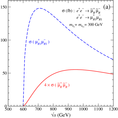
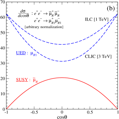
Figure 2: (a) The threshold excitation for smuons; and (b) the angular distribution in $e^{+}e^{-}\to\tilde{\mu}^{+}_{R}\tilde{\mu}^{-}_{R}$ [arbitrary normalization]. The predictions for smuons are compared with the corresponding observables for the first KK excitation $\mu_{R1}^{\pm}$ in $e^{+}e^{-}\to{\mu}^{+}_{R1}{\mu}^{-}_{R1}$.

2.2 KK Excited States $\mu^{\pm}_{1}$ in UED

The minimal UED version with one universal extra space dimension, which is compactified on the orbifold $S_{1}/Z_{2}$, generates a tower of spin-1/2 KK states over each L-type and R-type fermion in the Standard Model (SM) without generating additional zero modes [3]. Focussing on the R-type states in analogy to the previous subsection, the process for the production of a pair of the first muonic KK excitation,

$$e^{+}e^{-}\ \ \rightarrow\ \ \mu^{+}_{R1}\,\mu^{-}_{R1}$$ (2.9)

is described by the same diagram Fig. 1(a). $\mu^{\pm}_{R1}$ is a massive Dirac fermion carrying the electroweak charges of $\mu^{\pm}_{R}$ but coupling only through vector currents to the electroweak gauge bosons $\gamma$ and $Z$. Thus the generalized charges are identical with Eqs. (2.3) and (2.2). It decays into the $\mu^{\pm}_{R}\gamma_{1}$ channel where $\gamma_{1}$ is the lightest and stable excited gauge boson generally identified with the U(1) boson.

The total cross section and the angular distribution are markedly different from the supersymmetric case:

$$\sigma[e^{+}e^{-}\to\mu^{+}_{R1}\mu^{-}_{R1}] = \frac{2\pi\alpha^{2}}{3s}\,\beta\,\frac{(3-\beta^{2})}{2}\left[Q^{2}_{L}+Q^{2}_{R}\right]$$ (2.10)

$$\frac{1}{\sigma}\frac{d\sigma}{d\cos\theta}\,[e^{+}e^{-}\to\mu^{+}_{R1}\mu^{-}_{R1}] = \ \ \frac{3}{8}\frac{2}{(3-\beta^{2})}\left[1+\cos^{2}\theta+(1-\beta^{2})\sin^{2}\theta\right]$$ (2.11)

[Because of the vector character of the electroweak $\mu_{R1}$ currents the distribution is symmetric in forward and backward direction.] The $\mu_{R1}$ pair is produced in an $S$-wave with non-vanishing amplitude at the origin. The onset of the excitation curve is therefore suppressed only by the phase space factor $\sim\beta$. The angular distribution is familiar from QED, being isotropic at threshold and evolving to the transverse-polarization term $(1+\cos^{2}\theta)$ asymptotically.

For high energies the total cross section

$$\sigma\ \ \to\ \ \frac{20\pi\alpha^{2}}{24c_{W}^{4}}\,\frac{1}{s}\quad\mbox{for}\quad s\ \ \rightarrow\ \ \infty$$ (2.12)

scales in the same way as the $\tilde{\mu}^{+}\tilde{\mu}^{-}$ cross section but with a coefficient 4 times as large, as familiar from QED processes.

Choosing for illustration a $\mu^{\pm}_{R1}$ mass of 300 GeV, a value at the lower limit of the experimentally allowed range [3], the onset of the cross section and the angular distribution are displayed in Fig. 2(a) and (b). The center-of-mass energy is set to $\sqrt{s}=1$ TeV for ILC [14] and 3 TeV for CLIC [15] in the second figure. Both characteristics are markedly different from supersymmetric theories; see also Ref. [13]. In contrast to scalar smuons the onset of the excitation is vertical, proportional to the velocity $\beta\sim[s-4m^{2}_{\mu_{R1}}]^{1/2}$ as familiar for spin-1/2 particles. Also the angular distributions for scalar smuons and fermionic KK muon states are distinctly different.

Already from the totally inclusive measurement of the production cross section no more confusion can arise between supersymmetric theories and theories of universal extra space dimensions.

2.3 General Analysis

Though the difference between the characteristics in the production of supersymmetric scalar particles and KK excited fermions can be exploited to rule out the false theory experimentally, we should explore nevertheless whether the conditions (2.7) and/or (2.8) are not only necessary but also sufficient to single out the scalar solution.

The general analysis is most transparent if performed in the helicity formalism. In the process

$$e^{+}e^{-}\ \ \to\ \ F^{J}_{\lambda_{1}}\bar{F}^{J}_{\lambda_{2}}$$ (2.13)

for pointlike particles $F^{J}$ and $\bar{F}^{J}$ with spin $J$ and helicities $\lambda_{1}$ and $\lambda_{2}$ [either half-integer or integer], and mediated by $s$-channel $\gamma$ and $Z$ exchange, the helicities of the electron and positron in the initial state are coupled to a vector with spin $m=\pm 1$ along the beam axis. The right-hand side of the diagram in Fig. 1(a) may then be interpreted as the decay of a virtual vector boson with polarization $m=\pm 1$ to the $F^{J}\bar{F}^{J}$ pair. If the flight axis of the $F^{J}$ particles includes the angle $\theta$ with the vector boson polarization axis [identical with the $e^{\pm}$ beam axis], the decay amplitude may be expressed in term of the helicity amplitude ${\cal T}_{\lambda_{1}\lambda_{2}}$,

$$\langle F^{J}_{\lambda_{1}}\bar{F}^{J}_{\lambda_{2}};\theta|V_{m}\rangle=\sqrt{2s}\,g_{V}\,d^{1}_{m,\lambda^{\prime}}(\theta)\,{\cal T}_{\lambda_{1}\lambda_{2}}\quad\mbox{with}\quad\lambda^{\prime}=\lambda_{1}-\lambda_{2}$$ (2.14)

The angular dependence is in total encoded in the Wigner $d$ function while the reduced helicity amplitudes ${\cal T}_{\lambda_{1}\lambda_{2}}$ are independent of $m$. The value of $\lambda^{\prime}$ is restricted to $\lambda^{\prime}=0$ and $\pm 1$. The totally inclusive cross section can be expressed in the form

$$\sigma=\frac{\pi\alpha^{2}}{3s}\,\beta\,\left(Q^{2}_{L}+Q^{2}_{R}\right)\left[\sum_{\lambda}\left(|{\cal T}_{\lambda,\lambda-1}|^{2}+|{\cal T}_{\lambda,\lambda+1}|^{2}\right)+\sum_{\lambda}|{\cal T}_{\lambda\lambda}|^{2}\right]$$ (2.15)

and the forward-backward symmetric part of the differential cross section analogously as

$$\frac{d\sigma^{\prime}}{d\cos\theta}=\frac{\pi\alpha^{2}}{4s}\beta\left(Q^{2}_{L}+Q^{2}_{R}\right)\left[\frac{1+\cos^{2}\theta}{2}\sum_{\lambda}\left(|{\cal T}_{\lambda,\lambda-1}|^{2}+|{\cal T}_{\lambda,\lambda+1}|^{2}\right)+\sin^{2}\theta\sum_{\lambda}|{\cal T}_{\lambda\lambda}|^{2}\right]$$ (2.16)

summed over the helicities of the outgoing $F^{J}$ and $\bar{F}^{J}$ particles. To evaluate these expressions, the two cases in which $F^{J}$ is either fermionic or bosonic must be distinguished.

(a) Fermionic spectrum $F[J=1/2,3/2,\ldots]$:
For pointlike theories in which the fermions carry electric and weak monopole charges the associated vector current includes the basic component [19]

$$j^{0}_{\mu}=\bar{\psi}_{\alpha_{1}\cdots\alpha_{n}}\gamma_{\mu}\psi^{\alpha_{1}\cdots\alpha_{n}}$$ (2.17)

built by the $J=n+1/2$ spinor-tensor wave-function $\psi^{\alpha_{1},\ldots,\alpha_{n}}$ [20]. In analogy to the Dirac spin 1/2 case, the current (2.17) can be decomposed, cf. Refs. [19, 21], into an electric current $j^{e}_{\mu}$ and a magnetic current $j^{m}_{\mu}$ as $j_{\mu}=j^{e}_{\mu}+j^{m}_{\mu}$ with

$$j^{e}_{\mu}=\frac{1}{2m}\bar{\psi}_{\alpha_{1},\ldots,\alpha_{n}}\,\,i\,\overleftrightarrow{\partial_{\mu}}\,\,\psi^{\alpha_{1},\ldots,\alpha_{n}}$$ (2.18)

$$j^{m}_{\mu}=\frac{1}{2m}\partial^{\nu}\left(\bar{\psi}_{\alpha_{1},\ldots,\alpha_{n}}\,\,\sigma_{\mu\nu}\,\,\psi^{\alpha_{1},\ldots,\alpha_{n}}\right)$$ (2.19)

reducing to electric monopole and magnetic dipole currents in the non-relativistic limit.

Both the electric current $j^{e}_{\mu}$ and the magnetic current $j^{m}_{\mu}$ give rise to diagonal reduced helicity amplitudes through spin-0/$D$-wave and spin-1/$S$-wave interactions, respectively; apart from overall coefficients,

$${\cal T}^{e}_{\lambda\lambda}\,=\,\phantom{-}\frac{\gamma\beta^{2}}{\sqrt{2}}\left[\frac{(J+\lambda)}{2J}\,Q^{J-1/2}_{\lambda-1/2}(\gamma)-\frac{(J-\lambda)}{2J}\,Q^{J-1/2}_{\lambda+1/2}(\gamma)\right]$$ (2.20)

$${\cal T}^{m}_{\lambda\lambda}\,=\,\,-\frac{\gamma}{\sqrt{2}}\left[\frac{(J+\lambda)}{2J}\,Q^{J-1/2}_{\lambda-1/2}(\gamma)-\frac{(J-\lambda)}{2J}\,Q^{J-1/2}_{\lambda+1/2}(\gamma)\right]$$ (2.21)

Only the magnetic dipole current $j^{m}_{\mu}$ generates non-diagonal reduced helicity amplitudes,

$${\cal T}^{m}_{\lambda,\lambda\pm 1}\,=\,\mp\frac{\sqrt{(J\mp\lambda)(J\pm\lambda+1)}}{2J}\,\,Q^{J-1/2}_{\lambda\pm 1/2}(\gamma)$$ (2.22)

Here, $\gamma=\sqrt{s}/2m$ is the Lorentz boost factor of the final-state particle and the energy-dependent functions $Q^{N}_{n}(\gamma)$ ($|n|\leq N$ for integral $N$ and $n$) are defined as

$$Q^{N}_{n}(\gamma) = \frac{2^{N}(N+n)!\,(N-n)!}{(2N)!}\,\sum_{\lambda_{1}=\pm 1,0}\cdots\sum_{\lambda_{N}=\pm 1,0}\,\delta_{n,\lambda_{1}+\cdots+\lambda_{N}}\,\prod_{i=1}^{N}\frac{(2\gamma^{2}\delta_{\lambda_{i}0}-1)}{(1+\lambda_{i})!\,(1-\lambda_{i})!}$$ (2.23)

$$Q^{\,0}_{0}(\gamma) = 1\quad\mbox{and}\quad Q^{N}_{n}(\gamma)\,=\,0\quad\mbox{for}\quad|n|>N\geq 0$$ (2.24)

We note that the non-diagonal reduced helicity amplitudes ${\cal T}_{\lambda,\lambda\pm 1}={\cal T}^{m}_{\lambda,\lambda\pm 1}$ are non-vanishing for any energy. As a result, the term $\sum_{\lambda}\left(|{\cal T}_{\lambda,\lambda-1}|^{2}+|{\cal T}_{\lambda,\lambda+1}|^{2}\right)$ never vanishes, leading to a cross section that rises $\sim\beta$ at the threshold and contributing with a term $\sim(1+\cos^{2}\theta)$ to the angular distribution. Both elements differ clearly from the production of scalar particles. We therefore conclude that scalar spin-0 particles in supersymmetric theories carrying muon-type charges can never be confused by fermionic charged particles.

(b) Bosonic spectrum $F[J=1,2,\ldots]$:
Restricting ourselves to CP-invariant theories, the electric and weak monopole charge term of any integer spin $J$ tensor-field $\varphi^{\alpha_{1}..\alpha_{J}}$ is accounted for by the current element

$$j^{e}_{\mu}\,=\,i\,\,\varphi^{*}_{\alpha_{1}\cdots\alpha_{J}}\,\,\overleftrightarrow{\partial_{\mu}}\,\,\varphi^{\alpha_{1}\cdots\alpha_{J}}$$ (2.25)

It leads to $P$-wave production of the boson pair with the reduced helicity amplitude

$${\cal T}^{e}_{\lambda\lambda}\,=\,-\frac{\beta}{\sqrt{2}}\,Q^{J}_{\lambda}(\gamma)$$ (2.26)

Since the wave-function vanishes at the origin, the total production cross section rises $\sim\beta^{3}$ at the threshold. Thus, opposite to wide-spread belief, the onset of the excitation curve near threshold does not discriminate the spin 0 particle from higher integer spin $J=1,2,\ldots$ particles.

However, coupling the electroweak vector fields to the spin $J$ fields in a consistent way [19], a non–vanishing magnetic dipole moment is generated for all particles with spin $>0$. The non–zero magnetic current, which is proportional to

$$j^{m}_{\mu}=-i\,\partial^{\nu}(\varphi_{[\mu}^{*\alpha_{2}\ldots\alpha_{J}}\,\varphi_{\nu]\alpha_{2}\ldots\alpha_{J}})$$ (2.27)

gives rise to non-vanishing off-diagonal helicity amplitudes which can be written, apart from an overall coefficient, as

$${\cal T}^{m}_{\lambda,\lambda\pm 1}\,=\,-\gamma\beta\,\frac{\sqrt{(J\mp\lambda)(J\pm\lambda+1)}}{2J(2J-1)}\,\left[(J\pm\lambda)\,Q^{J-1}_{\lambda}(\gamma)+(J\mp\lambda-1)\,Q^{J-1}_{\lambda\pm 1}(\gamma)\right]$$ (2.28)

The $P$-wave behavior near the threshold is reflected in the coefficient $\beta$. The non-vanishing helicity amplitude ${\cal T}_{\lambda,\lambda\pm 1}={\cal T}^{m}_{\lambda,\lambda\pm 1}$ for $J>0$ is in apparent contrast to spin-0 scalars for which these amplitudes must vanish. Thus opposite to scalar production, higher spin $J=1,2,..$ production will generate an additional term $\sim(1+\cos^{2}\theta)$ in the angular distribution, non-vanishing in the forward and backward direction. Thus the analysis of the angular distributions signals the zero-spin of the smuons unambiguously.

Complementary to this theory-based argument on production properties, i.e. the onset of the excitation curve and the angular distribution, decay characteristics can also be exploited to supplement the analysis. The presence of the off-diagonal helicity amplitudes, Eq. (2.22) for fermions and Eq. (2.28) for bosons, implies that the final state particles $F^{J}$ and $\bar{F}^{J}$ should be polarized when electron and/or positron beams are polarized. In addition, the relation $\lambda_{1}-\lambda_{2}=\pm 1$ for the non-vanishing off-diagonal helicities of the $F^{J}_{\lambda_{1}}\bar{F}^{J}_{\lambda_{2}}$ pair produced via $\gamma,Z$ exchange should lead to interesting polarization correlations which can be observed through the correlated decays of $F^{J}_{\lambda_{1}}$ and $\bar{F}^{J}_{\lambda_{2}}$. In this case, the polar-angle distribution of the decay particles in the $F^{J}$ rest frame is described by the Wigner $d$ function,

$$\mathcal{D}\left[F^{J}_{\lambda}\rightarrow a_{\sigma_{1}}b_{\sigma_{2}}\right]\,\,\sim\,\,d^{J}_{\lambda\sigma}(\theta^{*})\quad\mbox{with}\quad\sigma=\sigma_{1}-\sigma_{2}$$ (2.29)

where $\theta^{*}$ denotes the polar angle between the $F^{J}$ flight direction and the $ab$ axis in the $F^{J}$ rest frame. This configuration is realized in the dominant $\mu\tilde{\chi}^{0}_{1}$ decay channel of $\tilde{\mu}_{R}$. For scalar smuons $d^{0}_{00}(\theta^{*})$ does not depend on $\theta^{*}$. For $J>0$, however, even if the final-state polarizations $\sigma_{1},\sigma_{2}$ are summed over, the angular distribution is always non-trivial when the sum of two final-state daughter spins, $j_{a}$ and $j_{b}$, is less than the spin $J$ of the parent. In the opposite case, $j_{a}+j_{b}\geq J$, parity-violating decays in general guarantee non-trivial angular dependence; only in parity-preserving cases the decay distribution might be independent of the $F^{J}$ polarization. However, if the final-state polarizations $\sigma_{1},\sigma_{2}$ are measured, the $\theta^{*}$ dependence of $d^{J}_{\lambda\sigma}(\theta^{*})$ for $J>0$ is always non-trivial, whatever values are taken for $|\lambda|$ and $|\sigma|\leq J$. After squaring the decay amplitude $\mathcal{D}$, the spin $J$ can be determined by projecting out the maximum spin index $2J$ from the decay angular distributions.

Therefore the analysis of the smuon decay distributions provides us with an alternative model-independent method for the determination of the zero smuon spin.

2.4 Reconstructing the Event Axis

(a) ${\tilde{\mu}_{R}}^{+}{\tilde{\mu}_{R}}^{-}$ in supersymmetry:
The measurement of the cross section for smuon pair production $\tilde{\mu}^{+}_{R}\tilde{\mu}^{-}_{R}$ can be carried out by identifying acoplanar $\mu^{+}\mu^{-}$ pairs [with respect to the $e^{\pm}$ beam axis] accompanied by large missing energy:

$$e^{+}e^{-}\ \ \rightarrow\ \ \tilde{\mu}^{+}_{R}\,\tilde{\mu}^{-}_{R}\ \ \rightarrow\ \ (\mu^{+}\tilde{\chi}^{0}_{1})\;(\mu^{-}\tilde{\chi}^{0}_{1})\ \ \to\ \ \mu^{+}\mu^{-}\not\!\!{E}\$$ (2.30)

The analysis is model-independent and it provides unambiguously the onset of the excitation curve $\sim\beta^{3}$ near threshold.

The construction of the production angle $\theta$ is illustrated for the event topology in Fig. 3. For very high energy $\sqrt{s}\gg m_{\tilde{\mu}_{R}}$ the flight direction of the daughter particles $\mu^{\pm}$’s can be approximated by the flight direction of the parent particle [13] and the dilution due to the decay kinematics is small. However, at medium ILC energies the dilution increases, and the reconstruction of the $\tilde{\mu}^{\pm}_{R}$ flight direction provides more accurate results on the angular distribution of the smuon pairs [12]. If all particle masses are known, the magnitude of the particle momenta is calculable and the relative orientation of the momentum vectors of $\mu^{\pm}$ and ${\tilde{\mu}_{R}}^{\pm}$ is fixed by the two-body decay kinematics. The opening angles $\alpha_{\pm}$ between the visible $\mu^{\pm}$ tracks and the parent $\tilde{\mu}^{\pm}_{R}$ particles can be determined from the relation

$$m^{2}_{\mu^{\pm}_{R}}-m^{2}_{\tilde{\chi}^{0}_{1}}=\sqrt{s}E_{\mu^{\pm}}(1-\beta_{\tilde{\mu}^{\pm}_{R}}\cos\alpha_{\pm})$$ (2.31)

The angles $\alpha_{\pm}$ define two cones about the $\mu^{+}$ and $\mu^{-}$ axes which intersect in two lines – the true $\tilde{\mu}^{\pm}_{R}$ flight direction and a false direction. True and false solutions are mirrored on the plane spanned by the $\mu^{+}$ and $\mu^{-}$ flight directions. Thus the flight direction can be reconstructed up to a 2-fold ambiguity.

Figure 3: Event topology of the reaction $e^{+}e^{-}\to{\tilde{\mu}_{R}}^{+}{\tilde{\mu}_{R}}^{-}\to\mu^{+}{\tilde{\chi}^{0}}_{1}\,\mu^{-}{\tilde{\chi}^{0}}_{1}$

The characteristics of the angle $\theta_{ft}$ between the false and the true axis can easily be illustrated. If the decay planes of $\tilde{\mu}^{+}_{R}$ and $\tilde{\mu}^{-}_{R}$ coincide, the production axis is located in the common plane and the false axis coincides with the true axis. Rotating one of the two planes away from the other by an azimuthal angle $\phi$, the angle $\theta_{ft}$ between the false and the true axis is related to $\phi$ and to the boosts $\gamma_{\pm}=\gamma(\cos\alpha^{*}_{\pm}+\beta)/\sin\alpha^{*}_{\pm}$ with $\alpha^{*}_{\pm}$ being the $\tilde{\mu}^{\pm}_{R}\to\mu^{\pm}$ decay angle in the $\tilde{\mu}^{\pm}_{R}$ rest frame with respect to the flight direction in the laboratory frame:

$$\cos\theta_{ft}=1-\frac{2\sin^{2}\phi}{\gamma^{2}_{+}+\gamma^{2}_{-}+2\gamma_{+}\gamma_{-}\cos\phi+\sin^{2}\phi}$$ (2.32)

For high energies the maximum opening angle reduces effectively to $\theta_{ft}\lesssim{\rm min}(1/|\gamma_{+}|,1/|\gamma_{-}|)=O(1/\gamma)$ and approaches zero asymptotically when the two axes coincide. Quite generally, as a result of the Jacobian root singularity in the relation between $\cos\theta_{ft}$ and $\phi$, the false solutions tend to accumulate slightly near the true axis for all energies. In total, the angular distribution of the false axis with respect to the true axis is given by

$$\frac{dN}{d\cos\theta_{ft}}\,=\,\frac{\sqrt{2}}{\sqrt{1-\cos\theta_{ft}}}\cdot\frac{F\left[\beta\cos(\theta_{ft}/2)\right]}{\gamma^{4}\beta^{4}\left(1-\cos\theta_{ft}+2/\gamma^{2}\beta^{2}\right)^{2}\,}$$ (2.33)

with $F[0]=1$ at threshold and $F[\beta]\sim\gamma$ for $\beta\to 1$. The decrease of the coefficient $\sim 1/\gamma^{4}$ is compensated by the effective narrowing of $\theta_{ft}$ in the denominator and by the increase of the function $F$ for rising energy. Thus, the false axis is trailed by the true axis, mildly at low energies and tightly at high energies. Though the distribution of the false axis is flattened at low to medium energies compared with the original distribution of the true axis, the characteristic features are reflected qualitatively, nevertheless, cf. Fig. 4. For our theoretical investigation throughout the paper, the R-type slepton mass $m_{\ell_{R}}=300$ GeV and sneutrino mass $m_{\tilde{\nu}}=365$ GeV are used and the chargino/neutralino mass spectra and the mixing elements are derived from the SUSY Lagrangian parameters $M_{2}=$ 300 GeV, $M_{1}=$ 150 GeV, $\mu=$ 500 GeV and $\tan\beta=10$. This parameter set includes the lighter chargino mass $m_{\tilde{\chi}^{\pm}_{1}}=286$ GeV and to the two lowest neutralino masses $m_{\tilde{\chi}^{0}_{1/2}}=148/286$ GeV.

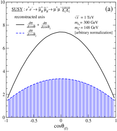
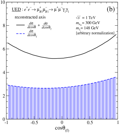
Figure 4: (a) The angular distribution of the false reconstructed axis (blue shaded area) and of the observable sum of true and false axes for smuon pair production in SUSY (black); (b) The same for $\mu^{+}_{R1}\mu^{-}_{R1}$ pair production in UED. [The distribution of the false axis is slightly forward-backward asymmetric due to the parity violating $\mu^{\pm}_{R1}\to\mu^{\pm}\gamma_{1}$ decay.]

Experimentally, the absolute orientation in space is operationally obtained by rotating the two ${\tilde{\mu}_{R}}^{\pm}$ vectors around the $\mu^{\pm}$ axes against each other until they are aligned back-to-back in opposite directions. The flattened false-axis distribution can be subtracted on the basis of Monte Carlo simulations. For a fraction of events the production angle cannot be reconstructed, which in most cases is due to large initial state radiation and/or beamstrahlung reducing the nominal center of mass energy considerably. In addition losses occur due to measurement errors of the final particles. It is also important to note that background events, if they can be reconstructed at all under the wrong (mass) hypothesis, usually produce flat angular distributions and can thus be easily subtracted.

(b) $\mu^{+}_{R1}\mu^{-}_{R1}$ in UED:
As proven in the previous subsection, the experimental observation of the $\sin^{2}\theta$ law determines the spin-0 character of new particles carrying non-electron fermion numbers, i.e. smuons, squarks, etc, unambiguously. This general conclusion can be illuminated by analyzing the spin-1/2 angular distribution of the UED KK excitation $\mu^{\pm}_{R1}$. The [non-normalized] angular distribution of $\mu^{+}_{R1}\mu^{-}_{R1}$ pairs in $e^{+}e^{-}$ collisions is described in Eq. (2.11): $N(\theta)=1+\cos^{2}\theta\,+\,(1-\beta^{2})\,\sin^{2}\theta$. The decay $\mu^{\pm}_{R1}\to\mu^{\pm}\gamma_{1}$ in the $\mu^{\pm}_{1}$ rest frame is governed by the right-handed coupling between the two leptons so that $\mu^{-}$, including the angle $\theta_{1}$ with the $\mu^{-}_{R1}$ polarization vector, is preferentially emitted in the direction parallel to the $\mu_{R1}^{-}$ polarization vector, $D(\theta_{1})=(1+\kappa_{R1}\cos\theta_{1})^{2}$ with $\kappa_{R1}=(m^{2}_{\mu_{R1}}-2m^{2}_{\gamma 1})/(m^{2}_{\mu_{R1}}+2m^{2}_{\gamma 1})\sim 1/3$. The opposite rule applies to $\mu_{R1}^{+}$ decays.

Properly including the correlations among the two decay pairs, the predictions for the distributions of the true production axis, $N(\theta)$, and the false axis, $N_{f}(\theta)$, are displayed in Fig. 4(b). After subtracting the distribution of the false axis from the sum, the distribution of the true axis is markedly different from the distribution of the smuon polar production angle in Fig. 4(a). In particular, the production of spin-1/2 KK muons populates the forward and backward directions in contrast to spin-0 smuons.

This method can be applied quite generally in $e^{+}e^{-}$ annihilation through $\gamma$ and $Z$ exchange for any given theory. For the set $\{c_{1},c_{2}\}$ of coefficients in the true angular distribution

$$N(\theta)\ \ \sim\ \ c_{1}\,[1+\cos^{2}\theta]+c_{2}\,\sin^{2}\theta$$ (2.34)

the false distribution $N_{f}(\theta)$ can be generated unambiguously. Comparing the sum of the distributions of the experimentally reconstructed true and false events with $N+N_{f}$, the ratio of the two coefficients $c_{2}/c_{1}$ can be fitted by using template methods. The fit will only be acceptable if at the same time the helicity structure of the decay vertex is chosen correctly.

2.5 Experimental Analysis

(a) Sparticle spectrum: In order to perform a realistic simulation of signal and background processes a sparticle spectrum is calculated using the program Isajet 7.74 [23]. The SUSY point described above can well be embedded in a mSUGRA scenario with the parameters $m_{0}=265\;\mathrm{GeV},M_{1/2}=375\;\mathrm{GeV},\tan\beta=10,A_{0}=0,$ and ${\rm sign}\,\mu=+1$, corresponding to the Lagrangian parameters $M_{1}=156\;\mathrm{GeV},M_{2}=291\;\mathrm{GeV},\mu=488\;\mathrm{GeV}$. The masses of the R/L-type smuons/selectrons, electron sneutrino, lighter chargino and two lightest neutralinos accessible at a 1 TeV ILC and relevant for the present experimental study are listed in Table 1.

Table 1: Spectrum of sleptons, charginos and neutralinos in the SUSY scenario ($M_{1}=156\;\mathrm{GeV},M_{2}=291\;\mathrm{GeV},\mu=488\;\mathrm{GeV}$).

${\tilde{\ell}}$	m [GeV]		${\tilde{\chi}}$	m [GeV]
${\tilde{e}_{R}}/{\tilde{\mu}_{R}}$	302		${\tilde{\chi}}_{1}^{\pm}$	285
${\tilde{e}_{L}}/{\tilde{\mu}_{L}}$	369		${\tilde{\chi}}_{1}^{\pm}$	510
${\tilde{\nu}}_{e}/{\tilde{\nu}}_{\mu}$	359		${\tilde{\chi}^{0}}_{1}$	152
$\tilde{\tau}_{1}$	297		${\tilde{\chi}^{0}}_{2}$	284
$\tilde{\tau}_{2}$	369		${\tilde{\chi}^{0}}_{3}$	493
$\tilde{\nu}_{\tau}$	357		${\tilde{\chi}^{0}}_{4}$	511

(b) Event generation: Events are generated with the program Pythia 6.3 [24] which includes initial and final state QED radiation as well as beamstrahlung [25]. The experimental simulation is based on the detector proposed in the Tesla tdr [26] and implemented in the Monte Carlo program Simdet 4.02 [27]. The detector requirements are excellent momentum and energy resolution, good particle identification and full hermetic coverage. The detector response, resolution and particle reconstruction are treated in a parametric form. It is further assumed that the ILC can be operated at a flexible energy up to $\sqrt{s}=1\;\mathrm{TeV}$ and that both lepton beams can be polarized at a degree of $|{\cal P}_{e^{-}}|=0.8$ for electrons and $|{\cal P}_{e^{+}}|=0.6$ for positrons. Beam polarization helps to enhance the production rates and to select the signal but it has no essential influence on the spin analyses of the distributions under investigation.

(c) Event reconstruction: The reconstruction of the polar angle of pair production relies on the knowledge of the masses of the primary and secondary particles. Based on pure kinematics of two-body decays, like ${\tilde{\ell}}^{\pm}\to\ell^{\pm}{\tilde{\chi}^{0}}_{1}$, ${\tilde{\chi}}^{\pm}_{1}\to W^{\pm}{\tilde{\chi}^{0}}_{1}$ and ${\tilde{\chi}^{0}}_{2}\to Z{\tilde{\chi}^{0}}_{1}$, both masses can be determined from the energy spectra of the observable decay particle, see e.g. Ref. [28]. Alternatively, the excitation curve can be used to determine the mass of the primary SUSY particle pair. However, the observable cross section close to threshold is in general distorted considerably and the theoretical expectation has to be convoluted with initial state radiation (ISR), beamstrahlung (BS) and finite width effects. ISR can be rigorously treated in QED. The BS energy profile depends on the collider operation conditions, and it can be measured via Bhabha scattering [29]; it can also be calculated for given machine parameters [25]. The width of SUSY particles is calculable within a specific model, but can also be determined in a simultaneous fit of the excitation curve [30, 16, 17]. It can be safely assumed that the sparticle masses can be measured with a precision of one permille or better, see Ref. [31]. Such an accuracy is sufficient for the present study to reconstruct the event kinematics reliably.

2.6 Simulation of $e^{+}e^{-}\to{\tilde{\mu}_{R}}^{+}{\tilde{\mu}_{R}}^{-}$

The detection of scalar smuons in the reaction $e^{+}e^{-}\to{\tilde{\mu}_{R}}^{+}{\tilde{\mu}_{R}}^{-}$ with subsequent decays ${\tilde{\mu}_{R}}^{\pm}\to\mu^{\pm}{\tilde{\chi}^{0}}_{1}$ is relatively simple and clean. The energy spectrum of the decay muon is flat with minimal and maximal values given by $E_{\pm}=\sqrt{s}/4\,(1-m_{\tilde{\chi}^{0}}^{2}/m_{\tilde{\mu}}^{2})\,(1\pm\beta)$ with $\beta=(1-4\,m_{\tilde{\mu}}^{2}/s)^{1/2}$. The event selection criteria are: (i) two oppositely charged $\mu^{\pm}$ and nothing else in the detector; (ii) signed polar angle acceptance $-0.90<Q_{\mu}\cos\theta_{\mu}<0.75$; where $Q_{\mu}$ is the muon charge and the asymmetric cut rejects muons from decays of $W^{+}W^{-}$ production; (iii) acoplanarity angle between the two muons $\Delta\Phi_{\mu\mu}<160^{\circ}$; (iv) the missing momentum vector should point inside the sensitive detector $|\cos\theta_{\vec{p}_{\rm miss}}|<0.9$; and (v) lepton energy within the kinematically allowed boundaries $E_{-}\leq E_{\mu}\leq E_{+}$ (modulo resolutions). The resulting detection efficiency is typically around $\epsilon\simeq 0.60$.

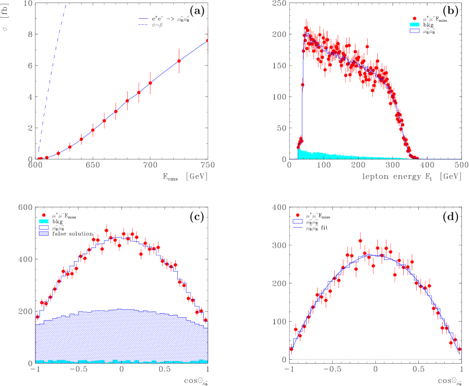
Figure 5: (a) The unpolarized cross section of $e^{+}e^{-}\to{\tilde{\mu}_{R}}^{+}{\tilde{\mu}_{R}}^{-}$ production close to threshold, including QED radiation, beamstrahlung and width effects; the statistical errors correspond to ${\cal L}=10\,\mathrm{fb}^{-1}$ per point, the dash-dotted curve indicates, with the same coefficient, the hypothetical dependence $\sigma\sim\beta$ instead of $\sigma\sim{\beta^{3}}$; (b) energy spectrum $E_{\mu}$ from ${\tilde{\mu}_{R}}^{-}\to\mu^{-}{\tilde{\chi}^{0}}_{1}$ decays; polar angle distribution $\cos\theta_{\tilde{\mu}_{R}}$ (c) with and (d) without contribution of false solution. The simulation for the energy and polar angle distribution is based on polarized beams with $({\cal P}_{e^{-}},{\cal P}_{e^{+}})=(+0.8,-0.6)$ at $\sqrt{s}=1\,\mathrm{TeV}$ and ${\cal L}=500\,\mathrm{fb}^{-1}$. The smooth histograms represent high statistics expectations, the curve indicates a fit to the cross section (2.5).

The unpolarized cross section as a function of energy close to the production threshold, including all instrumental effects, is shown in Fig. 5(a). The remaining flat background from $W^{+}W^{-}$ production (not shown) amounts to about $0.5\;\mathrm{fb}$, and it can be subtracted by extrapolation from the sideband below. The excitation curve exhibits a slow rise as expected from the characteristic dependence $\sigma_{{\tilde{\mu}_{R}}{\tilde{\mu}_{R}}}\sim\beta^{3}$ explained in Eq. (2.7). Such a behavior can be clearly distinguished from a much steeper hypothetical $S$-wave dependence $\sigma\sim\beta$, shown as well for comparison.

The ${\tilde{\mu}_{R}}^{\pm}$ angular distribution is investigated in the continuum choosing an energy of $\sqrt{s}=1\;\mathrm{TeV}$ and an integrated luminosity of ${\cal L}=500\,\mathrm{fb}^{-1}$. In order to enhance the signal and suppress SUSY and SM background processes, the beams are assumed to be polarized with values of $({\cal P}_{e^{-}},{\cal P}_{e^{+}})=(+0.8,-0.6)$, resulting in a cross section of $30\;\mathrm{fb}$.

The spectrum of the muon energy $E_{\mu}$ is shown in Fig. 5(b). The signal is very clean above the very low background from SUSY and $W^{+}W^{-}$ production, which gets reduced further to $\sim 1.3\;\%$ after reconstruction of the kinematics. The primary flat energy spectrum, characteristic for a spin 0 particle decay, is distorted due to acceptance cuts, event selection criteria and photon radiation. However, the minimal and maximal endpoint energies $E_{\pm}$ are clearly pronounced. The polar angle distribution of the smuons ${\tilde{\mu}_{R}}$, including both the correct and false solutions, is displayed in Fig. 5(c). The tiny background gives a flat contribution. The false solution exhibits a large pedestal with some enhancement in the central region reflecting mildly the primary distribution (cf. $\beta=0.8$). The ambiguous solution can be calculated using Monte Carlo simulation and it is subtracted in Fig. 5(d). The expected $\sin^{2}\theta$ distribution of Eq. (2.8) is clearly visible. A fit of the shape to the experimental angular distribution yields

$$\mbox{ }\hskip 28.45274pt\frac{d\sigma^{\rm exp}}{d\cos\theta}\,\sim\,1+a\cos\theta+b\cos^{2}\theta$$ (2.35)

$$a=-0.020\pm 0.016\quad\mbox{and}\quad b=-0.979\pm 0.022$$

confirming the conjectured forward-backward symmetric $\sin^{2}\theta$ behavior of spin-0 smuon production with high precision.

3 SELECTRONS

3.1 Production Channels in $e^{+}e^{-}$ Collisions

In the selectron production process the lepton number can flow from the initial to the final state. Therefore, besides the $e^{+}e^{-}$ annihilation channel mediated by $\gamma,Z$ exchange, cf. Fig. 1(a), also $t$-channel exchange of neutralinos, cf. Fig. 1(b), contributes to some channels. [In $e^{-}e^{-}$ collisions selectrons are produced solely by $t$-channel and $u$-channel exchanges.] Among all these channels, which are summarized comprehensively in Table 1 of Ref. [17], pair production of $\tilde{e}^{+}_{R}\tilde{e}^{-}_{R}$ is easiest to control experimentally if, as realized in many models, the R-type selectron is significantly lighter than the companion L-type selectron. Equal-particle channels are also preferred theoretically; their analysis is most transparent by including the standard annihilation which is well controlled.

Two electron/positron polarization states can generate the $\tilde{e}^{+}_{R}\tilde{e}^{-}_{R}$ pair:

$$e^{+}_{R}\,e^{-}_{L}\ \ \to\ \ \tilde{e}^{+}_{R}\,\tilde{e}^{-}_{R}\qquad\quad[\gamma,Z\ \ \mbox{exchange}]$$ (3.1)

$$e^{+}_{L}\,e^{-}_{R}\ \ \to\ \ \tilde{e}^{+}_{R}\,\tilde{e}^{-}_{R}\qquad\quad[\gamma,Z,\tilde{\chi}^{0}\ \ \mbox{exchange}]$$ (3.2)

Though the signal process (3.1) is the analogue of smuon pair production in $e^{+}e^{-}$ annihilation, we cannot anticipate that in rival $J=1/2,1,..$ processes $t$-channel exchanges do not occur when the lepton number can flow from the initial to the final state. Moreover, even electron polarization [32] can be realized only at a degree $<1$ so that impurities from the process are mixed in in any case. It is thus plausible to evaluate $\tilde{e}^{+}_{R}\tilde{e}^{-}_{R}$ pair production for unpolarized electron/positron beams. [The general expression of the polarized cross section is given in the Appendix.] This case exemplifies all the interesting characteristics.

After exploiting the conservation of the lepton current, the spinorial parts of the matrix elements for $s$-channel $\gamma,Z$ exchange and $t$-channel neutralino exchange are identical, $\,\sim\,(\bar{v}_{e^{+}}\gamma_{\mu}u_{e^{-}})\,k^{\mu}$ with $k^{\mu}$ denoting the (spacelike) 4-momentum transfer. The $t$-channel contribution can therefore be mapped into generalized charges, introduced in analogy to Eqs. (2.2) and (2.3):

$$Q_{L}=1+\left(s^{2}_{W}-1/2\right)c^{-2}_{W}D_{Z}(s)$$ (3.3)

$$Q_{R}=1+t^{2}_{W}D_{Z}(s)+\sum^{4}_{k=1}|N_{k1}|^{2}c^{-2}_{W}D_{\tilde{\chi}^{0}_{k}}(t)$$ (3.4)

The indices $R$ and $L$ denote the electron helicities. The pole part of the $\tilde{\chi}^{0}_{k}$ propagator, $k=1,..,4$ in the Minimal Supersymmetric Standard Model (MSSM), is denoted in the center-of-mass frame by

$$D_{\tilde{\chi}^{0}_{k}}(t)\equiv\frac{s}{t-m^{2}_{\tilde{\chi}^{0}_{k}}}=\frac{-2}{\Delta_{k}-\beta_{\tilde{e}_{R}}\cos\theta}\quad\mbox{with}\quad\Delta_{k}=1-2(m^{2}_{\tilde{e}_{R}}-m^{2}_{\tilde{\chi}^{0}_{k}})/s$$ (3.5)

while $N$ denotes the neutralino mixing matrix, see Ref. [33]. Near the threshold, the $\tilde{e}^{+}_{R}\tilde{e}^{-}_{R}$ pair is produced in a $P$-wave with amplitude $\sim\beta$. With rising energy however an increasing number of orbital angular momenta is excited and the propagator starts diverging in the forward direction $\sim s/m^{2}_{\tilde{\chi}^{0}_{k}}$ [for $m_{\tilde{e}_{R}}>m_{\tilde{\chi}^{0}_{k}}$ after running through a maximum at $\cos\theta\sim\Delta_{k}/\beta_{\tilde{e}_{R}}$].

The differential and total cross sections can be cast into the form

$$\frac{d\sigma}{d\cos\theta}[e^{+}e^{-}\to\tilde{e}^{+}_{R}\tilde{e}^{-}_{R}] = \frac{\pi\alpha^{2}}{8s}\beta^{3}\sin^{2}\theta\left[Q^{2}_{L}+Q^{2}_{R}\right]$$ (3.6)

$$\sigma[e^{+}e^{-}\to\tilde{e}^{+}_{R}\tilde{e}^{-}_{R}] = \frac{\pi\alpha^{2}}{8s}\beta^{3}\left[\langle Q^{2}_{L}\sin^{2}\theta\rangle+\langle Q^{2}_{R}\sin^{2}\theta\rangle\right]$$ (3.7)

with $\langle Q^{2}_{L,R}\sin^{2}\theta\rangle\equiv\int d\cos\theta\,\sin^{2}\theta\,Q^{2}_{L,R}$. Mass and energy dependence of the integrated charges can be adopted from Ref. [17]:

$$\langle Q^{2}_{L}\sin^{2}\theta\rangle = \frac{4}{3}\left[1+(s^{2}_{W}-1/2)c^{-2}_{W}D_{Z}(s)\right]^{2}$$ (3.8)

$$\langle Q^{2}_{R}\sin^{2}\theta\rangle = \frac{4}{3}\,[1+t^{2}_{W}D_{Z}(s)]^{2}+8[1+t^{2}_{W}D_{Z}(s)]c^{-2}_{W}\sum^{4}_{j=1}|N_{j1}|^{2}f^{j}$$ (3.9)

$$\;\;\;\;+8c^{-4}_{W}\sum^{4}_{j,k=1}|N_{j1}N_{k1}|^{2}h^{jk}$$

with the coefficients

$$f^{j}=-\beta\Delta_{j}+\frac{\Delta^{2}_{j}-\beta^{2}}{2}\ln\frac{\Delta_{j}+\beta}{\Delta_{j}-\beta}\qquad\mbox{and}\qquad h^{jk}=\left\{\begin{array}[]{ll}-2\beta+\Delta_{j}\ln\frac{\Delta_{j}+\beta}{\Delta_{j}-\beta}&\,j=k\\[5.69054pt] (f^{j}-f^{k})/(\Delta_{j}-\Delta_{k})&\,j\neq k\end{array}\right.$$ (3.12)

It follows that the production of $e$-type supersymmetric scalar particles is characterized by the following two rules:

$$\#1 \ \ \sim\ \ \beta^{3}$$ threshold excitation (3.13)

$$\#2 \ \ \sim\ \ \sin^{2}\theta\,\,\mathcal{G}(\cos\theta)$$ angular distribution (3.14)

$$\ \ \rightarrow\ \ \sin^{2}\theta\ \ \mbox{near threshold}$$

Independent of energy, the angular distribution must behave $\sim\sin^{2}\theta$ close to the forward and backward directions where it must vanish by angular momentum conservation. While this behavior may be masked in practice by the singularity in $\mathcal{G}$ developing in the forward direction at high energies, no such interference will arise in the backward direction. Since the $\tilde{\chi}^{0}_{k}$ exchanges give rise to a $P$-wave near the threshold, in the same way as $\gamma,Z$ exchange, a simple picture with $\sigma\sim\beta^{3}$ and $d\sigma/d\cos\theta\sim\sin^{2}\theta$ emerges at the threshold.

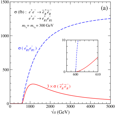
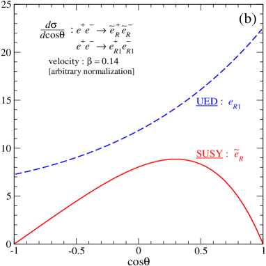
Figure 6: (a) The threshold excitation for selectrons; and (b) the angular distribution in $e^{+}e^{-}\to\tilde{e}^{+}_{R}\tilde{e}^{-}_{R}$ for the SUSY parameters specified in the text. These results are compared with the production $e^{+}e^{-}\to e^{+}_{R1}e^{-}_{R1}$ of electronic Kaluza-Klein states in UED. The first KK mass $M_{K_{1}}$ is taken to be 295 GeV.

Asymptotically the total cross section scales as

$$\sigma\ \ \to\ \ \frac{\pi\alpha^{2}}{c_{W}^{4}}\,\,\frac{1}{s}\,\log{\frac{s}{m^{2}_{\tilde{e}_{R}}}}\quad\mbox{for}\quad s\ \ \rightarrow\ \ \infty$$ (3.15)

as expected from the forward enhancement of the $t$-channel exchange.

These characteristics are displayed quantitatively in Fig. 6(a/b) for the onset of the excitation curve and the angular distribution close to threshold.

3.2 KK Excited States $e^{\pm}_{1}$ in UED

The analysis presented above repeats itself rather closely for the KK excited states carrying electron lepton number; again we choose the first KK excited R-type electrons $e^{\pm}_{R1}$ with vector couplings to not only $\gamma$ and but also to $Z$ bosons as a representative example:

$$e^{+}e^{-}\ \ \rightarrow\ \ e^{+}_{R1}e^{-}_{R1}$$ (3.16)

Analogously to Fig. 1(b), the $t$-channel exchange of the vector and scalar KK excitations $B_{1}$ and $b_{1}$ [the supplement left with $B_{1}$ from the 5-dimensional vector] add to the standard $\gamma,Z$ exchanges corresponding to Fig. 1(a).

Despite the complicated superposition of vector and scalar interactions, Fierzing techniques allow us to cast all contributions into the $s$-channel $\gamma_{\mu}\otimes\gamma_{\mu}$ form for the chiral $\alpha,\beta=L,R$ elements:

$${\cal M}[e^{+}e^{-}\to e^{+}_{R1}e^{-}_{R1}]=Q^{1}_{\alpha\beta}\left[\bar{v}(e^{+})\gamma_{\mu}P_{\alpha}u(e^{-})\right]\left[\bar{u}(e^{-}_{R1})\gamma^{\mu}P_{\beta}v(e^{+}_{R1})\right]$$ (3.17)

with the bilinear charges [34]:

$$\begin{array}[]{ll}Q^{1}_{LL}=1+\left(s^{2}_{W}-1/2\right)c^{-2}_{W}D_{Z}(s),&Q^{1}_{LR}=Q^{1}_{LL}-\frac{1}{8}\frac{m^{2}_{Z}}{M^{2}_{K_{1}}+m^{2}_{Z}}t^{2}_{W}D_{b_{1}}(t)\\[5.69054pt] Q^{1}_{RL}=1+t^{2}_{W}D_{Z}(s)+c_{W}^{-2}\frac{m^{2}_{e_{R1}}}{2M^{2}_{K_{1}}}D_{B_{1}}(t),&Q^{1}_{RR}=1+t^{2}_{W}D_{Z}(s)+c^{-2}_{W}D_{B_{1}}(t)\end{array}$$ (3.20)

Apart from standard notations, $M_{K_{1}}$ denotes the first KK mass, and the $t$-channel propagators are defined as $D_{B_{1}}(t)=D_{b_{1}}(t)=s/[t-M^{2}_{K_{1}}]=-2/[1-2(m^{2}_{e_{R1}}-M^{2}_{K_{1}})/s-\beta_{e_{R1}}\cos\theta]$.

After introducing the familiar quartic charges

$$Q^{1}_{1}=\frac{1}{4}\left[|Q^{1}_{RR}|^{2}+|Q^{1}_{LL}|^{2}+|Q^{1}_{RL}|^{2}+|Q^{1}_{LR}|^{2}\right]$$

$$Q^{1}_{2}=\frac{1}{2}\Re{\rm e}\left[Q^{1}_{RR}Q^{1*}_{RL}+Q^{1}_{LL}Q^{1*}_{LR}\right]$$

$$Q^{1}_{3}=\frac{1}{4}\left[|Q^{1}_{RR}|^{2}+|Q^{1}_{LL}|^{2}-|Q^{1}_{RL}|^{2}-|Q^{1}_{LR}|^{2}\right]$$ (3.21)

the differential cross section can be written in the compact form

$$\frac{d\sigma}{d\cos\theta}\,[e^{+}e^{-}\to e^{+}_{R1}e^{-}_{R1}]=\frac{\pi\alpha^{2}}{2s}\beta\bigg{[}(1+\beta^{2}\cos^{2}\theta)Q^{1}_{1}+(1-\beta^{2})Q^{1}_{2}+2\beta\cos\theta Q^{1}_{3}\bigg{]}$$ (3.22)

from which the total cross section follows by integration over the polar angle:

$$\sigma[e^{+}e^{-}\to e^{+}_{R1}e^{-}_{R1}]=\frac{\pi\alpha^{2}}{2s}\beta\bigg{[}\langle Q^{1}_{1}\rangle+\beta^{2}\langle\cos^{2}\theta Q^{1}_{1}\rangle+(1-\beta^{2})\langle Q^{1}_{2}\rangle+2\beta\langle\cos\theta Q^{1}_{3}\rangle\bigg{]}$$ (3.23)

Both observables can serve as discriminants for Kaluza-Klein states against supersymmetric selectrons.

By inspecting the cross sections in Eqs. (3.23) and (3.22) we can easily conclude, without studying details, that

$$\sigma[e^{+}e^{-}\to e^{+}_{R1}e^{-}_{R1}] \sim \beta\ \ \mbox{near threshold}$$ (3.24)

$$\frac{d\sigma}{d\cos\theta}\,[e^{+}e^{-}\to e^{+}_{R1}e^{-}_{R1}] \sim (1+\beta^{2}\cos^{2}\theta)\,\mathcal{G}(\cos\theta)+\cdots$$ (3.25)

$$\rightarrow \cos\theta$$ flat in near threshold

as generally expected for fermion pair production near the threshold. As for smuon pairs, these results contrast strongly to supersymmetric scalar $\tilde{e}$ production. Most striking is the non-vanishing angular distribution in the forward and backward directions. This is exemplified quantitatively in the comparison of Fig. 6(a/b).

Asymptotically however the total cross section, unlike the previous examples, approaches a non-zero value

$$\sigma\ \ \to\ \ \frac{\pi\alpha^{2}}{c_{W}^{4}}\,\frac{1}{M^{2}_{K_{1}}}\quad\mbox{for}\quad s\ \ \rightarrow\ \ \infty$$ (3.26)

due to the enhancement in the forward direction, which is a remnant of the Rutherford pole damped by the Yukawa mass cut-off in the exchange of heavy particles.

3.3 General Analysis

Independent of the lepton number flow by additional $t$-channel exchange mechanisms, the $s$-channel $\gamma,Z$ exchange in the production of charged fermions of any spin $J=1/2,3/2,\ldots$ will generate the pair in an $S$-wave so that the cross section should rise at threshold $\sim\beta$ in contrast to the scalar $\beta^{3}$ particle production. The same $\gamma,Z$ exchange mechanism will generate a non-vanishing angular distribution in the forward and backward directions $\neq\sin^{2}\theta$.

In contrast to the production of muon-type pairs, the additional $t$-channel exchanges in the production of $J=1,2,..$ integer spin electron-type pairs will in general give rise to an $S$-wave component $\sim\beta$ in the onset of the excitation curve. Since all spin $J>0$ particles in asymptotically well-behaved field theories [19] will carry a non-vanishing magnetic dipole moment, the angular distribution for both muon-type and electron-type pairs will not vanish in forward/backward direction. This argument can be supplemented by studying the polarizations $\sim d^{J}_{\lambda,\sigma}(\theta^{*})$ in the decays of the two spin $J$ particles.

Thus in parallel to the smuon case, also for selectrons in supersymmetric theories experimental paths can be designed for establishing the scalar spin-0 character unambiguously.

3.4 Simulation of $e^{+}e^{-}\to{\tilde{e}_{R}}^{+}{\tilde{e}_{R}}^{-}$

The detection of scalar selectrons in the reaction $e^{+}e^{-}\to{\tilde{e}_{R}}^{+}{\tilde{e}_{R}}^{-}\to e^{+}{\tilde{\chi}^{0}}_{1}\,e^{-}{\tilde{\chi}^{0}}_{1}$ is again very clean. The event simulation, selection and analysis proceed in complete analogy to smuon production, described in the previous section, just replacing the observable leptons by an $e^{+}e^{-}$ pair.

Figure 7: (a) The unpolarized cross section of $e^{+}e^{-}\to{\tilde{e}_{R}}^{+}{\tilde{e}_{R}}^{-}$ production close to threshold, including QED radiation, beamstrahlung and width effects; the statistical errors correspond to ${\cal L}=10\,\mathrm{fb}^{-1}$ per point, the dash-dotted curve indicates a hypothetical dependence $\sigma\sim\beta$; (b) energy spectrum $E_{e}$ from ${\tilde{e}_{R}}^{\pm}\to e^{\pm}{\tilde{\chi}^{0}}_{1}$ decays; polar angle distribution $\cos\theta_{\tilde{e}_{R}}$ (c) with and (d) without contribution of false solution. The simulation for the energy and polar angle distributions is based on polarized beams with $({\cal P}_{e^{-}},{\cal P}_{e^{+}})=(+0.8,-0.6)$ at $\sqrt{s}=680\,\mathrm{GeV}$ and ${\cal L}=200\,\mathrm{fb}^{-1}$. The smooth histograms represent high statistics expectations, the curve indicates a fit to the cross section (3.6).

The unpolarized cross section at threshold is displayed in Fig. 7(a). The expected event rates are larger than for smuon production due to additional $t$-channel neutralino exchange. One observes a cross section typical for $P$-wave production of spin-0 particles with a dependence $\sigma_{{\tilde{e}_{R}}^{+}{\tilde{e}_{R}}^{-}}\sim\beta^{3}$, as explained in Eq. (3.13). The excitation curve may be easily distinguished from a much faster rising hypothetical $\sigma\sim\beta$ behavior, shown for comparison as well.

The study of the ${\tilde{e}_{R}}^{+}{\tilde{e}_{R}}^{-}$ production is performed close to threshold in order to separate out, as well as possible, the factor $\sin^{2}\theta$ in the polar-angle distribution, see Eq. (3.14). An energy of $\sqrt{s}=680\,\mathrm{GeV}$ appears to be a good compromise between signal and background event rates. An enhanced signal is obtained by choosing beam polarizations of $({\cal P}_{e^{-}},{\cal P}_{e^{+}})=(+0.8,-0.6)$. The cross section amounts to $47\,\mathrm{fb}$, and an integrated luminosity of ${\cal L}=200\,\mathrm{fb}^{-1}$ is assumed for the simulation. The expected electron energy spectrum $E_{e}$ of the decays ${\tilde{e}_{R}}^{\pm}\to e^{\pm}{\tilde{\chi}^{0}}_{1}$ is shown in Fig. 7(b). It exhibits a clear signature above a negligible background from $W^{+}W^{-}$ and ${\tilde{e}_{R}}^{\pm}{\tilde{e}_{L}}^{\mp}$ production.

The angular distribution $\cos\theta_{\tilde{e}_{R}}$, shown in Fig. 7(c), is still peaked towards the forward direction, due to the remnant $t$-channel $\tilde{\chi}^{0}$ contributions, above a fairly constant pedestal from the false solutions. The spectrum after subtracting the ambiguity, displayed in Fig. 7(d), vanishes in the very forward and backward directions, reflecting the overall $\sin^{2}\theta$ factor. A fit according to the differential cross section formula (3.6) yields a very good description of the simulated data. As a by-product, the results of the fit can be used to determine or cross-check the neutralino mixing parameters $|N_{k1}|^{2}$ entering the expression (3.4) of the generalized charge $Q_{R}$.

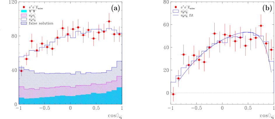
Figure 8: Polar angle distribution $\cos\theta_{\tilde{e}_{R}}$ of $e^{+}_{R}e^{-}_{L}\to{\tilde{e}_{R}}^{+}{\tilde{e}_{R}}^{-}$: (a) with contributions from background and false solution; (b) after subtraction of background and false solution. The simulation is based on polarized beams with $({\cal P}_{e^{-}},{\cal P}_{e^{+}})=(-0.8,+0.6)$ at $\sqrt{s}=680\,\mathrm{GeV}$ and ${\cal L}=300\,\mathrm{fb}^{-1}$. The smooth histograms represent high statistics expectations, the curve indicates a fit to the cross section (3.6)

The $t$-channel neutralino exchange can be considerably reduced by choosing opposite beam polarizations of $({\cal P}_{e^{-}},{\cal P}_{e^{+}})=(-0.8,+0.6)$. These conditions however imply a much lower cross section of $\sigma=3.4\,\mathrm{fb}$ at the same energy $\sqrt{s}=680\,\mathrm{GeV}$ and a significantly larger background from $WW$ and ${\tilde{e}_{R}}{\tilde{e}_{L}}$ production. The results of simulations assuming ${\cal L}=300\,\mathrm{fb}^{-1}$ are displayed in Fig. 8. The polar angle distribution is much flatter and shifted towards the central region, approaching the expected $\sin^{2}\theta$ law for completely polarized beams. A fit to the subtracted spectrum exhibits a skewed $\sin^{2}\theta$ distribution, reminiscent of small, residual $t$–channel contributions.

4 CHARGINOS AND NEUTRALINOS

4.1 Production Channels in $e^{+}e^{-}$ Collisions

The prototypes of non-colored supersymmetric spin-1/2 fermions are the charginos $\tilde{\chi}^{\pm}_{1}$ and the neutralinos $\tilde{\chi}^{0}_{1}$ and $\tilde{\chi}^{0}_{2}$. They are produced in diagonal and mixed pairs in $e^{+}e^{-}$ annihilation:

$$e^{+}e^{-}\rightarrow\tilde{\chi}^{+}_{1}\tilde{\chi}^{-}_{1}\hskip 82.51282pt\mbox{with}\ \ \ \ \tilde{\chi}^{\pm}_{1}\rightarrow f\bar{f}^{\prime}\tilde{\chi}^{0}_{1}$$ (4.1)

$$e^{+}e^{-}\rightarrow\tilde{\chi}^{0}_{1}\tilde{\chi}^{0}_{2}\ \ \mbox{and}\ \ \tilde{\chi}^{0}_{2}\tilde{\chi}^{0}_{2}\hskip 31.2982pt\mbox{with}\ \ \ \ \tilde{\chi}^{0}_{2}\rightarrow f\bar{f}\tilde{\chi}^{0}_{1}$$ (4.2)

Though a significant fraction of the decays is mediated potentially by $\tilde{\tau}$ intermediate states as predicted in the reference scenarios SPS1a/1a^′ [35, 18, 36], other decay modes can still play a significant r$\hat{\rm o}$le due to large production cross sections, in particular for diagonal pairs. The mixed neutralino production channel $\tilde{\chi}^{0}_{1}\tilde{\chi}^{0}_{2}$ is easier to analyze in the threshold region when studying the onset of the excitation curve, but the diagonal pair $\tilde{\chi}^{0}_{2}\tilde{\chi}^{0}_{2}$ gives rise to a better textured visible final state that allows the reconstruction of the flight axis up to a 2-fold ambiguity, while the axis can be reconstructed for mixed pairs only if $\tilde{\chi}^{0}_{2}$ cascades down through an intermediate slepton [37].

Figure 9: Two mechanisms contributing to the production of $\tilde{\chi}^{+}_{1}\tilde{\chi}^{-}_{1}$ and three to $\tilde{\chi}^{0}_{1}\tilde{\chi}^{0}_{2}$ and $\tilde{\chi}^{0}_{2}\tilde{\chi}^{0}_{2}$; $s$-channel $\gamma/Z$ exchanges and $t/u$-channel $\tilde{\nu}$ and $\tilde{e}$ exchanges, respectively.

Two mechanisms contribute to the production of $\tilde{\chi}^{+}_{1}\tilde{\chi}^{-}_{1}$ and three to $\tilde{\chi}^{0}_{1}\tilde{\chi}^{0}_{2}$ and $\tilde{\chi}^{0}_{2}\tilde{\chi}^{0}_{2}$: $s$-channel $\gamma/Z$ exchanges and $t/u$-channel $\tilde{\nu}$ and $\tilde{e}$ exchanges, respectively, as illustrated in Fig. 9.

By using Fierzing techniques, both the $t/u$-channel diagrams can be mapped onto the $s$-channel diagram, generating the bilinear charges $Q_{\alpha\beta}$ [38, 33]:

$$\begin{array}[]{lll}\mbox{\framebox{$\tilde{\chi}^{+}_{1}\tilde{\chi}^{-}_{1}$}}:&Q_{LL}=D_{L}-F_{L}\cos 2\phi_{L}&Q_{LR}=D^{\prime}_{L}-F^{\prime}_{L}\cos 2\phi_{R}\\ {}&Q_{RL}=D_{R}-F_{R}\cos 2\phi_{L}&Q_{RR}=D_{R}-F_{R}\cos 2\phi_{R}\end{array}$$ (4.5)

$$\begin{array}[]{ll}\mbox{\framebox{$\tilde{\chi}^{0}_{i}\,\,\tilde{\chi}^{0}_{j}$}}:&Q_{LL}=+4{\cal Z}_{ij}s^{-2}_{2W}(s^{2}_{W}-1/2)D_{Z}(s)-{\cal G}_{Lij}D_{\tilde{e}_{L}}(u)\\ {}&Q_{LR}=-4{\cal Z}^{*}_{ij}s^{-2}_{2W}(s^{2}_{W}-1/2)D_{Z}(s)+{\cal G}^{*}_{Lij}D_{\tilde{e}_{L}}(t)\\ {}&Q_{RL}=+{\cal Z}_{ij}c^{-2}_{W}D_{Z}(s)+{\cal G}_{Rij}D_{\tilde{e}_{R}}(t)\\ {}&Q_{RR}=-{\cal Z}^{*}_{ij}c^{-2}_{W}D_{Z}(s)-{\cal G}^{*}_{Rij}D_{\tilde{e}_{R}}(u)\end{array}$$ (4.10)

[in the usual notation $s^{2}_{2W}=\sin^{2}2\theta_{W}$]. The normalized propagators in these charges read

$$D_{L}=1+4s^{-2}_{2W}(s^{2}_{W}-1/2)(s^{2}_{W}-3/4)D_{Z}(s)\qquad F_{L}=4s^{-2}_{2W}(s^{2}_{W}-1/2)D_{Z}(s)/4$$

$$D_{R}=1+c^{-2}_{W}(s^{2}_{W}-3/4)D_{Z}(s)\hskip 82.51282ptF_{R}=c^{-2}_{W}D_{Z}(s)/4$$

$$D^{\prime}_{L}=D_{L}+s^{-2}_{W}D_{\tilde{\nu}}(t)/4\hskip 119.50148ptF^{\prime}_{L}=F_{L}-s^{-2}_{W}D_{\tilde{\nu}}(t)/4$$ (4.11)

and $\phi_{L,R}$ denote the mixing angles rotating the gaugino/higgsino current to the chargino mass basis; the rotation angles are determined by the SUSY Lagrangian parameters $M_{2},\mu$ and $\tan\beta$ [38]. The matrices ${\cal Z}$ and ${\cal G}_{L,R}$ are combinations of the mixing matrix elements $N$ in the neutralino sector [33]:

$${\cal Z}_{ij}=(N_{i3}N^{*}_{j3}-N_{i4}N^{*}_{j4})/2$$

$${\cal G}_{Lij}=(N_{i2}c_{W}+N_{i1}s_{W})(N^{*}_{j2}c_{W}+N^{*}_{j1}s_{W})/s^{2}_{2W}$$

$${\cal G}_{Rij}=N_{i1}N^{*}_{j1}/c^{2}_{W}$$ (4.12)

They are derived from the Lagrangian parameters noted above and supplemented by the U(1) gaugino parameter $M_{1}$ [in the MSSM].

Defining the quartic charges $Q_{1},Q_{2},Q_{3}$ in the same way as Eq. (3.21), the differential and total cross sections can be written as

$$\!\!\!\!\!\!\!\!\!\frac{d\sigma}{d\cos\theta}\! = \!\frac{\pi\alpha^{2}}{2s}\beta\left\{[1-(\mu^{2}_{i}-\mu^{2}_{j})^{2}+\beta^{2}\cos^{2}\theta]Q_{1}+4\mu_{i}\mu_{j}Q_{2}+2\beta\cos\theta Q_{3}\right\}$$ (4.13)

$$\!\!\!\!\!\!\!\!\!\sigma\! = \!\frac{\pi\alpha^{2}f_{s}}{2s}\beta\left\{[1-(\mu^{2}_{i}-\mu^{2}_{j})]\langle Q_{1}\rangle+\beta^{2}\langle\cos^{2}\theta\,Q_{1}\rangle+4\mu_{i}\mu_{j}\langle Q_{2}\rangle+2\beta\langle\cos\theta\,Q_{3}\rangle\right\}$$ (4.14)

generically for any pair of masses with $\mu_{i}=m_{i}/\sqrt{s}$, and $\beta^{2}=[1-(\mu_{i}-\mu_{j})^{2}][1-(\mu_{i}+\mu_{j})^{2}]$ coinciding with the velocity squared for equal masses; $f_{s}=1$ or $1/2$ denotes the statistics factor for pairs of unequal and equal particles, respectively, in the final state.

(a) Charginos:
Near the threshold the cross section rises $\sim\beta$ since the charged Dirac particles are generated in $S$-waves. For asymptotic energies the cross section scales as

$$\sigma\ \ \to\ \ \frac{4\pi\alpha^{2}}{3s}\,\left(1+\Delta_{\tilde{\chi}^{\pm}}\right)\quad\mbox{for}\quad s\ \ \rightarrow\ \ \infty$$ (4.15)

complemented by the coefficient $\Delta_{\tilde{\chi}^{\pm}}={\mathcal{O}}(1)$ including mixing matrix elements.

The angular distribution near the threshold is flat and need not vanish as for scalar particles in the forward/backward direction. With rising energy the sneutrino $t$-channel exchange excites an increasing number of higher orbital angular momenta and thus modifies the familiar spin-$1/2$ asymptotic distribution to $\sim(1+\cos^{2}\theta)\,{\cal G}(\cos\theta)$.

The characteristics for supersymmetric chargino production can therefore be summarized in the following points:

$$\#1\quad\mbox{threshold excitation}\ \ \sim\ \ \beta$$ (4.17)

$$\#2\quad\mbox{angular distribution}\ \ \sim\ \ (1+\beta^{2}\cos^{2}\theta)\,\mathcal{G}(\cos\theta)+\cdots$$

$$\rightarrow\ \ \mbox{isotropic near threshold}$$

As will be argued later, these two characteristics can be mimicked by higher half-integer spin states. Thus, the observation of the characteristics (4.17) and (4.17) is necessary for chargino spin assignments in supersymmetric theories but not sufficient. The production characteristics must be complemented by decay characteristics to determine the spin of charginos unambiguously.

(b) Neutralinos:
The Majorana nature of the neutralinos forbids the $S$-wave production of the diagonal $\tilde{\chi}^{0}_{2}\tilde{\chi}^{0}_{2}$ pair at threshold with equal spin components along the $e^{+}e^{-}$ beam axis as a consequence of the Pauli principle. This conclusion can also formally be drawn by observing that near threshold the sum of the quartic charges is reduced to $Q_{1}+Q_{2}=[|Q_{LL}+Q_{LR}|^{2}+|Q_{RL}+Q_{RR}|^{2}$]/4 so that the final-state current becomes purely vectorial, forbidden however for neutralino Majorana fields which can only be coupled to axial-vector currents. The $P$-wave production mode leads to the onset of the excitation curve $\sim\beta^{3}$. The angular distribution follows the spin-1 rule for $\gamma/Z$ exchange [39], modified however by a spin-1 and spin-0 mixture from selectron $t/u$ exchanges. Inserting the quartic charges in Eq. (4.13), the angular distribution is given near the threshold by

$$\frac{d\sigma_{thr}}{d\cos\theta}=\frac{\pi\alpha^{2}}{4s}\,\beta^{3}\,\sum_{k=L,R}\bigg{[}\!{\cal Z}^{2}_{k}(1+\cos^{2}\theta)+4\tilde{g}_{k}(2\tilde{g}_{k}-{\cal Z}_{k})\sin^{2}{\theta}+8\delta_{k}\tilde{g}_{k}(\delta_{k}\tilde{g}_{k}+{\cal Z}_{k})\cos^{2}\theta\,\bigg{]}$$ (4.18)

where the coefficients are defined in terms of the matrices ${\cal Z}$ and ${\cal G}_{L,R}$ as

$${\cal Z}_{R}={\cal Z}c^{-2}_{W}D_{Z}\hskip 89.626pt\tilde{g}_{R}={\cal G}_{R}\,[1+\delta_{R}]$$ (4.19)

$${\cal Z}_{L}=4{\cal Z}s^{-2}_{2W}(1/2-s^{2}_{W})D_{Z}\qquad\ \ \tilde{g}_{L}={\cal G}_{L}[1+\delta_{L}]$$ (4.20)

with $\delta_{L,R}=(m^{2}_{\tilde{\chi}^{0}_{2}}-m^{2}_{\tilde{e}_{L,R}})/(m^{2}_{\tilde{\chi}^{0}_{2}}+m^{2}_{\tilde{e}_{L,R}})$. For large selectron masses the $s$-channel $Z$ contributions are dominant and the angular distribution is reduced to $(1+\cos^{2}\theta)$, characteristic for Majorana fermion pair production. However, if for particle masses of the same size, the $t-$ and $u-$channel selectron contributions are dominant, the angular distribution is in general a mixture of $\sin^{2}\theta$ and $\cos^{2}\theta$ terms with coefficients varying with the particle masses. Above the threshold, higher orbital angular momenta are excited by the selectron exchange mechanisms, not altering however the asymptotic behavior

$$\sigma\ \ \to\ \ \frac{4\pi\alpha^{2}}{3s}\,\Delta_{\tilde{\chi}^{0}}\quad\mbox{for}\quad s\ \ \rightarrow\ \ \infty$$ (4.21)

with the coefficient $\Delta_{\tilde{\chi}^{0}}={\mathcal{O}}(1)$.

Also mixed $\tilde{\chi}^{0}_{1}\tilde{\chi}^{0}_{2}$ pairs will be produced near the threshold in a $P$-wave if their CP parities, $\pm i$, are equal. If they are different however $S$-wave production is possible and the cross section rises $\sim\beta$. In theories with CP violation $S$-wave production is predicted in general [33, 40].

These observations are summarized in the following rules:

$$\#1\quad\mbox{threshold excitation}\ \ \sim\ \ \beta^{3}\ \ \mbox{for}\ \ \tilde{\chi}^{0}_{2}\tilde{\chi}^{0}_{2}$$ (4.22)

$${}\hskip 120.35503pt\ \ \sim\ \ \beta^{3}/\beta\ \ \mbox{for}\ \ \tilde{\chi}^{0}_{1}\tilde{\chi}^{0}_{2}\ \ [\,\mbox{ident./diff. Majorana phases}\,]\ \$$

$$\#2\quad\mbox{angular distribution near threshold}\ \ \sim\ \ \cos^{2}/\sin^{2}\theta\;\mbox{mix}\$$ (4.23)

These points are illustrated for charginos and neutralinos in Figs. 10 and 11, respectively. The parameter set introduced earlier, gives rise to the chargino mass $m_{\tilde{\chi}^{\pm}_{1}}=$ 286 GeV and the neutralino masses $m_{\tilde{\chi}^{0}_{1/2}}=148/286$ GeV. The residual linear $\beta$-dependence, $\beta=0.14$, generates a slight increase of the angular distribution with $\cos\theta$. For neutralinos the chosen parameter set leads to a dominant $\sin^{2}\theta$ component in the angular distribution, supplemented however by small additional contributions, cf. Eq. (4.18), which render the distributions non-vanishing at the very edges of the forward and backward directions. These results will be confronted with phenomena in UED and a general analysis in the next subsections.

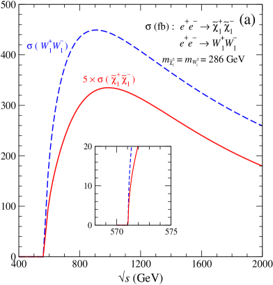
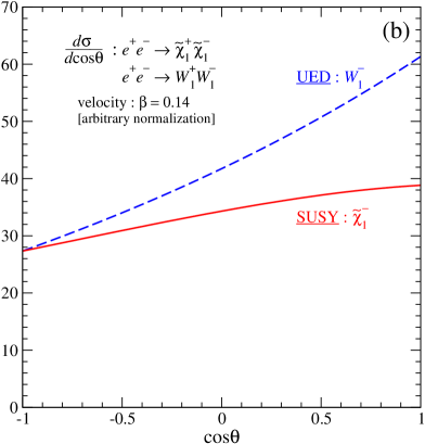
Figure 10: (a) The threshold excitation for charginos and (b) the angular distribution in the process $e^{+}e^{-}\to\tilde{\chi}^{+}_{1}\tilde{\chi}^{-}_{1}$ for the SUSY parameters specified in the text; both compared with $W^{+}_{1}W^{-}_{1}$ pair production in UED.

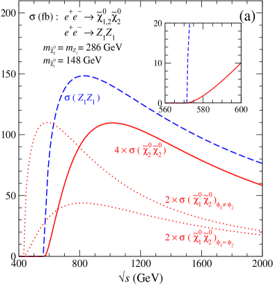
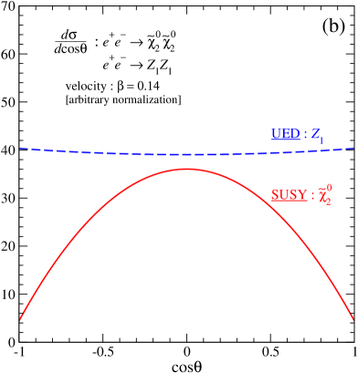
Figure 11: (a) The threshold excitation for neutralinos and (b) the angular distribution in the processes $e^{+}e^{-}\to\tilde{\chi}^{0}_{1}\tilde{\chi}^{0}_{2}$ and $\tilde{\chi}^{0}_{2}\tilde{\chi}^{0}_{2}$ for the SUSY parameters specified in the text; both compared with $Z_{1}Z_{1}$ pair production in UED.

4.2 KK Excited States $W^{\pm}_{1}$ and $Z_{1}/\gamma_{1}$ in UED

The counterpart of $\tilde{\chi}^{\pm}_{1}$ and $\tilde{\chi}^{0}_{2}$ in UED are the KK excitations $W^{\pm}_{1}$ and $W^{3}_{1}=Z_{1}$, while $\tilde{\chi}^{0}_{1}$ and $B_{1}=\gamma_{1}$ are the stable particles of the two theories with minimal mass to which all other particles cascade down.

Figure 12: Two mechanisms contributing to the production of $W^{+}_{1}W^{-}_{1}$ and two to $Z_{1}Z_{1}$; $s$-channel $\gamma/Z$ exchanges, $t$-channel $\nu_{1}$ and $t/u$-channel $e_{L1}$ exchanges, respectively.

The cross sections for the processes

$$e^{+}e^{-}\ \ \rightarrow\ \ W^{+}_{1}W^{-}_{1}$$ (4.24)

$$e^{+}e^{-}\ \ \rightarrow\ \ \,Z_{1}Z_{1}$$ (4.25)

are closely related to the corresponding SM processes $e^{+}e^{-}\to W^{+}W^{-}$ and $ZZ$, cf. Fig. 12. Standard SM couplings are attached to the currents, and the exchanged neutrino and electron must be substituted by the heavy KK excitations. In the limit in which the masses of the $t/u$-exchange leptons are neglected, the cross sections approach the SM form of Refs. [41, 42].

The differential and total cross sections for $W^{+}_{1}W^{-}_{1}$ can be expressed by the generalized charges

$$Q_{L}=1-(s^{2}_{W}-1/2)s^{-2}_{W}D_{Z}(s)\quad\ \ \mbox{and}\quad\ \ Q_{R}=1-D_{Z}(s)$$ (4.26)

In this notation they can be written as

$$\frac{d\sigma}{d\cos\theta}\! = \!\frac{\pi\alpha^{2}}{8s}\beta\left[s^{-4}_{W}F_{1}(s,\theta)+\frac{1}{2}(Q^{2}_{L}+Q^{2}_{R})\,F_{2}(s,\theta)-Q_{L}s_{W}^{-2}F_{3}(s,\theta)\right]$$ (4.27)

$$\sigma\! = \!\frac{\pi\alpha^{2}}{8s}\beta\left[s^{-4}_{W}\,\bar{\sigma}_{1}(s)+\frac{1}{2}(Q^{2}_{L}+Q^{2}_{R})\,\bar{\sigma}_{2}(s)-Q_{L}s_{W}^{-2}\,\bar{\sigma}_{3}(s)\right]$$ (4.28)

The angular functions $F(s,\theta)$ and the energy-dependent coefficients $\bar{\sigma}(s)$ are given by

$$F_{1}(s,\theta)=\frac{\gamma^{2}(1+\beta^{2}-2\beta\cos\theta)^{2}\,(4+\gamma^{2}\beta^{2}\sin^{2}\theta)+4\beta^{2}\sin^{2}\theta}{4(\Delta-\beta\cos\theta)^{2}}$$ (4.29)

$$F_{2}(s,\theta)=2\beta^{2}\left[4\gamma^{2}(4+\gamma^{2}\beta^{2}\sin^{2}\theta)+3\sin^{2}\theta\right]$$ (4.30)

$$F_{3}(s,\theta)=\frac{2\gamma^{2}\beta\,[2\beta-(1+\beta^{2})\cos\theta](4+\gamma^{2}\beta^{2}\sin^{2}\theta)+3\beta^{2}\sin^{2}\theta}{(\Delta-\beta\cos\theta)}$$ (4.31)

with $\gamma=\sqrt{s}/2m_{W^{\pm}_{1}}$, $\Delta=1-2(m^{2}_{W^{\pm}_{1}}-m^{2}_{\nu_{1}})/s$, and

$$\bar{\sigma}_{1}(s) = 4(\gamma^{4}+11\gamma^{2}-3)/3-(2\gamma^{2}-1)\eta^{2}-2\eta^{4}-2\left[\gamma^{-2}+2(2-\gamma^{-2})\eta^{2}\right]/(\Delta^{2}-\beta^{2})$$ (4.32)

$$+\left[4\Delta-(7+\Delta)\eta^{2}+(1+2\Delta)\eta^{4}\right]L(\bar{\beta})/\Delta$$

$$\bar{\sigma}_{2}(s) = 8\beta^{2}(4\gamma^{4}+20\gamma^{2}+3)/3$$ (4.33)

$$\bar{\sigma}_{3}(s) = 6\Delta+8(2\gamma^{4}+9\gamma^{2}-5)/3-[\gamma^{-2}+(2-\gamma^{-2})\eta^{2}]\,(2\gamma^{2}-1+\eta^{2})$$ (4.34)

$$-\left\{6(\Delta^{2}-\beta^{2})+\left[\gamma^{-2}+(2-\gamma^{-2})\eta^{2}\right]\left[7+\Delta-(1+\Delta)\eta^{2}\right]\right\}\,L(\bar{\beta})/\Delta$$

with $\eta=m_{\nu_{1}}/m_{W^{\pm}_{1}}$, $\bar{\beta}=\beta/\Delta$ and $L(x)=(1/2x)\log[(1+x)/(1-x)]\rightarrow 1$ as $x\rightarrow 0$. Although each of the individual coefficients $\bar{\sigma}_{i}(s)$ grows as $s$, unitarity cancellations reduce the sum of all contributions to the expected scaling behavior of the cross section [41, 42]:

$$\sigma[e^{+}e^{-}\to W^{+}_{1}W^{-}_{1}]\ \ \rightarrow\ \ \frac{\pi\alpha^{2}}{2s^{4}_{W}}\,\frac{1}{s}\,\log\frac{s}{m^{2}_{W^{\pm}_{1}}}\quad\mbox{for}\quad s\rightarrow\infty$$ (4.35)

The logarithmic term is generated by the KK neutrino exchange mechanism.

For $Z_{1}Z_{1}$ production the differential and total cross sections read

$$\mbox{ }\hskip-48.36958pt\frac{d\sigma}{d\cos\theta}=\frac{\pi\alpha^{2}}{16s^{4}_{W}s}\beta\left\{\frac{2-\beta^{2}(1+\cos^{2}\theta)}{\Delta^{2}-\beta^{2}\cos^{2}\theta}+\frac{2\beta^{4}\sin^{2}\theta\cos^{2}\theta}{(\Delta^{2}-\beta^{2}\cos^{2}\theta)^{2}}+\eta^{4}\,\frac{\beta^{2}\cos^{2}\theta\left[4(1-\beta^{2})+\beta^{2}\sin^{2}\theta\right]}{2(\Delta^{2}-\beta^{2}\cos^{2}\theta)^{2}}\right\}$$ (4.36)

$$\mbox{ }\hskip-22.76228pt\sigma=\frac{\pi\alpha^{2}}{32s^{4}_{W}s}\beta\,\bigg{\{}\,8(1+\bar{\gamma}^{-2})L\left(\bar{\beta}\right)-8+\eta^{4}\left[(3-\bar{\beta}^{2}-4\bar{\gamma}^{-2})L\left(\bar{\beta}\right)-3+4\bar{\gamma}^{-2}/(1-\bar{\beta}^{2})\right]\bigg{\}}$$ (4.37)

with $\eta=m_{e_{L1}}/m_{Z_{1}}$, $\Delta=1-2(m^{2}_{Z_{1}}-m^{2}_{e_{L1}})/s$ and $\bar{\gamma}=\gamma\Delta$. For asymptotically large energies, the standard behavior

$$\sigma[e^{+}e^{-}\to Z_{1}Z_{1}]\ \ \to\ \ \frac{\pi\alpha^{2}}{8s^{4}_{W}}\,\frac{1}{s}\,\log\frac{s}{m^{2}_{Z_{1}}}\quad\mbox{for}\quad s\ \ \rightarrow\ \ \infty$$ (4.38)

is predicted for the total cross section.

Near the thresholds the total cross sections rise as

$$\sigma[e^{+}e^{-}\to W^{+}_{1}W^{-}_{1},Z_{1}Z_{1}]\ \ \sim\ \ \beta$$ (4.39)

while the angular distributions

$$\frac{1}{\sigma}\,\frac{d\sigma}{d\cos\theta}[W^{+}_{1}W^{-}_{1}]\ \ \simeq\ \ \frac{1}{2}+O(\beta)\cos\theta\quad\,\mbox{and}\,\quad\frac{1}{\sigma}\,\frac{d\sigma}{d\cos\theta}[Z_{1}Z_{1}]\ \ \simeq\ \ \frac{1}{2}+O(\beta)\cos^{2}\theta$$ (4.40)

are essentially flat in the threshold region. The flat behavior is modified however linearly in $\beta$ above the threshold as evident from Fig. 10(b).

Comparing the predictions for the spin-1 KK excitations of the weak gauge bosons with the spin-1/2 charginos and neutralinos, we arrive at a mixed picture, cf. Figs. 10 and 11. In the chargino sector the onset of the excitation curves does not discriminate one from the other. However, due to the Majorana nature of the neutralinos, the onset for $\tilde{\chi}^{0}_{2}\tilde{\chi}^{0}_{2}\sim\beta^{3}$ is different from $Z_{1}Z_{1}\sim\beta$.

Final state analyses are necessary to discriminate charginos from KK $W^{\pm}_{1}$ bosons. Due to the vectorial/axial-vectorial couplings, in both theories, the electron-positron pair annihilates in a spin-1 state polarized parallel to the beam axis. Angular momentum conservation then demands the same polarization state for the charginos which are coupled in an $S$-wave. Choosing longitudinally polarized electron beams with a degree close to one [32], the decay angular distribution is dictated by

$${\cal D}[\tilde{\chi}^{-}_{1}\to(f\bar{f}^{\prime})\tilde{\chi}^{0}_{1}]\ \ \sim\ \ d^{1/2}_{\lambda\sigma}(\theta^{*})\ \ \sim\ \ \cos(\theta^{*}/2)\ \ \mbox{or}\ \ \sin(\theta^{*}/2)$$ (4.41)

[depending on whether the initial $\tilde{\chi}^{-}_{1}$ helicity $\lambda$ and the difference $\sigma=\sigma(\tilde{\chi}^{0}_{1})-\sigma(f\bar{f}^{\prime})$ of final-state helicities are of equal or opposite sign]. This can be contrasted to the polarization of the $W^{-}_{1}$ which must be either 1 or 0, so that, in the same notation as before,

$${\cal D}[W^{-}_{1}\to(f\bar{f}^{\prime})\gamma_{1}]\ \ \sim\ \ d^{1}_{\lambda\sigma}(\theta^{*})\ \ \sim\ \ (1\pm\cos\theta^{*})\ \ \mbox{or}\ \ \cos\theta^{*}\ \ \mbox{or}\ \ \sin\theta^{*}$$ (4.42)

[depending on whether $|\lambda|=|\sigma|=1,0$ or otherwise] with quite a different Wigner $d$ function compared to the supersymmetric signal. Thus the final state analysis provides a clear discrimination.

In conclusion. The supersymmetric chargino/neutralino sector can be discriminated in spin analyses from the KK excited weak-boson sector in theories of universal extra space dimensions, but final state analyses of the decaying particles are required.

4.3 General Analysis

(a) Charginos: $S$-wave production of chargino pairs gives rise to the $\beta$ onset of the excitation curve near the threshold. This behavior is expected for all charged half-integer spin Dirac particles. In parallel, the angular distribution in the production process does not discriminate the particles. Bosons with spin $\geq 1$ also follow the $S$-wave pattern if they are produced pairwise through $t$- and/or $u$-channel exchanges.

Quite generally, the (polarized) electron/positron pair either annihilates in a polarized spin-1 state for vector currents, as exemplified above. This gives rise to polarization effects $d^{J}_{\lambda}(\theta^{*})$ in the $F^{J}$ decays and to correlations of the form

$$d^{J}_{\lambda\pm 1,\sigma}(\theta^{*}_{1})\,d^{J}_{\lambda\sigma^{\prime}}(\theta^{*}_{2})\qquad\mbox{and/or}\qquad d^{J}_{\lambda\sigma}(\theta^{*}_{1})\,d^{J}_{\lambda\sigma^{\prime}}(\theta^{*}_{2})$$ (4.43)

between the angular distributions of the decay products of the particle pair $F^{J}\bar{F}^{J}$ which is generated in an $S$-wave near threshold. The characteristic dependence of the $d$ functions on $J$ can be exploited to determine the spin. [Details will be presented in the subsequent experimental subsection.]

(b) Neutralinos: For clarity we focus on the production process (2.13) for equal-type particle-antiparticle $F^{J}\neq\bar{F}^{J}$ and particle-particle $F^{J}=\bar{F}^{J}$ pairs. As argued before, $S$-wave production is expected in general if the neutral fermions $F^{J}$ and $\bar{F}^{J}$ are different from each other; it gives rise to the $\beta$ dependence of the cross section near threshold as opposed to the $\beta^{3}$ production law of the Majorana particle $\tilde{\chi}^{0}_{2}$.

It has been shown quite generally in Ref. [39] that Majorana pairs $F^{J}F^{J}$ are always produced in $P$ waves near threshold, with a $(1+\cos^{2}\theta)$ angular distribution for spin-1 $\gamma/Z$ exchange. If $t/u$-channel exchanges are switched on, $S$-wave production of Majorana fermion pairs remains suppressed for all interactions conserving electron-chirality. While the rise of the excitation curve $\sim\beta^{3}$ does not change, the angular distribution is modified however to a mix of $\cos^{2}\theta$ and $\sin^{2}\theta$ terms.

Thus the spin of charginos and neutralinos cannot be discriminated unambiguously unless the standard correlation tests involving the chargino/neutralino decays with reasonable polarization analysis power are performed. The analysis of polarization effects in $F^{J}$ decays, eventually supplemented by correlation effects in double $F^{J}\bar{F}^{J}$ and $F^{J}F^{J}$ decays, in the way discussed above, will lead to the unambiguous spin assignment $J=1/2$ of the $\tilde{\chi}^{\pm}_{1}$ chargino and the $\tilde{\chi}^{0}_{2}$ neutralino.

4.4 Simulation of $e^{+}e^{-}\to{\tilde{\chi}}^{+}_{1}{\tilde{\chi}}^{-}_{1}$ and $e^{+}e^{-}\to{\tilde{\chi}^{0}}_{2}{\tilde{\chi}^{0}}_{2}$

Chargino production and detection proceeds via $e^{+}e^{-}\to{\tilde{\chi}}^{+}_{1}{\tilde{\chi}}^{-}_{1}\to W^{+}{\tilde{\chi}^{0}}_{1}\;W^{-}{\tilde{\chi}^{0}}_{1}$ with a branching ratio ${\cal B}({\tilde{\chi}}^{\pm}_{1}\to W^{\pm}{\tilde{\chi}^{0}}_{1})=1$ in the reference point considered. Distinct experimental signatures are either purely hadronic decays $WW\to q\bar{q}^{\prime}\;\bar{q}q^{\prime}\to 4\,{\rm jets}$ or mixed hadronic and leptonic decays $WW\to q\bar{q}^{\prime}\;\ell\nu\to 2~{}{\rm jets}+1~{}{\rm lepton}$. For a complete reconstruction of the kinematics, including production and decay angles, only the 4-jet final state can be used. However, information on the individual $W^{\pm}$ charge is heavily spoiled by large fluctuations during the fragmentation process which may lead to track losses and/or wrong track assignments to the parent particle. Only a folded angle $|\cos\theta|$ can be obtained. In contrast, the electric charge of individual $W^{\pm}$ can be identified in the mixed hadronic and leptonic decays, $W^{\pm}W^{\mp}\to q\bar{q}^{\prime}\ell^{\mp}\nu$.

A potential background source is neutralino production $e^{+}e^{-}\to{\tilde{\chi}^{0}}_{2}{\tilde{\chi}^{0}}_{2}$ with subsequent decays ${\tilde{\chi}^{0}}_{2}\to Z{\tilde{\chi}^{0}}_{1}~{}({\cal B}=0.13)$ and ${\tilde{\chi}^{0}}_{2}\to h{\tilde{\chi}^{0}}_{1}~{}({\cal B}=0.87)$. The hadronic decays of $Z$ and $h$ provide an event topology and kinematics very similar to chargino production. A distinction may be possible on the basis of excellent di-jet mass resolution as anticipated in the design of future ILC detectors [43]. The goal is to achieve an efficient separation of hadronic $W$ and $Z$ decays, which also implies a reliable identification of the heavier Higgs decays.

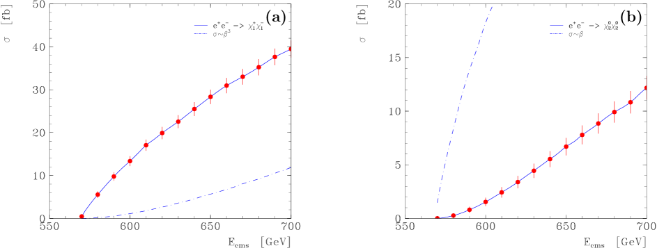
Figure 13: Cross sections of (a) $e^{+}e^{-}\to{\tilde{\chi}}^{+}_{1}{\tilde{\chi}}^{-}_{1}$ production and (b) $e^{+}e^{-}\to{\tilde{\chi}^{0}}_{2}{\tilde{\chi}^{0}}_{2}$ production close to threshold, including QED radiation, beamstrahlung and width effects. The statistical errors correspond to ${\cal L}=10\,\mathrm{fb}^{-1}$ per point, The dash-dotted curves indicate hypothetical cross section dependencies $\sigma_{{\tilde{\chi}}^{+}_{1}{\tilde{\chi}}^{-}_{1}}\sim\beta^{3}$ and $\sigma_{{\tilde{\chi}}^{0}_{2}{\tilde{\chi}}^{0}_{2}}\sim\beta$ for charginos and neutralinos, respectively.

The cross sections for ${\tilde{\chi}}^{+}_{1}{\tilde{\chi}}^{-}_{1}$ and ${\tilde{\chi}}^{0}_{2}{\tilde{\chi}}^{0}_{2}$ production as a function of energy are shown in Fig. 13(a) and Fig. 13(b), respectively. Since the masses are almost degenerate, the threshold energies of both reactions are very close and practically coincide. However, the chargino cross section rises much faster with $\sigma\sim\beta$ compared with the slow onset of the neutralino excitation curve $\sigma\sim\beta^{3}$. It is obvious from the threshold curves that the different (opposite) $\beta$ dependence for the two reactions can be easily ruled out.

As pointed out in the previous section, polarization effects in $\tilde{\chi}^{\pm}_{1}$ and $\tilde{\chi}^{0}_{2}$ decays must be exploited to determine the spin $J=1/2$ of the $\tilde{\chi}^{\pm}_{1}$ chargino and $\tilde{\chi}^{0}_{2}$ neutralino unambiguously.

(a) Charginos $\tilde{\chi}^{\pm}_{1}$:
The charginos in the production process $e^{+}e^{-}\to\tilde{\chi}^{-}_{1}\tilde{\chi}^{+}_{1}$ are polarized and even the polarization averaged over the production angle $\theta$ is in general non-zero (also for unpolarized beams). The cosine of the decay angle $\theta^{*}_{W^{\pm}}$ between the $W^{\pm}$ momentum direction in the chargino rest frame and the $\tilde{\chi}^{\pm}_{1}$ momentum direction in the laboratory frame, identical with the spin quantization axis, can be determined by measuring the $W^{\pm}$ energy in the hadronic $W^{\pm}$ decay $W^{\pm}\to q\bar{q}^{\prime}$:

$$E_{W^{\pm}}=\gamma\left(E^{*}_{W^{\pm}}+\beta\,p^{*}_{W^{\pm}}\cos\theta^{*}_{W^{\pm}}\right)$$ (4.44)

where $\gamma=\sqrt{s}/2m_{\tilde{\chi}^{\pm}_{1}}$ and $\beta=(1-4m^{2}_{\tilde{\chi}^{\pm}_{1}}/s)^{1/2}$. The $W^{\pm}$-boson energy and momentum in the chargino rest frame, $E^{*}_{W^{\pm}}$ and $p^{*}_{W^{\pm}}$, can be derived from the $\tilde{\chi}^{\pm}_{1},\tilde{\chi}^{0}_{1}$ and $W^{\pm}$ masses. Furthermore, the electric charge of the individual $W^{\pm}$ and $\tilde{\chi}^{\pm}_{1}$ can be identified by tagging the electric charge of the $W^{\mp}$ from the other chargino $\tilde{\chi}_{1}^{\mp}$ decay through the leptonic mode $W^{\mp}\to\ell^{\mp}\nu_{\ell}$. All these features can be used to study the $\tilde{\chi}^{\pm}_{1}$-polarization through the angular distribution in the two-body decays $\tilde{\chi}^{\pm}_{1}\to W^{\pm}\tilde{\chi}^{0}_{1}$. For the chargino as a spin-1/2 particle the decay distribution is linear in $\cos\theta^{*}_{W^{\pm}}$:

$$\frac{1}{d\Gamma}\frac{\Gamma}{d\cos\theta^{*}_{W^{\pm}}}\left[\tilde{\chi}^{\pm}_{1}\to W^{\pm}\tilde{\chi}^{0}_{1}\right]=\frac{1}{2}\left(1+\langle\kappa_{W^{\pm}}\rangle\cos\theta^{*}_{W^{\pm}}\right)$$ (4.45)

where the coefficient $\langle\kappa_{W^{\pm}}\rangle$ is the product of the $\tilde{\chi}^{\pm}_{1}$ polarization averaged over the production distribution and the $\tilde{\chi}^{\pm}_{1}$ polarization analysis power of the decay mode $\tilde{\chi}^{\pm}_{1}\to W^{\pm}\tilde{\chi}^{0}_{1}$; for details see Ref. [44]. The two coefficients $\langle\kappa_{W^{\pm}}\rangle$ are identical as a consequence of CP symmetry. The average helicities of $\tilde{\chi}^{-}_{1}$ and $\tilde{\chi}^{+}_{1}$ have the same magnitude but opposite sign in $e^{+}e^{-}$ annihilation for arbitrary beam polarization. For non-zero $\langle\kappa_{W^{\pm}}\rangle$ the decay angular distributions provide a unique signal for the spin $J=1/2$ of the chargino $\tilde{\chi}^{\pm}_{1}$.

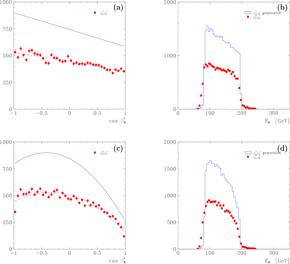
Figure 14: Chargino production $e^{+}e^{-}\to{\tilde{\chi}}^{+}_{1}{\tilde{\chi}}^{-}_{1}\to W^{+}{\tilde{\chi}^{0}}_{1}\;W^{-}{\tilde{\chi}^{0}}_{1}$ with $W^{\pm}$ decay angle distributions $\cos\theta^{*}_{W}$ in the ${\tilde{\chi}}^{\pm}_{1}$ rest frame (left panels) and $W^{\pm}$ energy distributions $E_{W}$ in the laboratory system (right panels). The plots (a) and (b) do not include QED radiation effects while the plots (c) and (d) include initial state photon radiation and beamstrahlung. Spectra at generator level (full curves and histograms) are compared with events simulated and reconstructed in the detector (dots), the dashed curves indicate fits to the data. The simulation is based on polarized beams with $({\cal P}_{e^{-}},{\cal P}_{e^{+}})=(-0.8,+0.6)$ at $\sqrt{s}=700\,\mathrm{GeV}$ and ${\cal L}=500\,\mathrm{fb}^{-1}$.

The $W^{\pm}$ decay angular distribution is studied in an experimental simulation of $e^{+}e^{-}\to{\tilde{\chi}}^{+}_{1}{\tilde{\chi}}^{-}_{1}$ production at $\sqrt{s}=700\,\mathrm{GeV}$, assuming the integrated luminosity of ${\cal L}=500\,\mathrm{fb}^{-1}$. With beam polarizations $({\cal P}_{e^{-}},{\cal P}_{e^{+}})=(-0.8,+0.6)$ the cross section amounts to $\sigma=150\,\mathrm{fb}$. The event signature is a reconstructed hadronic decay $W\to q\bar{q}^{\prime}$, a lepton from the decay $W\to\ell\nu$ ($\ell=e,\mu,\tau$) to select clean events, and large missing energy of $E^{\rm miss}>\sqrt{s}/2$. With a typical selection efficiency $\epsilon\simeq 0.6$ and a combined branching ratio ${\cal B}=0.44$ prolific event rates are expected. Background from other SM or SUSY processes is estimated to be small and will not be considered further. The chargino sample may be tripled by including events where both $W^{\prime}$s are allowed to decay to hadrons. However, the background will also increase due to false combinations of jets in reconstructing the two $W^{\prime}$s and due to background from ${\tilde{\chi}^{0}}_{2}{\tilde{\chi}^{0}}_{2}$ production (see above). Such a study goes beyond the aim of the present paper.

The basis of the analysis is Eq. (4.44) which relates the $W$ energy $E_{W}$ in the laboratory system with the decay angle $\cos\theta^{*}_{W^{\pm}}$ in the ${\tilde{\chi}}^{\pm}_{1}$ rest frame.

Figures 14(a) and (b) show the angular distribution and energy spectrum for the hypothetical case that no QED radiation degrades the nominal production energy. The linear $\cos\theta^{*}_{W^{\pm}}$ dependence is clearly seen at generator level as well as after detector simulation. A fit of the data to the function $d\sigma/d\cos\theta^{*}_{W^{\pm}}\sim 1+a^{0}_{1}\cos\theta^{*}_{W^{\pm}}+a^{0}_{2}\cos 2\theta^{*}_{W^{\pm}}$ yields $a^{0}_{1}=-0.213\pm 0.010$ and $a^{0}_{2}=-0.001\pm 0.010$. This value is consistent with the theoretical expectation of Eq. (4.45) with $\langle\kappa_{W^{\pm}}\rangle=-0.216$ and demonstrates that distortions due to event selection criteria and detector effects are small. The same tendency is observed in the energy distribution Fig. 14(b) which falls linearly with $E_{W}$, as compared with a flat distribution for unpolarized charginos.

In the more realistic situation that initial state photon radiation (ISR) and beamstrahlung decrease the ${\tilde{\chi}}^{+}_{1}{\tilde{\chi}}^{-}_{1}$ production energy, the angular distribution is no longer linearly falling, as shown in Fig. 14(c). Considerable depletions at $\cos\theta^{*}_{W^{\pm}}\to\pm 1$ are observed since the constraint $E_{{\tilde{\chi}}_{1}^{\pm}}$ is not always valid. However, since both ISR and beamstrahlung effects can be calculated theoretically and measured precisely, they can be unfolded from the data, e.g. by applying a bin-by-bin correction (like in the present analysis) or a matrix inversion procedure. Fitting of the QED corrected angular distribution (not shown) to the form

$$\frac{d\sigma^{\rm exp}}{d\cos\theta^{*}_{W^{\pm}}}\,\sim\,1+a_{1}\cos\theta^{*}_{W^{\pm}}+a_{2}\cos 2\theta^{*}_{W^{\pm}}$$ (4.46)

results in coefficients

$$a_{1}=-0.203\pm 0.020\quad\mbox{and}\quad a_{2}=-0.001\pm 0.020$$ (4.47)

These values are consistent with the input parameters and confirm with high precision the linear dependence on $\cos\theta^{*}_{W}$ characteristic for polarized spin 1/2 chargino production, while higher spin-$J$ states would generate the angular distribution

$$\frac{d\sigma}{d\cos\theta^{*}_{W^{\pm}}}\,\sim\,1+\sum^{2J}_{n=1}a_{n}\cos n\,\theta^{*}_{W^{\pm}}$$ (4.48)

A sensitivity of a few percents to any term in addition to the linear term can be reached which is an important bound in discriminating against higher spin $J>1/2$ states. Similar distortions due to QED radiation can be seen in the energy spectrum of Fig. 14(d) which is shifted towards lower values and is considerably depopulated at the maximum energy.

(b) Neutralino $\tilde{\chi}^{0}_{2}$:
The distribution of the polar angle in neutralino production $e^{+}e^{-}\to\tilde{\chi}^{0}_{2}\tilde{\chi}^{0}_{2}$ with two identical Majorana particles in the final state is forward-backward symmetric. The $\tilde{\chi}^{0}_{2}$ polarization, being non-zero for fixed polar angle, is asymmetric if the angle is varied from the forward to the backward direction [33]. The polarization degree can be enhanced by using polarized electrons/positrons beams.

The $\tilde{\chi}^{0}_{2}$ polarization can be determined [45] in the two-body decay $\tilde{\chi}^{0}_{2}\to Z\tilde{\chi}^{0}_{1}$ if the $Z$ polarization is measured in the leptonic decays $Z\to\ell^{+}\ell^{-}$. The measurement can also be performed for the hadronic decays $Z\to c\bar{c}$ and $b\bar{b}$ with $c$ and $b$ flavor tagging.

(Alternatively, if kinematically accessible,) the two-body leptonic decay $\tilde{\chi}^{0}_{2}\to\tilde{\ell}^{\pm}\ell^{\mp}$  can provide a powerful instrument for determining the $\tilde{\chi}^{0}_{2}$ spin. The $\tilde{\chi}^{0}_{2}$ momenta can be reconstructed, event by event, in $\tilde{\chi}^{0}_{2}$ pair production for sequential $\tilde{\chi}^{0}_{2}$ leptonic decays because the two unknown $\tilde{\chi}^{0}_{1}$ momenta can be fixed by measuring the four visible lepton momenta in the cascade decays $\tilde{\chi}^{0}_{2}\to\tilde{\ell}^{\pm}\ell^{\mp}\to\ell^{+}\ell^{-}\tilde{\chi}^{0}_{1}$ and $\tilde{\chi}^{0}_{2}\to\tilde{\ell^{\prime}}^{\pm}{\ell^{\prime}}^{\mp}\to{\ell^{\prime}}^{+}{\ell^{\prime}}^{-}\tilde{\chi}^{0}_{1}$. Furthermore, the slepton mode is a perfect polarization analyzer of the decaying neutralino. Explicitly, the angular distribution in the rest frame of the decaying spin-1/2 neutralino $\tilde{\chi}^{0}_{2}$ is given by [see Ref. [37]]

$$\frac{1}{\Gamma}\frac{\Gamma}{d\cos\theta^{*}_{\ell^{\mp}}}\left[\tilde{\chi}^{0}_{2}\to\tilde{\ell}^{\pm}_{R}\ell^{\mp}\right]=\frac{1}{2}\left(1\pm{\cal P}_{\tilde{\chi}^{0}_{2}}\cos\theta^{*}_{\ell^{\mp}}\right)$$ (4.49)

where ${\cal P}_{\tilde{\chi}^{0}_{2}}$ is the degree of longitudinal $\tilde{\chi}^{0}_{2}$ polarization and $\theta^{*}_{\ell^{\mp}}$ the angle of the $\ell^{\mp}$ momentum in the $\tilde{\chi}^{0}_{2}$ rest frame with respect to the $\tilde{\chi}^{0}_{2}$ momentum direction.

Therefore, the decays $\tilde{\chi}^{0}_{2}\to Z\tilde{\chi}^{0}_{1}$ and/or $\tilde{\chi}^{0}_{2}\to\tilde{\ell}\ell$ do provide a unique signal for the spin $J=1/2$ of the neutralino $\tilde{\chi}^{0}_{2}$.

Table 2: The threshold behavior and the angular distribution of SUSY and UED particle pair production, and the general characteristics of spin-$J$ field theories. All the characteristics refer to diagonal pair production. B and F_D,M generically denote bosons and Dirac, Majorana fermions; $[s]$ $s$-channel exchange only, $[s,t,u]$ potentially all three exchange mechanisms. The parameters $\kappa$ [$\kappa\neq-1$] depend on mass ratios and particle velocities $\beta$; note that, especially, $\kappa=1$ for Majorana fermions and for self-conjugate bosons [spin $\geq 1$] in $[s]$-channels – Notice the uniqueness of spin-0 assignments by measurements of the polar angle distribution in the slepton sector. Neither threshold excitation nor angular distributions are sufficient in the chargino/neutralino sector and final state analyses must be performed to determine the spin-1/2 quantum numbers.

Threshold Excitation and Angular Distribution
SUSY	particle	$\tilde{\mu}$	$\tilde{e}$	$\tilde{\chi}^{\pm}$	$\tilde{\chi}^{0}$
	spin	0	0	1/2	1/2
	$\sigma_{thr}$	$\beta^{3}$	$\beta^{3}$	$\beta$	$\beta^{3}$
	$\theta$ dep.	$\sin^{2}\theta$	thr: $\sin^{2}\theta$	thr: isotropic	thr: $1+\kappa\cos^{2}\theta$
UED	particle	$\mu_{1}$	$e_{1}$	$W^{\pm}_{1}$	$Z_{1}$
	spin	1/2	1/2	1	1
	$\sigma_{thr}$	$\beta$	$\beta$	$\beta$	$\beta$
	$\theta$ dep.	$1+\kappa^{2}\cos^{2}\theta$	thr: isotropic	thr: isotropic	thr: isotropic
General	particle	$B[s]$	$B[s,t,u]$	$F_{D,M}[s]$	$F_{D,M}[s,t,u]$
	spin	$\geq 1$	$\geq 1$	$\geq 1/2$	$\geq 1/2$
	$\sigma_{thr}$	$\beta^{3}$	$\beta$	$\beta,\beta^{3}$	$\beta,\beta^{3}$
	$\theta$ dep.	$1+\kappa\cos^{2}\theta$	thr: isotropic	$1+\kappa\cos^{2}\theta$	thr: $1+\kappa\cos^{2}\theta$

5 Summary

It is apparent from the preceding discussion that the model-independent determination of the spin quantum numbers of supersymmetric particles is a complex task, with the degree of complexity depending on the nature of the particle. Threshold excitation and angular distributions in pair production as well as angular correlations in particle decays provide the signals for experimental spin measurements.

The predictions for the threshold excitation and the angular distributions in the production processes of supersymmetric particles are summarized in Table 2. They are confronted with predictions for particles in models of universal extra space dimensions and with general analyses based on the non-vanishing of the magnetic dipole moments of all spin $>0$ particles.

Examining these results it turns out that the $\sin^{2}\theta$ law for the production of spin-0 sleptons [for selectrons close to threshold] is a unique signal of the spin-0 character. While the observation of the $\sin^{2}\theta$ angular distribution is sufficient for sleptons, the $\beta^{3}$ onset of the excitation curve is a necessary but not a sufficient condition for the spin-0 character. Thus the spin determination in the slepton sector is conceptually very simple at $e^{+}e^{-}$ colliders.

This simple pattern in the slepton sector must be contrasted with the more involved pattern in the spin-1/2 chargino/neutralino sector. Neither the onset of excitation curves nor the angular distributions in the production processes provide unique signals of the spin quantum numbers. However, decay angular distributions, $\sim|d^{J}(\theta^{\ast})|^{2}$, do provide a unique signal for the chargino/neutralino spin $J=1/2$, albeit at the expense of more involved experimental analyses. Using polarized electron/positron beams will in general assure that the decaying spin-1/2 particle is polarized; reasonable polarization analysis power is guaranteed in many decay processes.

In toto. The spin of sleptons and charginos/neutralinos can be determined in a model-independent way at $e^{+}e^{-}$ colliders. Similar methods as elaborated for sleptons can be applied in the squark sector while gluinos will demand a methodologically separate analysis.

Acknowledgments

The work was supported in part by the Korea Research Foundation Grant (KRF-2006-013-C00097), by KOSEF through CHEP at Kyungpook National University, by the Deutsche Forschungsgemeinschaft and by the Grant-in-Aid for Scientific Research (17540281 and 18340060) from MEXT, Japan. S.Y.C. thanks for support during his visit to DESY, while P.M.Z. gratefully acknowledges the warm hospitality extended to him by KEK.

Appendix: Cross sections with polarized beams

Polarized electron and positron beams at $e^{+}e^{-}$ colliders are useful for diagnosing the properties of supersymmetric particles and for unraveling the underlying structure of the SUSY theory [32]. In this Appendix we present the general formulae for the production cross sections of R-type smuon/electron pairs, and chargino and neutralino pairs in $e^{+}e^{-}$ annihilation with polarized electron and positron beams.

For longitudinal $e^{\pm}$ beam polarizations ${\cal P}_{e^{\pm}}$ the polarized production cross sections for R-type smuon and selectron pairs in $e^{+}e^{-}$ annihilation are given in terms of the charges $Q_{R}$ and $Q_{L}$ by

$$\frac{d\sigma}{d\cos\theta}\{\tilde{\ell}^{+}_{R}\tilde{\ell}^{-}_{R}\}\,=\,\frac{3}{32}\,\sigma_{0}\,\beta^{3}\sin^{2}\theta\,\bigg{[}(1-{\cal P}_{e^{-}}{\cal P}_{e^{+}})(|Q_{R}|^{2}+|Q_{L}|^{2})+({\cal P}_{e^{-}}-{\cal P}_{e^{+}})(|Q_{R}|^{2}-|Q_{L}|^{2})\bigg{]}$$ (A.1)

where $\tilde{\ell}_{R}=\tilde{\mu}_{R},\tilde{e}_{R}$ and $\sigma_{0}=4\pi\alpha^{2}/3s$ is the standard normalization cross section of $e^{+}e^{-}$ annihilation. The expressions of the generalized charges $Q_{R}$ and $Q_{L}$ for R-type smuon- and selectron-pair production can be found in Eqs. (2.3/2.2) and (3.4/3.3), respectively. For right/left polarized electrons ${\cal P}_{e^{-}}=\pm$ and unpolarized positrons, the production cross sections

$$\frac{d\sigma_{R}}{d\cos\theta}\{\tilde{\ell}^{+}_{R}\tilde{\ell}^{-}_{R}\}\,=\,\frac{3}{16}\,\sigma_{0}\,\beta^{3}\sin^{2}\theta\,|Q_{R}|^{2}$$ (A.2)

$$\frac{d\sigma_{L}}{d\cos\theta}\{\tilde{\ell}^{+}_{R}\tilde{\ell}^{-}_{R}\}\,=\,\frac{3}{16}\,\sigma_{0}\,\beta^{3}\sin^{2}\theta\,|Q_{L}|^{2}$$ (A.3)

project out the bilinear $R$ and $L$ charges $Q_{R}$ and $Q_{L}$.

The production cross sections for chargino- and neutralino-pairs in $e^{+}e^{-}$ annihilation with polarized electron and positron beams are given by

$$\mbox{ }\hskip-22.76228pt\frac{d\sigma}{d\cos\theta}\left\{\tilde{\chi}_{i}\tilde{\chi}_{j}\right\}\!\!\!\! = \!\!\!\frac{3}{8}\sigma_{0}\,\beta\,\bigg{[}(1-{\cal P}_{e^{-}}{\cal P}_{e^{+}})\left\{[1-(\mu^{2}_{i}-\mu^{2}_{j})^{2}+\beta^{2}\cos^{2}\theta]Q_{1}+4\mu_{i}\mu_{j}Q_{2}+2\beta\cos\theta Q_{3}\right\}$$ (A.4)

$${}\hskip 17.07182pt+({\cal P}_{e^{-}}-{\cal P}_{e^{+}})\left\{[1-(\mu^{2}_{i}-\mu^{2}_{j})^{2}+\beta^{2}\cos^{2}\theta]Q^{\prime}_{1}+4\mu_{i}\mu_{j}Q^{\prime}_{2}+2\beta\cos\theta Q^{\prime}_{3}\right\}\!\bigg{]}$$

where the $P$-even and $P$-odd quartic charges $Q_{i}$ and $Q^{\prime}_{i}$ ($i=1,2,3$) are defined in terms of the bilinear charges $Q_{\alpha\beta}$ ($\alpha,\beta=L,R$) as

$$Q^{(\prime)}_{1}\,=\,\frac{1}{4}\left[|Q_{RR}|^{2}+|Q_{RL}|^{2}\pm|Q_{LR}|^{2}\pm|Q_{LL}|^{2}\right]$$

$$Q^{(\prime)}_{2}\,=\,\frac{1}{2}\Re{\rm e}\left[Q_{RR}Q^{*}_{RL}\pm Q_{LL}Q^{*}_{LR}\right]$$

$$Q^{(\prime)}_{3}\,=\,\frac{1}{4}\left[|Q_{RR}|^{2}-|Q_{RL}|^{2}\pm|Q_{LR}|^{2}\mp|Q_{LL}|^{2}\right]$$ (A.5)

The explicit form of the bilinear charges $Q_{\alpha\beta}$ for the production of the chargino pair $\tilde{\chi}^{+}_{1}\tilde{\chi}^{-}_{1}$ and the neutralino pairs $\tilde{\chi}^{0}_{i}\tilde{\chi}^{0}_{j}$ is given in Eqs. (4.5) and (4.10), respectively. Polarized electrons combined with unpolarized positrons,

$$\frac{d\sigma_{R}}{d\cos\theta}\left\{\tilde{\chi}_{i}\tilde{\chi}_{j}\right\}\! = \!\frac{3}{16}\sigma_{0}\,\beta\,\bigg{[}\,[1-(\mu^{2}_{i}-\mu^{2}_{j})^{2}+\beta^{2}\cos^{2}\theta]\,(|Q_{RR}|^{2}+|Q_{RL}|^{2})$$ (A.6)

$${}\hskip 42.67912pt+8\mu_{i}\mu_{j}\,\Re{\rm e}(Q_{RR}Q^{*}_{RL})+2\beta\cos\theta(|Q_{RR}|^{2}-|Q_{RL}|^{2})\bigg{]}$$

$$\frac{d\sigma_{L}}{d\cos\theta}\left\{\tilde{\chi}_{i}\tilde{\chi}_{j}\right\}\! = \!\frac{3}{16}\sigma_{0}\,\beta\,\bigg{[}\,[1-(\mu^{2}_{i}-\mu^{2}_{j})^{2}+\beta^{2}\cos^{2}\theta]\,(|Q_{LR}|^{2}+|Q_{LL}|^{2})$$ (A.7)

$${}\hskip 42.67912pt+8\mu_{i}\mu_{j}\,\Re{\rm e}(Q_{LR}Q^{*}_{LL})+2\beta\cos\theta(|Q_{LR}|^{2}-|Q_{LL}|^{2})\bigg{]}$$

project out the bilinear charges $Q_{Rk}$ and $Q_{Lk}$ for the $\tilde{\chi}$ chirality $k=R,L$.

References

• [1] J. Wess and B. Zumino, Nucl. Phys. B 70 (1974) 39; J. Wess and B. Zumino, Phys. Lett. B 49 (1974) 52.
• [2] H. P. Nilles, Phys. Rept. 110 (1984) 1; H. E. Haber and G. L. Kane, Phys. Rept. 117 (1985) 75; D. J. H. Chung, L. L. Everett, G. L. Kane, S. F. King, J. Lykken and L. -T. Wang, Phys. Rept. 407 (2005) 1.
• [3] T. Appelquist, H. C. Cheng and B. A. Dobrescu, Phys. Rev. D 64 (2001) 035002 [arXiv:hep-ph/0012100].
• [4] H. C. Cheng, K. T. Matchev and M. Schmaltz, Phys. Rev. D 66 (2002) 036005 [arXiv:hep-ph/0204342].
• [5] W. Beenakker, R. Hopker, M. Spira and P. M. Zerwas, Nucl. Phys. B 492 (1997) 51 [arXiv:hep-ph/9610490].
• [6] G. Weiglein et al. [LHC/LC Study Group], Phys. Rept. 426 (2006) 47 [arXiv:hep-ph/0410364].
• [7] A. Datta, K. Kong and K. T. Matchev, Phys. Rev. D 72, 096006 (2005) [Erratum-ibid. D 72, 119901 (2005)] [arXiv:hep-ph/0509246].
• [8] A. J. Barr, Phys. Lett. B 596, 205 (2004) [arXiv:hep-ph/0405052]; JHEP 0602, 042 (2006) [arXiv:hep-ph/0511115]; J. M. Smillie and B. R. Webber, JHEP 0510 (2005) 069 [arXiv:hep-ph/0507170]; C. Athanasiou, C. G. Lester, J. M. Smillie and B. R. Webber, JHEP 0608 (2006) 055 [arXiv:hep-ph/0605286].
• [9] S.Y. Choi, K. Hagiwara, Y.G. Kim, K. Mawatari and P.M. Zerwas, arXiv:hep-ph/0612237.
• [10] D. J. Miller, S. Y. Choi, B. Eberle, M. M. Muhlleitner and P. M. Zerwas, Phys. Lett. B 505 (2001) 149.
• [11] M. T. Dova, P. Garcia-Abia and W. Lohmann, LC-PHSM-2001-055.
• [12] H.-U. Martyn, LC-PHSM-2003-07, arXiv:hep-ph/0302024; see also Ref. [14].
• [13] M. Battaglia, A. Datta, A. De Roeck, K. Kong and K. T. Matchev, JHEP 0507, 033 (2005) [arXiv:hep-ph/0502041].
• [14] E. Accomando et al. [ECFA/DESY LC Physics Working Group], Phys. Rept.  299 (1998) 1 [arXiv:hep-ph/9705442]; J. A. Aguilar-Saavedra et al. [ECFA/DESY LC Physics Working Group], “TESLA Technical Design Report Part III: Physics at an e+e- Linear Collider”, edited by R.-D. Heuer, D. Miller, F. Richard and P. M. Zerwas, arXiv:hep-ph/0106315; T. Abe et al. [American Linear Collider Working Group], “Linear collider physics resource book for Snowmass 2001. 4: Theoretical, in Proc. of the APS/DPF/DPB Summer Study on the Future of Particle Physics (Snowmass 2001) ed. N. Graf, arXiv:hep-ex/0106058; K. Abe et al. [ACFA Linear Collider Working Group], arXiv:hep-ph/0109166; W. Kilian and P. M. Zerwas, arXiv:hep-ph/0601217.
• [15] E. Accomando et al. [CLIC Physics Working Group], arXiv:hep-ph/0412251.
• [16] A. Freitas, D. J. Miller and P. M. Zerwas, Eur. Phys. J. C 21, 361 (2001) [arXiv:hep-ph/0106198].
• [17] A. Freitas, A. von Manteuffel and P. M. Zerwas, Eur. Phys. J. C 34, 487 (2004) [arXiv:hep-ph/0310182]; Eur. Phys. J. C 40, 435 (2005) [arXiv:hep-ph/0408341].
• [18] J. A. Aguilar-Saavedra et al., Eur. Phys. J. C 46 (2006) 43 [arXiv:hep-ph/0511344].
• [19] S. Ferrara, M. Porrati and V. L. Telegdi, Phys. Rev. D 46, 3529 (1992).
• [20] S. U. Chung, Phys. Rev. D 57 (1998) 431; S. Z. Huang, T. N. Ruan, N. Wu and Z. P. Zheng, Eur. Phys. J. C 26 (2003) 609.
• [21] M. Nowakowski, E. A. Paschos and J. M. Rodriguez, Eur. J. Phys.  26 (2005) 545 [arXiv:physics/0402058].
• [22] L. P. S. Singh and C. R. Hagen, Phys. Rev. D 9 (1974) 898. L. P. S. Singh and C. R. Hagen, Phys. Rev. D 9 (1974) 910.
• [23] F. E. Paige, S. D. Protopopescu, H. Baer and X. Tata, arXiv:hep-ph/0312045.
• [24] T. Sjöstrand, P. Edén, C. Friberg, L. Lönnblad, G. Miu, S. Mrenna and E. Norrbin, Comput. Phys. Commun.  135 (2001) 238 [arXiv:hep-ph/0010017].
• [25] T. Ohl, Comput. Phys. Commun.  101 (1997) 269 [arXiv:hep-ph/9607454].
• [26] Tesla Technical Design Report, DESY 2001-011, “TESLA Technical Design Report Part IV: A Detector for TESLA”, edited by T. Behnke, S. Bertolucci, R.-D. Heuer, R. Settles.
• [27] M. Pohl and H. J. Schreiber, DESY-02-061, arXiv:hep-ex/0206009.
• [28] H.-U. Martyn and G. A. Blair, arXiv:hep-ph/9910416; H.-U. Martyn, arXiv:hep-ph/0406123.
• [29] S. T. Boogert and D. J. Miller, arXiv:hep-ex/0211021, and refrences quoted therein.
• [30] H.-U. Martyn, arXiv:hep-ph/0002290.
• [31] A. Freitas, H. U. Martyn, U. Nauenberg and P. M. Zerwas, arXiv:hep-ph/0409129.
• [32] G. Moortgat-Pick et al., arXiv:hep-ph/0507011.
• [33] S. Y. Choi, J. Kalinowski, G. Moortgat-Pick and P. M. Zerwas, Eur. Phys. J. C 22, 563 (2001) [Addendum-ibid. C 23, 769 (2002)] [arXiv:hep-ph/0108117].
• [34] L. M. Sehgal and P. M. Zerwas, Nucl. Phys. B 183, 417 (1981).
• [35] B. C. Allanach et al., in Proc. of the APS/DPF/DPB Summer Study on the Future of Particle Physics (Snowmass 2001) ed. N. Graf, Eur. Phys. J. C 25 (2002) 113 [eConf C010630 (2001) P125] [arXiv:hep-ph/0202233].
• [36] N. Ghodbane and H.-U. Martyn, in Proc. of the APS/DPF/DPB Summer Study on the Future of Particle Physics (Snowmass 2001) ed. N. Graf, arXiv:hep-ph/0201233.
• [37] S. Y. Choi, M. Drees and J. Song, JHEP 0609, 064 (2006) [arXiv:hep-ph/0602131].
• [38] S. Y. Choi, A. Djouadi, M. Guchait, J. Kalinowski, H. S. Song and P. M. Zerwas, Eur. Phys. J. C 14, 535 (2000) [arXiv:hep-ph/0002033]; S. Y. Choi, M. Guchait, J. Kalinowski and P. M. Zerwas, Phys. Lett. B 479, 235 (2000) [arXiv:hep-ph/0001175].
• [39] F. Boudjema and C. Hamzaoui, Phys. Rev. D 43 (1991) 3748.
• [40] S. Y. Choi, Phys. Rev. D 69 (2004) 096003 [arXiv:hep-ph/0308060].
• [41] W. Alles, C. Boyer and A. J. Buras, Nucl. Phys. B 119 (1977) 125.
• [42] K. Hagiwara, R. D. Peccei, D. Zeppenfeld and K. Hikasa, Nucl. Phys. B 282 (1987) 253.
• [43] Large Detector Concept working group, http://ilcdc.org.
• [44] S. Y. Choi, A. Djouadi, H. K. Dreiner, J. Kalinowski and P. M. Zerwas, Eur. Phys. J. C 7 (1999) 123 [arXiv:hep-ph/9806279].
• [45] A. Bartl, H. Fraas, O. Kittel and W. Majerotto, Eur. Phys. J. C 36 (2004) 233 [arXiv:hep-ph/0402016].