1-3 leptonic mixing and the neutrino oscillograms of the Earth

Abstract:

We develop a detailed and comprehensive description of neutrino oscillations driven by the 1-3 mixing in the matter of the Earth. The description is valid for the realistic (PREM) Earth density profile in the whole range of nadir angles and for neutrino energies above 1 GeV. It can be applied to oscillations of atmospheric and accelerator neutrinos. The results are presented in the form of neutrino oscillograms of the Earth, i.e. the contours of equal oscillation probabilities in the neutrino energy–nadir angle plane. A detailed physics interpretation of the oscillograms, which includes the MSW peaks, parametric ridges, local maxima, zeros and saddle points, is given in terms of the amplitude and phase conditions. Precise analytic formulas for the probabilities are obtained. We study the dependence of the oscillation pattern on $\theta_{13}$ and find, in particular, that the transition probability $P>1/2$ appears for $\sin^{2}2\theta_{13}$ as small as $\sim 0.009$. We consider the dependence of the oscillation pattern on the matter density profile and comment on the possibility of the oscillation tomography of the Earth.

1 Introduction

Substantial future progress in neutrino physics will be related to the long baseline experiments as well as studies of the cosmic and atmospheric neutrinos. The key element of these experiments is that neutrinos propagate long distances inside the Earth before reaching detectors. Oscillations in the matter of the Earth change flavor properties of neutrino fluxes, which opens up possibilities to

• study dynamics of various oscillation effects;

• determine yet unknown oscillation parameters: 1-3 mixing, deviation of the 2-3 mixing from maximal and its octant, the type of the neutrino mass hierarchy, and CP-violation;

• perform the oscillation tomography of the Earth;

• search for various new effects caused by non-standard neutrino interactions and/or by exotic physics (such as violation of Lorentz or CPT invariance).

The sensitivity of present-day experiments to the corresponding effects, that appear usually as small corrections to the leading oscillation phenomena (e.g. $\nu_{\mu}\leftrightarrow\nu_{\tau}$ vacuum oscillations), is rather low. In the case of atmospheric neutrinos this is related to low fluxes and therefore low statistics of events, and also to uncertainties in the fluxes. The accelerator neutrino beams are, in principle, well controlled, however in majority of the projects the baselines are relatively short, whereas the very long baseline experiments (e.g. with neutrino factories) employ high energy neutrinos. This means that the region of energy $E_{\nu}\sim(3-10)$ GeV and nadir angle $\Theta_{\nu}=0-70^{\circ}$, where the most interesting oscillation phenomena occur, is not covered. Therefore one needs to rely on high precision measurements of the suppressed “tails” of these phenomena. The dilemma is whether to study small effects with a number of systematical errors and degeneracies, or develop experimental approaches that will allow to cover the regions of large oscillation effects. The latter option is realized in the concepts of very long baseline accelerator experiments and very large volume atmospheric neutrino detectors.

In connection with possible future experimental developments and discussions of new strategies of research, a detailed and comprehensive study of physics of the neutrino oscillations in the Earth is needed. Some studies in this direction have been carried out in the past.

In the matter of the Earth, the resonance enhancement of $\nu_{e}\leftrightarrow\nu_{\mu}$ and $\nu_{\tau}$ oscillations can take place [1, 2], with the MSW resonance peak at $E_{\nu}/\Delta m^{2}\sim 2.5\times 10^{3}~{}\text{GeV}/\text{eV}^{2}$ [3, 4]. It was also recognized that the size of the Earth is comparable with the neutrino refraction length, and consequently strong enhancement of oscillations can occur for rather deep trajectories (small nadir angles) and not too small mixing angles: $\sin^{2}2\theta_{13}>0.03$. With decreasing baseline, first the matter effect and then the oscillation effect disappear. This phenomenon  [1, 5], termed “vacuum mimicking”, implies that for short baselines the flavour transitions are described by the vacuum oscillation formula.

For 1-2 mixing the resonance is in the neutrino channel and at rather low energies: $E_{\nu}\sim 0.1$ GeV. For non-zero 1-3 mixing the MSW resonance peak related to the atmospheric mass splitting is at $E_{\nu}\sim 6$ GeV. The peak is narrow and, depending on the mass hierarchy, the enhancement occurs in the neutrino (normal hierarchy) or antineutrino (inverted hierarchy) channels. Possibilities to observe this resonance peak have been explored in connection to the measurements of the mixing angle $\theta_{13}$ and determination of the neutrino mass hierarchy [6, 7, 8, 9, 10, 11, 12]. Furthermore, it was realized that matter effects can also strongly influence $\nu_{\mu}\leftrightarrow\nu_{\tau}$ oscillations [13, 14].

A qualitatively new oscillation phenomenon can be realized for neutrinos crossing the core of the Earth due to a sharp change of the density at the border between the core and the mantle [15, 16, 17, 18, 19, 20]. In particular, for non-zero 1-3 mixing, the existence of an additional peak is predicted in the energy distribution between the peaks due to the MSW resonances in the core and mantle. This core-mantle effect was interpreted as being due to the parametric enhancement of neutrino oscillations [15, 17, 18]. The additional peak is a manifestation of the parametric resonance for 3 layers (1.5 period of the “castle wall” profile) in matter [21]. The parametric resonance occurs when the variation of the matter density along the neutrino trajectory is in a certain way correlated with the values of the oscillation parameters [22, 23, 24]. A different interpretation of this peak, as being due to an interference between the contributions to the oscillation amplitude from different layers of the Earth’s mantle and core, has been discussed in [16, 19, 20]. It was uncovered [25] that the parametric resonance condition is fulfilled also at large energies (above the mantle MSW resonance), leading to the appearance of two parametric peaks in the nadir angle distribution. For general consideration of evolution in the multi-layer media, see [26].

Apart from the large scale structures of the density profile, effects of small scale density perturbation have been explored [27].

Analytic approaches have been developed to describe the physics of various oscillation effects, to understand the influence of the density profile modifications on the oscillation probabilities and also to simplify numerical computations. Many studies have been performed in the constant density approximation [3, 4] or approximation of several layers of constant densities [15, 16, 17, 18, 19, 20, 23, 24, 28, 13, 29]. For the varying densities within the layers a perturbation-theory approach has been developed in [30] for the description of the solar neutrino oscillations in the Earth.

For $3\nu$ mixing the analytic approaches employ various expansions in the small parameters $\sin^{2}\theta_{13}$ and/or in the ratio of the mass squared differences $\Delta m^{2}_{21}/\Delta m^{2}_{31}$ [31]. For the case of non-constant density matter, different perturbation theory approaches have been developed for oscillations in low density [32, 33] and high density [34, 25] media. In [25] an analytic description of oscillations in the high energy limit has been worked out for the case of the realistic (PREM) density profile. The influence of the Earth density profile on the oscillation probabilities has also been considered in [35].

To some extent, the results obtained so far had fragmentary character. This paper is the first one in a series of papers we devote to a detailed and comprehensive study of oscillations of neutrinos inside the Earth. Here we present a thorough description of neutrino oscillations caused by non-zero 1-3 mixing, with the emphasis on the physics of the phenomenon. In particular, we study the complex pattern and interplay of various oscillation resonances. We show that the main features of this complex pattern can be easily understood in terms of different realizations of just two simple conditions – the amplitude condition and the phase condition. We perform our study in terms of “neutrino oscillograms” of the Earth: contours of constant oscillation probabilities in the plane of neutrino energy and nadir angle. These plots have been presented in several earlier publications as illustrations [19, 8, 36]. Here we use them as the main tool of the study. We present a description of all the structures of the oscillograms and of their dependence on $\theta_{13}$ and the density profile. We generalize the amplitude and the phase conditions to the case of non-constant densities in the layers of matter and develop an appropriate analytic formalism.

The paper is organized as follows. In Sec. 2, after some generalities, we introduce the neutrino oscillograms of the Earth, concentrating mainly on $\nu_{e}\leftrightarrow\nu_{\mu}(\nu_{\tau})$ transitions. We discuss the accuracy of the constant-density layers approximation of the Earth matter profile and describe the graphical representation of the conversion. In Sec. 3 we give the physics interpretation of the oscillograms. In Sec. 4 we derive approximate analytic formulas for probabilities for a realistic matter density profile. In Sec. 5 we study the dependence of the oscillograms on the 1-3 mixing and the density profile of the Earth, and we discuss the oscillation probabilities for the other channels. Discussion and conclusions follow in Sec. 6.

2 Neutrino oscillograms of the Earth

2.1 Context. Evolution matrix

We consider the three-flavor neutrino system with the state vector $\nu_{f}\equiv(\nu_{e},\,\nu_{\mu},\,\nu_{\tau})^{T}$. Its evolution in matter is described by the equation

$$i\frac{d\nu_{f}}{dx}=\left(\frac{UM^{2}U^{\dagger}}{2E_{\nu}}+\hat{V}(x)\right)\nu_{f}\,,$$ (1)

where $E_{\nu}$ is the neutrino energy and $M^{2}\equiv\mathop{\mathrm{diag}}(0,\,\Delta m^{2}_{21},\,\Delta m^{2}_{31})$ is the diagonal matrix of neutrino mass squared differences. $\hat{V}(x)\equiv\mathop{\mathrm{diag}}(V(x),\,0,\,0)$ is the matrix of matter-induced neutrino potentials with $V(x)\equiv\sqrt{2}G_{F}N_{e}(x)$, $G_{F}$ and $N_{e}(x)$ being the Fermi constant and the electron number density, respectively. The mixing matrix $U$ defined through $\nu_{f}=U\nu_{m}$, where $\nu_{m}=(\nu_{1},\,\nu_{2},\,\nu_{3})^{T}$ is the vector of neutrino mass eigenstates, can be parameterized as

$$U=U_{23}I_{\delta}U_{13}I_{-\delta}U_{12}\,.$$ (2)

Here the matrices $U_{ij}=U_{ij}(\theta_{ij})$ describe rotations in the $ij$-planes by the angles $\theta_{ij}$, and $I_{\delta}\equiv\mathop{\mathrm{diag}}(1,\,1,\,e^{i\delta})$, where $\delta$ is the Dirac-type CP-violating phase.

Let us introduce the evolution matrix (the matrix of transition and survival amplitudes) $S(x,x_{0})$, which describes the evolution of the neutrino state over a finite distance: from $x_{0}$ to $x$. To simplify the presentation, throughout the paper we will use the notation $S(x)\equiv S(x,0)$ and $S\equiv S(L)$, where $L$ is the total length of the trajectory. The matrix $S(x)$ satisfies the same evolution equation as the state vector (1):

$$i\frac{dS(x)}{dx}=H(x)\,S(x)\,.$$ (3)

The solution of equation (3) with the initial condition $S(0)=\mathbbm{1}$ can be formally written as

$$S(x)=T\exp\left(-i\int_{0}^{x}H\,dx\right)\,.$$ (4)

It is convenient to consider the evolution of the neutrino system in the propagation basis, $\tilde{\nu}=(\nu_{e},\,\tilde{\nu}_{2},\,\tilde{\nu}_{3})^{T}$, defined through the relation

$$\nu_{f}=U_{23}I_{\delta}\tilde{\nu}\,.$$ (5)

As follows from (1) and (2), the Hamiltonian $\tilde{H}$, that describes the evolution of the neutrino vector of state $\tilde{\nu}$, is

$$\tilde{H}(x)=\frac{1}{2E_{\nu}}U_{13}U_{12}M^{2}U^{\dagger}_{12}U^{\dagger}_{13}+\hat{V}(x)\,.$$ (6)

This Hamiltonian does not depend on the 2-3 mixing and CP-violating phase. The dependence on these parameters appears when one projects the initial state on the propagation basis and the final state back onto the original flavor basis. Explicitly, the Hamiltonian $\tilde{H}$ reads

$$\tilde{H}(x)=\frac{\Delta m^{2}_{31}}{2E_{\nu}}\begin{pmatrix}s_{13}^{2}+s_{12}^{2}\,c_{13}^{2}\,r_{\Delta}+2V(x)E_{\nu}/\Delta m^{2}_{31}&s_{12}\,c_{12}\,c_{13}\,r_{\Delta}&s_{13}\,c_{13}(1-s^{2}_{12}\,r_{\Delta})\\ \ldots&c_{12}^{2}\,r_{\Delta}&-s_{12}\,c_{12}\,s_{13}\,r_{\Delta}\\ \ldots&\ldots&c_{13}^{2}+s_{12}^{2}\,s_{13}^{2}\,r_{\Delta}\end{pmatrix}$$ (7)

where $c_{ij}\equiv\cos\theta_{ij}$, $s_{ij}\equiv\sin\theta_{ij}$ and

$$r_{\Delta}\equiv\frac{\Delta m^{2}_{21}}{\Delta m^{2}_{31}}\,.$$ (8)

According to (5), the evolution matrix $\tilde{S}(x)$ in the basis $(\nu_{e},\tilde{\nu}_{2},\tilde{\nu}_{3})$ is related to $S(x)$ by the transformation:

$$S(x)=\tilde{U}\,\tilde{S}(x)\,\tilde{U}^{\dagger},\qquad\tilde{U}\equiv U_{23}I_{\delta}.$$ (9)

The evolution of $\tilde{S}(x)$ is given by the equation analogous to Eq. (3) with the Hamiltonian $\tilde{H}(x)$.

2.2 High energy neutrino approximation

For sufficiently high energies ($E_{\nu}>1-2$ GeV) one can neglect the 1-2 mass splitting. Then, according to (7), the state $\tilde{\nu}_{2}$ decouples from the rest of the system and does not evolve. Therefore, if we parameterize $\tilde{S}$ in the basis $(\nu_{e},\tilde{\nu}_{2},\tilde{\nu}_{3})$ as

$$\tilde{S}=\begin{pmatrix}A_{ee}&A_{e2}&A_{e3}\\ A_{2e}&A_{22}&A_{23}\\ A_{3e}&A_{32}&A_{33}\end{pmatrix}$$ (10)

we find that in this approximation $A_{e2}=A_{2e}=A_{23}=A_{32}=0$, $A_{22}=1$ and the evolution matrix in the flavor basis takes the form

$$S\approx\begin{pmatrix}A_{ee}&s_{23}A_{e3}&c_{23}A_{e3}\\ s_{23}A_{3e}&c_{23}^{2}A_{22}+s_{23}^{2}A_{33}&-s_{23}c_{23}(A_{22}-A_{33})\\ c_{23}A_{3e}&-s_{23}c_{23}(A_{22}-A_{33})&s_{23}^{2}A_{22}+c_{23}^{2}A_{33}\end{pmatrix}\,,$$ (11)

where we omitted the CP-phase factor $e^{-i\delta}$ since CP-violating effects are absent in the limit $r_{\Delta}\to 0$. We will consider the complete $3\nu$ system in the next publication [37]. Denoting

$$P_{A}\equiv|A_{e3}|^{2}=|A_{3e}|^{2}\,,$$ (12)

we obtain from (11)

$$P(\nu_{e}\to\nu_{e}) =1-P_{A},$$ (13)

$$P(\nu_{e}\to\nu_{\mu}) =P(\nu_{\mu}\to\nu_{e})=s_{23}^{2}P_{A}\,,$$ (14)

$$P(\nu_{e}\to\nu_{\tau}) =P(\nu_{\tau}\to\nu_{e})=c_{23}^{2}P_{A}\,,$$ (15)

$$P(\nu_{\mu}\to\nu_{\mu}) =1-s_{23}^{4}P_{A}-2s_{23}^{2}c_{23}^{2}\,\left[1-\mathop{\mathrm{Re}}A_{33}\right]\,,$$ (16)

$$P(\nu_{\mu}\to\nu_{\tau}) =-s_{23}^{2}\,c_{23}^{2}\,P_{A}+2s_{23}^{2}c_{23}^{2}\,\left[1-\mathop{\mathrm{Re}}A_{33}\right]\,.$$ (17)

The formulas in Eqs. (13–17) reproduce the probabilities derived in [18].

Thus, in the approximation $\Delta m^{2}_{21}=0$ the dynamical problem is reduced to two flavor evolution problem. Throughout this paper we work in the basis where, for a 2-flavor neutrino system, $H_{11}=-H_{22}=-\cos 2\theta_{13}\Delta m^{2}/4E+V/2$. This can be always achieved by subtracting from $H$ a matrix proportional to the unit matrix and correspondingly rephasing the neutrino vector of state. This symmetric Hamiltonian is related to the Hamiltonian of the 1-3 subsystem $\tilde{H}^{(13)}$, obtained from Eq. (7) by taking the limit $r_{\Delta}=0$ and removing the decoupled state $\tilde{\nu}_{2}$, as

$$\tilde{H}^{(13)}=H+\left(\frac{\Delta m^{2}}{4E_{\nu}}+\frac{V}{2}\right)\mathbbm{1}\,.$$ (18)

For the $2\nu$ case the unitary evolution matrix can be parameterized as

$$S=\begin{pmatrix}\hphantom{-}\alpha&\beta\\ -\beta^{*}&\alpha^{*}\end{pmatrix}\,,\qquad|\alpha|^{2}+|\beta|^{2}=1.$$ (19)

For density profiles that are symmetric with respect to the midpoint of the neutrino trajectory (for brevity, symmetric profiles), T invariance leads to the equality of the off-diagonal elements of the evolution matrix, $\beta=-\beta^{*}$, which means that $\beta$ is pure imaginary [38].

For a single layer of constant density the solution can be written explicitly:

$$S(x)=\begin{pmatrix}\cos\phi(x)+i\cos 2\theta_{m}\,\sin\phi(x)&-i\sin 2\theta_{m}\,\sin\phi(x)\\ -i\sin 2\theta_{m}\,\sin\phi(x)&\cos\phi(x)-i\cos 2\theta_{m}\,\sin\phi(x)\end{pmatrix},\quad\phi(x)\equiv\bar{\omega}\,x\,.$$ (20)

Here is $\theta_{m}$ is the mixing angle in matter and $\phi(x)$ is the half-phase of oscillations in matter with

$$\bar{\omega}=\omega(\bar{V})\equiv\sqrt{\left(\cos 2\theta_{13}\frac{\Delta m^{2}_{31}}{4E_{\nu}}-\frac{\bar{V}}{2}\right)^{2}+\left(\sin 2\theta_{13}\frac{\Delta m^{2}_{31}}{4E_{\nu}}\right)^{2}}.$$ (21)

The moduli squared of the elements of ${S}$ reproduce the well-known probabilities for oscillations in a uniform medium. Thus in the notation of Eq. (19),

$$\alpha=\cos\phi+i\cos 2\theta_{m}\,\sin\phi\,,\qquad\beta=-i\sin 2\theta_{m}\,\sin\phi\,.$$ (22)

In what follows we will generalize this result to the cases of several layers of constant densities and also of changing densities within the layers.

The scale of the matter effects in neutrino oscillations is set up by the refraction length, $l_{0}\equiv 2\pi/(\sqrt{2}G_{F}N_{e})$, which is comparable with the radius of the Earth $R=6371$ km. The oscillation length in matter $l_{m}$ is given by

$$\frac{2\pi}{l_{m}}=2\bar{\omega}\,.$$ (23)

At high energies the length $l_{m}$ essentially coincides with the refraction length: $l_{m}\simeq l_{0}$. In the resonance channel, with decreasing energy $l_{m}$ increases and reaches its maximum slightly above the resonance energy. At the MSW resonance, $E_{\nu}=E_{R}$, one has $l_{m}=l_{\nu}/\sin 2\theta_{13}$, where $l_{\nu}$ is the vacuum oscillation length. Below the resonance, with energy further decreasing, $l_{m}$ decreases and approaches $l_{\nu}$: $l_{m}(E_{\nu}\ll E_{R})\approx l_{\nu}$.

In a non-uniform density medium the adiabatic half-phase of oscillations is defined as

$$\phi(x)\equiv\int_{0}^{x}\omega(x^{\prime})\,dx^{\prime}\,,\qquad\omega(x)\equiv\omega(V(x))\,.$$ (24)

2.3 Neutrino oscillograms of the Earth

For given values of $|\Delta m^{2}_{31}|$, $\sin^{2}2\theta_{13}$, and the type of neutrino mass hierarchy, the oscillation probabilities depend on the neutrino energy $E_{\nu}$ and the nadir angle of its trajectory $\Theta_{\nu}$. Therefore a complete description of the oscillation pattern can be given by contours of equal oscillation probabilities in the $(E_{\nu},\,\Theta_{\nu})$ plane. We call the resulting figures the neutrino oscillograms of the Earth. The plots of this type were produced for the first time by P. Lipari in 1998 (unpublished) and then appeared in several later publications [19, 8, 36]. Here we will employ this kind of plots as the main tool of our study.

We use in our calculations the matter density distribution inside the Earth, $\rho$, as given by the PREM model [39]. It exhibits a characteristic structure with a relatively slow density change within the mantle and within the core and a sudden jump of density by about a factor of two at their border. Smaller jumps appear between the inner core and the outer one and near the surface of the Earth. The number of electrons per nucleon, $Y_{e}\equiv N_{e}m_{N}/\rho$ where $m_{N}$ is the nucleon mass, equals $Y_{e}=0.497$ in the mantle and $Y_{e}=0.468$ in the core. For the energies $E_{\nu}>(1-2)$ GeV the oscillation length in vacuum $l_{\nu}$ exceeds 1000 km, and therefore the effects of smaller-scale density perturbations are averaged out. Furthermore, the density profile experienced by neutrinos along any trajectory inside the Earth is symmetric with respect to the midpoint of the trajectory, so that

$$V(x)=V(L-x),$$ (25)

where $L=2R\cos\Theta_{\nu}$ is the length of the trajectory. As we will see below, to a large extent this feature determines the properties of the oscillation probabilities and the structure of the oscillograms.

For numerical calculations we use the current best-fit value of $\Delta m^{2}_{31}=2.5\times 10^{-3}$ eV; in the case of negligible effects of 1-2 splitting, changing $\Delta m^{2}_{31}$ is equivalent to correspondingly rescaling the neutrino energy.

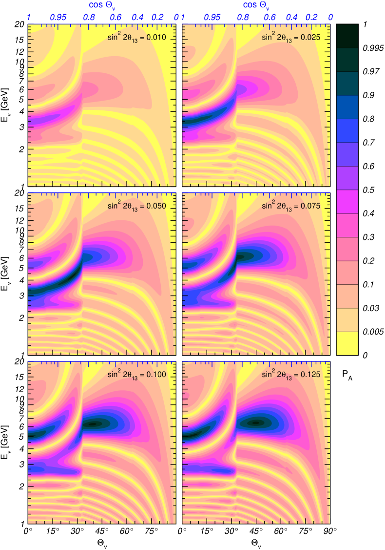
Figure 1: Neutrino oscillograms of the Earth. Shown are the contours of constant probability $P_{A}$ (edges of the shadowed regions) in the plane of the nadir angle of the neutrino trajectory $\Theta_{\nu}$ and neutrino energy $E_{\nu}$, for different values of the mixing angle $\theta_{13}$.

In Fig. 1 we present the oscillograms for the transition probability $P_{A}$ for normal mass hierarchy and several values of $\sin^{2}2\theta_{13}$. The oscillograms have two regions, separated by $\Theta_{\nu}=33.1^{\circ}$ that corresponds to the nadir angle of the border between the core and the mantle. For $\Theta_{\nu}<33.1^{\circ}$, the neutrino trajectories cross the core of the Earth, so that neutrinos traverse two mantle layers and one core layer. For brevity we call this part the core domain of the oscillogram. Conversely, the region $\Theta_{\nu}>33.1^{\circ}$ corresponds to the mantle-only crossing trajectories, and we call it the mantle domain. As follows from the figure, there are several salient, generic features of the oscillation picture:

• the MSW resonance pattern (resonance enhancement of the oscillations) for mantle-only crossing trajectories, with the main peak at $E_{\nu}\sim(5-7)$ GeV;

• three parametric resonance ridges in the core domain, at $E_{\nu}>3$ GeV;

• the MSW resonance pattern in the core domain, $E_{\nu}<3$ GeV, with the core resonance ridge at $E_{\nu}=2.5-2.7$ GeV;

• regular oscillatory pattern for low energies: valleys of zero probability and ridges in the mantle domain and more complicated pattern with local maxima and saddle points in the core domain.

The small windings of the contours at $\Theta_{\nu}=65^{\circ}$ and $70^{\circ}$ correspond to the borders of the transition zone between the inner and upper mantle, while the windings at $\Theta_{\nu}=11^{\circ}$ are due to the border between the inner and outer core. In what follows we will show that the whole this, apparently complicated, picture can be understood in terms of different realizations of just two conditions: the amplitude condition and the phase condition.

2.4 Constant-density layers approximations

As we shall see, the main features of the oscillograms can be well understood using the approximation of constant-density layers for the density distribution inside the Earth. Furthermore, this consideration allows us to evaluate the sensitivity of the oscillograms to changes of the profile. In Figs. 2 and 3 we show the oscillograms computed for two different approximations of this kind:

• Approximation of fixed constant-density layers, when the Earth density profile is described by the core and mantle layers of constant densities that are the same for all neutrino trajectories. This approximation has been widely used in the literature. For definiteness, we have taken $\rho_{1}=5.5$ g/cm³ and $\rho_{2}=11.5$ g/cm³, which roughly correspond to the average densities in the core and in the mantle. In Fig. 2 we compare the $P_{A}$-oscillograms calculated in this approximation and the exact results. The approximation reproduces the oscillation pattern qualitatively well, with all the features present. However, quantitatively its accuracy is not high above $E_{\nu}>3$ GeV, in particular, in the resonance region, and for deep trajectories $\Theta_{\nu}<60^{\circ}$. For instance, one can observe an upward shift of the approximate contours compared to the exact ones by about 1 GeV at $E_{\nu}\simeq(6-10)$ GeV. The shift decreases with increasing $\Theta_{\nu}$.

• Approximation of the path-dependent (trajectory-dependent) constant density layers. For each trajectory we find the average potentials $\bar{V}_{1}$ and $\bar{V}_{2}$ in the mantle and in the core, respectively,

  $$\bar{V}_{i}(\Theta_{\nu})=\frac{1}{L_{i}(\Theta_{\nu})}\int_{0}^{L_{i}}V_{i}(x)\,dx\,,\qquad i=1,2,$$ (26)

  where $L_{i}(\Theta_{\nu})$ is the trajectory length in the $i$-th layer, and then use the oscillation probability formulas for one or three layers of constant densities. In Fig. 3 we show the $P_{A}$ oscillograms calculated in this approximation. One can see that the accuracy of the approximation is noticeably better than that of the fixed-density approximation, especially for the core-crossing trajectories. Again, the largest difference appears for the deep mantle trajectories and $E_{\nu}>5$ GeV.

As can be seen from Figs. 2 and 3, the accuracy of the constant-density layers approximations improves with decreasing neutrino energy, the reason being that the matter effects become less important for small $E_{\nu}$. These approximations also in general work better for the core-crossing trajectories because they are dominated by the evolution in the core and because inside the core the density changes only by about 30%, whereas in the mantle it changes by about a factor of two. For mantle-only crossing trajectories, the approximations work better for shorter trajectories, closer to the surface. Here again the matter effects becomes weaker due to the vacuum mimicking phenomenon [1, 5].

Thus, the approximations of constant-density layers reproduce correctly the qualitative structure of the oscillograms obtained with the realistic PREM density profile of the Earth. All the resonance peaks, ridges and other structures present for the PREM-profile appear also in the approximate profile calculations, though their location and shape is not always well reproduced. Therefore one can use these approximations for understanding the main qualitative features of the results for realistic profiles.

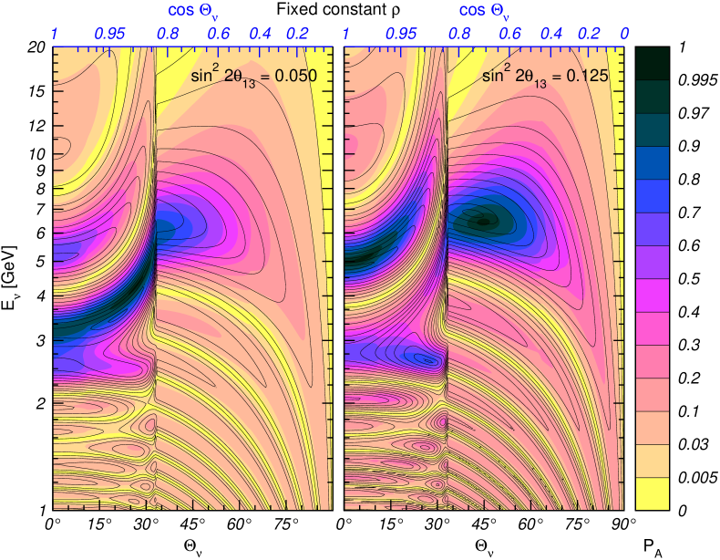
Figure 2: The $P_{A}$ oscillograms for the PREM density profile (colored regions; grayscale on black-and-white printouts) and for the fixed constant-density layers approximation (black curves).

Figure 3: The $P_{A}$ oscillograms for the PREM density profile (colored regions; grayscale on black-and-white printouts) and for the path-dependent constant-density layers approximation (black curves).

2.5 Graphical representation

For illustrative purposes we will also use the graphical representation of the $2\nu$ oscillations based on their analogy with spin precession in a magnetic field [3, 40]. Let us introduce the neutrino “spin” vector in the flavor space $\vec{s}=\{s_{X},\,s_{Y},\,s_{Z}\}$ with the components

$$s_{X}(x)=\mathop{\mathrm{Re}}[S_{11}^{*}(x)\,S_{12}(x)]\,,\quad s_{Y}(x)=\mathop{\mathrm{Im}}[S_{11}^{*}(x)\,S_{12}(x)]\,,\quad s_{Z}(x)=|S_{11}(x)|^{2}-\frac{1}{2}\,.$$ (27)

These components are essentially the elements of the density matrix. The evolution equation for the vector $\vec{s}(x)$ can be obtained from the evolution equation for $S(x)$, given in Eq. (3):

$$\frac{d\vec{s}}{dx}=2\,\vec{B}(x)\times\vec{s}(x)\,,$$ (28)

where

$$\vec{B}(x)=\vec{B}(V(x))=\frac{\Delta m^{2}}{4E_{\nu}}\left\{\sin 2\theta,\;0,\;\frac{2E_{\nu}V(x)}{\Delta m^{2}}-\cos 2\theta\right\}\,.$$ (29)

In this representation the oscillations in a medium with constant density is equivalent to a precession of the vector $\vec{s}$ on the surface of the cone (which we will call the precession cone) with the axis $\vec{B}(\bar{V})$ and the opening angle $2\theta_{m}$. According to Eq. (29) the axis of the cone is located in the $(X,\,Z)$ plane and the angle between the cone axis and the $Z$ axis equals $2\theta_{m}$. In a medium with non-constant density profile the cone axis turns following the change of the angle $2\theta_{m}(V(x))$. The opening angle of the cone does not change in the adiabatic case, and it changes if the adiabaticity is broken.

3 Physics interpretation of the oscillograms

In this section we give a physics interpretation and description of the four main structures of the oscillograms mentioned in Sec. 2.3, as well as of the contours of zero probability.

3.1 Resonance enhancement of oscillations in the mantle

The oscillation pattern in the mantle is determined by the resonance enhancement of the oscillations [1, 2]. In the constant-density approximation, for a given $\Theta_{\nu}$ the probability $P_{A}$ is an oscillatory function of energy, which is inscribed in the resonance curve $\sin^{2}2\theta_{m}(E_{\nu})$. The position of the maximum of the resonance peak is given by the MSW resonance condition:

$$E_{\nu}=E_{R}(\Theta_{\nu})=\frac{\Delta m^{2}_{31}\cos 2\theta_{13}}{2\bar{V}_{1}(\Theta_{\nu})}\,,$$ (30)

where $\bar{V}_{1}(\Theta_{\nu})$ is the average value of the potential along the trajectory characterized by $\Theta_{\nu}$ (see Eq. (26)). Eq. (30) determines the resonance line in the $(E_{\nu},\,\Theta_{\nu})$ plane. With the increase of $\Theta_{\nu}$ the average potential decreases and consequently $E_{R}$ increases. According to Fig. 1, for the MSW resonance in the mantle we have $E_{R}\sim 6$ GeV. The resonance width $\Delta E_{\nu}/E_{R}\sim 2\tan 2\theta_{13}$. The condition $E_{\nu}=E_{R}(\Theta_{\nu})$ ensures that the amplitude of oscillations is maximal and we will call it the amplitude (or resonance) condition.

Another condition that should be met to obtain the absolute maximum of the transition probability, $P_{A}=1$, is the phase condition:

$$2\phi(E_{\nu},\Theta_{\nu})=2\omega(\bar{V},E_{\nu})L(\Theta_{\nu})=(2k+1)\pi$$ (31)

which means that the oscillation phase should be an odd integer of $\pi$. Since the size of the Earth is comparable with the refraction length in the mantle $l_{0}=2\pi/\bar{V}$, the condition of the absolute maximum (31) can only be fulfilled for $k=0$, i.e. when the length of the neutrino trajectory coincides with the half of the oscillation length in matter. The phase condition (31) gives another curve in the $(E_{\nu},\,\Theta_{\nu})$ plane. The intersection of the resonance line (30) and the phase condition line (31) gives the absolute maximum of $P_{A}$. Combining (30) and (31) we conclude that the absolute maximum corresponds to the situation when for the resonance energy the oscillation phase is $\pi$:

$$2\omega(\bar{V},E_{R})L(\Theta_{\nu})=\pi\,.$$ (32)

Since $L=2R\cos\Theta_{\nu}$ and at the resonance $2\omega=\sin 2\theta_{13}(\Delta m^{2}_{31}/2E_{\nu})$, the phase condition (32) yields

$$\cos\Theta_{\nu}=\frac{\pi E_{\nu}}{R\sin 2\theta_{13}\Delta m^{2}_{31}}\,.$$ (33)

With the increase of $\theta_{13}$ the peak shifts to smaller values of $\cos\Theta_{\nu}$ (see Fig. 1).

Let us now reformulate the resonance and the phase conditions for the case of varying density within the mantle. For this we first express these conditions in terms of the elements of the evolution matrix using the explicit results for matter of constant density, Eqs. (19) and (20), and then use the obtained conditions also in the case of varying matter density.

As concerns to the resonance condition, $\cos 2\theta_{m}=0$, it can be written according to Eqs. (19) and (22) as $\alpha=\alpha^{*}$, i.e.

$$S_{11}^{(1)}=S_{22}^{(1)}\,,$$ (34)

or equivalently,

$$\mathop{\mathrm{Im}}S_{11}^{(1)}=0\,,$$ (35)

where the superscript indicates the number of layers. This generalization, however, goes beyond the original MSW-resonance condition. For the constant density case it gives

$$\cos 2\theta_{m}\sin\phi=0\,.$$ (36)

This condition has two realizations: the original one

$$\cos 2\theta_{m}=0\,,$$ (37)

and

$$\phi=\pi k,\qquad(k=1,2,\ldots)$$ (38)

and the latter corresponds to $P_{A}=0$, which is realized at low energies. In the case of varying density (e.g., in the mantle of the Earth), there is no factorization of the resonance condition (35) into path-dependent and path-independent factors, as in Eq. (36). However, when the density varies slowly enough along the neutrino path, in certain limits Eq. (35) is still approximately realized in the form of Eqs. (37) or (38). At low energies the MSW resonance condition is not fulfilled in the Earth’s mantle, and therefore the only possible realization of (35) is the one in Eq. (38). In contrast to this, for large energies and small distances Eq. (38) is not satisfied, and the only way Eq. (35) can be implemented is through the MSW resonance (37). In the intermediate region neither of the two conditions (37) and (38) is satisfied. Thus, in the resonance region Eq. (35) interpolates between the MSW resonance condition and the condition $\phi=\pi$.

As for the phase condition, $\phi=\pi/2+\pi k$, again we can rewrite it in terms of the elements of the evolution matrix, and from Eqs. (19) and (22) we get

$$\mathop{\mathrm{Re}}\alpha\equiv\mathop{\mathrm{Re}}S_{11}^{(1)}=0\,.$$ (39)

The absolute maximum of the transition probability occurs when both conditions (35) and (39) are satisfied simultaneously. In this case $S_{11}^{(1)}=0$ and $P_{A}=1$. This situation corresponds to $\phi=\pi/2$, and from Fig. 1 we see that it is realized only for $\sin^{2}2\theta_{13}\gtrsim 0.08$.

3.2 Parametric ridges and generalized resonance condition

For core-crossing trajectories and $E_{\nu}>3$ GeV the oscillatory picture is characterized by three ridges of enhanced oscillation probability. The ridges are the curves along which the probability decreases most slowly from its local or absolute maximum. The lower-energy ridge, which we will call the ridge “$A$”, corresponds to the energies in between those of the MSW resonances in the core and in the mantle, $E_{\nu}>(3-6)$ GeV. It was interpreted in [15, 17, 18] as being due to the parametric enhancement of neutrino oscillations. The other two ridges, “$B$” and “$C$”, extend above the MSW resonance energy in the mantle. They were also identified as the effects of the parametric enhancement of neutrino oscillations [25]. Here we shall further elaborate on this interpretation.

Recall that the parametric resonance occurs in oscillating systems with varying parameters when the rate of the parameter change is in a special correlation with the values of the parameters themselves. Neutrino oscillations in matter can undergo parametric enhancement if the length and size of the density modulation are correlated in a certain way with neutrino parameters [22, 23]. This enhancement is completely different from the MSW effect; in particular, no level crossing is required.

An example admitting exact analytic solution, and in fact, relevant for our discussion, is the “castle wall” density profile [23, 17]. This is a periodic step function with one period consisting of two layers of widths $L_{1}$ and $L_{2}$ and electron number densities $N_{1}$ and $N_{2}$. For 2-flavor neutrino oscillations, the evolution matrix over one period of density modulation can be written as

$$S^{(2)}=Y\mathbbm{1}-i{\boldsymbol{\sigma}}\cdot\mathbf{X}\,,$$ (40)

where $Y$ and $\mathbf{X}=(X_{1},\,X_{2},\,X_{3})$ are real parameters satisfying $Y^{2}+\mathbf{X}^{2}=1$ and $\sigma_{i}$ are the Pauli matrices in the flavor space. The oscillation probability for an arbitrary number of layers traversed by neutrinos can be written as a product of the amplitude

$$A=\frac{X_{1}^{2}+X_{2}^{2}}{X_{1}^{2}+X_{2}^{2}+X_{3}^{2}}\,,$$ (41)

which does not depend on the number of the layers, and an oscillating factor, which depends on this number [17]. The amplitude $A$ reaches its maximum when $X_{3}=0$, or explicitly [17]

$$X_{3}=-(s_{1}c_{2}\cos 2\theta_{1}+s_{2}c_{1}\cos 2\theta_{2})=0,$$ (42)

where $s_{1,2}\equiv\sin\phi_{1,2}$ and $c_{1,2}\equiv\cos\phi_{1,2}$. Here $2\phi_{1,2}$ are the oscillation phases acquired in the layers $1$ and $2$, and $\theta_{1,2}$ are the corresponding mixing angles in matter. Note that in the constant-density limit ($N_{1}=N_{2}$ or $\theta_{1}=\theta_{2}=\theta_{m}$) this condition reduces to Eq. (36) with $\phi=\phi_{1}+\phi_{2}$. For $\sin\phi\neq 1$ it coincides with the MSW resonance condition, which is the maximum amplitude condition for oscillations in a matter of constant density.

As was pointed out above, the Earth density profile seen by neutrinos with core-crossing trajectories can be very well approximated by three layers of constant densities, which is nothing but a piece of the castle wall profile; the layers “1” and “2” have to be identified with the Earth’s mantle and core, respectively. It has been demonstrated that the parametric resonance condition (42) can be satisfied for oscillations of core-crossing neutrinos for a rather wide range of nadir angles both at intermediate energies [15, 16, 17] and high energies [25], leading to significant enhancement of the oscillation probability. Thus, despite the fact that the Earth’s density profile consists of only three layers, the effects can be quite substantial. This show the relevance of the parametric resonance interpretation of this phenomenon, even for just “1.5 periods” of density modulation [21].

The parametric resonance condition (42) can be readily generalized to the case of non-constant densities in the mantle and the core of the Earth, though the generalization is not unique. Indeed, according to (40) the condition $X_{3}=0$ can be written in terms of elements of the evolution matrix for two layers as the equality of the diagonal elements:

$$S_{11}^{(2)}=S_{22}^{(2)}.$$ (43)

We will use this equality for an arbitrary density distribution within the layers and call it the generalized resonance condition. Note that parameterization (40) of the matrix $S^{(2)}$ implies that the generalized resonance condition can also be formulated as the requirement that the diagonal element of $S^{(2)}$ be real: $\mathop{\mathrm{Im}}S_{11}^{(2)}=0$.

In the right panels of Fig. 4 we show the curves of the generalized parametric resonance condition. Apparently, all the three parametric ridges are very well described by these curves.

Since condition (42) does not depend on the number of layers traversed by neutrinos, it only ensures that the parametric oscillations occur with the maximal depth, that is, after some number of periods of density modulation $P\approx 1$. In general, the condition of maximal transition probability for a given number of layers need not coincide with the condition of maximal amplitude of the parametric oscillations. Thus, the fact that Eq. (42) and the generalized condition (43) give the correct description of ridges for the Earth density profile with three layers is rather non-trivial.

3.3 Parametric effects and collinearity condition

Another approach to the generalization of the parametric resonance condition to the case of the layers of non-constant density is based on the consideration of the evolution amplitudes in the individual layers. For the particular case of two layers of constant densities, similar considerations have been presented in [20].

For density profiles consisting of two layers we have

$$S^{(2)}=S_{2}\,S_{1}=\begin{pmatrix}S_{11}^{(2)}&S_{12}^{(2)}\\ -S_{12}^{(2)*}&S_{11}^{(2)*}\end{pmatrix}\,,$$ (44)

where

$$S_{11}^{(2)}=\alpha_{2}\,\alpha_{1}-\beta_{2}\,\beta_{1}^{*}\,,\qquad S_{12}^{(2)}=\alpha_{2}\,\beta_{1}+\beta_{2}\,\alpha_{1}^{*}\,,$$ (45)

and $\alpha_{i}$, $\beta_{i}$ for each layer have been defined in Eq. (22). The sum of the two complex numbers in the transition amplitude $S_{12}^{(2)}$ can potentially lead to the largest possible result (if they add in the same phase and not in the anti-phase) if the two contributions to $S_{12}$ have the same complex phase (modulo $\pi$):

$$\arg(\alpha_{2}\beta_{1})=\arg(\beta_{2}\alpha_{1}^{*})\quad\mbox{mod}(\pi)\,.$$ (46)

It can also be rewritten as

$$\arg(\alpha_{1}\alpha_{2}\beta_{1})=\arg(\beta_{2})\quad\mbox{mod}(\pi)\,.$$ (47)

We shall call this condition the collinearity condition. It is an extremality condition for the two-layer transition probability under the constraint of fixed transition probabilities in the individual layers. In other words, if the absolute values $|\beta_{i}|$ of the transition amplitudes are fixed while their arguments are allowed to vary, the transition probability reaches an extremum when these arguments satisfy (46) or (47). For a realistic situation (neutrino oscillations in the Earth), changes of $E_{\nu}$ and $\Theta_{\nu}$ produce correlated changes of the arguments and the absolute values of the individual amplitudes, and therefore in general the condition (46) may not correspond to extrema precisely.

If the layers 1 and 2 have constant densities, then $\alpha_{i}=c_{i}+i\cos 2\theta_{i}\,s_{i}$, $\beta_{i}=-i\sin 2\theta_{i}\,s_{i}\,$ (see (22)), and the condition in Eq. (46) reproduces the parametric resonance condition (42), i.e. $X_{3}=0$. Under this condition the diagonal elements of $S^{(2)}$ are real; therefore, in the case of constant-density layers the collinearity condition, the generalized resonance condition and the parametric resonance condition coincide.

Denoting by $\chi_{\alpha i}$ and $\chi_{\beta i}$ the arguments of the complex amplitudes $\alpha_{i}$ and $\beta_{i}$, respectively, one can rewrite the collinearity condition as

$$\chi_{\alpha 1}+\chi_{\alpha 2}=\chi_{\beta 2}-\chi_{\beta 1}\quad\mbox{mod}(\pi)\,.$$ (48)

Consider now the case of three layers of in general varying densities. For the elements of the evolution matrix $S^{(3)}$ one obtains

$$S_{11}^{(3)} =\alpha_{3}\,S_{11}^{(2)}-\beta_{3}\,S_{12}^{(2)*}=\alpha_{3}\,\alpha_{2}\,\alpha_{1}-\alpha_{3}\,\beta_{2}\,\beta_{1}^{*}-\beta_{3}\,\alpha_{2}^{*}\,\beta_{1}^{*}-\beta_{3}\,\beta_{2}^{*}\,\alpha_{1}\,,$$ (49)

$$S_{12}^{(3)} =\alpha_{3}\,S_{12}^{(2)}+\beta_{3}\,S_{11}^{(2)*}=\alpha_{3}\,\alpha_{2}\,\beta_{1}+\alpha_{3}\,\beta_{2}\,\alpha_{1}^{*}+\beta_{3}\,\alpha_{2}^{*}\,\alpha_{1}^{*}-\beta_{3}\,\beta_{2}^{*}\,\beta_{1}\,.$$ (50)

In the case of neutrino oscillations in the Earth, the third layer is just the second mantle layer, and its density profile is the reverse of that of the first layer. The evolution matrix for the third layer is therefore the transpose of that for the first one [38], i.e. $\alpha_{3}=\alpha_{1}$, $\beta_{3}=-\beta_{1}^{*}$, and the expression for $S_{12}^{(3)}$ can be written as

$$S_{12}^{(3)}=\alpha_{1}\alpha_{2}\beta_{1}-\alpha_{1}^{*}\alpha_{2}^{*}\beta_{1}^{*}+|\alpha_{1}|^{2}\beta_{2}+|\beta_{1}|^{2}\beta_{2}^{*}\,.$$ (51)

Note that $\beta_{2}$ is pure imaginary because the core density profile is symmetric. Therefore the amplitude $S_{12}^{(3)}$ in Eq. (51) is also pure imaginary, as it must be because the overall density profile of the Earth is symmetric as well. It is easy to see that if the collinearity condition for two layers (47) is satisfied, then not only the full amplitude $S_{12}^{(3)}$, but also each of the four terms on the right hand side of Eq. (51) is pure imaginary. We therefore conclude that if the collinearity condition is satisfied for two layers, then it is automatically satisfied for three layers as well. It should be stressed that this is a consequence of the facts that the density profile of the third layer is the reverse of that of the first layer and that the second layer has a symmetric profile. Once again, the collinearity of all the contributions to the transition amplitude potentially leads to the maximal total transition probability for given transition probabilities in each layer.

Let us now confront the generalized resonance condition and the collinearity condition. For two layers the generalized resonance condition can be written as

$$-X_{3}=\mathop{\mathrm{Im}}S_{11}^{(2)}=\mathop{\mathrm{Im}}(\alpha_{2}\alpha_{1}-\beta_{2}\beta^{*}_{1})=0$$ (52)

or, in terms of the moduli and complex phases of the amplitudes,

$$|\alpha_{2}\alpha_{1}|\sin(\chi_{\alpha 1}+\chi_{\alpha 2})=|\beta_{2}\beta_{1}|\sin(\chi_{\beta 2}-\chi_{\beta 1})\,.$$ (53)

Comparing (53) and (48) we come to the following conclusions:

• If the generalized resonance condition (53) has to be satisfied independently of the moduli, then $\chi_{\alpha 1}+\chi_{\alpha 2}=\chi_{\beta 1}-\chi_{\beta 2}=\pi k$, and the collinearity condition (48) is satisfied too.

• If the collinearity condition is fulfilled, then the generalized resonance condition (53) can be rewritten as

  $$\sin(\chi_{\beta 1}-\chi_{\beta 2})\left[|\alpha_{2}\alpha_{1}|\pm|\beta_{1}\beta_{2}|\right]=0\,,$$ (54)

  which is satisfied provided that

  $$\chi_{\beta 1}=\chi_{\beta 2}\quad\mbox{mod}(\pi)\,.$$ (55)

  This condition is, in particular, fulfilled when the density profiles in both layers are symmetric (e.g., in the constant-density layers case), since in that case $\chi_{\beta 1}=\chi_{\beta 2}=\pm\pi/2$ as a consequence of T-invariance.

Thus, we conclude that for symmetric profiles in each of the two layers (and, in particular, for constant-density layers) the generalized resonance condition and the collinearity condition coincide. For layers of non-symmetric densities, the two conditions differ. As can be seen in the right panels of Fig. 4, both conditions describe the parametric enhancement ridges in the oscillograms quite well. This is a consequence of the fact that the matter density profiles felt by neutrinos traversing the Earth can be well approximated by path-dependent constant density layers.

3.4 Extrema and saddle points

As has been discussed above, in the constant density case the positions of maxima of the oscillation probability are determined by two conditions: the amplitude condition and the phase condition.

For matter of non-constant density, the collinearity condition or the 2-layer generalized resonance condition can be considered as the generalizations of the amplitude condition. Taking into account that the density profile of the Earth’s core is symmetric (i.e. $\mathop{\mathrm{Re}}\beta_{2}=0$), one can rewrite the collinearity condition (47) as

$$\mathop{\mathrm{Re}}(\alpha_{1}\alpha_{2}\beta_{1})=0\,.$$ (56)

Compared with Eq. (47), this condition has the practical advantage of not being trivially satisfied for $\beta_{2}=0$, which has no physically relevant implications. For trajectories crossing only the mantle of the Earth, one has to set $\alpha_{2}=1$ in Eq. (56) and the collinearity condition reduces to $\mathop{\mathrm{Re}}(\alpha_{1}\beta_{1})=0$. Recall that in the limit of constant matter density in the mantle this latter condition reduces to the condition of maximal mixing in matter (barring $\phi_{1}=\pi k$).

The phase condition $\phi=\pi/2+\pi k$ of the constant-density case can be generalized for varying density by expressing it in terms of the elements of the evolution matrix. According to (22), for one layer and the phase $\phi=\pi/2+\pi k$ the product of amplitudes $\alpha\beta^{*}=\pm\sin 2\theta\cos 2\theta$ is real. Therefore, we can generalize the phase condition $\mathop{\mathrm{Im}}(\alpha\beta^{*})$ taking instead of $\alpha$ and $\beta$ the elements of the evolution matrix (amplitudes) for an arbitrary profile:

$$\mathop{\mathrm{Im}}(S_{11}S_{12}^{*})=0.$$ (57)

Furthermore, since for symmetric density profiles $S_{12}$ is pure imaginary, Eq. (57) gives

$$\mathop{\mathrm{Re}}S_{11}=0\,,$$ (58)

i.e., the phase condition is fulfilled when $S_{11}$ is pure imaginary.

In the graphical representation of neutrino oscillations based on their analogy with spin precession in a magnetic field (see Sec. 3.6), Eq. (57) corresponds to the condition that the neutrino “spin” vector is in the $(s_{X},\,s_{Z})$ plane. As can be easily seen, this is equivalent to the requirement that the transition probability be stationary with respect to small variations of the total distance $L$ traveled by neutrinos: $dP_{A}/dL=0$.

In the right panels of Fig. 4 we plot the collinearity (amplitude) condition, the generalized resonance condition and the phase condition for two different values of $\sin^{2}2\theta_{13}$.

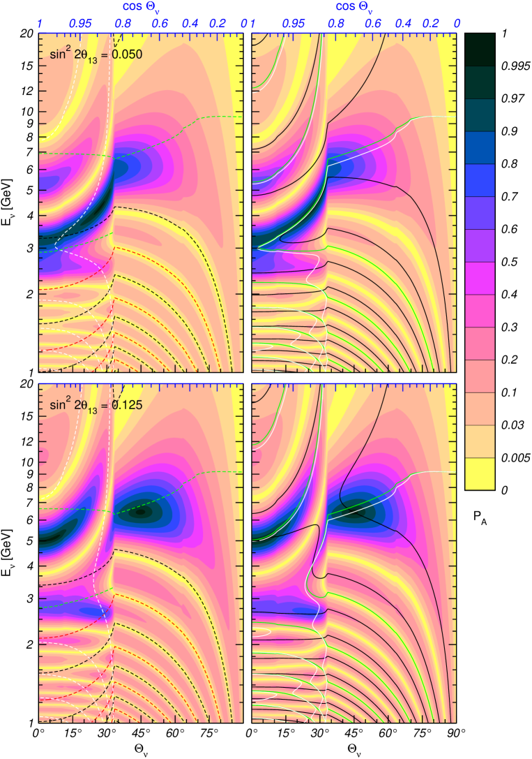
Figure 4: $P_{A}$ oscillograms and curves of phase and amplitude conditions for the PREM profile. Left panels: the MSW resonance (dashed green), $\mathop{\mathrm{Re}}\alpha_{1}=0$ (dashed black), $\mathop{\mathrm{Im}}\beta_{1}=0$ (dashed red) and $\mathop{\mathrm{Re}}\alpha_{2}=0$ (dashed white). Right panels: collinearity condition (solid white), generalized resonance condition (solid green) and phase condition (solid black).

As follows from the figure, the simultaneous fulfillment of the phase and amplitude conditions leads not only to absolute maxima of the transition probability ($P_{A}=1$), as in the constant density case, but also to local maxima and saddle points. This is an effect of the multi-layer medium. To figure out why this happens, we will use the explicit results for three layers of constant densities. In this case [17]

$$S_{11}^{(3)}=Z-iW_{3}\,,$$ (59)

where

$$Z=2c_{1}Y-c_{2}\,,\qquad W_{3}=-(2s_{1}Y\cos 2\theta_{1}+s_{2}\cos 2\theta_{2})\,,$$ (60)

and

$$Y=c_{1}c_{2}-s_{1}s_{2}\cos 2(\theta_{1}-\theta_{2})\,.$$ (61)

Both $Z$ and $W_{3}$ are real and therefore the phase condition (58) gives $Z=0$, i.e.:

$$2c_{1}Y-c_{2}=0\qquad\text{(phase condition)}.$$ (62)

Also in this case

$$P_{A}=1-W_{3}^{2}.$$ (63)

The collinearity condition (56) reduces to $\sin 2\theta_{1}s_{1}X_{3}=0\,$ for constant density layers, and since $\sin 2\theta_{1}\neq 0$, we have

$$s_{1}X_{3}=0\qquad\text{(amplitude condition)}.$$ (64)

Let us analyze possible realizations of these two conditions. According to (62), there are two ways to satisfy the phase condition: (i) $c_{1}\neq 0$, $Y=c_{2}/2c_{1}$ and (ii) $c_{1}=0$, $c_{2}=0$. The amplitude condition (64) also has two realizations: (i) $X_{3}=0$, ($s_{1}\neq 0$), and (ii) $s_{1}=0$, ($X_{3}\neq 0$). As we will see below, different consistent combinations of these realizations lead to absolute maxima, local maxima or saddle points of $P_{A}$.

In the non-constant density case, we will use Eq. (56) as the general amplitude condition and Eq. (58) as the general phase condition. Using Eq. (22), we generalize the other equalities discussed above as

$$c_{1}=0~{} \rightarrow~{}\mathop{\mathrm{Re}}\alpha_{1}=0,$$ (65)

$$c_{2}=0~{} \rightarrow~{}\mathop{\mathrm{Re}}\alpha_{2}=0,$$ (66)

$$s_{1}=0~{} \rightarrow~{}\mathop{\mathrm{Im}}\beta_{1}=0.$$ (67)

In the left panels of Fig. 4 we show the curves that correspond to different conditions. From the constant-density limit it is clear why the curves $\mathop{\mathrm{Im}}\beta_{1}=0$ always coincide with some of the amplitude condition curves: this follows from the fact that $\mathop{\mathrm{Im}}\beta_{1}=0$ is a particular solution of the amplitude condition.

Let us now consider all consistent realizations of the amplitude and phase conditions, using the terminology of the constant density approximation:

$\bullet$ $X_{3}=0$ ($s_{1}\neq 0$) (amplitude); $Y=c_{2}/2c_{1}$ ($c_{1}\neq 0$) (phase). Plugging this expression for the phase condition in (60), we obtain

$$W_{3}=\frac{X_{3}}{c_{1}}\,.$$ (68)

Since $X_{3}=0$ by the amplitude condition, we have $W_{3}=0$ and, consequently, from Eq. (63) $P_{A}=1$. Thus, in the constant density layers approximation a simultaneous fulfillment of the phase and collinearity conditions should lead to $P_{A}=1$, provided that $c_{1}\neq 0$ or $\pm 1$. This possibility is realized only on the ridge $A$, at a point where the two curves that correspond to the generalized amplitude and phase conditions cross. The other curves, depicting the conditions (65), (66) and (67), cannot pass through this point. Notice that at this crossing point the oscillation half-phases in the core and mantle differ from $\pi/2$ and $\pi$, and there is a nontrivial interplay between the phases and mixing angles in the parametric resonance condition (42).

$\bullet$ $c_{1}=0$, $c_{2}=0$ (the latter equality follows from Eq. (62)) (the phase condition). In this case the amplitude condition, $X_{3}=0$, is satisfied automatically. Using the explicit formulas for $Y$ (61), $W_{3}$ (60) and Eq. (63), we obtain $Y=\pm\cos 2(\theta_{1}-2\theta_{2})$ and

$$P_{A}=\sin^{2}(4\theta_{1}-2\theta_{2})\,.$$ (69)

This case corresponds to the core and mantle half-phases equal to $\pi/2+\pi k$. It has a simple graphical representation, when it is enough to consider neutrino “spin” vector in the $(X,\,Z)$ plane (see Sec. 3.6 below). This representation immediately leads to the expression in Eq. (69) for the transition probability [15], and shows that this probability has a maximum for neutrino energies between those of the core and mantle MSW resonances (where $\cos 2\theta_{1}>0$ and $\cos 2\theta_{2}<0$), provided that $(\theta_{2}-\theta_{1})>\pi/4$, and above the MSW resonances, where $\cos 2\theta_{1,2}<0$. Below the resonances and between the resonances for $(\theta_{2}-\theta_{1})$ $\leq\pi/4$, Eq. (69) corresponds to a saddle point of the transition probability. This agrees with the findings in [17].

As follows from Fig. 4, for $E_{\nu}<2.5$ GeV (below the MSW resonance energies) the intersections of the curves $\mathop{\mathrm{Re}}\alpha_{1}=0$ and $\mathop{\mathrm{Re}}\alpha_{2}=0$ (the analogues of $c_{1}=c_{2}=0$ in the case of non-constant densities within the layers) mark the positions of the saddle points. Also in these points the curves that correspond to the general amplitude and phase conditions intersect (since both conditions are fulfilled). At high energies the condition $c_{1}=0$ is not satisfied: the phase in the mantle is below $\pi$. Therefore, the maxima of the transition probability are not achieved.

$\bullet$ $s_{1}=0$ ($c_{1}=\pm 1$) (the amplitude condition), $Y=2c_{2}/c_{1}$ (the phase condition). The latter equality can be written as $Y=\pm 2c_{2}$. On the other hand, from the explicit expression for $Y$ (Eq. (61)) and for $s_{1}=0$ one has $Y=\pm c_{2}$. Obviously, the two expressions for $Y$ are consistent only if $c_{2}=0$. For $s_{1}=c_{2}=0$ we find from (60) $W_{3}=\pm\cos 2\theta_{2}$, and consequently,

$$P_{A}=\sin^{2}2\theta_{2}.$$ (70)

This realization corresponds to the oscillation half-phase in the mantle equal to $\pi$ and therefore to the absence of the oscillation effect in the mantle (in the approximation of constant-density matter). The whole oscillation effect is then due to the evolution in the core. The oscillation half-phase in the core is a semi-integer of $\pi$ ($c_{2}=0$). Eq. (70) thus simply corresponds to the maximum oscillation probability for a given mixing angle in matter $\theta_{2}$. At the intersection points of the curves depicting the conditions $s_{1}=0$ and $c_{2}=0$ the probability takes values that correspond to the resonance enhancement of the oscillations in the core. For non-constant density, according to Fig. 4 (left panels), the intersections of the curves $\mathop{\mathrm{Im}}\beta_{1}=0$ and $\mathop{\mathrm{Re}}\alpha_{2}=0$ (which are analogues of $s_{1}=0$ and $c_{2}=0$) correspond to local maxima. These points lie at energies below 2.5 GeV. For higher energies, due to the large oscillation lengths, the oscillation half-phase in the mantle is smaller than $\pi$ and the condition $s_{1}=0$ is not fulfilled.

Notice that along the lines $\mathop{\mathrm{Im}}\beta_{1}=0$ (or $\phi_{1}\approx\pi k$) the oscillation effects correspond to the resonance enhancement in the core, whereas the saddle points are situated along the lines $\mathop{\mathrm{Re}}\alpha_{1}=0$ (or $\phi_{1}\approx\pi/2+\pi k$).

3.5 Absolute minima and maxima of the transition probability

As follows from Fig. 4, the absolute minima $P_{A}=0$ never appear as isolated points in the oscillograms, but always form continuous lines (valleys of zero probability). Such a property (degeneracy of minima) is lifted for non-zero $\Delta m^{2}_{21}$ [37]. This is unlike for the absolute maxima, such as the MSW mantle peak or the parametric resonance peak in the core region, where instead the value $P_{A}=1$ is reached only at a few isolated points. This feature is a consequence of the symmetry of the matter density profile of the Earth, and can be readily understood in the following way.

The condition for the absolute minimum, $P_{A}=0$, or $S_{12}=0$, can be written as

$$\mathop{\mathrm{Re}}S_{12}(L,0)=0\,,\qquad\mathop{\mathrm{Im}}S_{12}(L,0)=0\,,$$ (71)

and for a generic profile the absolute minima are found as the points where the curves corresponding to the two conditions in (71) intersect. However, due to the symmetry of the Earth’s matter density profile, the condition $\mathop{\mathrm{Re}}S_{12}(L)=0$ is satisfied automatically for all values of $E_{\nu}$ and $\Theta_{\nu}$. Therefore the zeros of $P_{A}$ simply coincide with the contour curves $\mathop{\mathrm{Im}}S_{12}(L)=0$.

The absolute maxima, $P_{A}\equiv|S_{12}|^{2}=1$, are realized when $|S_{11}|^{2}=0$, or

$$\mathop{\mathrm{Re}}S_{11}(L,0)=0\,,\qquad\mathop{\mathrm{Im}}S_{11}(L,0)=0\,.$$ (72)

Since in general $\mathop{\mathrm{Re}}S_{11}$ and $\mathop{\mathrm{Im}}S_{11}$ are independent and non-trivial functions of $E_{\nu}$ and $\Theta_{\nu}$, the contours that correspond to equalities in (72) do not coincide. The absolute maxima occur only at the intersections of the these contours, which explains why such maxima are isolated points.

Another interesting feature of the transition probability $P_{A}$ is that its dependence on the distance $x$ along a given trajectory exhibits peculiar symmetry properties for trajectories, corresponding to the absolute minima and maxima of $P_{A}(L)$. Specifically,

• For trajectories, corresponding to the absolute minima ($P_{A}(L)=0$),

  $$P_{A}(L-x)=P_{A}(x)\,.$$ (73)

  That is, $P_{A}$ is symmetric with respect to the midpoint of the trajectory $x=L/2$: $P_{A}(L/2+z)=P_{A}(L/2-z)$, $z\leq L/2$.

• For trajectories, corresponding to the absolute maxima ($P_{A}(L)=1$),

  $$P_{A}(L-x)=1-P_{A}(x)\,.$$ (74)

  This implies that in the middle of the trajectory $P_{A}(L/2)=1/2$ and the function $P^{\prime}\equiv P_{A}-1/2$ is antisymmetric with respect to the midpoint: $P^{\prime}(L/2+z)=-P^{\prime}(L/2-z)$.

The proof is straightforward. Due to the symmetry of the density profile with respect to the midpoint of the neutrino trajectory, we have for any point $x$ on the trajectory

$$S(L-x,0)=S^{T}(L,x),$$ (75)

which is essentially a consequence of T-invariance of 2-flavour neutrino oscillations [38]. Then, from the definition of the evolution matrix one finds $S(L,0)=S(L,x)\,S(x,0)$, which can be rewritten (using the unitarity of $S$) as $S(L,x)=S(L,0)\,S(x,0)^{\dagger}$. Plugging the latter relation into (75), we obtain

$$S(L-x,0)=S^{*}(x,0)\,S(L,0)\,.$$ (76)

For the absolute minima, $P_{A}=0$, the evolution matrix $S(L,0)$ should be diagonal, and therefore we obtain from Eq. (76)

$$S(L-x,0)=S^{*}(x,0)\begin{pmatrix}e^{i\phi_{L}}&0\\ 0&e^{-i\phi_{L}}\end{pmatrix}.$$ (77)

Consequently,

$$P_{A}(L-x)=\big{|}S_{12}^{*}(x,0)e^{-i\phi_{L}}\big{|}^{2}=P_{A}(x)\,.$$ (78)

For the absolute maxima, $P_{A}(L)=1$, the matrix $S(L,0)$ should be off-diagonal (see Eq. (72)) with pure imaginary elements due to the symmetry of the matter density profile. Therefore, using (76), one finds

$$S(L-x,0)=S^{*}(x,0)\begin{pmatrix}0&-i\\ -i&0\end{pmatrix}\,,$$ (79)

and consequently,

$$P_{A}(L-x)=\big{|}S_{11}^{*}(x,0)(-i)\big{|}^{2}=1-P_{A}(x)\,.$$ (80)

Notice that, according to Fig. 4, there are no local minima with $P_{A}\neq 0$.

3.6 Interpretation of the oscillation pattern for core crossing trajectories

The analysis presented in the previous subsections allows one to give a complete physics interpretation of neutrino oscillations in the Earth. Essentially the whole oscillatory pattern that includes the ridges, absolute and local maxima, saddle points and zeros, can be understood on the basis of different realizations of the amplitude and phase conditions. We illustrate neutrino oscillations inside the Earth for core crossing trajectories by Figs. 5 and 6, and the corresponding graphical representation of the oscillations is given in Figs. 7b–7f. For comparison, in Fig. 7a we also show the graphical representation of the oscillations for a trajectory crossing only the mantle of the Earth.

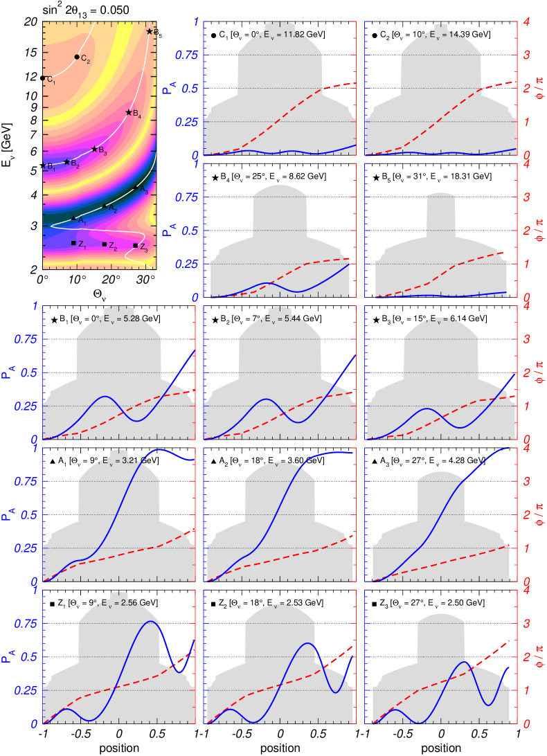
Figure 5: Dependence of the probability $P_{A}$ (solid blue), half-phase $\phi$ (dashed red) and the Earth density (gray shade) on the position along the neutrino trajectory, for $\sin^{2}2\theta_{13}=0.05$ and different values of $\Theta_{\nu}$ and $E_{\nu}$. The corresponding points of the oscillogram, together with the curves of the amplitude (collinearity) condition, are shown in the upper-left panel.

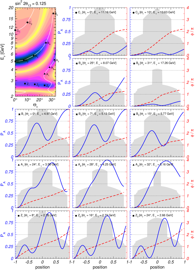
Figure 6: Same as in Fig. 5, but for $\sin^{2}2\theta_{13}=0.125$.

Core ridge. The core resonance ridge is located at $E_{\nu}\sim(2.5-2.8)$ GeV. It is of the MSW resonance nature, but is situated below the MSW resonance line in the core: $E_{\nu}<E_{R}(\Theta_{\nu})$, the reason being that the values of the oscillation half-phase are different from $\pi/2$. The ridge does not coincides with any curve corresponding to the phase or amplitude condition. At one point on the ridge there is an intersection of the curves $\mathop{\mathrm{Im}}\beta_{1}=0$ (the mantle half-phase $\phi_{1}=\pi$) and the collinearity condition, as well as of the $\mathop{\mathrm{Re}}\alpha_{2}=0$ curve, corresponding to the core half-phase $\phi_{2}=\pi/2$ (see Fig. 4). This crossing point corresponds to the local maximum with zero mantle effect and maximal oscillation amplitude in the core.

As follows from Figs. 5 and 6, the main contribution to the oscillation probability comes from the MSW-enhanced oscillations in the core, though the mantle contribution is not negligible. The detailed picture depends on the value of $\sin^{2}2\theta_{13}$.

For the inner core trajectories with $\Theta_{\nu}\sim 0$, the core phase $\phi_{2}>\pi/2$, and it decreases along the ridge with $\Theta_{\nu}$ increasing. For small mixing angles, e.g. $\sin^{2}2\theta_{13}\leq 0.05$ (see Fig. 5, lower panels), the contributions of the two mantle layers to $P_{A}$ practically cancel each other, so that the probability is determined by the oscillations in the core. The oscillation phase in the core, $\phi_{2}$, weakly decreases with the increase of $\Theta_{\nu}$, in spite of a substantial decrease of the trajectory length. The phase acquired in the core can be written as

$$\phi_{2}=\frac{\pi L_{2}(\Theta_{\nu})}{l_{m}(\bar{V}(\Theta_{\nu}))}\approx\text{const}\,,$$ (81)

where $\bar{V}(\Theta_{\nu})$ is the value of the potential averaged along a given trajectory and $L_{2}(\Theta_{\nu})=2R_{c}\cos\Theta_{\nu}$ is the neutrino path length inside the core. The ridge is below the resonance and therefore the oscillation length in matter decreases sharply (for small mixing) with the potential and also with energy. With the increase of $\Theta_{\nu}$ the length of the core-trajectory $L_{2}$ decreases, but simultaneously, the oscillation length decreases since the average potential decreases according to the PREM profile. These two dependencies compensate each other in Eq. (81) leading to weak change of $\phi_{2}$.

At $\Theta_{\nu}=27^{\circ}$ (point $Z_{3}$) the phase reaches $\phi_{2}=\pi/2$ and furthermore $\phi_{1}=\pi$. This corresponds to pure core effect. Notice that with increase of $\Theta_{\nu}$ the average density decreases and the depth of oscillations becomes smaller. In Fig. 7b we show the graphical representation of evolution with parameters from core-ridge (point $Z_{3}$). We show the precession cones in the mantle and in the core in the points close to border between the mantle and core. Shift of the evolution trajectory from the cone surfaces is due to density change and violation of adiabaticity.

For $\sin^{2}2\theta_{13}=0.05$ another intersection of lines of the amplitude condition and the phase conditions $\mathop{\mathrm{Re}}\alpha_{2}=0$ (core half-phase $\pi/2$) occurs at $E_{\nu}=3.3$ GeV and $\Theta_{\nu}=10^{\circ}$. Evolution for this configuration is shown in Fig. 5 point $A_{1}$. Notice that this point is in the ridge $A$. Here transitions in both mantle layers are non-zero but have opposite sign and cancel each other. So, the whole effect due to MSW resonance enhancement in core.

For large 1-3 mixing, e.g. $\sin^{2}2\theta_{13}=0.125$, there is substantial interplay of the core and mantle oscillation effects (see Fig. 6). For $\Theta_{\nu}\sim 0$, we find $\phi_{1}\sim\phi_{2}<\pi$; contributions from two mantle layers interfere constructively and the total mantle contribution is comparable with the core contribution (the later is resonantly enhanced). With increase of $\Theta_{\nu}$, the phase $\phi_{1}$ increases reaching $\pi$, whereas $\phi_{2}$ decreases. Mantle contribution decreases, and moreover, effects of two mantle layers start to compensate each other. At $\Theta_{\nu}=29^{\circ}$ the condition of local maximum are satisfied.

Notice that for large $\sin^{2}2\theta_{13}$ the decrease of $l_{m}$ with $\bar{V}$ is weaker and therefore it can not compensate decrease of the trajectory length. The phase stays constant if also the energy decreases. Consequently, for $\sin^{2}2\theta_{13}>0.05$ the energy of ridge line decreases with increase of $\Theta_{\nu}$. Even stronger dependence of the energy on $\Theta_{\nu}$ can be seen in the case of constant density in the core.

Recall that in this domain of low energies the oscillations due to 1-2 splitting become important [37].

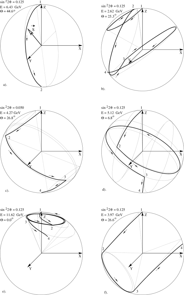
Figure 7: Graphical representation of neutrino evolution in the Earth. Shown are the trajectories of the neutrino vector $\vec{s}$ in the $(X,\,Y,\,Z)$ space (solid lines), for different values of $\theta_{13}$ and different points in the oscillograms. The different panels correspond to a) the MSW peak in mantle; b) the point $Z_{2}$ in Fig. 6; c) the point $A_{3}$ in Fig. 5; d) the point $B_{2}$ in Fig. 6; e) the point $C_{1}$ in Fig. 6; f) near saddle point $A_{1}$ in Fig. 6. We also show the precession cones (dotted lines) in the mantle and core points close to the border between the mantle and core. Sections 1-2, 2-3 and 3-4 indicate evolution in the first mantle layer, the core and the second mantle layer correspondingly.

The parametric ridges differ by the oscillation phase acquired in the core, $\phi_{2}$.

Ridge A. The phase in the core $\phi_{2}\lesssim\pi$. This ridge lies in between the core resonance (at $\Theta_{\nu}\sim 0^{\circ}$) and the mantle resonance regions. At the border between the core and the mantle domains of the oscillogram, $\Theta_{\nu}=33.1^{\circ}$, this ridge merges with the MSW resonance peak in the mantle.

This ridge is large (has the largest area of probability close to 1) for small 1-3 mixing: $\sin^{2}2\theta_{13}\lesssim 0.05$. As we mentioned above, for $\Theta_{\nu}<10^{\circ}$ and $E_{\nu}\sim 3$ GeV the phase in the core $\phi_{2}<\pi/2$, the mantle effect is small and two mantle layer contributions cancel each other. So, here we deal with resonance enhancement of oscillations in core. With increase of $E_{\nu}$ and $\Theta_{\nu}$ along the ridge both phases $\phi_{1}$ and $\phi_{2}$ decrease. The core and two mantle contributions add constructively leading to large probability. For example, for the point $A_{3}$ (Fig 5) $\pi_{1}\approx\pi_{2}\approx\pi/3$ and maximal probability build up by three comparable contributions. The graphical representation of this evolution is shown Fig. 7c. For the core part we show in some panels two precession cones, corresponding to the beginning and the end of the core section. The difference of these two cones reflects the effects of the non-constant density distribution.

For large 1-3 mixing $\sin^{2}2\theta_{13}\geq 0.075$, the region of maximal transition shifts to the mantle domain. Furthermore, the saddle point appear between the MSW resonance and the parametric resonance regions. In the saddle point $A_{1}$ (Fig. 6) the phases in the core and the mantle $\phi_{1}\approx\phi_{2}\approx\pi/2$, correspond to maximal oscillatory factors. However the contributions from the two mantle layers have opposite sign and cancel each other. The corresponding graphical representation is shown in Fig. 7f.

With increase of $\Theta_{\nu}$ the phases $\phi_{1}$ and $\phi_{2}$ decrease and cancellation becomes weaker.

In the ridge $A$ for small 1-3 mixing the lines of the phase and amplitude conditions almost coincide that ensures stability of enhancement in large area. This stability can be understood also in the following way. With increasing $\Theta_{\nu}$, the core segment of the trajectory becomes shorter and the mantle ones become longer. This is compensated by an increase of energy along the ridge. Indeed, since the ridge $A$ is between the core and the mantle MSW resonance energies, with an increase of energy the oscillation length in the core (above the MSW resonance) decreases, whereas the oscillation length in the mantle (below the mantle MSW resonance) increases, so that the oscillation phases change rather weakly. Along the ridge, in the direction of larger $\Theta_{\nu}$ the depth of oscillations in the core decreases, and this is compensated by an increase of the depth in the mantle. All this produces a long ridge and ensures its stability.

Ridge B. This ridge is situated at $E_{\nu}\geq 5$ GeV. For the smallest energies in the ridge and $\Theta_{\nu}\sim 0$ the half-phase in the core $\phi_{2}\sim(1.2-1.3)\pi$, so that oscillations in the core give substantial contribution effect (see Figs. 5 and 6). In the range $E_{\nu}=(5-6)$ GeV the parametric enhancement of oscillations with significant interplay of the core and mantle oscillation effects is realized. In Fig. 7d we show graphical representation for the point $B_{2}$ (Fig. 6).

With increase of $\Theta_{\nu}$ and $E_{\nu}$ the phase $\phi_{2}$ decreases due to decrease of the trajectory length $L_{2}$ (notice that here $l_{m}$ decreases too approaching $l_{0}$ but much weaker than $L_{2}$.) In contrast, the phase in the mantle increases. For $E_{\nu}=(6-7)$ GeV one finds $\phi_{2}\approx\pi$ an the core effect is absent, so that transition occurs due to the oscillations in mantle only.

For $E_{\nu}>20$ GeV the equality $\phi_{2}\sim\phi_{1}\sim\pi/2$ is realized. Indeed, the lines $\mathop{\mathrm{Re}}\alpha_{1}$ and $\mathop{\mathrm{Re}}\alpha_{2}$ as well as lines of the amplitude and phase conditions cross in the point $E_{\nu}\approx 21$ GeV and $\Theta_{\nu}=31^{\circ}$. Here maximal enhancement of the transition probability for given values of mixing angles occurs [25]. It is described by Eq. (69).

With an increase of both $E_{\nu}$ and $\Theta_{\nu}$ along the ridge the oscillation amplitudes decrease both in the core and in the mantle layers. The core-oscillation depth is suppressed stronger and therefore the region of relatively high probability lies in the same energy domain as the region of high probability in the mantle.

In this ridge a qualitative picture of oscillations does not depend on $\sin^{2}2\theta_{13}$.

Ridge C. The ridge is located at $E_{\nu}>11$ GeV in the matter dominated region where mixing and consequently oscillation depth are suppressed. For $\Theta_{\nu}\sim 0$ the half-phase in the core equals $\phi_{2}\sim 1.8\pi$. Here main contribution to probability is due to oscillations in mantle whereas the core gives small (negative) contribution. We show graphical representation of evolution that corresponds to the point $C_{1}$ in Fig. 7e.

With increase of $\Theta_{\nu}$ and $E_{\nu}$ along the ridge the phase $\phi_{2}$ decreases and the $E_{\nu}>100$ GeV reaches $3\pi/2$, whereas the mantle phase is about $\phi_{1}\sim\pi/2$. Here, as in the case of ridge $B$, the parametric enhancement of oscillations is realized [25] as described by the Eq. (69).

Notice that qualitative features of the high energy part of ridge $B$ and ridge $C$ do not depend on $\theta_{13}$ since both are in the $\theta_{13}$ factorization region where $P_{A}\propto\sin^{2}2\theta_{13}$ (see Sec. 5.1).

4 Approximate analytic description of neutrino oscillations in the Earth

In this section we develop an approximate analytic approach to 2-flavor neutrino oscillations in the Earth. To this end, we employ a perturbation theory in the deviation of the density profile from that represented by layers of constant densities. This approach has been first developed in Ref. [30] for the description of the solar neutrino oscillations in the earth. Here we apply it to the study of atmospheric neutrinos. The approximation turns out to work extremely well in spite of the fact that the variations of the neutrino potential inside the Earth layers can be large $|\Delta V|/\bar{V}\sim 0.3$. The high accuracy of our approach is related to the symmetry of the density profile of the Earth.

4.1 Perturbation theory in $\Delta V$

Let us first consider the case of one layer of relatively weakly varying density and represent the matter-induced potential of neutrinos $V(x)$ along a given trajectory as the sum of a constant term $\bar{V}$ and a perturbation $\Delta V(x)$:

$$V(x)=\bar{V}+\Delta V(x)\,.$$ (82)

Correspondingly, the Hamiltonian of the system can be written as the sum of two terms:

$$H(x)=\bar{H}+\Delta H(x)\,,$$ (83)

where

$$\bar{H}\equiv\bar{\omega}\begin{pmatrix}-\cos 2\bar{\theta}&\sin 2\bar{\theta}\\ \hphantom{-}\sin 2\bar{\theta}&\cos 2\bar{\theta}\end{pmatrix},\qquad\Delta H\equiv\frac{\Delta V(x)}{2}\begin{pmatrix}1&\hphantom{-}0\\ 0&-1\end{pmatrix}\,.$$ (84)

Here $\bar{\theta}=\theta_{m}(\bar{V})$ is the mixing angle in matter and $\bar{\omega}=\omega(\bar{V})$ is half of the energy splitting (half-frequency) in matter, both with the average potential $\bar{V}$. Throughout this chapter we will denote by $\bar{S}(x)$ the evolution matrix of the system for the constant density case $H(x)=\bar{H}$. The explicit expression for $\bar{S}(x)$ is given by Eq. (20) with $\theta_{m}=\bar{\theta}$.

For matter of varying density, we seek the solution of the evolution equation (3) in the form

$$S(x)=\bar{S}(x)+\Delta S(x),\qquad\Delta S(x)=-i\,\bar{S}(x)\,K_{1}(x)\,,$$ (85)

where $K_{1}(x)$ satisfies $|K_{1}(x)_{ab}|\ll 1$. Inserting Eq. (85) into Eq. (3), we find the following equation for $K_{1}(x)$ to the first order in $\Delta H(x)$ and $K_{1}(x)$:

$$\frac{dK_{1}(x)}{dx}=\bar{S}^{\dagger}(x)\,\Delta H(x)\,\bar{S}(x)=\frac{\Delta V(x)}{2}\left\{-\cos 2\bar{\theta}\begin{pmatrix}-\cos 2\bar{\theta}&\sin 2\bar{\theta}\\ \hphantom{-}\sin 2\bar{\theta}&\cos 2\bar{\theta}\end{pmatrix}\right.\\[5.69054pt] \left.+\sin 2\bar{\theta}\begin{pmatrix}\sin 2\bar{\theta}&\hphantom{-}\cos 2\bar{\theta}\\ \cos 2\bar{\theta}&-\sin 2\bar{\theta}\end{pmatrix}\cos 2\phi(x)+\sin 2\bar{\theta}\begin{pmatrix}0&-i\\ i&\hphantom{-}0\end{pmatrix}\sin 2\phi(x)\right\}\,.$$ (86)

The first term does not contribute to $S\equiv S(L)$ since $\langle\Delta V\rangle\equiv\int\Delta V(x)dx=0$, and Eq. (86) can be immediately integrated:

$$K_{1}(L)=\frac{1}{2}\sin 2\bar{\theta}\left\{\begin{pmatrix}\sin 2\bar{\theta}&\hphantom{-}\cos 2\bar{\theta}\\ \cos 2\bar{\theta}&-\sin 2\bar{\theta}\end{pmatrix}\int_{0}^{L}\Delta V(x)\,\cos 2\phi(x)\,dx\right.\\ \left.+\begin{pmatrix}0&-i\\ i&\hphantom{-}0\end{pmatrix}\int_{0}^{L}\Delta V(x)\,\sin 2\phi(x)\,dx\right\}\,.$$ (87)

It is convenient to introduce the new variable $z=x-L/2$, which measures the distance from the midpoint of the neutrino trajectory. Then from (87) we obtain

$$\Delta S\equiv\Delta S(L)=-i\,\sin 2\bar{\theta}\left\{\begin{pmatrix}\sin 2\bar{\theta}&\hphantom{-}\cos 2\bar{\theta}\\ \cos 2\bar{\theta}&-\sin 2\bar{\theta}\end{pmatrix}\Delta I+\begin{pmatrix}0&-i\\ i&\hphantom{-}0\end{pmatrix}\Delta J\right\}\,,$$ (88)

where

$$\Delta I\equiv\frac{1}{2}\int_{-L/2}^{L/2}\Delta V(z)\,\cos(2\bar{\omega}z)\,dz\,,\qquad\Delta J\equiv\frac{1}{2}\int_{-L/2}^{L/2}\Delta V(z)\,\sin(2\bar{\omega}z)\,dz\,.$$ (89)

In these integrals, $\Delta V(z)\equiv\Delta V(x(z))$ and $x(z)=z-L/2$. Obviously, $\Delta J$ vanishes if the perturbation $\Delta V(z)$ is symmetric with respect to the midpoint of the trajectory. Analogously, $\Delta I$ vanishes if $\Delta V(z)$ is antisymmetric. The expression for $S$ defined in Eq. (85) with $\Delta S$ given in Eqs. (88) and (89) is equivalent to Eqs. (13–16) obtained in Ref. [30] in the context of solar neutrino oscillations.

Let us now consider the issue of the unitarity of the obtained evolution matrix that can be important for numerical calculations. Since $\bar{S}\equiv\bar{S}(L)$ is unitary, we have

$$S^{\dagger}S=I+\Delta S^{\dagger}\bar{S}+\bar{S}^{\dagger}\Delta S+\Delta S^{\dagger}\Delta S.$$ (90)

The second and third terms on the RHS of this equality cancel each other thus ensuring the unitarity of $S$ at the first order in $\Delta S$. In order to prove this it is convenient to parametrize the evolution matrix $\bar{S}$ and the perturbation $\Delta S$ (88) as in Eq. (40):

$$Y =\cos\phi\,, \mathbf{X} =\sin\phi\left(\sin 2\bar{\theta},\;0,\;-\cos 2\bar{\theta}\right)\,,$$ (91)

$$\Delta Y =0, \Delta\mathbf{X} =\varepsilon\left(\cos 2\bar{\theta}\,\cos\xi,\;\sin\xi,\;\sin 2\bar{\theta}\,\cos\xi\right)\,,$$ (92)

where $\phi\equiv\phi(L)$ and we have introduced

$$\varepsilon=\sin 2\bar{\theta}\,\sqrt{\Delta I^{2}+\Delta J^{2}}\,,\qquad\xi=\arg(\Delta I+i\,\Delta J)\,.$$ (93)

It is easy to see that $\Delta S^{\dagger}\bar{S}+\bar{S}^{\dagger}\Delta S=Y\,\Delta Y+\mathbf{X}\cdot\Delta\mathbf{X}=0$. The last term in Eq. (90), $\Delta S^{\dagger}\Delta S$, violates the unitarity condition, however it is of order $\varepsilon^{2}$ and therefore it does not break consistency of our approximation. However, for practical purposes it would be useful to have an expression for $S$ which is exactly unitary regardless of the size of the perturbation, even if for large perturbations the formalism is no longer accurate. In order to do this, we first rewrite Eq. (88) as follows:

$$\Delta S=\varepsilon\,S^{\prime}\,,\qquad S^{\prime}=-i\left\{\begin{pmatrix}\sin 2\bar{\theta}&\hphantom{-}\cos 2\bar{\theta}\\ \cos 2\bar{\theta}&-\sin 2\bar{\theta}\end{pmatrix}\cos\xi+\begin{pmatrix}0&-i\\ i&\hphantom{-}0\end{pmatrix}\sin\xi\right\}\,,$$ (94)

and then we perform the following replacement in the expression for $S$:

$$S=\bar{S}+\varepsilon\,S^{\prime}\quad\longrightarrow\quad S=\cos\varepsilon\,\bar{S}+\sin\varepsilon\,S^{\prime}\,.$$ (95)

Note that both $S^{\prime}$ and $\bar{S}$ are unitary matrices, and that due to their specific form the combination on the right-hand-side of Eq. (95) is exactly unitary. In our computations we use the exactly unitary matrix (95).

4.2 Application: mantle-only crossing trajectories

We shall now use the formalism of the previous subsection to derive an explicit formula for the transition probability for mantle-only crossing neutrino trajectories. Since the density profile is symmetric with respect to the midpoint of the trajectory, the term $\Delta J$ is absent. From Eqs. (20), (88) and (95) we immediately get

$$P_{A}=\left[\cos\varepsilon\,\sin 2\bar{\theta}\,\sin\phi+\sin\varepsilon\,\cos 2\bar{\theta}\right]^{2}\approx\sin^{2}2\bar{\theta}\,\left[\sin\phi+\Delta I\,\cos 2\bar{\theta}\right]^{2},$$ (96)

where $\varepsilon\equiv\sin 2\bar{\theta}\,\Delta I$ and $\phi\equiv\phi(L)=\bar{\omega}L$. Here the first term in the square brackets describes oscillations in constant density matter with average potential $\bar{V}_{1}$. In order to obtain an explicit formula for $\Delta I$, we approximate the matter density profile along the neutrino trajectory by a parabola:

$$\Delta V(z)\approx V^{\prime\prime}_{1}\left[\left(\frac{z}{L}\right)^{2}-\frac{1}{12}\right].$$ (97)

The average value $\bar{V}_{1}$ and the coefficient $V^{\prime\prime}_{1}$ depend only on the nadir angle $\Theta_{\nu}$, and are shown in Fig. 8. Inserting the expression for $\Delta V(z)$ into Eq. (89) and integrating by parts, we obtain

$$\Delta I=\frac{V^{\prime\prime}_{1}L}{12}f(\phi),\qquad f(\phi)\equiv\frac{3\phi\cos\phi+(\phi^{2}-3)\sin\phi}{\phi^{3}}\,.$$ (98)

The function $f(\phi)$ has the following features: for $\phi\rightarrow 0$ (outer trajectories), one has $f(\phi)\rightarrow-\phi^{2}/15$; for $\phi=\pi/2$ which corresponds to the maximum transition probability for a given mixing angle in matter, $f(\phi)\approx-0.13$; the function $|f(\phi)|$ reaches its maximum, $f(\phi)\approx-0.31$, at $\phi\simeq 1.07\pi$. The function $f(\phi)$ changes its sign at $\phi\sim 1.8\pi$, and for large $\phi$ it behaves as $f(\phi)\sim\sin\phi/\phi$.

From Eqs. (96) and (98) it follows that:

• in the zeroth approximation, the transition probability is given by the standard oscillation formula for matter of constant density, with the oscillation amplitude determined by the mixing angle $\bar{\theta}=\theta_{m}(\bar{V}_{1})$ and the phase $\phi=\omega(\bar{V}_{1})L$;

• the lowest-order correction to $P_{A}$ vanishes at the MSW resonance, i.e. along the curve $E_{R}(\Theta_{\nu})$. The correction changes its sign at the resonance, being positive below it ($E_{\nu}<E_{R}(\Theta_{\nu}))$ and negative above it;

• the largest corrections correspond to the trajectories with $\Theta_{\nu}\sim 37^{\circ}$ (i.e. passing close to the core) and the phase $\phi\sim\pi$. Indeed, $f(\phi)$, $|V^{\prime\prime}_{1}|$ and $L$ are all maximal for the deepest mantle trajectories

The transition probability defined by Eqs. (96) and (98) can be cast into the form resembling formally the standard oscillation probability in vacuum or in matter of constant density:

$$P_{A}=\sin^{2}2\theta^{\prime}\,\sin^{2}\phi^{\prime}\,,$$ (99)

where

$$\sin^{2}2\theta^{\prime}\equiv(a^{2}+b^{2})\sin^{2}2\bar{\theta},\qquad\phi^{\prime}=\phi+\arctan(a/b)$$ (100)

with

$$a=\frac{V^{\prime\prime}_{1}L}{4\phi^{2}}\cos 2\bar{\theta}\,,\qquad b=1+V^{\prime\prime}_{1}L\frac{\phi^{2}-3}{12\phi^{3}}\cos 2\bar{\theta}\,.$$ (101)

This representation has the advantage that it factorizes the transition probability into a smooth function of neutrino energy and nadir angle, $\sin^{2}2\theta^{\prime}$, and the oscillating factor $\sin^{2}\phi^{\prime}$ lying between 0 and 1. In particular, zero probability curves in the oscillograms are given by the condition $\phi^{\prime}(\Theta_{\nu},E_{\nu})=\pi k$. Factorization shows immediately continuous character of lines of zero probability. Note that the effective oscillation amplitude $\sin^{2}2\theta^{\prime}$ is not actually a sine squared of any angle and should be simply understood as a notation defined in Eq. (100); in particular, it is not bounded from above by unity.

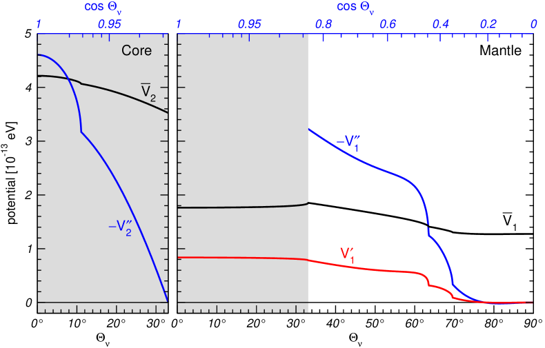
Figure 8: Dependence of the average potentials ($\bar{V}_{1}$, $\bar{V}_{2})$ (black) as well as the coefficients $V^{\prime}_{1}$ (red) and ($-V^{\prime\prime}_{1}$, $-V^{\prime\prime}_{2}$) (blue) on the nadir angle $\Theta_{\nu}$.

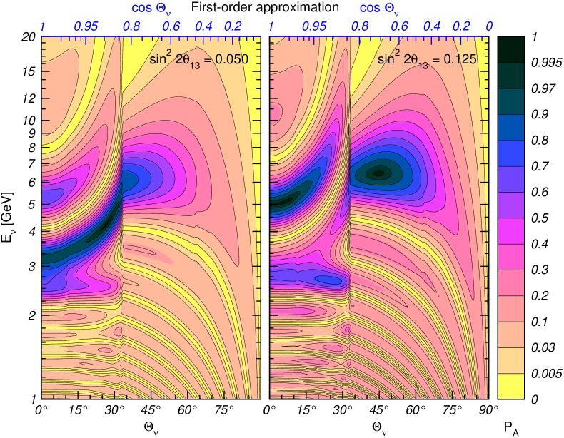
Figure 9: Contour plot of the probability $P_{A}$ for the PREM density profile (colored regions; grayscale on black-and-white printouts) and for our analytic approximation including first-order corrections (black curves).

4.3 Application: core-crossing trajectories

For trajectories crossing the Earth’s core, the evolution matrix can be factorized as

$$S=S_{1}^{T}\,S_{2}\,S_{1}\,,$$ (102)

where the subscripts ‘$1$’ and ‘$2$’ refer to the mantle (one layer) and core. $S_{1}$ and $S_{2}$ can be calculated using the formalism described in the previous sections. Since the core density profile is symmetric, the corresponding integral $\Delta J_{2}$ vanishes, whereas $\Delta I_{2}$ can be calculated in full analogy with the derivation of $\Delta I$ in Sec. 4.2. In particular, we can approximate the core density profile by a parabola and obtain for $\Delta I_{2}$ an expression which is completely analogous to that in Eq. (98): $\Delta I_{2}=\Delta I(\phi_{2},V_{2}^{\prime\prime}L_{2})$. Here $\phi_{2}\equiv\bar{\omega}_{2}L_{2}$ is the phase acquired in the core layer. The expression for $S_{2}$ is therefore

$$S_{2}=\cos\varepsilon_{2}\,\bar{S}_{2}-i\,\sin\varepsilon_{2}\begin{pmatrix}\sin 2\bar{\theta}_{2}&\hphantom{-}\cos 2\bar{\theta}_{2}\\ \cos 2\bar{\theta}_{2}&-\sin 2\bar{\theta}_{2}\end{pmatrix},\qquad\varepsilon_{2}=\sin 2\bar{\theta}_{2}\,\Delta I_{2}\,.$$ (103)

For the neutrino trajectories that cross the Earth’s core, it is convenient to approximate the density profile within each mantle layer by a linear function of the coordinate:

$$V_{1}(z)=\bar{V}_{1}+\Delta V_{1}(z),\qquad\Delta V_{1}(z)\approx V^{\prime}_{1}\frac{z}{L_{1}}\,,$$ (104)

where $L_{1}$ is the length of one mantle layer. The advantage of this parametrization is that $\Delta V_{1}(z)$ is an antisymmetric function of $z$, and therefore $\Delta I_{1}$ vanishes. For $\Delta J_{1}$ we obtain from Eq. (89):

$$\Delta J_{1}=V^{\prime}_{1}L_{1}\,\frac{\sin\phi_{1}-\phi_{1}\cos\phi_{1}}{4\phi_{1}^{2}}\,$$ (105)

where $\phi_{1}\equiv\bar{\omega}_{1}L_{1}$ is the phase acquired in each mantle layer. Then $S_{1}$ is given by

$$S_{1}=\cos\varepsilon_{1}\,\bar{S}_{1}+\sin\varepsilon_{1}\begin{pmatrix}0&-1\\ 1&\hphantom{-}0\end{pmatrix},\qquad\varepsilon_{1}=\sin 2\bar{\theta}_{1}\,\Delta J_{1}\,.$$ (106)

At first-order in $\varepsilon_{1}$:

$$S_{1}\approx\begin{pmatrix}\cos\phi_{1}+i\cos 2\bar{\theta}_{1}\,\sin\phi_{1}&\sin 2\bar{\theta}_{1}\left(-i\sin\phi_{1}-\Delta J_{1}\right)\\ \sin 2\bar{\theta}_{1}\left(-i\sin\phi_{1}+\Delta J_{1}\right)&\cos\phi_{1}-i\cos 2\bar{\theta}_{1}\,\sin\phi_{1}\end{pmatrix}.$$ (107)

In Fig. 8 we show the dependence of ($\bar{V}_{1}$, $V^{\prime}_{1}$) and ($\bar{V}_{2}$, $V^{\prime\prime}_{2}$) on the nadir angle $\Theta_{\nu}$. With these functions, one can find from Eqs. (98) and Eqs. (105) the quantities $\Delta I_{2}$ and $\Delta J_{1}$ and then from Eqs. (103) and (106) the evolution matrices $S_{1}$ and $S_{2}$. Substituting the results into Eq. (102), one obtains the evolution matrix for the whole trajectory.

In the limit $|\Delta J_{1}|\ll|\sin\phi_{1}|$ Eq. (107) can be rewritten as

$$S_{1}=D_{1}\,\bar{S}_{1}\ D_{1}^{*}\,,\qquad D_{1}\equiv\begin{pmatrix}e^{-i\tau_{1}/2}&0\\ 0&e^{+i\tau_{1}/2}\end{pmatrix}\,,\qquad\tau_{1}=\arcsin\left(\frac{\Delta J_{1}}{\sin\phi_{1}}\right)\,,$$ (108)

and since $\Delta J_{1}$ is real, $D_{1}$ is a pure phase matrix. In this limit the total evolution matrix Eq. (102) takes the form

$$S=\bar{S}_{1}\,D_{1}\,S_{2}\,D_{1}\,\bar{S}_{1}\,$$ (109)

where we have omitted the two outer matrices $D_{1}^{*}$ are irrelevant for the calculation of $P_{A}=|S_{12}|^{2}$. The two matrices $D_{1}$ in Eq. (109) can be combined with $S_{2}$ to construct an effective core matrix, which takes into account all the first-order corrections (both in the core and in the mantle):

$$S\equiv\bar{S}_{1}\,S^{\prime}_{2}\,\bar{S}_{1}\,,\qquad S^{\prime}_{2}\equiv D_{1}\,S_{2}\,D_{1}\,.$$ (110)

An advantage of this approach is that both $\bar{S}_{1}$ and $S^{\prime}_{2}$ are symmetric matrices, so that all the results derived previously in the constant-density approximation can be improved to take into account the first-order corrections by simply replacing $\bar{S}_{2}\to S^{\prime}_{2}$. The asymmetry of the mantle profile is effectively resolved.

In Fig. 9 we compare the $P_{A}$ oscillograms obtained by numerical calculations for the PREM matter profile with those obtained using Eqs. (102), (103) and (106). As can be seen from this figure the degree of accuracy increases drastically once the corrections described here are included.

An advantage of the described approximate analytic approach is that the coefficients $\bar{V}$ and $V^{\prime\prime}_{1}$ depend solely on the nadir angle of the neutrino trajectory $\Theta_{\nu}$. In particular, they do not depend on neutrino energy and on the values of $\Delta m^{2}$ and $\theta$.

5 Dependence of oscillograms on 1-3 mixing, density profile and flavor channel

5.1 Dependence of oscillograms on 1-3 mixing

As can be seen in Fig. 1, with increasing $\sin^{2}2\theta_{13}$ the oscillation probability increases everywhere in the $(E_{\nu},\,\Theta_{\nu})$ plane. The evolution of the oscillation pattern appears as a “flow” of higher probability along nearly fixed curves towards larger values of $\Theta_{\nu}$: The flow is along the curves of the phase condition (57) for the mantle trajectories, and along the curves of the collinearity condition for the core-crossing trajectories. These lines of flow move only weakly with $\theta_{13}$.

The region of sizable oscillation probability, $P_{A}\geq 1/2$, appears first for $\sin^{2}2\theta_{13}\approx 0.009$, at $\Theta_{\nu}=0^{\circ}$ and $E_{\nu}=2.8$ GeV. It is located on the parametric ridge $A$. This large probability is due to the parametric enhancement of the oscillations. With increase of $\sin^{2}2\theta_{13}$ the region of sizable probability expands along ridge $A$, and at $\sin^{2}2\theta_{13}\approx 0.025$ reaches the inner-mantle trajectories. At $\sin^{2}2\theta_{13}\approx 0.04$ the regions of $P_{A}\geq 1/2$ appear also (at $\Theta_{\nu}=0^{\circ}$) in the core MSW resonance region and in the parametric ridge $B$. The curves of zero oscillation probability change only very slightly with $\theta_{13}$. The nature of the increase of the oscillation probability with increasing $\theta_{13}$ is different in different regions of the parameter space.

Analytic expressions for various structures in the oscillograms, derived in Sec. 2.3, allow one to understand this evolution. Two features determine dependence of the oscillograms on 1-3 mixing:

• factorization of the $\theta_{13}$ dependent factors in the probability, and

• dependence of the amplitude and phase conditions on 1-3 mixing.

Let us consider first the regions outside the resonances: $E_{\nu}>E_{R}+\Delta E_{R}^{\text{max}}$, and $E_{\nu}<E_{R}-\Delta E_{R}^{\text{max}}$. Here $\Delta E_{R}^{\text{max}}=E_{R}\tan 2\theta_{13}^{\text{max}}$ and $\tan 2\theta_{13}^{\text{max}}\sim(0.1-0.2)$ corresponds to the maximal allowed values of 1-3 mixing. In practice, for the mantle-crossing trajectories these are the regions with $E_{\nu}<5$ GeV and $E_{\nu}>8$ GeV. In these regions, the mixing parameter in matter can be approximated by

$$\sin^{2}2\theta_{m}\approx\frac{\sin^{2}2\theta_{13}}{\left|1-\frac{2VE_{\nu}}{\Delta m^{2}}\right|^{2}},$$ (111)

Moreover, the half-phase

$$\phi\approx\frac{\Delta m^{2}}{4E_{\nu}}\left|1-\frac{2VE_{\nu}}{\Delta m^{2}}\right|L$$ (112)

does not depend on 1-3 mixing. So, for the mantle domain trajectories the lines of constant phase that determine the lines of flow do not depend on 1-3 mixing. As follows from (111) and (112), the oscillation probability for one layer (mantle) factorizes:

$$P_{A}\approx\sin^{2}2\theta_{13}\sin^{2}\phi\frac{1}{\left|1-2VE_{\nu}/\Delta m^{2}\right|^{2}}.$$ (113)

Therefore, the probability increases uniformly in the whole this area and the lines of zero and maximum transition probability do not move. For the core crossing trajectories similar analysis holds for $E_{\nu}<2$ GeV.

Let us first consider the parametric resonance condition (42) that determines approximately the lines of “flow”. Beyond the MSW resonance regions, the phases $\phi_{i}$, and therefore $c_{i}$ and $s_{i}$ ($i=1,2$), do not depend on the 1-3 mixing. The mixing angles in matter enter the condition as cosines $\cos 2\theta_{i}$. Outside the resonance regions $\theta_{i}\approx\theta_{13}\ll 1$ or $\theta_{i}\approx\pi/2$ and therefore $\cos 2\theta_{i}\approx\pm 1$ weakly depends on 1-3 mixing. So, the condition (and therefore the lines of flow) shifts only weakly with change of $\theta_{13}$.

Let us now consider the resonance regions $(2<E_{\nu}<12)$ GeV. Here dependence of the transition probability on $\sin^{2}2\theta_{13}$ is non-linear. Not only the depth of the oscillations, but also the oscillation length in matter in each layer depends on $\sin^{2}2\theta_{13}$ substantially, and the latter influences the interference effects. As a result, the transition probability changes with $\theta_{13}$ differently in different regions, and in addition the “lines of flow” shift.

• The MSW resonance peak in the mantle is determined by the condition (30). With increasing $\sin^{2}2\theta_{13}$, the peak shifts to larger values of $\Theta_{\nu}$ and to slightly larger energies. This can be readily understood. Indeed, the oscillation length at the resonance decreases with increasing $\theta_{13}$ as $l_{m}=l_{\nu}/\sin 2\theta_{13}$ and therefore the condition $\phi_{1}=\pi/2$ is satisfied for shorter (more external) trajectories. For these trajectories the average density becomes smaller, so that the resonance energy increases: $E_{R}\propto 1/\bar{V}$. The width of the resonance peak at half height increases as $\tan 2\theta_{13}$ both in neutrino energy and in $\Theta_{\nu}$ variables (see the discussion below Eq. (30)). Using the resonance condition (30), we obtain from (33)

  $$\tan 2\theta_{13}=\frac{\pi}{2\bar{V}(\Theta_{\nu})R\cos\Theta_{\nu}}\equiv\frac{\pi}{d}\,,$$ (114)

  where $d$ is the column density that corresponds to maximum of the transition probability. Eq. (114) gives an immediate relation between $\theta_{13}$ and the nadir angle of the neutrino trajectory on which the absolute maximum of the transition probability is realized. This can, in principle, be used for measuring $\theta_{13}$: the method would simply consist in the determination of $\Theta_{\nu}$ of the mantle-only crossing trajectory corresponding to the absolute maximum of the conversion probability $P_{A}=1-P_{ee}$.

• Core ridge slightly shifts with increase of $\theta_{13}$ to larger energies, especially at $\Theta_{\nu}\approx 0$.

• For ridge $A$, the region of sizable transition probability and the position of the maximum also move towards smaller $|\cos\Theta_{\nu}|$. With increasing $\theta_{13}$ the oscillation length decreases, especially in the resonance region. Therefore, the same phases in the core and mantle can be obtained for shorter trajectories in the core and therefore for larger $\Theta_{\nu}$.

• Ridge $B$ evolves weaker with $\theta_{13}$: the energy corresponding to the maximum of the transition probability stays rather close to that of the mantle MSW resonance, $E_{\nu}\approx(5-6)$ GeV. At higher energies the ridge is in the factorization region. With increase of $\theta_{13}$ at $\Theta_{\nu}\approx 0$ the ridge shifts to smaller $E_{\nu}$.

• The situation for ridge $C$ is similar to ridge $B$.

5.2 Dependence on the Earth’s density profile

In different parts of the $(E_{\nu},\,\Theta_{\nu})$ plane the oscillation probabilities have different sensitivity to the modifications of matter density profile. The sensitivity is very weak (independently of the form of perturbation) in the following parts:

• $\Theta_{\nu}>84^{\circ}$: here the length of the trajectory, and therefore the oscillation phase, are small, so that effect of “vacuum mimicking” [1, 5] takes place. To a good approximation matter does not affect the oscillation probabilities, irrespectively of whether or not the matter-induced potential $V$ is small compared to the kinetic energy difference $\Delta m^{2}_{31}/2E_{\nu}$.

• $E_{\nu}<2$ GeV: here one has $V\ll\Delta m^{2}_{31}/2E_{\nu}$, and so matter effects on the oscillations driven by 1-3 mixing and splitting are small for all values of $\Theta_{\nu}$.

The region of high sensitivity to the density profile of the Earth is bounded by $E_{\nu}>(3-4)$ GeV and $\Theta_{\nu}<66^{\circ}$. This is the region of energies close to and above the resonance energies (matter dominance) and of sufficiently long trajectories. The latter condition ensures an accumulation of the matter effects over long distances and therefore a sensitivity to large scale structures of the density profile. For the core-crossing trajectories the border of the sensitivity region is lower: $E_{\nu}\simeq 2$ GeV. Changes of the oscillograms in this region depend on the specific form of the modification of the matter density distribution.

For illustration, we consider here the effects of three different modifications of the Earth density profile: (1) replacing PREM profile by constant-density mantle and core layers, (2) modification of the core/mantle density ratio, and (3) changes of the position of the border between the mantle and the core.

1. In Fig. 2 we show the results of the fixed constant-density layers approximation, characterized by the constant potentials $V_{1}$ and $V_{2}$ in the mantle and core. This profile can be considered as an extreme case of flattening of the mantle and core density distributions. For the mantle-only crossing trajectories there are two lines in the oscillograms where the oscillation probabilities for the two profiles are equal: (i) $\Theta_{\nu}\approx 53^{\circ}$, which corresponds to the trajectory with $\bar{V}_{\rm PREM}={V}_{1}$, and (ii) the resonance energy curve $E_{\nu}\simeq E_{R}(\Theta_{\nu})$. Indeed, along the resonance curve the first-order correction to $P_{A}$ due to the deviation of the density profile from the averaged constant one disappears (see the discussion in Sec. 4.2).

For $\Theta_{\nu}<53^{\circ}$ the oscillation pattern for the fixed constant-density profile is shifted to higher energies compared to that for the PREM profile. Furthermore, for $E_{\nu}>E_{R}(\Theta_{\nu})$ one has $P_{\text{const}}>P_{\text{PREM}}$, whereas for lower energies, $E_{\nu}<E_{R}(\Theta_{\nu})$, $P_{\text{const}}<P_{\text{PREM}}$, which essentially reflects the shift of the resonance peak when profile is changed. The shift of contours in the energy scale increases as $\Theta_{\nu}$ decreases and reaches maximum for the deepest mantle trajectories. Quantitatively, in the high energy region, $E_{\nu}>6$ GeV, for $\Theta_{\nu}\sim 37^{\circ}$ the changes of probability equal $P_{\text{const}}/P_{\text{PREM}}=0.2/0.06$, $0.3/0.1$, $0.4/0.2$, $0.5/0.3$, $0.9/0.5$. That is, the modification is characterized by factor 2 - 3. The shift of contours in energy scale is about 1 GeV at $E_{\nu}\sim 10$ GeV. The differences between the results for the two profiles weakly depend on $\theta_{13}$. For $\Theta_{\nu}>53^{\circ}$, the PREM profile gives higher probabilities than those for the fixed constant-density layers approximation for $E_{\nu}>E_{R}(\Theta_{\nu})$ and lower probability for $E_{\nu}<E_{R}(\Theta_{\nu})$.

For core crossing trajectories the size of changes is similar.

2. Fig. 10 illustrates the effects of the increase (decrease) of the core density: $V_{2}(x)\rightarrow kV_{2}(x)$, where $k=const$. The shapes of the density profiles in the mantle and core are taken according to the PREM profile. The total mass of the Earth is unchanged and therefore the density of the mantle should be reduced (increased) correspondingly: $\Delta V_{1}/V_{1}=-[(R/R_{c})^{3}-1]^{-1}(\bar{V}_{2}/\bar{V}_{1})\Delta V_{2}/V_{2}\approx-0.3\Delta V_{2}/V_{2}$. The effects of the increase and decrease of the core potential on the oscillogram are opposite and for definiteness we will consider the case of an increase of $V_{2}$, so that for mantle-only crossing trajectories $V_{1}$ decreases. Since the resonance energy is proportional to $1/V$, a decrease of density leads to a shift of the resonance peak to higher energies and also to smaller $\Theta_{\nu}$, to satisfy the phase condition $\phi=\pi/2$. The strongest effect is for $\Theta_{\nu}<60^{\circ}$ and above the resonance. Quantitatively, a $\sim 6\%$ decrease of the mantle density (corresponding to the $20\%$ increase of $V_{2}$) leads, for $\Theta_{\nu}<37^{\circ}$, to an about 1 GeV upward shift of the contour curves. As follows from the figure, the increase of probabilities with respect to those for the PREM profile is $P_{\text{20\%}}/P_{\text{PREM}}=0.1/0.03$, $0.2/0.1,0.4/0.2$, $0.5/0.3,0.7/0.5$. The curve of unchanged probability is close to the resonance curve. Below the resonance energy the PREM profile leads to larger probabilities than the modified one.

Notice that these changes are rather similar to the changes for the constant-density layers profile. The reason is that in both cases in the inner parts of the mantle the density is smaller than that given by the PREM density profile.

The effect of density modifications on the transition probability is nearly linear in the variable of density change.

For core-crossing trajectories, an increase of the core density leads to a shift of the oscillatory pattern to larger $\Theta_{\nu}$ and higher energies, and also results in an increase of probability. These features can be understood using the parametric resonance condition.

3. Fig. 11 illustrates the effects of increase (decrease) of the core radius. Again, the requirement of keeping the total mass of the Earth fixed imposes a rescaling of the overall core and mantle densities. As in the previous case, this rescaling is what induces the most important effects on the oscillogram.

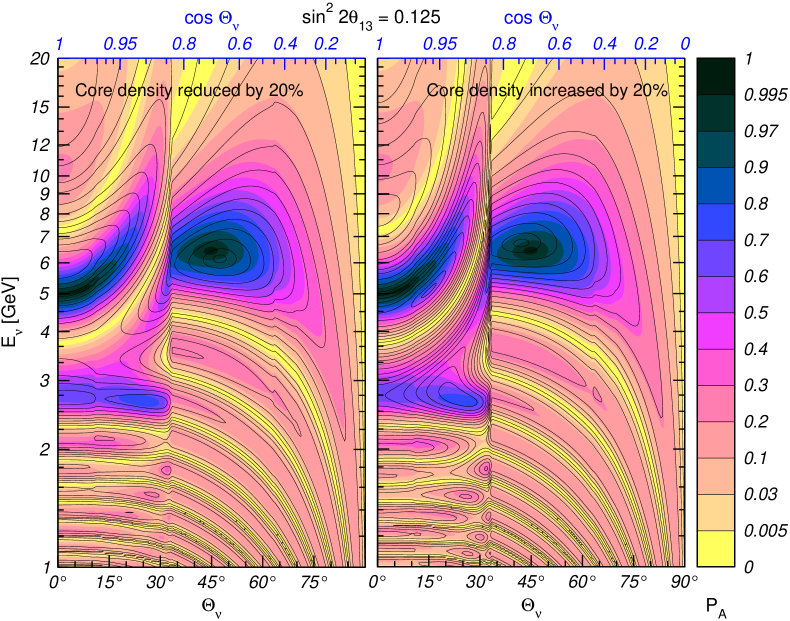
Figure 10: $P_{A}$ oscillograms for the PREM density profile (colored regions) and for a 20% variations of the core/mantle density ratio. The total mass of the Earth is kept fixed.

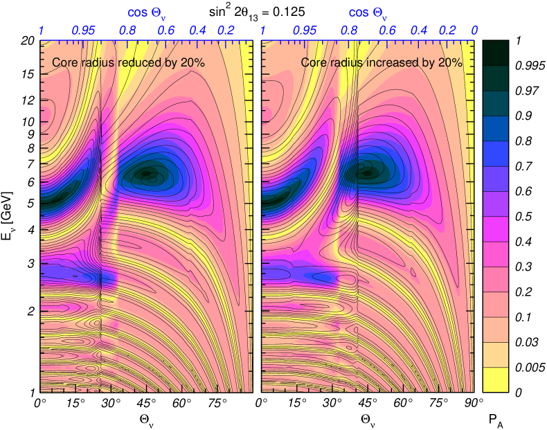
Figure 11: $P_{A}$ oscillograms for the PREM density profile (colored regions) and for a 20% variations of the core radius. The total mass of the Earth is kept fixed.

The sensitivity of the oscillation probabilities to the variations of the matter density distribution in the Earth can in principle be used for studying the Earth interior with neutrinos, i.e. to perform an oscillation tomography of the Earth [37]. Using the features described above one can work out the criteria for the selection of events that are sensitive to a given type of variations of the profile. For instance, in the case of flattening of the density distribution, one can divide the whole parameter space into 4 parts: (1) $\Theta_{\nu}<53^{\circ}$, $E_{\nu}>E_{R}$; (2) $\Theta_{\nu}>53^{\circ}$, $E_{\nu}<E_{R}$; (3) $\Theta_{\nu}<53^{\circ}$, $E_{\nu}<E_{R}$; (4) $\Theta_{\nu}>53^{\circ}$, $E_{\nu}>E_{R}$, and select a sample of the $e$-like events sensitive to these regions. The flat profile gives larger number of events then PREM profile in (1) and (2) regions and smaller number of events in the regions (3) and (4). This feature allows one to distinguish effect of flattening from other possible modifications of the profile as well as effect of uncertainty in $\theta_{13}$.

Notice that the changes of the oscillation probability due to modifications of the core/mantle density ratio and of the position of the border between the mantle and the core can be noticeable if the magnitude of the modifications is as large as $20\%$ (see Figs. 10 and 11). However, to detect them experimentally, the energy and nadir angle resolutions should be high as well as large event statistics is necessary. Therefore, the oscillation tomography of the Earth will put very challenging demands to future experiments.

5.3 Probabilities for other oscillation channels

In Figs. 12 and 13 we show the oscillograms for the other channels. As follows from the discussion in Sec. 2.2, in the approximation of zero 1-2 splitting ($\Delta m^{2}_{21}=0$) all the probabilities that involve $\nu_{e}$ depend on the single probability $P_{A}$. This is related to the fact that $\nu_{e}$ is unchanged upon going from the flavor basis to the propagation one.

The probability $P_{ee}=1-P_{A}$ is just complementary to $P_{A}$ with all the features inverted. $P_{e\mu}$ is just $P_{A}$ scaled by the factor $s^{2}_{23}$ (see the middle panel in Fig. 12). The maximal value of this transition probability is therefore $s^{2}_{23}$. Similarly, $P_{e\tau}$ is $P_{A}$ scaled by the factor $c^{2}_{23}$.

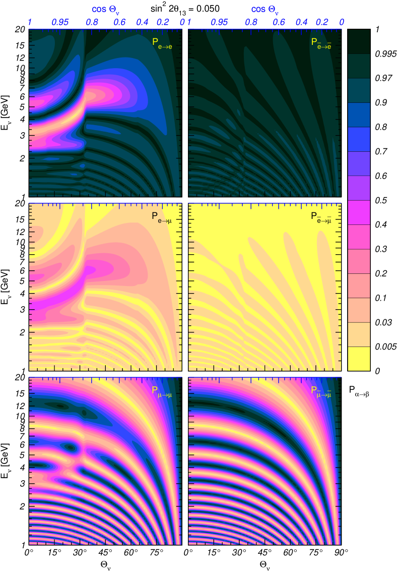
Figure 12: $P_{ee}$, $P_{e\mu}$ and $P_{\mu\mu}$ oscillograms, for neutrinos (left panels) and antineutrinos (right panels), $\sin^{2}2\theta_{13}=0.05$, $\sin^{2}2\theta_{23}=1$ and $\Delta m^{2}_{21}=0$.

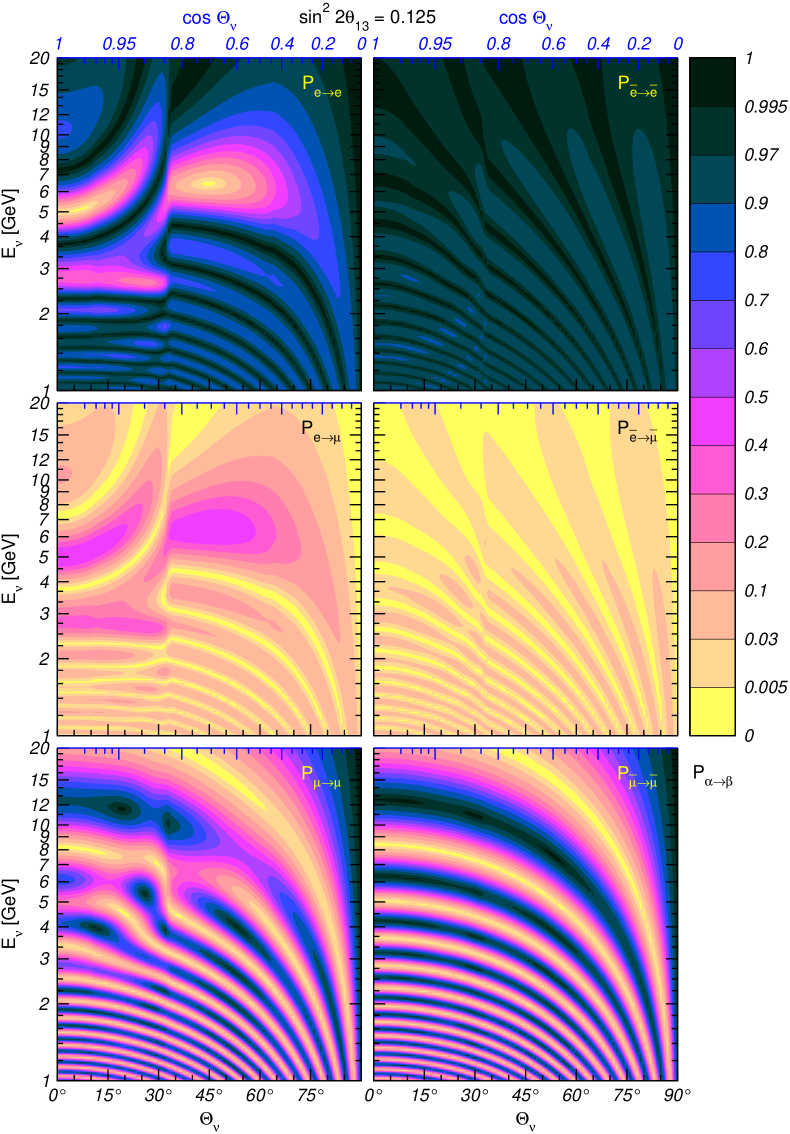
Figure 13: The same as in Fig. 12 but for $\sin^{2}2\theta_{13}=0.125$.

The probabilities of transitions that do not involve $\nu_{e}$ have more complicated structure since now both the initial and the final states do not belong to the propagation basis and therefore some additional interference occurs. The survival probability $P_{\mu\mu}$ in Eq. (16) can be written as

$$P_{\mu\mu}=P_{vac}-s^{4}_{23}P_{A}+2s^{2}_{23}c^{2}_{23}\,(\mathop{\mathrm{Re}}A_{33}-\cos 2\phi_{vac})\,,$$ (115)

where $P_{vac}=1-\sin^{2}2\theta_{23}\sin^{2}\phi_{vac}$ is the usual 2-flavor vacuum oscillation probability and $\phi_{vac}\equiv\Delta m^{2}_{31}L/4E_{\nu}$ is the vacuum oscillation phase. $P_{vac}$ describes the oscillation effect in the absence on the 1-3 mixing. The other two terms in (115) describe the effects of the 1-3 mixing. We can use the approximate results of Sec. 4 to estimate $\mathop{\mathrm{Re}}A_{33}$. Recall that in Sec. 4 we used a symmetric Hamiltonian for $2\nu$ system, which differs from the one introduced in Sec. 2.1 by a term proportional to the unit matrix (18). The term $\mathop{\mathrm{Re}}A_{33}$ essentially reflects evolution of the 1-3 system with respect to the state $\tilde{\nu}_{2}$ and so the $3\nu$ form of the Hamiltonian should be restored. According to Eq. (18) the relation between the corresponding evolution matrices (up to the removed decoupled state) is

$$\tilde{S}=e^{-i\psi}S,\qquad\psi\equiv\int_{0}^{L}\left(\frac{\Delta m^{2}_{31}}{4E_{\nu}}+\frac{V}{2}\right)dx\,.$$ (116)

Then

$$A_{33}=e^{-i\psi}\,S_{22}\,,$$ (117)

where $S_{22}$ is the 22 element of the matrix (20) with the correction given in (88).

Let us consider the mantle trajectories. Then from (117) we get explicitly

$$\mathop{\mathrm{Re}}A_{33}=\cos(\phi+\psi)+2\sin^{2}\bar{\theta}_{13}\sin\psi[\sin\phi+2\cos^{2}\bar{\theta}_{13}\Delta I]\,,$$ (118)

where the phase $\phi$ and the correction integral $\Delta I$ are defined in (20) and (89), respectively, and the angle $\bar{\theta}_{13}$ is the 1-3 mixing angle in matter calculated at the average value of the matter density. Then the survival probability $P_{\mu\mu}$ for the mantle-only crossing trajectory can be written as

$$P_{\mu\mu}=1-\sin^{2}2\theta_{23}\sin^{2}\left(\frac{\phi+\psi}{2}\right)-s_{23}^{4}P_{A}\\ +\frac{1}{2}\sin^{2}2\theta_{23}\sin\psi\left(2\sin^{2}\bar{\theta}_{13}\sin\phi+\sin^{2}2\bar{\theta}_{13}\,\Delta I\right)\,.$$ (119)

Notice that the first two terms here correspond to 2-flavor vacuum probability with the modified phase. The probability can be rewritten as

$$P_{\mu\mu}=P_{vac}+\Delta P$$ (120)

with

$$\Delta P=-s^{4}_{23}P_{A}-2s^{2}_{23}c^{2}_{23}\big{[}\cos 2\phi_{vac}-\cos(\phi+\psi)\\[2.84526pt] -2\sin^{2}\bar{\theta}_{13}\sin\psi\sin\phi-\sin^{2}2\bar{\theta}_{13}\sin\psi\,\Delta I\big{]}.$$ (121)

In the limit $s_{13}\to 0$ one has

$$\phi\approx\int_{0}^{L}\left(\frac{\Delta m^{2}}{4E_{\nu}}-\frac{V(x)}{2}\right)dx$$ (122)

which, together with (116), implies $\phi+\psi=2\phi_{vac}$.

These formulas can be used for the analysis of numerical results shown in Figs. 12 and 13. The first correction term in Eq. (121) is negative, so that it reduces the survival probability. The strongest effect of this mixing occurs in the resonance region. For high energies the 1-3 mixing is suppressed and $P_{\mu\mu}$ is again described well by the vacuum oscillation formula. Notice that in some regions with zero $P_{vac}$ the 1-3 mixing leads to the positive contribution which is due to the last term in (115) so that the lines of of zero probability are interrupted. Also there are no lines of maximal probability, as zero lines for $P_{A}$.

All the correction terms to $P_{vac}$ are in general of the same order; therefore the modification of the vacuum probability is rather complex and not immediately related to $P_{e\mu}$. The corrections are in general large in the regions of the parameter space where $P_{e\mu}$ is large, i.e. in the resonance regions and in the places of the resonance peaks and parametric ridges of $P_{A}$. Instead of continuous lines of maximal probability, in the case of non-zero 1-3 mixing one obtains saddle points and local maxima. In particular, the saddle point of the $P_{\mu\mu}$ probability appears in the mantle resonance region.

The structure of the transition probability $P_{\mu\tau}$ is similar to that of $P_{\mu\mu}$.

In the antineutrino channel, the 2-flavor probability $\bar{P}_{2}$ is suppressed by matter and the strongest transitions occur in the vacuum oscillation region. Some interference effects are seen for the core domain but no substantial parametric enhancement is realized.

6 Discussion and conclusions

1. We have worked out a detailed and comprehensive description of neutrino oscillations driven by non-zero 1-3 mixing inside the Earth. The description is given in terms of the oscillograms of the Earth: contours of constant oscillation probabilities in the $(E_{\nu},\,\Theta_{\nu})$ plane. In this first publication we have neglected the 1-2 mass splitting $\Delta m^{2}_{21}$, which is a good approximation for high neutrino energies, $E_{\nu}>1-2$ GeV.

2. We found that the oscillograms have a regular structure with several generic features: (i) the MSW peak in the mantle domain of the oscillogram; (ii) the MSW peak (ridge) in the core domain, (iii) three parametric ridges in the core domain; (iv) regular oscillatory pattern at low energies that has different features in the core and in the mantle domains of the oscillograms. We presented a detailed description of these structures: their position in the $(E_{\nu},\,\Theta_{\nu})$ plane, their evolution with changing 1-3 mixing and their dependence on the density profile of the Earth.

The most interesting features of the oscillograms appear at relatively high energies, $E_{\nu}=(2-12)$ GeV, and $\Theta_{\nu}<75^{\circ}$, i.e. in the resonance region. Notice that this region is not covered by the existing or forthcoming accelerator experiments, and on the other hand, statistics in the current atmospheric neutrino experiments is too low. All these experiments can only study very small effects on the “tails” of those interesting oscillation phenomena. Exploration of the resonance regions thus constitutes a significant experimental challenge for future experiments.

3. We studied the accuracy of the calculations based on the constant-density layers approximation to the Earth matter density profile. This approximation reproduces all the features of the oscillograms qualitatively well, though there are some quantitative differences and shifts of the structures in the $(E_{\nu},\,\Theta_{\nu})$ plane. The strongest deviations appear in the domain of deep mantle trajectories and high energies ($E_{\nu}>6$ GeV).

4. We showed that a complete physics interpretation of the oscillograms can be given in terms of different realizations of just two conditions: (i) the amplitude (or resonance) condition and (ii) the phase condition. In the case of one layer of constant density these conditions are reduced to the MSW resonance condition and half-phase equality $\phi=\pi/2+\pi k$. They determine the position of the absolute maxima of the transition probability. For three layers of constant densities the amplitude condition is reduced to the parametric resonance condition. This condition describes the position of the parametric ridges. The phase condition gives the position of the maximum along the ridge.

We show that the parametric resonance condition formulated for two layers describes the extrema and the ridges in the three layers case. This is a consequence of the symmetry of the overall matter density profile. In the case of three layers, the amplitude and the phase conditions determine not only the absolute maxima of the transition probability (as in the one-layer case), but also its local maxima and saddle points.

5. We generalized the amplitude and phase conditions to the case of varying densities in each layer. The generalization is not unique. In this connection we introduced the generalized resonance condition and the collinearity condition. The two conditions coincide in the case of constant density layers with symmetric overall profiles but differ in the non-constant density case. We showed that both these generalized conditions describe the positions of various structures of the oscillograms, in particular, of the extrema, very accurately.

6. We derived approximate analytic formulas for the probabilities. For this we have developed a perturbation theory in deviations from the constant density $\Delta V/\bar{V}$. We showed that already the first order approximation in $\Delta V/\bar{V}$ reproduces the oscillograms for realistic (PREM) density profile of the Earth with a high precision. Again, the symmetry of the density profile plays the key role.

7. We studied the dependence of the oscillograms on $\theta_{13}$. The changes of the oscillograms with increasing $\theta_{13}$ have a character of flow of high probabilities towards the regions of larger $\Theta_{\nu}$. The lines of flow shift only weakly with changing $\theta_{13}$. We found that the transition probability $P_{A}$ can be of the order 1 for $\sin^{2}2\theta_{13}$ as small as 0.01. Therefore, even if the next generation of reactor and accelerator experiments fail to find non-zero 1-3 mixing, significant oscillation effects due to this mixing may still show up in atmospheric neutrino data. Those are expected in the region $E_{\nu}\sim 3-5$ GeV and $\Theta_{\nu}\approx 0^{\circ}-26^{\circ}$.

8. We studied the dependence of the oscillograms on the density profile of the Earth. We found the regions in the $(E_{\nu},\,\Theta_{\nu})$ plane where the sensitivity to various perturbations of the density profile is maximal, and we identified the corresponding effects. In particular, the dependence of the oscillograms on flattening of the density distributions inside the layers, on the changes of the overall densities of the core and mantle and on the position of the border between the mantle and the core has been quantified. This analysis can be used for discussions of the oscillation tomography of the Earth.

9. The oscillograms for different flavor channels as well as for neutrinos and antineutrinos have been constructed and their properties discussed.

Various applications of the results obtained in this paper will be presented in forthcoming publications.

- [1] L. Wolfenstein, Phys. Rev. D 17, 2369 (1978).
- [2] S. P. Mikheev and A. Y. Smirnov, Sov. J. Nucl. Phys. 42, 913 (1985) [Yad. Fiz. 42, 1441 (1985)].
- [3] S. P. Mikheyev and A. Yu. Smirnov, ’86 Massive Neutrinos in Astrophysics and in Particle Physics, proceedings of the Sixth Moriond Workshop, edited by O. Fackler and J. Trân Thanh Vân (Editions Frontières, Gif-sur-Yvette, 1986), p. 355.
- [4] E. D. Carlson, Phys. Rev. D 34, 1454 (1986); A. Dar, A. Mann, Y. Melina, and D. Zajfman, Phys. Rev. D 35, 3607 (1988); G. Auriemma, M. Felcini, P. Lipari and J. L. Stone, Phys. Rev. D 37, 665 (1988); A. J. Baltz and J. Weneser, Phys. Rev. D 35, 528 (1987); M. Cribier, W. Hampel, J. Rich, and D. Vignaud, Phys. Lett. B 182, 89 (1986); A. Nicolaidis, Phys. Lett. B 200, 553 (1988); P. I. Krastev and S. P. Petcov, Phys. Lett. B205, 84 (1988); J. M. LoSecco, Phys. Rev. D 47, 2032 (1993); J. M. Gelb, W.-K. Kwong, and S. P. Rosen, Phys. Rev. Lett. 78, 2296 (1997).
- [5] A. De Rujula, M. B. Gavela and P. Hernandez, Nucl. Phys. B 547 (1999) 21 [arXiv:hep-ph/9811390]; E. Kh. Akhmedov, Phys. Lett. B 503 (2001) 133 [arXiv:hep-ph/0011136]; O. Yasuda, Phys. Lett. B 516 (2001) 111 [arXiv:hep-ph/0106232].
- [6] J. Pantaleone, Phys. Rev. D 49, 2152 (1994); G. L. Fogli, E. Lisi, D. Montanino, Astropart. Phys. 4, 177 (1995); G. L. Fogli, E. Lisi, D. Montanino, G. Scioscia, Phys. Rev. D 55, 4385 (1997); G. L. Fogli, E. Lisi, A. Marrone, Phys. Rev. D 57, 5893 (1998); O. Yasuda, hep-ph/9706546; hep-ph/9804400; C. Giunti, C. W. Kim, J. D. Kim, Phys. Lett. B 352, 357 (1995); P. F. Harrison, D. H. Perkins, Phys. Lett. B 349, 137 (1995); Phys. Lett. B 396, 186 (1997); H. Fritzsch, Z.-Z. Xing, Phys. Lett. B 372, 265 (1996); C. Giunti, C. W. Kim, M. Monteno, Nucl. Phys. B 521, 3 (1998); R. Foot, R. R. Volkas, O. Yasuda, Phys. Lett. B 421, 245 (1998); G. L. Fogli, E. Lisi, A. Marrone, D. Montanino, Phys. Lett. B 425, 341 (1998).
- [7] M. Freund, M. Lindner, S. T. Petcov and A. Romanino, Nucl. Phys. B 578, 27 (2000) [arXiv:hep-ph/9912457].
- [8] T. Ohlsson and H. Snellman, Phys. Lett. B 474, 153 (2000) [arXiv:hep-ph/9912295].
- [9] I. Mocioiu and R. Shrock, Phys. Rev. D 62, 053017 (2000) [arXiv:hep-ph/0002149]; M. C. Banuls, G. Barenboim and J. Bernabeu, Phys. Lett. B 513, 391 (2001) [arXiv:hep-ph/0102184].
- [10] D. Indumathi and M. V. N. Murthy, Phys. Rev. D 71, 013001 (2005); S. Palomares-Ruiz and S. T. Petcov, Nucl. Phys. B 712, 392 (2005) [arXiv:hep-ph/0406096].
- [11] R. Gandhi, P. Ghoshal, S. Goswami, P. Mehta and S. Uma Sankar, Phys. Rev. D 73, 053001 (2006) [arXiv:hep-ph/0411252].
- [12] S. K. Agarwalla, S. Choubey, S. Goswami and A. Raychaudhuri, arXiv:hep-ph/0611233.
- [13] M. Freund and T. Ohlsson, Mod. Phys. Lett. A 15, 867 (2000); [arXiv:hep-ph/9909501].
- [14] For recent discussion see R. Gandhi, P. Ghoshal, S. Goswami, P. Mehta and S. Uma Sankar, Phys. Rev. Lett. 94 (2005) 051801 [arXiv:hep-ph/0408361]; G. L. Lin and Y. Umeda, arXiv:hep-ph/0505009.
- [15] Q. Y. Liu and A. Yu. Smirnov, Nucl. Phys. B524 (1998) 505, hep-ph/9712493; Q. Y. Liu, S. P. Mikheyev and A. Yu. Smirnov, hep-ph/9803415.
- [16] S. T. Petcov, Phys. Lett. B 434 (1998) 321 [hep-ph/9805262].
- [17] E. Kh. Akhmedov, Nucl. Phys. B 538 (1999) 25 [hep-ph/9805272].
- [18] E. Kh. Akhmedov, A. Dighe, P. Lipari and A. Yu. Smirnov, Nucl. Phys. B 542 (1999) 3 [hep-ph/9808270].
- [19] M. Chizhov, M. Maris and S. T. Petcov, arXiv:hep-ph/9810501.
- [20] M. V. Chizhov and S. T. Petcov, Phys. Rev. D 63 (2001) 073003 [arXiv:hep-ph/9903424].
- [21] E. K. Akhmedov and A. Y. Smirnov, Phys. Rev. Lett. 85, 3978 (2000) [arXiv:hep-ph/9910433].
- [22] V. K. Ermilova, V. A. Tsarev and V. A. Chechin, Kr. Soob. Fiz. [Short Notices of the Lebedev Institute] 5, 26 (1986).
- [23] E. Kh. Akhmedov, preprint IAE-4470/1, (1987); Sov. J. Nucl. Phys. 47 (1988) 301 [Yad. Fiz. 47 (1988) 475].
- [24] P. I. Krastev and A. Yu. Smirnov, Phys. Lett. B 226, 341 (1989).
- [25] E. Kh. Akhmedov, M. Maltoni and A. Yu. Smirnov, Phys. Rev. Lett. 95 (2005) 211801 [arXiv:hep-ph/0506064].
- [26] P. M. Fishbane, Phys. Rev. D 62, 093009 (2000) [arXiv:hep-ph/0004075].
- [27] T. Ota and J. Sato, Phys. Rev. D 63, 093004 (2001) [arXiv:hep-ph/0011234]; B. Jacobsson, T. Ohlsson, H. Snellman and W. Winter, Phys. Lett. B 532, 259 (2002) [arXiv:hep-ph/0112138]; T. Ohlsson, Phys. Lett. B 522, 280 (2001) [arXiv:hep-ph/0109003]; P. H. Gu, Phys. Rev. D 72, 097301 (2005) [arXiv:hep-ph/0511028]; E. Kozlovskaya, J. Peltoniemi and J. Sarkamo, arXiv:hep-ph/0305042.
- [28] T. Ohlsson and H. Snellman, J. Math. Phys. 41 (2000) 2768 [Erratum-ibid. 42 (2001) 2345] [arXiv:hep-ph/9910546]; T. Ohlsson and H. Snellman, Phys. Lett. B 474, 153 (2000); [arXiv:hep-ph/9912295].
- [29] J. Bernabeu, S. Palomares-Ruiz, A. Perez and S. T. Petcov, Phys. Lett. B 531, 90 (2002) [arXiv:hep-ph/0110071].
- [30] E. Lisi and D. Montanino, Phys. Rev. D 56 (1997) 1792 [arXiv:hep-ph/9702343].
- [31] A. Cervera et al., Nucl. Phys. B 579, 17 (2000) [Erratum-ibid. B 593, 731 (2001)], hep-ph/0002108; M. Freund, Phys. Rev. D 64, 053003 (2001) [arXiv:hep-ph/0103300]; E. K. Akhmedov, R. Johansson, M. Lindner, T. Ohlsson and T. Schwetz, JHEP 0404, 078 (2004) [arXiv:hep-ph/0402175].
- [32] B. Brahmachari, S. Choubey and P. Roy, Nucl. Phys. B 671 (2003) 483.
- [33] A. N. Ioannisian, N. A. Kazarian, A. Y. Smirnov and D. Wyler, Phys. Rev. D 71, 033006 (2005); E. K. Akhmedov, M. A. Tortola and J. W. F. Valle, JHEP 0405 (2004) 057.
- [34] M. Blennow and T. Ohlsson, Phys. Lett. B 609, 330 (2005).
- [35] T. Ohlsson and W. Winter, Phys. Lett. B 512, 357 (2001) [arXiv:hep-ph/0105293]; W. Winter, Phys. Rev. D 72 (2005) 037302 [arXiv:hep-ph/0502097]; H. Minakata and S. Uchinami, arXiv:hep-ph/0612002; R. Gandhi and W. Winter, arXiv:hep-ph/0612158.
- [36] P. Lipari (1998) unpublished; T. Kajita, New J. Phys. 6, 194 (2004).
- [37] E. Kh. Akhmedov, M. Maltoni and A. Yu. Smirnov, in preparation.
- [38] E. Kh. Akhmedov, P. Huber, M. Lindner and T. Ohlsson, Nucl. Phys. B 608 (2001) 394 [arXiv:hep-ph/0105029].
- [39] A. M. Dziewonski and D. L. Anderson, Phys. Earth Planet. Interiors 25 (1981) 297.
- [40] J. Bouchez et al, Z. Phys. C 32 (1986) 499; V. K. Ermilova, V. A. Tsarev, V. A. Chechin, JETP Lett. 43, 453 (1986); A. Y. Smirnov, Phys. Scripta T121, 57 (2005) [arXiv:hep-ph/0412391].