Abstract

We extend the analysis of the deeply virtual Compton scattering process to the weak interaction sector in the generalized Bjorken limit. The virtual Compton scattering amplitudes for the weak neutral and charged currents are calculated at the leading twist within the framework of the nonlocal light-cone expansion via coordinate space QCD string operators. Using a simple model, we estimate cross sections for neutrino scattering off the nucleon, relevant for future high intensity neutrino beam facilities.

PACS number(s): 13.15.+g, 13.40.-f, 13.40.Gp, 13.60.-r, 13.60.Fz

I Introduction

As hybrids of form factors, parton distribution functions and distribution amplitudes, the generalized parton distributions (GPDs) Muller:1998fv ; Ji:1996ek ; Radyushkin:1996nd ; Radyushkin:1996ru ; Ji:1996nm ; Radyushkin:1997ki provide the most complete and unified description of hadronic structure (for recent reviews, see Goeke:2001tz ; Diehl:2003ny ; Belitsky:2005qn ). Parton distributions parameterize the longitudinal momentum distributions (in an infinite momentum frame) of partons in the nucleon, while the Fourier transforms of form factors in impact parameter space describe the transverse coordinate distributions of the nucleon’s constituents Burkardt:2000za ; Burkardt:2002hr . GPDs, on the other hand, simultaneously encapsulate both the longitudinal momentum and transverse coordinate distributions, and hence provide a much more comprehensive, three-dimensional snapshot of the substructure of the nucleon.

At the same time, GPDs have received considerable attention in recent years in connection with the so-called “proton spin crisis” Lampe:1998eu ; Filippone:2001ux ; Bass:2004xa . Namely, certain low moments of GPDs can be related to the total angular momentum carried by quarks and gluons (or generically, partons) in the nucleon Ji:1996ek . Combined with measurements of the quark helicity from inclusive deep inelastic scattering, knowledge of GPDs can thus unravel the orbital angular momentum carried by partons, on which little or no information is currently available.

Typically, GPDs can be measured in hard exclusive lepton-production processes, such as deeply virtual Compton scattering (DVCS),

$$e^{-}\left(k\right)N\left(p_{1}\right) \longrightarrow e^{-}\left(k^{\prime}\right)N\left(p_{2}\right)\gamma\left(q_{2}\right)\ .$$ (1)

Here, an electron (or muon) scatters off a nucleon via the exchange (in leading order QED) of a space-like photon with virtuality $q_{1}^{2}=\left(k-k^{\prime}\right)^{2}<0$, producing an intact nucleon (with altered momentum) and a real photon in the final state. (The four-momenta of the particles are denoted in the parentheses.) At the quark level, in the leading-twist approximation, the electromagnetic current couples to different quark species with strength proportional to the squares of the quark charges, selecting specific linear combinations of GPDs. Flavor-specific GPDs can be reconstructed by considering DVCS from different hadrons (protons and neutrons, for instance), and using isospin symmetry to relate GPDs in the proton to those in the neutron.

On the other hand, different combinations of quark flavors can be accessed by utilizing the weak current, which couples to quarks with strengths proportional to the quark weak charges. In analogy with DVCS, these can be studied in neutrino-induced virtual Compton scattering,

$$\nu\left(k\right)N\left(p_{1}\right) \longrightarrow e^{-}\left(k^{\prime}\right)N^{\prime}\left(p_{2}\right)\gamma\left(q_{2}\right)$$ (2)

for the charged current, and

$$\nu\left(k\right)N\left(p_{1}\right) \longrightarrow \nu\left(k^{\prime}\right)N\left(p_{2}\right)\gamma\left(q_{2}\right)$$ (3)

for neutral current reactions (and similarly for antineutrinos). In particular, neutrino-induced DVCS can be more sensitive to the $d$ quark content of the proton, in contrast to electromagnetic probes which, because of the quark charges, are sensitive mostly to the $u$ quark.

Because of the $V-A$ nature of the weak interactions, one can probe $C$-odd combinations of GPDs as well as $C$-even (where $C$ is the charge conjugation operator), and thus measure independently both the valence and sea content of GPDs. This has a particularly novel application in the case of the polarized distributions. The usual way to obtain information on the spin structure of the nucleon is through inclusive deep inelastic scattering of a polarized lepton from a polarized target. To separate the valence and sea spin contributions one could imagine measuring the $C$-odd polarized structure function by scattering neutrinos from a polarized target, which would be rather prohibitive using existing technology given the large volume of target needed to polarize. Because it is sensitive to both spin-averaged and spin-dependent GPDs, neutrino-induced DVCS could allow one to extract the spin-dependent valence and sea quark distributions using only an unpolarized target.

The weak current also allows one to study flavor nondiagonal GPDs, such as those associated with the neutron-to-proton transitions in charged current reactions in Eq. (2). The use of weak currents can thus provide an important tool to complement the study of GPDs in the more familiar electron-induced DVCS or deeply exclusive meson production processes.

Recently, neutrino scattering off nucleons for neutral currents was discussed in Ref. Amore:2004ng , where the authors presented the leading twist behavior of the cross section for the deeply virtual neutrino scattering process. In Ref. Coriano:2004bk , the analysis was extended to charged currents, and the leading twist amplitude computed. The neutrino-induced hard exclusive production of $D_{s}$ mesons was considered within the GPD formalism in Ref. Lehmann-Dronke:2001wu .

In this paper, we present a comprehensive analysis of the weak deeply virtual Compton scattering (wDVCS) processes in Eqs. (2) and (3), and give a detailed account of the charged and neutral current amplitudes and cross sections in the kinematics relevant to future high-intensity neutrino experiments Drakoulakos:2004gn . Some of the formal results in this paper have appeared in a preliminary report in Ref. Psaker:2004sf . In Section II, we provide a detailed derivation of the leading twist weak neutral and charged current amplitudes using the nonlocal light-cone operator product expansion. We introduce an appropriate set of GPDs, which parameterize the wDVCS reactions. Together with the standard electromagnetic DVCS process, the latter are analyzed in Section III, where we also discuss the relevant cross sections and kinematics. Here we closely follow the analysis of Ref. Belitsky:2001ns , however, we only keep contributions up to the twist-2 accuracy. Using a simple model for nucleon GPDs, which includes only the valence quark contribution, we estimate the cross sections for weak DVCS processes, and further compare the respective rates in neutrino scattering with those in the standard electromagnetic DVCS process. Finally, we draw some conclusions and discuss future prospects in Section IV.

II Weak virtual Compton scattering amplitude

In this section, we present a detailed derivation of the amplitudes for weak virtual Compton scattering. We begin with an analysis of some general aspects of the amplitudes, before turning to the specific cases of the weak neutral and charged currents.

II.1 Generalities

In analogy with the photon-induced DVCS amplitude, the weak virtual Compton scattering amplitude can be obtained by replacing the incoming virtual photon with the weak boson B,

$$B\left(q_{1}\right)N\left(p_{1}\right) \longrightarrow \gamma\left(q_{2}\right)N^{\prime}\left(p_{2}\right)\ ,$$ (4)

where $B=Z^{0}\;\mathrm{or}\;W^{\pm}$. In the case of the charged $W^{\pm}$ bosons, the initial and final nucleons will be different. In the Bjorken regime, where the virtuality of the initial boson and the total center of mass energy squared of the virtual weak boson–nucleon system are sufficiently large, namely $-q_{1}^{2}$ and $\left(p_{1}+q_{1}\right)^{2}\rightarrow\infty$ with the ratio $x_{B}\equiv-q_{1}^{2}/\left[2\left(p_{1}\cdot q_{1}\right)\right]$ finite, the relevant amplitude is dominated by light-like distances. The dominant light-cone singularities, which generate the leading power contributions in $1/\left|q_{1}^{2}\right|$ to the amplitude, are represented by the so-called “handbag diagrams” in Fig. 1. At leading twist and to the lowest order in $\alpha_{s}$, there are two diagrams which contribute, in which the (hard) quark propagator is convoluted with the (soft) four-point function parameterized in terms of GPDs. In addition, keeping the momentum transfer squared to the nucleon, $t\equiv\left(p_{1}-p_{2}\right)^{2}$, as small as possible, one arrives at the relevant kinematics required to study DVCS. One of the methods to study the amplitude in these kinematics is based on the nonlocal light-cone expansion of the product of currents in QCD “string” operators in coordinate space Balitsky:1987bk , which we will employ in the present work.

Figure 1: Weak deeply virtual Compton scattering of a weak vector boson $B$ from a nucleon $N$, producing a real photon $\gamma$ and recoil baryon $N^{\prime}$ in the final state. In the leading “handbag” approximation (two rightmost diagrams), the boson scatters from a single quark in the nucleon, which emits the real photon.

In the most general nonforward case, the virtual Compton scattering amplitude is given by a Fourier transform of the correlation function of two electroweak currents. In particular, for the standard virtual Compton process on the nucleon, both currents ($J_{EM}^{\mu}$ and $J_{EM}^{\nu}$) are electromagnetic and the amplitude can be written as:

$$T_{EM}^{\mu\nu} = i\int d^{4}x\int d^{4}y\;e^{-iq_{1}\cdot x+iq_{2}\cdot y}\left\langle N\left(p_{2},s_{2}\right)\right|T\left\{J_{EM}^{\mu}\left(y\right)J_{EM}^{\nu}\left(x\right)\right\}\left|N\left(p_{1},s_{1}\right)\right\rangle\ .$$ (5)

Here $p_{1}$ and $p_{2}$ are the four-momenta of the initial and final nucleons, and $s_{1}$ and $s_{2}$ are their spins. Similarly, for the weak process, with an incoming $Z^{0}$ or $W^{\pm}$ boson and outgoing photon, the amplitude is:

$$T_{W}^{\mu\nu} = i\int d^{4}x\int d^{4}y\;e^{-iq_{1}\cdot x+iq_{2}\cdot y}\left\langle N^{\prime}\left(p_{2},s_{2}\right)\right|T\left\{J_{EM}^{\mu}\left(y\right)J_{W}^{\nu}\left(x\right)\right\}\left|N\left(p_{1},s_{1}\right)\right\rangle\ .$$ (6)

Here $J_{W}^{\nu}\left(x\right)$ corresponds to either the weak neutral current $J_{WN}^{\nu}\left(x\right)$, or the weak charged current $J_{WC}^{\nu}\left(x\right)$. Note that in the electromagnetic and weak neutral cases both the incoming and outgoing nucleons are the same, $N=N^{\prime}$, whereas for the charged current case they are different, $N\neq N^{\prime}$.

It will be convenient in the analysis to use symmetric coordinates, defined by introducing center and relative coordinates of the points x and y, $X\equiv\left(x+y\right)/2$ and $z\equiv y-x$. The weak virtual Compton scattering amplitude then takes the form:

$$T_{W}^{\mu\nu} = i\int d^{4}X\int d^{4}z\;e^{-i\left(q_{1}-q_{2}\right)\cdot X+i\left(q_{1}+q_{2}\right)\cdot z/2}\left\langle N^{\prime}\left(p_{2},s_{2}\right)\right|T\left\{J_{EM}^{\mu}\left(X+z/2\right)J_{W}^{\nu}\left(X-z/2\right)\right\}\left|N\left(p_{1},s_{1}\right)\right\rangle.$$ (7)

Furthermore, in order to treat the initial and final hadrons in a symmetric manner, we introduce as independent momentum variables the averages of the boson and hadron momenta, $q\equiv\left(q_{1}+q_{2}\right)/2$ and $p\equiv\left(p_{1}+p_{2}\right)/2$, and the overall momentum transfer, $r\equiv p_{1}-p_{2}=q_{2}-q_{1}$. Accordingly, we have:

$$q^{2}=q_{1}^{2}/2-t/4 \mathrm{with} t=r^{2}.$$ (8)

From the on-mass-shell conditions, $p_{1}^{2}=M_{1}^{2}$ and $p_{2}^{2}=M_{2}^{2}$, one then has:

$$p^{2}=\frac{1}{2}\left(M_{1}^{2}+M_{2}^{2}-t/2\right) \mathrm{and} p\cdot r=\frac{1}{2}\left(M_{1}^{2}-M_{2}^{2}\right)\ ,$$ (9)

where $M_{1}$ and $M_{2}$ denote the masses of the initial and final nucleons, respectively. In the following we shall neglect the mass difference between the proton and neutron, and set $M_{1}=M_{2}\equiv M(\simeq 0.94\;\mathrm{GeV})$, in which case these relations simplify to:

$$p^{2}=M^{2}-t/4 \mathrm{and} p\cdot r=0\ .$$ (10)

After translating to the center coordinates in Eq. (7), $\left\langle p_{2}\right|J^{\mu}\left(X\right)\left|p_{1}\right\rangle=\left\langle p_{2}\right|J^{\mu}\left(0\right)\left|p_{1}\right\rangle e^{-i\left(p_{1}-p_{2}\right)\cdot X}$, and integrating over $X$, one can write the weak amplitude as:

$$T_{W}^{\mu\nu} = \left(2\pi\right)^{4}\delta^{\left(4\right)}\left(p_{1}+q_{1}-p_{2}-q_{2}\right)\mathsf{\mathcal{T}}_{W}^{\mu\nu}\ ,$$ (11)

where the reduced weak virtual Compton scattering amplitude is:

$$\mathsf{\mathcal{T}}_{W}^{\mu\nu} = i\int d^{4}z\;e^{iq\cdot z}\left\langle N^{\prime}\left(p-r/2,s_{2}\right)\right|T\left\{J_{EM}^{\mu}\left(z/2\right)J_{W}^{\nu}\left(-z/2\right)\right\}\left|N\left(p+r/2,s_{1}\right)\right\rangle\ .$$ (12)

The latter appears in the invariant matrix element (i.e. in the T-matrix) of the specific wDVCS process, and will be computed at the twist-2 level in the DVCS kinematics defined above. This approximation amounts to neglecting contributions of the order $M^{2}/q^{2}$ and $t/q^{2}$. Since the final state photon is on-shell, $q_{2}^{2}=0$, it follows in this particular kinematics that $r\cdot q_{1}\simeq-q_{1}^{2}/2=x_{B}\left(p_{1}\cdot q_{1}\right)$. Hence the momentum transfer should have a large component in the direction of the average nucleon momentum,

$$r = 2\eta p+\Delta\ ,$$ (13)

characterized by the skewness parameter

$$\eta \equiv \frac{r\cdot q}{2\left(p\cdot q\right)}\ .$$ (14)

The remainder $\Delta$ in Eq. (13) is transverse to both $p$ and $q$ Radyushkin:2000jy ; Radyushkin:2000ap . Moreover, in the DVCS kinematics, $\eta$ coincides with the scaling variable $\xi$ Ji:1996ek , where

$$\xi \equiv -\frac{q^{2}}{2\left(p\cdot q\right)}\ .$$ (15)

It is then easy to verify that in the limit $t/q^{2}\to 0$, one has $\xi=x_{B}/\left(2-x_{B}\right)$.

Having introduced the reduced wDVCS amplitude $\mathsf{\mathcal{T}}_{W}^{\mu\nu}$ and the DVCS kinematics, we now turn to the formal light-cone expansion of the time-ordered product $T\left\{J_{EM}^{\mu}\left(z/2\right)J_{W}^{\nu}\left(-z/2\right)\right\}$ in the coordinate representation. The expansion is performed in terms of QCD string operators Balitsky:1987bk . The string operators have gauge links along the straight line between the fields, however, for brevity we will not write them explicitly. The leading light-cone singularity is given by the $s$- and $u$-channel handbag diagrams shown in Fig. 2. The hard part of each of the diagrams begins at zeroth order in $\alpha_{s}$ with the purely tree level diagrams, in which the virtual weak boson and real photon interact with the (massless) quarks. The free quark propagator $S(z)$ between the initial and final quark fields in the coordinate representation is given by:

$$\not\!S\left(z\right)=\frac{\not\!z}{2\pi^{2}\left(z^{2}-i0\right)^{2}} = \int\frac{d^{4}l}{\left(2\pi\right)^{4}}\;e^{-il\cdot z}\frac{\not l}{l^{2}+i0}\ .$$ (16)

Since the weak current couples to the quark fields through two types of vertices, $qqZ^{0}$ and $qqW^{\pm}$, the quark fields at coordinates $\pm z/2$ can carry either the same or different flavor quantum numbers. We shall treat these two cases separately.

Figure 2: Handbag diagrams for the weak deeply virtual Compton scattering amplitude in the $s$-channel (left diagram) and $u$-channel (right diagram).

II.2 Weak neutral amplitude

In this section we expand the time-ordered product of the weak neutral and electromagnetic currents. Omitting the overall vertex factor $-\left|e\right|g/\cos\theta_{W}$, where $g$ is the weak coupling constant, and $\theta_{W}$ is the Weinberg angle, one has:

$$iT\left\{J_{EM}^{\mu}\left(z/2\right)J_{WN}^{\nu}\left(-z/2\right)\right\} = i\sum_{f}Q_{f}\left[\bar{\psi}_{f}\left(z/2\right)\gamma^{\mu}i\not\!S\left(z\right)\gamma^{\nu}\frac{1}{2}\left(c_{V}^{f}-\gamma_{5}c_{A}^{f}\right)\psi_{f}\left(-z/2\right)\right.$$ (17)

$$\left.+\bar{\psi}_{f}\left(-z/2\right)\gamma^{\nu}\frac{1}{2}\left(c_{V}^{f}-\gamma_{5}c_{A}^{f}\right)i\not\!S\left(-z\right)\gamma^{\mu}\psi_{f}\left(z/2\right)\right]\ ,$$

where $Q_{f}$ denotes the electric charge of the quark with flavor $f$ (in units of $\left|e\right|$). In the Standard Model, the weak vector and axial vector charges are given by:

$$c_{V}^{u,c,t}=1/2-2Q_{u,c,t}\sin^{2}\theta_{W} \mathrm{and} c_{V}^{d,s,b}=-1/2-2Q_{d,s,b}\sin^{2}\theta_{W}\ ,$$ (18)

$$c_{A}^{u,c,t}=1/2 \mathrm{and} c_{A}^{d,s,b}=-1/2\ ,$$ (19)

with $\sin^{2}\theta_{W}\simeq 0.23$. Using the $\gamma$-matrix formula:

$$\gamma^{\mu}\gamma^{\rho}\gamma^{\nu} = \left(s^{\mu\rho\nu\eta}+i\epsilon^{\mu\rho\nu\eta}\gamma_{5}\right)\gamma_{\eta}\ ,$$ (20)

where $s^{\mu\rho\nu\eta}\equiv g^{\mu\rho}g^{\nu\eta}+g^{\mu\eta}g^{\rho\nu}-g^{\mu\nu}g^{\rho\eta}$ is the symmetric tensor and $\epsilon^{\mu\rho\nu\eta}$ the antisymmetric tensor in Lorentz indices ($\mu,\nu$), the original bilocal quark operators can be expressed in terms of the vector and axial vector string operators with only one uncontracted Lorentz index:

$$\mathcal{O}_{\eta}^{f\pm}\left(z\left|0\right.\right) \equiv \left[\bar{\psi}_{f}\left(z/2\right)\gamma_{\eta}\psi_{f}\left(-z/2\right)\pm\left(z\rightarrow-z\right)\right]\ ,$$ (21)

$$\mathcal{O}_{5\eta}^{f\pm}\left(z\left|0\right.\right) \equiv \left[\bar{\psi}_{f}\left(z/2\right)\gamma_{\eta}\gamma_{5}\psi_{f}\left(-z/2\right)\pm\left(z\rightarrow-z\right)\right]\ .$$ (22)

Accordingly, the time-ordered product of currents in Eq. (17) assumes the form:

$$iT\left\{J_{EM}^{\mu}\left(z/2\right)J_{WN}^{\nu}\left(-z/2\right)\right\} = -\frac{z_{\rho}}{4\pi^{2}z^{4}}\sum_{f}Q_{f}\left\{c_{V}^{f}\left[s^{\mu\rho\nu\eta}\mathcal{O}_{\eta}^{f-}\left(z\left|0\right.\right)-i\epsilon^{\mu\rho\nu\eta}\mathcal{O}_{5\eta}^{f+}\left(z\left|0\right.\right)\right]\right.$$ (23)

$$\left.-\ c_{A}^{f}\left[s^{\mu\rho\nu\eta}\mathcal{O}_{5\eta}^{f-}\left(z\left|0\right.\right)-i\epsilon^{\mu\rho\nu\eta}\mathcal{O}_{\eta}^{f+}\left(z\left|0\right.\right)\right]\right\}\ .$$

In contrast to the standard electromagnetic DVCS process, here we have two additional terms. Namely, the presence of the axial part $\gamma_{5}c_{A}^{f}$ of the V–A interaction gives rise to a vector current symmetric in ($\mu,\nu$), and to an axial vector current antisymmetric in ($\mu,\nu$).

The string operators in Eqs. (21) and (22) do not have a definite twist. To isolate their twist-2 parts, one uses a Taylor series expansion in the relative coordinate $z$. The expansion gives rise to the local operators $\bar{\psi}_{f}\left(0\right)\gamma_{\eta}D_{\mu_{1}}\cdots D_{\mu_{n}}\psi_{f}\left(0\right)$ and $\bar{\psi}_{f}\left(0\right)\gamma_{\eta}\gamma_{5}D_{\mu_{1}}\cdots D_{\mu_{n}}\psi_{f}\left(0\right)$, where $D_{\mu}$ is the covariant derivative. To obtain the twist-2 contributions, one needs to project the totally symmetric, traceless parts of the coefficients in the expansion, which is effected by the following operation:

$$\left[\mathcal{O}_{\eta}^{f\pm}\left(z\left|0\right.\right)\right]_{sym} = \frac{\partial}{\partial z^{\eta}}\int_{0}^{1}d\beta\;\left[\bar{\psi}_{f}\left(\beta z/2\right)\not\!z\psi_{f}\left(-\beta z/2\right)\mp\left(z\rightarrow-z\right)\right]\ ,$$ (24)

$$\left[\mathcal{O}_{5\eta}^{f\pm}\left(z\left|0\right.\right)\right]_{sym} = \frac{\partial}{\partial z^{\eta}}\int_{0}^{1}d\beta\;\left[\bar{\psi}_{f}\left(\beta z/2\right)\not\!z\gamma_{5}\psi_{f}\left(-\beta z/2\right)\mp\left(z\rightarrow-z\right)\right]\ .$$ (25)

The subtraction of traces is implemented by imposing the harmonic condition on the string operators on the right-hand-sides of Eqs. (24) and (25). In other words, the contracted operators

$$\mathcal{O}^{f\pm}\left(z\left|0\right.\right) \equiv \left[\bar{\psi}_{f}\left(z/2\right)\not\!z\psi_{f}\left(-z/2\right)\pm\left(z\rightarrow-z\right)\right]\ ,$$ (26)

$$\mathcal{O}_{5}^{f\pm}\left(z\left|0\right.\right) \equiv \left[\bar{\psi}_{f}\left(z/2\right)\not\!z\gamma_{5}\psi_{f}\left(-z/2\right)\pm\left(z\rightarrow-z\right)\right]$$ (27)

should satisfy the d’Alembert equation with respect to $z$:

$$\partial^{2}_{z}\left[\mathcal{O}^{f\pm}\left(z\left|0\right.\right)\right]_{\rm twist-2} = 0\ ,$$ (28)

and similarly for the twist-2 part of $\mathcal{O}_{5}^{f\pm}\left(z\left|0\right.\right)$.

To compute the amplitude $\mathsf{\mathcal{T}}_{W}^{\mu\nu}$ in Eq. (12), we sandwich the contracted twist-2 operators between the initial and final nucleon states. To construct a parametrization for the nonforward nucleon matrix elements, we use a spectral representation, with the relevant spectral functions corresponding to off-forward parton distributions (OFPDs) . Since the coordinate $z$ runs over the whole four-dimensional space, in principle the parametrization should be valid everywhere in $z$. However, the inclusion of the $z^{2}$ terms in the matrix elements generates $M^{2}/q^{2}$ and $t/q^{2}$ corrections to the amplitude (analogous to the well-known target mass corrections in deep inelastic scattering Nachtmann:1973mr ; Georgi:1976ve ; Steffens2006 ), and will hence be neglected. It is sufficient therefore to provide a parametrization only on the light-cone Radyushkin:2000ap , namely:

$$\left\langle N\left(p_{2},s_{2}\right)\right|\mathcal{O}^{f\pm}\left(z\left|0\right.\right)\left|N\left(p_{1},s_{1}\right)\right\rangle_{z^{2}=0} = \bar{u}\left(p_{2},s_{2}\right)\not\!zu\left(p_{1},s_{1}\right)\int_{-1}^{1}dx\;e^{ixp\cdot z}H_{f}^{\pm}\left(x,\xi,t\right)$$ (29)

$$+\bar{u}\left(p_{2},s_{2}\right)\frac{\left(\not\!z\not\!r-\not\!r\not\!z\right)}{4M}u\left(p_{1},s_{1}\right)\int_{-1}^{1}dx\;e^{ixp\cdot z}E_{f}^{\pm}\left(x,\xi,t\right)\ ,$$

$$\left\langle N\left(p_{2},s_{2}\right)\right|\mathcal{O}_{5}^{f\pm}\left(z\left|0\right.\right)\left|N\left(p_{1},s_{1}\right)\right\rangle_{z^{2}=0} = \bar{u}\left(p_{2},s_{2}\right)\not\!z\gamma_{5}u\left(p_{1},s_{1}\right)\int_{-1}^{1}dx\;e^{ixp\cdot z}\widetilde{H}_{f}^{\mp}\left(x,\xi,t\right)$$ (30)

$$-\bar{u}\left(p_{2},s_{2}\right)\frac{\left(r\cdot z\right)}{2M}\gamma_{5}u\left(p_{1},s_{1}\right)\int_{-1}^{1}dx\;e^{ixp\cdot z}\widetilde{E}_{f}^{\mp}\left(x,\xi,t\right)\ .$$

The flavor dependent OFPDs in Eqs. (29) and (30) refer to the corresponding quark flavor $f$ in the nucleon $N$. They depend on the usual light-cone momentum fraction $x$, the skewness parameter $\xi$, which specifies the longitudinal momentum asymmetry, and the invariant momentum transfer $t$ to the target. As illustrated, for example in the $s$-channel diagram of Fig. 2, the parton taken out of the parent nucleon at the space-time point “-$z/2$” carries a fraction $x+\xi$ of the average nucleon momentum $p$, while the momentum of the reabsorbed parton at the space-time point “$z/2$” is $\left(x-\xi\right)p$.

Note that $\mathcal{O}_{5}^{f\pm}\left(z\left|0\right.\right)$ has a superscript opposite in sign with respect to the corresponding “tilded” distributions $\widetilde{H}_{f}^{\mp}\left(x,\xi,t\right)$ and $\widetilde{E}_{f}^{\mp}\left(x,\xi,t\right)$. While the standard DVCS process gives access only to the plus distributions (i.e. the sum of quark and antiquark distributions), scattering via the virtual weak boson exchange probes also the minus distributions. The latter correspond to the difference in quark and antiquark distributions, or the valence configuration. The advantage of using the plus and minus distributions, as opposed to the usual OFPDs $H_{f}\left(x,\xi,t\right)$, $E_{f}\left(x,\xi,t\right)$, $\widetilde{H}_{f}\left(x,\xi,t\right)$ and $\widetilde{E}_{f}\left(x,\xi,t\right)$, which parametrize the matrix elements of operators $\bar{\psi}_{f}\left(z/2\right)\not\!z\psi_{f}\left(-z/2\right)$ and $\bar{\psi}_{f}\left(z/2\right)\not\!z\gamma_{5}\psi_{f}\left(-z/2\right)$, is that they both have well-defined symmetry properties with respect to the scaling variable $x$. By transforming $z\rightarrow-z$ and $x\rightarrow-x$, one can readily establish the following crossing symmetry relations:

$$H_{f}^{\pm}\left(x\right) = \mp H_{f}^{\pm}\left(-x\right),$$ (31)

$$E_{f}^{\pm}\left(x\right) = \mp E_{f}^{\pm}\left(-x\right),$$ (32)

$$\widetilde{H}_{f}^{\pm}\left(x\right) = \pm\widetilde{H}_{f}^{\pm}\left(-x\right),$$ (33)

$$\widetilde{E}_{f}^{\pm}\left(x\right) = \pm\widetilde{E}_{f}^{\pm}\left(-x\right).$$ (34)

Substituting the parametrizations (29) and (30) into the right-hand-sides of Eqs. (24) and (25), one isolates the twist-2 terms by taking the derivative with respect to $z$, and integrating by parts over the parameter $\beta$, keeping only the surface terms with the arguments $\bar{\psi}_{f}\left(\pm z/2\right)$ and $\psi_{f}\left(\pm z/2\right)$. Finally, the integral over $z$ is carried out with the help of the inversion formula for $\not\!S\left(z\right)$:

$$\int d^{4}z\;e^{il\cdot z}\frac{z_{\rho}}{2\pi^{2}\left(z^{2}-i0\right)^{2}} = \frac{l_{\rho}}{\left(l^{2}+i0\right)}\ .$$ (35)

Here the momentum $l$ is given by $l=\left(xp+q\right)$, so that $l^{2}$ in the denominator of Eq. (35) becomes $l^{2}=2\left(p\cdot q\right)\left(x-\xi\right)$. The expression for the reduced weak neutral virtual Compton scattering amplitude in the leading-twist approximation can then be written (we will implicitly deal with twist-2 amplitudes henceforth):

$$\mathcal{T}_{WN}^{\mu\nu} = -\frac{1}{4\left(p\cdot q\right)}\sum_{f}Q_{f}\int_{-1}^{1}\frac{dx}{\left(x-\xi+i0\right)}$$ (36)

$$\times\Bigg{\{}c_{V}^{f}\left[s^{\mu\rho\nu\eta}l_{\rho}\left[\bar{u}\left(p_{2},s_{2}\right)\gamma_{\eta}u\left(p_{1},s_{1}\right)H_{f}^{+}\left(x,\xi,t\right)+\bar{u}\left(p_{2},s_{2}\right)\frac{\gamma_{\eta}\not\!r-\not\!r\gamma_{\eta}}{4M}u\left(p_{1},s_{1}\right)E_{f}^{+}\left(x,\xi,t\right)\right]\right.$$

$$\hskip 14.22636pt\left.+i\epsilon^{\mu\nu\rho\eta}l_{\rho}\left[\bar{u}\left(p_{2},s_{2}\right)\gamma_{\eta}\gamma_{5}u\left(p_{1},s_{1}\right)\widetilde{H}_{f}^{+}\left(x,\xi,t\right)-\bar{u}\left(p_{2},s_{2}\right)\frac{r_{\eta}}{2M}\gamma_{5}u\left(p_{1},s_{1}\right)\widetilde{E}_{f}^{+}\left(x,\xi,t\right)\right]\right]$$

$$\hskip 14.22636pt-c_{A}^{f}\left[s^{\mu\rho\nu\eta}l_{\rho}\left[\bar{u}\left(p_{2},s_{2}\right)\gamma_{\eta}\gamma_{5}u\left(p_{1},s_{1}\right)\widetilde{H}_{f}^{-}\left(x,\xi,t\right)-\bar{u}\left(p_{2},s_{2}\right)\frac{r_{\eta}}{2M}\gamma_{5}u\left(p_{1},s_{1}\right)\widetilde{E}_{f}^{-}\left(x,\xi,t\right)\right]\right.$$

$$\hskip 14.22636pt\left.+i\epsilon^{\mu\nu\rho\eta}l_{\rho}\left[\bar{u}\left(p_{2},s_{2}\right)\gamma_{\eta}u\left(p_{1},s_{1}\right)H_{f}^{-}\left(x,\xi,t\right)+\bar{u}\left(p_{2},s_{2}\right)\frac{\gamma_{\eta}\not\!r-\not\!r\gamma_{\eta}}{4M}u\left(p_{1},s_{1}\right)E_{f}^{-}\left(x,\xi,t\right)\right]\right]\Bigg{\}}\ .$$

This can be further simplified by using the light-cone (Sudakov) decomposition of the $\gamma$-matrix:

$$\gamma^{\mu} = a^{\mu}\not\!n_{1}+b^{\mu}\not\!n_{2}+\gamma_{\bot}^{\mu}\ ,$$ (37)

where the four-vectors $n_{1}$ and $n_{2}$ in Eq. (37) are light-like, $n_{1}^{2}=n_{2}^{2}=0$, and satisfy the condition $n_{1}\cdot n_{2}=1$. Identifying $n_{1}\leftrightarrow p$ and $n_{2}\leftrightarrow q_{2}$, and neglecting the transverse component $\gamma_{\bot}^{\mu}$ (since it corresponds to the higher-twist contributions), Eq. (37) takes the form:

$$\gamma^{\mu} = \frac{1}{\left(p\cdot q_{2}\right)}\left(q_{2}^{\mu}\not\!p+p^{\mu}\not\!q_{2}\right)\ .$$ (38)

Now, using the above decomposition, the Dirac equation, $\not\!\!p_{1}u\left(p_{1},s_{1}\right)=\not\!\!p_{2}u\left(p_{2},s_{2}\right)=0$ (recall that we neglect the nucleon mass), and the symmetry properties in Eqs. (31) – (34), the amplitude (36) becomes:

$$\mathcal{T}_{WN}^{\mu\nu} = -\frac{1}{4\left(p\cdot q\right)}\left\{\left[\frac{1}{\left(p\cdot q_{2}\right)}\left(p^{\mu}q_{2}^{\nu}+p^{\nu}q_{2}^{\mu}\right)-g^{\mu\nu}\right]\right.$$ (39)

$$\times\left[\mathcal{H}_{WN}^{+}\left(\xi,t\right)\bar{u}\left(p_{2},s_{2}\right)\not\!q_{2}u\left(p_{1},s_{1}\right)+\mathcal{E}_{WN}^{+}\left(\xi,t\right)\bar{u}\left(p_{2},s_{2}\right)\frac{\left(\not\!q_{2}\not\!r-\not\!r\not\!q_{2}\right)}{4M}u\left(p_{1},s_{1}\right)\right.$$

$$\hskip 14.22636pt\left.-\widetilde{\mathcal{H}}_{WN}^{-}\left(\xi,t\right)\bar{u}\left(p_{2},s_{2}\right)\not\!q_{2}\gamma_{5}u\left(p_{1},s_{1}\right)+\widetilde{\mathcal{E}}_{WN}^{-}\left(\xi,t\right)\frac{\left(q_{2}\cdot r\right)}{2M}\bar{u}\left(p_{2},s_{2}\right)\gamma_{5}u\left(p_{1},s_{1}\right)\right]$$

$$+\left[\frac{1}{\left(p\cdot q_{2}\right)}i\epsilon^{\mu\nu\rho\eta}q_{2\rho}p_{\eta}\right]$$

$$\times\left[\widetilde{\mathcal{H}}_{WN}^{+}\left(\xi,t\right)\bar{u}\left(p_{2},s_{2}\right)\not\!q_{2}\gamma_{5}u\left(p_{1},s_{1}\right)-\widetilde{\mathcal{E}}_{WN}^{+}\left(\xi,t\right)\frac{\left(q_{2}\cdot r\right)}{2M}\bar{u}\left(p_{2},s_{2}\right)\gamma_{5}u\left(p_{1},s_{1}\right)\right.$$

$$\hskip 14.22636pt\left.\left.-\mathcal{H}_{WN}^{\mathit{-}}\left(\xi,t\right)\bar{u}\left(p_{2},s_{2}\right)\not\!q_{2}u\left(p_{1},s_{1}\right)-\mathcal{E}_{WN}^{\mathit{-}}\left(\xi,t\right)\bar{u}\left(p_{2},s_{2}\right)\frac{\left(\not\!q_{2}\not\!r-\not\!r\not\!q_{2}\right)}{4M}u\left(p_{1},s_{1}\right)\right]\right\}\ ,$$

where

$$\mathcal{H}_{WN}^{+\left(-\right)}\left(\xi,t\right) \equiv \sum_{f}Q_{f}c_{V\left(A\right)}^{f}\int_{-1}^{1}\frac{dx}{\left(x-\xi+i0\right)}H_{f}^{+\left(-\right)}\left(x,\xi,t\right)$$ (40)

$$= \sum_{f}Q_{f}c_{V\left(A\right)}^{f}\int_{-1}^{1}dx\;H_{f}\left(x,\xi,t\right)\left(\frac{1}{x-\xi+i0}\pm\frac{1}{x+\xi-i0}\right)\;,$$

$$\mathcal{E}_{WN}^{+\left(-\right)}\left(\xi,t\right) \equiv \sum_{f}Q_{f}c_{V\left(A\right)}^{f}\int_{-1}^{1}\frac{dx}{\left(x-\xi+i0\right)}E_{f}^{+\left(-\right)}\left(x,\xi,t\right)$$ (41)

$$= \sum_{f}Q_{f}c_{V\left(A\right)}^{f}\int_{-1}^{1}dx\;E_{f}\left(x,\xi,t\right)\left(\frac{1}{x-\xi+i0}\pm\frac{1}{x+\xi-i0}\right)\;,$$

$$\widetilde{\mathcal{H}}_{WN}^{+\left(-\right)}\left(\xi,t\right) \equiv \sum_{f}Q_{f}c_{V\left(A\right)}^{f}\int_{-1}^{1}\frac{dx}{\left(x-\xi+i0\right)}\widetilde{H}_{f}^{+\left(-\right)}\left(x,\xi,t\right)$$ (42)

$$= \sum_{f}Q_{f}c_{V\left(A\right)}^{f}\int_{-1}^{1}dx\;\widetilde{H}_{f}\left(x,\xi,t\right)\left(\frac{1}{x-\xi+i0}\mp\frac{1}{x+\xi-i0}\right)\;,$$

$$\widetilde{\mathcal{E}}_{WN}^{+\left(-\right)}\left(\xi,t\right) \equiv \sum_{f}Q_{f}c_{V\left(A\right)}^{f}\int_{-1}^{1}\frac{dx}{\left(x-\xi+i0\right)}\widetilde{E}_{f}^{+\left(-\right)}\left(x,\xi,t\right)$$ (43)

$$= \sum_{f}Q_{f}c_{V\left(A\right)}^{f}\int_{-1}^{1}dx\;\widetilde{E}_{f}\left(x,\xi,t\right)\left(\frac{1}{x-\xi+i0}\mp\frac{1}{x+\xi-i0}\right)\;,$$

is a new set of functions given by the integrals of OFPDs. The amplitude $\mathcal{T}_{WN}^{\mu\nu}$ has both real and imaginary parts, with the real part obtained using the principal value prescription, and the imaginary part coming from the singularity of the expression $1/\left(x\mp\xi\pm i0\right)$. The latter generates the function $\delta\left(x\mp\xi\right)$, which constrains evaluating OFPDs at the specific point $x=\pm\xi$.

II.3 Weak charged amplitude

For the weak charged amplitude, we write the expansion of the time-ordered product of the weak charged and electromagnetic currents (again omitting the overall vertex factor $-\left|e\right|g/\sqrt{2}$) as:

$$iT\left\{J_{EM}^{\mu}\left(z/2\right)J_{WC}^{\nu}\left(-z/2\right)\right\} = -\frac{z_{\rho}}{4\pi^{2}z^{4}}\sum_{f,f^{\prime}}\left[Q_{f^{\prime}}\bar{\psi}_{f^{\prime}}\left(z/2\right)\gamma^{\mu}\gamma^{\rho}\gamma^{\nu}\left(1-\gamma_{5}\right)\psi_{f}\left(-z/2\right)\right.$$ (44)

$$\left.-Q_{f}\bar{\psi}_{f^{\prime}}\left(-z/2\right)\gamma^{\nu}\left(1-\gamma_{5}\right)\gamma^{\rho}\gamma^{\mu}\psi_{f}\left(z/2\right)\right]\ .$$

Using the $\gamma$-matrix decomposition in Eq. (20), and collecting terms, one has:

$$iT\left\{J_{EM}^{\mu}\left(z/2\right)J_{WC}^{\nu}\left(-z/2\right)\right\} = -\frac{z_{\rho}}{4\pi^{2}z^{4}}\sum_{f,f^{\prime}}\Big{\{}s^{\mu\rho\nu\eta}\left[Q_{f^{\prime}}\bar{\psi}_{f^{\prime}}\left(z/2\right)\gamma_{\eta}\psi_{f}\left(-z/2\right)-Q_{f}\left(z\rightarrow-z\right)\right]$$ (45)

$$-i\epsilon^{\mu\rho\nu\eta}\left[Q_{f^{\prime}}\bar{\psi}_{f^{\prime}}\left(z/2\right)\gamma_{\eta}\gamma_{5}\psi_{f}\left(-z/2\right)+Q_{f}\left(z\rightarrow-z\right)\right]$$

$$-s^{\mu\rho\nu\eta}\left[Q_{f^{\prime}}\bar{\psi}_{f^{\prime}}\left(z/2\right)\gamma_{\eta}\gamma_{5}\psi_{f}\left(-z/2\right)-Q_{f}\left(z\rightarrow-z\right)\right]$$

$$+i\epsilon^{\mu\rho\nu\eta}\left[Q_{f^{\prime}}\bar{\psi}_{f^{\prime}}\left(z/2\right)\gamma_{\eta}\psi_{f}\left(-z/2\right)+Q_{f}\left(z\rightarrow-z\right)\right]\Big{\}}\ .$$

Here the sum over quark flavors is subject to an additional condition, $Q_{f}-Q_{f^{\prime}}=\pm 1$, due to the fact that the virtual boson $W^{\pm}$ carries an electric charge, so that the initial and final nucleons correspond to different particles. In other words, the neutron-to-proton transition is via the exchange of a $W^{+}$ using a neutrino beam, while the proton-to-neutron transition is via $W^{-}$ using antineutrinos. Moreover, the vector and axial vector string operators are not diagonal in quark flavor, and are also accompanied by different electric charges. We can express the corresponding contracted string operators, which appear when extracting the twist-2 part of the expansion (45), as the linear combinations:

$$\left[Q_{f^{\prime}}\bar{\psi}_{f^{\prime}}\left(z/2\right)\not\!z\psi_{f}\left(-z/2\right)\pm Q_{f}\left(z\rightarrow-z\right)\right] = Q_{\pm}\mathcal{O}^{f^{\prime}f+}\left(z\left|0\right.\right)+Q_{\mp}\mathcal{O}^{f^{\prime}f-}\left(z\left|0\right.\right)\ ,$$ (46)

$$\left[Q_{f^{\prime}}\bar{\psi}_{f^{\prime}}\left(z/2\right)\not\!z\gamma_{5}\psi_{f}\left(-z/2\right)\pm Q_{f}\left(z\rightarrow-z\right)\right] = Q_{\pm}\mathcal{O}_{5}^{f^{\prime}f+}\left(z\left|0\right.\right)+Q_{\mp}\mathcal{O}_{5}^{f^{\prime}f-}\left(z\left|0\right.\right)\$$ (47)

of the operators:

$$\mathcal{O}^{f^{\prime}f\pm}\left(z\left|0\right.\right) \equiv \left[\bar{\psi}_{f^{\prime}}\left(z/2\right)\not\!z\psi_{f}\left(-z/2\right)\pm\left(z\rightarrow-z\right)\right]\ ,$$ (48)

$$\mathcal{O}_{5}^{f^{\prime}f\pm}\left(z\left|0\right.\right) \equiv \left[\bar{\psi}_{f^{\prime}}\left(z/2\right)\not\!z\gamma_{5}\psi_{f}\left(-z/2\right)\pm\left(z\rightarrow-z\right)\right]\ ,$$ (49)

with the coefficients $Q_{\pm}=\left(Q_{f^{\prime}}\pm Q_{f}\right)/2$. The matrix elements of these operators are then parametrized in terms of the flavor nondiagonal OFPDs:

$$\left\langle N^{\prime}\left(p_{2},s_{2}\right)\right|\mathcal{O}^{f^{\prime}f\pm}\left(z\left|0\right.\right)\left|N\left(p_{1},s_{1}\right)\right\rangle_{z^{2}=0} = \bar{u}\left(p_{2},s_{2}\right)\not\!zu\left(p_{1},s_{1}\right)\int_{-1}^{1}dx\;e^{ixp\cdot z}H_{f^{\prime}f}^{\pm}\left(x,\xi,t\right)$$ (50)

$$+\bar{u}\left(p_{2},s_{2}\right)\frac{\left(\not\!z\not\!r-\not\!r\not\!z\right)}{4M}u\left(p_{1},s_{1}\right)\int_{-1}^{1}dx\;e^{ixp\cdot z}E_{f^{\prime}f}^{\pm}\left(x,\xi,t\right)\ ,$$

$$\left\langle N^{\prime}\left(p_{2},s_{2}\right)\right|\mathcal{O}_{5}^{f^{\prime}f\pm}\left(z\left|0\right.\right)\left|N\left(p_{1},s_{1}\right)\right\rangle_{z^{2}=0} = \bar{u}\left(p_{2},s_{2}\right)\not\!z\gamma_{5}u\left(p_{1},s_{1}\right)\int_{-1}^{1}dx\;e^{ixp\cdot z}\widetilde{H}_{f^{\prime}f}^{\mp}\left(x,\xi,t\right)$$ (51)

$$-\bar{u}\left(p_{2},s_{2}\right)\frac{\left(r\cdot z\right)}{2M}\gamma_{5}u\left(p_{1},s_{1}\right)\int_{-1}^{1}dx\;e^{ixp\cdot z}\widetilde{E}_{f^{\prime}f}^{\mp}\left(x,\xi,t\right)\ .$$

These correspond to the situation in which a quark with flavor $f$ is removed from the target nucleon, and a quark with flavor $f^{\prime}$ is reabsorbed. Finally, with the help of Eqs. (46) and (47) and the parametrizations (50) and (51), one obtains the twist-2 result for the reduced weak charged virtual Compton scattering amplitude:

$$\mathsf{\mathcal{T}}_{WC}^{\mu\nu} = -\frac{1}{4\left(p\cdot q\right)}\left\{\left[\frac{1}{\left(p\cdot q_{2}\right)}\left(p^{\mu}q_{2}^{\nu}+p^{\nu}q_{2}^{\mu}\right)-g^{\mu\nu}\right]\right.$$ (52)

$$\times\left[\mathcal{H}_{WC}^{+}\left(\xi,t\right)\bar{u}\left(p_{2},s_{2}\right)\not\!q_{2}u\left(p_{1},s_{1}\right)+\mathcal{E}_{WC}^{+}\left(\xi,t\right)\bar{u}\left(p_{2},s_{2}\right)\frac{\left(\not\!q_{2}\not\!r-\not\!r\not\!q_{2}\right)}{4M}u\left(p_{1},s_{1}\right)\right.$$

$$\hskip 14.22636pt\left.-\widetilde{\mathcal{H}}_{WC}^{-}\left(\xi,t\right)\bar{u}\left(p_{2},s_{2}\right)\not\!q_{2}\gamma_{5}u\left(p_{1},s_{1}\right)+\widetilde{\mathcal{E}}_{WC}^{-}\left(\xi,t\right)\frac{\left(q_{2}\cdot r\right)}{2M}\bar{u}\left(p_{2},s_{2}\right)\gamma_{5}u\left(p_{1},s_{1}\right)\right]$$

$$+\left[\frac{1}{\left(p\cdot q_{2}\right)}i\epsilon^{\mu\nu\rho\eta}q_{2\rho}p_{\eta}\right]$$

$$\times\left[\widetilde{\mathcal{H}}_{WC}^{+}\left(\xi,t\right)\bar{u}\left(p_{2},s_{2}\right)\not\!q_{2}\gamma_{5}u\left(p_{1},s_{1}\right)-\widetilde{\mathcal{E}}_{WC}^{+}\left(\xi,t\right)\frac{\left(q_{2}\cdot r\right)}{2M}\bar{u}\left(p_{2},s_{2}\right)\gamma_{5}u\left(p_{1},s_{1}\right)\right.$$

$$\hskip 14.22636pt\left.-\mathcal{H}_{WC}^{\mathit{-}}\left(\xi,t\right)\bar{u}\left(p_{2},s_{2}\right)\not\!q_{2}u\left(p_{1},s_{1}\right)-\mathcal{E}_{WC}^{\mathit{-}}\left(\xi,t\right)\bar{u}\left(p_{2},s_{2}\right)\frac{\left(\not\!q_{2}\not\!r-\not\!r\not\!q_{2}\right)}{4M}u\left(p_{1},s_{1}\right)\right]$$

$$+\left[\frac{2}{\left(p\cdot q_{2}\right)}p^{\mu}p^{\nu}\right]$$

$$\times\left[\mathcal{F}_{1}\left(t\right)\bar{u}\left(p_{2},s_{2}\right)\not\!q_{2}u\left(p_{1},s_{1}\right)+\mathcal{F}_{2}\left(t\right)\bar{u}\left(p_{2},s_{2}\right)\frac{\left(\not\!q_{2}\not\!r-\not\!r\not\!q_{2}\right)}{4M}u\left(p_{1},s_{1}\right)\right.$$

$$\hskip 14.22636pt\left.\left.-\mathcal{G}_{A}\left(t\right)\bar{u}\left(p_{2},s_{2}\right)\not\!q_{2}\gamma_{5}u\left(p_{1},s_{1}\right)+\mathcal{G}_{P}\left(t\right)\frac{\left(q_{2}\cdot r\right)}{2M}\bar{u}\left(p_{2},s_{2}\right)\gamma_{5}u\left(p_{1},s_{1}\right)\right]\right\}\;,$$

where the integrals of OFPDs are now given by:

$$\mathcal{H}_{WC}^{+\left(-\right)}\left(\xi,t\right) \equiv \sum_{f,f^{\prime}}\int_{-1}^{1}\frac{dx}{\left(x-\xi+i0\right)}\left[Q_{+\left(-\right)}H_{f^{\prime}f}^{+}\left(x,\xi,t\right)+Q_{-\left(+\right)}H_{f^{\prime}f}^{-}\left(x,\xi,t\right)\right]$$ (53)

$$= \sum_{f,f^{\prime}}\int_{-1}^{1}dx\;H_{f^{\prime}f}\left(x,\xi,t\right)\left(\frac{Q_{f^{\prime}}}{x-\xi+i0}\pm\frac{Q_{f}}{x+\xi-i0}\right)\;,$$

$$\mathcal{E}_{WC}^{+\left(-\right)}\left(\xi,t\right) \equiv \sum_{f,f^{\prime}}\int_{-1}^{1}\frac{dx}{\left(x-\xi+i0\right)}\left[Q_{+\left(-\right)}E_{f^{\prime}f}^{+}\left(x,\xi,t\right)+Q_{-\left(+\right)}E_{f^{\prime}f}^{-}\left(x,\xi,t\right)\right]$$ (54)

$$= \sum_{f,f^{\prime}}\int_{-1}^{1}dx\;E_{f^{\prime}f}\left(x,\xi,t\right)\left(\frac{Q_{f^{\prime}}}{x-\xi+i0}\pm\frac{Q_{f}}{x+\xi-i0}\right)\;,$$

$$\widetilde{\mathcal{H}}_{WC}^{+\left(-\right)}\left(\xi,t\right) \equiv \sum_{f,f^{\prime}}\int_{-1}^{1}\frac{dx}{\left(x-\xi+i0\right)}\left[Q_{+\left(-\right)}\widetilde{H}_{f^{\prime}f}^{+}\left(x,\xi,t\right)+Q_{-\left(+\right)}\widetilde{H}_{f^{\prime}f}^{-}\left(x,\xi,t\right)\right]$$ (55)

$$= \sum_{f,f^{\prime}}\int_{-1}^{1}dx\;\widetilde{H}_{f^{\prime}f}\left(x,\xi,t\right)\left(\frac{Q_{f^{\prime}}}{x-\xi+i0}\mp\frac{Q_{f}}{x+\xi-i0}\right)\;,$$

$$\widetilde{\mathcal{E}}_{WC}^{+\left(-\right)}\left(\xi,t\right) \equiv \sum_{f,f^{\prime}}\int_{-1}^{1}\frac{dx}{\left(x-\xi+i0\right)}\left[Q_{+\left(-\right)}\widetilde{E}_{f^{\prime}f}^{+}\left(x,\xi,t\right)+Q_{-\left(+\right)}\widetilde{E}_{f^{\prime}f}^{-}\left(x,\xi,t\right)\right]$$ (56)

$$= \sum_{f,f^{\prime}}\int_{-1}^{1}dx\;\widetilde{E}_{f^{\prime}f}\left(x,\xi,t\right)\left(\frac{Q_{f^{\prime}}}{x-\xi+i0}\mp\frac{Q_{f}}{x+\xi-i0}\right)\;,$$

and

$$\mathcal{F}_{1}\left(t\right) \equiv \sum_{f,f^{\prime}}Q_{-}\int_{-1}^{1}dx\;H_{f^{\prime}f}^{-}\left(x,\xi,t\right)=\sum_{f,f^{\prime}}\left(Q_{f^{\prime}}-Q_{f}\right)\int_{-1}^{1}dx\;H_{f^{\prime}f}\left(x,\xi,t\right)\ ,$$ (57)

$$\mathcal{F}_{2}\left(t\right) \equiv \sum_{f,f^{\prime}}Q_{-}\int_{-1}^{1}dx\;E_{f^{\prime}f}^{-}\left(x,\xi,t\right)=\sum_{f,f^{\prime}}\left(Q_{f^{\prime}}-Q_{f}\right)\int_{-1}^{1}dx\;E_{f^{\prime}f}\left(x,\xi,t\right)\ ,$$ (58)

$$\mathcal{G}_{A}\left(t\right) \equiv \sum_{f,f^{\prime}}Q_{-}\int_{-1}^{1}dx\;\widetilde{H}_{f^{\prime}f}^{+}\left(x,\xi,t\right)=\sum_{f,f^{\prime}}\left(Q_{f^{\prime}}-Q_{f}\right)\int_{-1}^{1}dx\;\widetilde{H}_{f^{\prime}f}\left(x,\xi,t\right)\ ,$$ (59)

$$\mathcal{G}_{P}\left(t\right) \equiv \sum_{f,f^{\prime}}Q_{-}\int_{-1}^{1}dx\;\widetilde{E}_{f^{\prime}f}^{+}\left(x,\xi,t\right)=\sum_{f,f^{\prime}}\left(Q_{f^{\prime}}-Q_{f}\right)\int_{-1}^{1}dx\;\widetilde{E}_{f^{\prime}f}\left(x,\xi,t\right)\ .$$ (60)

It is important to note the difference in the structure between the weak neutral and weak charged amplitudes. The latter has an additional term, which is symmetric in indices $\mu$ and $\nu$ and is determined by the form factors (57) – (60). This completes the derivation of the wDVCS amplitudes.

III Weak and Electromagnetic DVCS Processes

In this section, we consider specific examples of wDVCS processes for neutral and charged currents on an unpolarized nucleon target. For the former, we examine both neutrino and electron (or charged lepton in general) scattering, while the latter is illustrated using the neutron-to-proton transition in neutrino scattering. Before we examine the specific processes, however, we discuss the kinematics which are common to all DVCS-like reactions.

III.1 Kinematics

The generalized DVCS process:

$$l\left(k\right)+N\left(p_{1}\right) \longrightarrow l^{\prime}\left(k^{\prime}\right)+N^{\prime}\left(p_{2}\right)+\gamma\left(q_{2}\right)\ ,$$ (61)

where a lepton $l$ (with four-momentum $k$) scatters from a nucleon $N\left(p_{1}\right)$ to a final state $l^{\prime}\left(k^{\prime}\right)$, nucleon $N^{\prime}\left(p_{2}\right)$ and a real photon $\gamma\left(q_{2}\right)$, is illustrated in Fig. 3. The wDVCS diagram, or Compton contribution, is depicted in Fig. 3(a), which corresponds to the emission of a real photon from the nucleon “blob”. The other two diagrams, (b) and (c) in Fig. 3, illustrate the Bethe-Heitler process, where the real photon is emitted from either the initial or final lepton leg. Here the nucleon “blob” represents the electroweak form factor, while the upper part of each diagram can be calculated exactly in QED.

Figure 3: Weak DVCS (a) and Bethe-Heitler (b and c) diagrams contributing to the leptoproduction of a real photon.

We denote the various four-momenta in the target rest frame as $k=\left(\omega,\vec{k}\right)$, $p_{1}=\left(M,\vec{0}\right)$, $k^{\prime}=\left(\omega^{\prime},\vec{k}^{\prime}\right)$, $p_{2}=\left(E_{2},\vec{p}_{2}\right)$ and $q_{2}=\left(\nu_{2},\vec{q}_{2}\right)$. The differential cross section for lepton scattering from a nucleon to a final state with a lepton, nucleon and a real photon is given by:

$$d\sigma = \frac{1}{4\left(p_{1}\cdot k\right)}\left|\mathrm{T}\right|^{2}\frac{1}{\left(2\pi\right)^{5}}\;\delta^{\left(4\right)}\left(k+p_{1}-k^{\prime}-p_{2}-q_{2}\right)\frac{d^{3}k^{\prime}}{2\omega^{\prime}}\frac{d^{3}p_{2}}{2E_{2}}\frac{d^{3}q_{2}}{2\nu_{2}}\ ,$$ (62)

where T represents the invariant matrix element containing both the Compton and Bethe-Heitler contributions:

$$\mathrm{T} = \mathrm{T}_{C}+\mathrm{T}_{BH}\ .$$ (63)

In the target rest frame, the total lepton–nucleon center of mass energy squared is $s\equiv\left(p_{1}+k\right)^{2}=2M\omega+M^{2}$, where we neglect lepton masses. Integrating the cross section in Eq. (62) over the photon momentum yields:

$$d\sigma = \frac{1}{4M\omega}\left|\mathrm{T}\right|^{2}\frac{1}{\left(2\pi\right)^{5}}\;\delta\left[\left(k+p_{1}-k^{\prime}-p_{2}\right)^{2}\right]\frac{\omega^{\prime}d\omega^{\prime}d\Omega^{\prime}}{2}\frac{d^{3}p_{2}}{2E_{2}}\ .$$ (64)

The $\delta$-function here provides the constraint $\hat{s}+M^{2}-2\left[\left(\nu_{1}+M\right)E_{2}-\vec{q}_{1}\cdot\vec{p}_{2}\right]=0$, where the invariant $\hat{s}\equiv\left(p_{1}+q_{1}\right)^{2}$ and $q_{1}=k-k^{\prime}=\left(\nu_{1},\vec{q}_{1}\right)$ is the four-momentum of the virtual weak boson with the energy $\nu_{1}=\omega-\omega^{\prime}$ and the magnitude of the three-momentum $\left|\vec{q}_{1}\right|=\sqrt{\nu_{1}^{2}-q_{1}^{2}}$. In addition, we choose a coordinate system (depicted in Fig. 4) where the virtual weak boson four-momentum has no transverse components, $q_{1}=\left(\nu_{1},0,0,\left|\vec{q}_{1}\right|\right)$, and the incoming and outgoing lepton four-momenta are $k=\omega\left(1,\sin\phi,0,\cos\phi\right)$ and $k^{\prime}=\omega^{\prime}\left(1,\sin\phi^{\prime},0,\cos\phi^{\prime}\right)$, respectively. In this reference frame, the azimuthal angle of the recoil nucleon corresponds to the angle $\varphi$ between the lepton and nucleon scattering planes. Using the $\delta$-function in Eq. (64) to integrate over the polar angle $\phi_{2}$ of the outgoing nucleon, and expressing its energy in terms of the invariant momentum transfer $t\equiv\left(p_{1}-p_{2}\right)^{2}$ as $E_{2}=M-t/\left(2M\right)$, we find:

$$\cos\phi_{2} = -\frac{\left[1+\left(\omega-\omega^{\prime}\right)/M\right]t+q_{1}^{2}}{2\left|\vec{p}_{2}\right|\;\sqrt{\left(\omega-\omega^{\prime}\right)^{2}-q_{1}^{2}}}\,\,,$$ (65)

where $\left|\vec{p}_{2}\right|=\sqrt{-t\left[1-t/\left(4M^{2}\right)\right]}$, and the cross section takes the form:

$$d\sigma = \frac{1}{32M\omega}\left|\mathrm{T}\right|^{2}\frac{1}{\left(2\pi\right)^{4}}\frac{\omega^{\prime}}{\sqrt{\left(\omega-\omega^{\prime}\right)^{2}-q_{1}^{2}}}d\omega^{\prime}dE_{2}d\left(\cos\phi^{\prime}\right)d\varphi\ .$$ (66)

Here the angle $\phi^{\prime}$ denotes the polar angle of the scattered lepton.

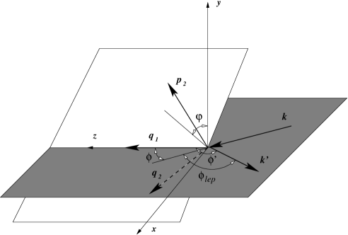
Figure 4: Kinematics of the generalized DVCS process in the target rest frame.

Instead of the kinematical variables ($\omega^{\prime}$, $E_{2}$, $\cos\phi^{\prime}$), it is more convenient to express the differential cross section in terms of the variables $\left(Q_{1}^{2},t,x_{B}\right)$, where $Q_{1}^{2}\equiv-q_{1}^{2}$. In the target rest frame, we have $Q_{1}^{2}=2M\omega yx_{B}$, where the invariant $y\equiv p_{1}\cdot q_{1}/p_{1}\cdot k=\left(\omega-\omega^{\prime}\right)/\omega$ and accordingly, Eq. (65) turns into:

$$\cos\phi_{2} = \frac{x_{B}M\left(1-t/Q_{1}^{2}\right)-t/\left(2M\right)}{\left|\vec{p}_{2}\right|\;\sqrt{1+4x_{B}^{2}M^{2}/Q_{1}^{2}}}\,\,.$$ (67)

Furthermore, from the conservation of three-momentum, $\vec{q}_{1}=\vec{k}-\vec{k}^{\prime}$, and writing the invariant $Q_{1}^{2}=-\left(k-k^{\prime}\right)^{2}=2\omega\omega^{\prime}\left(1-\cos\phi_{lep}\right)$, where $\phi_{lep}$ is the angle between the incident and scattered lepton momenta, we get for the polar angles of the incoming and scattered leptons:

$$\cos\phi = \frac{1+2yx_{B}^{2}M^{2}/Q_{1}^{2}}{\sqrt{1+4x_{B}^{2}M^{2}/Q_{1}^{2}}}$$ (68)

and

$$\cos\phi^{\prime} = \frac{1}{\sqrt{1+4x_{B}^{2}M^{2}/Q_{1}^{2}}}\left[1-\frac{2yx_{B}^{2}M^{2}}{\left(1-y\right)Q_{1}^{2}}\right]\,\,,$$ (69)

respectively. The differential cross section can then be written as:

$$\frac{d^{4}\sigma}{dx_{B}dQ_{1}^{2}dtd\varphi} = \frac{1}{32}\frac{1}{\left(2\pi\right)^{4}}\frac{x_{B}y^{2}}{Q_{1}^{4}}\frac{1}{\sqrt{1+4x_{B}^{2}M^{2}/Q_{1}^{2}}}\left|{\textrm{T}}\right|^{2}\,\,.$$ (70)

Finally, energy conservation, $M+\nu_{1}=E_{2}+\nu_{2}$, implies that the energy of the outgoing real photon in the target rest frame is $\nu_{2}=\left(Q_{1}^{2}+x_{B}t\right)/\left(2Mx_{B}\right)$. Alternatively, we can write the invariant momentum transfer as $t\equiv\left(q_{2}-q_{1}\right)^{2}=-Q_{1}^{2}-2\nu_{2}\left(\omega y-\sqrt{\omega^{2}y^{2}+Q_{1}^{2}}\;\cos\theta_{B\gamma}\right)$, where $\theta_{B\gamma}$ denotes the scattering angle between the incoming virtual weak boson and outgoing real photon. Combining both expressions gives:

$$\cos\theta_{B\gamma} = \frac{Q_{1}^{2}\nu_{2}+x_{B}M\left(Q_{1}^{2}+t\right)}{Q_{1}^{2}\nu_{2}\sqrt{1+4x_{B}^{2}M^{2}/Q_{1}^{2}}}\,\,,$$ (71)

or, on the other hand, the invariant $t$ can be expressed as a function of the angle $\theta_{B\gamma}$:

$$t = -Q_{1}^{2}\,\frac{1+\left(1-\sqrt{1+4x_{B}^{2}M^{2}/Q_{1}^{2}}\;\cos\theta_{B\gamma}\right)Q_{1}^{2}/\left(2x_{B}^{2}M^{2}\right)}{1+\left(1-\sqrt{1+4x_{B}^{2}M^{2}/Q_{1}^{2}}\;\cos\theta_{B\gamma}\right)Q_{1}^{2}/\left(2x_{B}M^{2}\right)}\,\,.$$ (72)

In the following, we determine the kinematically allowed region for the generalized DVCS process, which requires finding the upper and lower limits of the invariants $x_{B}$, $y$ and $t$. The kinematics are subject to the following constraints:

1. The energy of the incoming lepton beam is fixed at $\omega=20\;\mathrm{GeV}$.

2. The invariant mass squared of the virtual boson–nucleon system should be above the resonance region, $\hat{s}\equiv\left(p_{1}+q_{1}\right)^{2}\geq\hat{s}_{\rm min}=4\;\mathrm{GeV}^{2}$.

3. The virtuality of the incoming boson has to be large enough to ensure light-cone dominance of the scattering process, $Q_{1}^{2}\geq Q_{\rm 1min}^{2}=2.5\;\mathrm{GeV}^{2}$.

4. The momentum transfer squared should be as small as possible, e.g. $0.1\;\mathrm{GeV^{2}}\leq\left|t\right|\leq 0.2\;\mathrm{GeV^{2}}$, which yields a low-energy nucleon and a high-energy real photon with in the final state.

The constraint (2) leads to a lower limit on the variable $y$:

$$y_{\rm min} = \frac{\hat{s}_{\rm min}-M^{2}}{\left(s-M^{2}\right)\left(1-x_{B}\right)}\ .$$ (73)

On the other hand, when the incoming lepton is aligned along the $z$-axis, i.e. $\phi_{lep}=180^{\circ}$, the scaling variable $y$ reaches its maximum value:

$$y_{\rm max} = \left(1+\frac{M^{2}x_{B}}{s-M^{2}}\right)^{-1}\ .$$ (74)

The region in the $x_{B}y$ plane is then bounded by three curves, illustrated in Fig. 5. These are given by $y_{\rm min}$ in Eq. (73), $y_{\rm max}$ in Eq. (74), and $y=Q_{\rm 1min}^{2}/\left[\left(s-M^{2}\right)x_{B}\right]$, which follows from the constraint (3). Next, both the lower and upper limits of the invariant $t$ can be determined in the virtual weak boson–nucleon center of mass frame. Here the kinematic limits of $t$ are given by (up to relative corrections of the order $x_{B}M^{2}/Q_{1}^{2}$):

$$t_{\rm min}=\frac{-M^{2}x_{B}^{2}}{1-x_{B}\left(1-M^{2}/Q_{1}^{2}\right)} \mathrm{and} t_{\rm max}=\frac{M^{2}x_{B}^{2}-2M^{2}x_{B}+Q_{1}^{2}\left(x_{B}-1\right)/x_{B}}{1-x_{B}\left(1-M^{2}/Q_{1}^{2}\right)}\ ,$$ (75)

at the scattering angles of $0^{\circ}$ and $180^{\circ}$, respectively, between the initial and final nucleons.

Figure 5: Kinematics of the DVCS process: the dashed curve gives $y_{\rm min}$ in Eq. (73), the solid represents $y_{\rm max}$ in Eq. (74), and the dotted corresponds to $y=Q_{\rm 1min}^{2}/\left[\left(s-M^{2}\right)x_{B}\right]$. The region bounded by the three curves is that kinematically allowed for $\hat{s}\geq 4\;\mathrm{GeV}^{2}$ and $Q_{1}^{2}\geq 2.5\;\mathrm{GeV}^{2}$ with an $\omega=20\;\mathrm{GeV}$ lepton beam.

Finally, we select one kinematical point within the allowed region in the $x_{B}y$ plane, namely $Q_{1}^{2}=2.5\;\mathrm{GeV}^{2}$ and $x_{B}=0.35$. For this point, in Fig. 6 we plot the invariant momentum transfer against the scattering angle $\theta_{B\gamma}$, which varies between $-0.15\;\mathrm{GeV}^{2}$ and $-1.433\;\mathrm{GeV}^{2}$ for $0\leq\theta_{B\gamma}\leq 15^{\circ}$. We also set the angle between the lepton and nucleon scattering planes to $\varphi=0$. Then, with the so-called in-plane kinematics, the polar angles of both incoming and scattered leptons are fixed to $\phi=20.2^{\circ}$ and $\phi^{\prime}=25.3^{\circ}$, respectively.

Figure 6: Invariant momentum transfer squared as a function of the scattering angle between the incoming virtual weak boson and outgoing real photon in the target rest frame, for $Q_{1}^{2}=2.5\;\mathrm{GeV}^{2}$ and $x_{B}=0.35$.

III.2 Model

To proceed with a numerical study of the wDVCS process, we need a model of the OFPDs. Since this is an exploratory study, rather than a detailed one intended for comparison to experiment, we choose for simplicity a toy model to illustrate the main features of wDVCS and the differences with electromagnetic DVCS.

Inherent in our model are the following approximations:

• The sea quark contributions are negligible, which implies that the “plus” OFPDs coincide with the “minus” OFPDs. For that reason, $H_{f}\equiv H_{f}^{val}$ and $\widetilde{H}_{f}\equiv\widetilde{H}_{f}^{val}$ for quark flavor $f=u$ or $d$, and similarly for the $E_{f}$ and $\widetilde{E}_{f}$ distributions.

• The $t$ dependence can be factorized from the other two scaling variables ($x$ and $\xi$) for all distributions, and the dependence of the OFPDs on $t$ is characterized by the corresponding form factors.

• The $\xi$ dependence of OFPDs appears only in the $\widetilde{E}_{f}$ distribution.

The parametrization of the unpolarized quark OFPDs in the proton is taken from Ref. Guichon:1998xv :

$$H_{u}^{val}\left(x,\xi,t\right) = u_{p}^{val}\left(x\right)F_{1u}\left(t\right)/2\ ,$$ (76)

$$H_{d}^{val}\left(x,\xi,t\right) = d_{p}^{val}\left(x\right)F_{1d}\left(t\right)\ ,$$ (77)

$$E_{u}^{val}\left(x,\xi,t\right) = u_{p}^{val}\left(x\right)F_{2u}\left(t\right)/2\ ,$$ (78)

$$E_{d}^{val}\left(x,\xi,t\right) = d_{p}^{val}\left(x\right)F_{2d}\left(t\right)\ ,$$ (79)

where the unpolarized valence quark distributions are given by Radyushkin:1998rt :

$$u_{p}^{val}\left(x\right) = 1.89x^{-0.4}\left(1-x\right)^{3.5}\left(1+6x\right)\ ,$$ (80)

$$d_{p}^{val}\left(x\right) = 0.54x^{-0.6}\left(1-x\right)^{4.2}\left(1+8x\right)\ .$$ (81)

They closely reproduce the corresponding GRV parametrizations Gluck:1994uf at a low normalization point, $-q_{1}^{2}\simeq 1\;\mathrm{GeV}^{2}$ Musatov:1999gv . The $u$- and $d$-quark form factors in Eqs. (76)–(79) can be extracted from the proton and neutron Dirac and Pauli form factors, neglecting strangeness and heavier flavors, according to $F_{1p\left(n\right)}=Q_{u}F_{1u\left(d\right)}+Q_{d}F_{1d\left(u\right)}$ and $F_{2p\left(n\right)}=Q_{u}F_{2u\left(d\right)}+Q_{d}F_{2d\left(u\right)}$, which are in turn related to the Sachs electric and magnetic form factors:

$$F_{1p\left(n\right)}\left(t\right) = \left[G_{Ep\left(n\right)}\left(t\right)-\frac{t}{4M^{2}}G_{Mp\left(n\right)}\left(t\right)\right]\left(1-\frac{t}{4M^{2}}\right)^{-1},$$ (82)

$$F_{2p\left(n\right)}\left(t\right) = \left[G_{Mp\left(n\right)}\left(t\right)-G_{Ep\left(n\right)}\left(t\right)\right]\left(1-\frac{t}{4M^{2}}\right)^{-1}.$$ (83)

At small $t$, both the proton and neutron magnetic form factors, as well as the proton electric form factor, are approximated by dipole fits, while the electric neutron form factor is taken to be zero:

$$G_{Ep}\left(t\right)=\frac{G_{Mp}\left(t\right)}{1+\kappa_{p}}=\frac{G_{Mn}\left(t\right)}{\kappa_{n}}=\left(1-\frac{t}{\Lambda^{2}}\right)^{-2}, \mathrm{and} G_{En}\left(t\right)=0\ ,$$ (84)

where $\kappa_{p}=1.793$ and $\kappa_{n}=-1.913$ are the proton and neutron anomalous magnetic moments, respectively, and the parameter $\Lambda^{2}=0.71\;\mathrm{GeV}^{2}$.

In the polarized case, we take for the valence distributions the factorized ansatz from Ref. Belitsky:2001ns :

$$\widetilde{H}_{u}^{val}\left(x,\xi,t\right) = \Delta u_{p}^{val}\left(x\right)\left(1-\frac{t}{m_{A}^{2}}\right)^{-2}\ ,$$ (85)

$$\widetilde{H}_{d}^{val}\left(x,\xi,t\right) = \Delta d_{p}^{val}\left(x\right)\left(1-\frac{t}{m_{A}^{2}}\right)^{-2}\ ,$$ (86)

where the mass $m_{A}=1.03\;\mathrm{GeV}$. The polarized valence quark distributions in the proton can be expressed in terms of the unpolarized distributions using a parameterization motivated by the SU(6) quark model Carlitz:1976in ; Goshtasbpour:1995eh :

$$\Delta u_{p}^{val} = \cos\theta_{D}\left(u_{p}^{val}-\frac{2}{3}d_{p}^{val}\right)\ ,$$ (87)

$$\Delta d_{p}^{val} = \cos\theta_{D}\left(-\frac{1}{3}d_{p}^{val}\right)\ ,$$ (88)

where $\cos\theta_{D}=\left[1+0.06\left(1-x^{2}\right)/\sqrt{x}\;\right]^{-1}$. Finally, for the $\widetilde{E}_{f}$ distribution we use an ansatz in which the distribution is dominated by the pion pole:

$$\widetilde{E}_{u}^{val}\left(x,\xi,t\right) = \frac{1}{2}F_{\pi}\left(t\right)\frac{\theta\left(\left|x\right|<\xi\right)}{2\xi}\;\phi_{\pi}\left(\frac{x+\xi}{2\xi}\right)\ ,$$ (89)

$$\widetilde{E}_{d}^{val}\left(x,\xi,t\right) = -\widetilde{E}_{u}^{val}\left(x,\xi,t\right)\ .$$ (90)

The function $F_{\pi}\left(t\right)$ is assumed to have a form valid for $-t\ll M^{2}$ Penttinen:1999th :

$$F_{\pi}\left(t\right) = \frac{4g_{A}M^{2}}{\left(m_{\pi}^{2}-t\right)}\left[1-\frac{1.7\left(m_{\pi}^{2}-t\right)/\mathrm{GeV^{2}}}{\left(1-t/2\;\mathrm{GeV^{2}}\right)^{2}}\right],$$ (91)

where $m_{\pi}\simeq 0.14\;\mathrm{GeV}$, and the axial charge of the nucleon is $g_{A}\simeq 1.267$. For the pion distribution amplitude in Eq. (90) we choose, for simplicity, its asymptotic form:

$$\phi_{\pi}\left(u\right) = 6u\left(1-u\right)\ .$$ (92)

Having defined the kinematics and described the model for the nucleon OFPDs, in the rest of this section we examine several specific DVCS processes.

III.3 Weak neutral current scattering

In this subsection we discuss two examples of the weak neutral current scattering process, for neutrino–proton and electron–proton scattering. For the case of an unpolarized neutron target, one can use isospin symmetry to express the neutron OFPDs in terms of proton OFPDs. To make our comparisons meaningful, in all cases the relevant unpolarized differential cross sections (70) will be plotted as a function of the angle $\theta_{B\gamma}$ for the same kinematical point, namely, $Q_{1}^{2}=2.5\;\mathrm{GeV}^{2}$ and $x_{B}=0.35$, with a lepton beam energy $\omega=20\;\mathrm{GeV}$.

III.3.1 Neutrino–proton scattering

Since neutrinos do not interact with photons, neutrino scattering from a proton via the exchange of a $Z^{0}$ boson measures the pure Compton contribution, with no contribution from the Bethe-Heitler process. The T-matrix for this process,

$$i\mathrm{T}_{\nu p} = \bar{u}\left(k^{\prime}\right)\left(\frac{-ig}{\cos\theta_{W}}\right)\gamma^{\lambda}\left(\frac{c_{V}^{\nu}-\gamma_{5}c_{A}^{\nu}}{2}\right)u\left(k\right)\left[\frac{-i\left(g_{\nu\lambda}-q_{1\nu}q_{1\lambda}/M_{Z^{0}}^{2}\right)}{q_{1}^{2}-M_{Z^{0}}^{2}}\right]\left(\frac{-\left|e\right|g}{\cos\theta_{W}}\right)\epsilon_{\mu}^{*}\left(q_{2}\right)\left(-i\mathcal{T}_{WN}^{\mu\nu}\right)\ ,$$ (93)

is then solely given by the DVCS diagram, Fig. 3(a). The vector and axial vector couplings at the $\nu\nu Z^{0}$ vertex are $c_{V}^{\nu}=c_{A}^{\nu}=1/2$. By taking into account that $M_{Z^{0}}^{2}\gg Q_{1}^{2}$ and $\cos\theta_{W}\equiv M_{W}/M_{Z^{0}}$, and further recalling that $g^{2}/\left(8M_{W}^{2}\right)\equiv G_{F}/\sqrt{2}$, where $G_{F}\simeq 1.166\cdot 10^{-5}\;\mathrm{GeV}^{-2}$ is the Fermi coupling constant, we arrive at:

$$\mathrm{T}_{\nu p} = \sqrt{2}\left|e\right|G_{F}\bar{u}\left(k^{\prime}\right)\gamma_{\nu}\left(1-\gamma_{5}\right)u(k)\epsilon_{\mu}^{*}\left(q_{2}\right)\mathcal{T}_{WN}^{\mu\nu}\ .$$ (94)

To compute the unpolarized cross section, one should average the square of the amplitude $\mathrm{T}_{\nu p}$ over the spins of the initial particles, and further sum it over the spins and polarizations of the final particles. In particular, the summation over the photon polarizations is performed using the Feynman gauge prescription, i.e. one can replace

$$\sum_{\gamma\;polar.}\epsilon_{\mu}^{*}\left(q_{2}\right)\epsilon_{\alpha}\left(q_{2}\right) \longrightarrow -g_{\mu\alpha}$$ (95)

by virtue of the Ward identity. As a result, we then write the spin-averaged square of the T-matrix in terms of factorized neutrino and weak neutral hadronic tensors,

$$\overline{\left|\mathrm{T}_{\nu p}\right|^{2}} = 8\pi\alpha G_{F}^{2}\ L_{\nu\beta}^{\left(\nu\right)}H_{WN}^{\nu\beta}\ ,$$ (96)

where $\alpha\equiv e^{2}/\left(4\pi\right)\simeq 1/137$ is the electromagnetic fine structure constant. The neutrino tensor $L_{\nu\beta}^{\left(\nu\right)}$ is given by:

$$L_{\nu\beta}^{\left(\nu\right)} = 8\left[k_{\nu}k^{\prime}_{\beta}+k_{\beta}k^{\prime}_{\nu}-g_{\nu\beta}\left(k\cdot k^{\prime}\right)-i\epsilon_{\nu\beta\sigma\tau}k^{\sigma}k^{\prime\tau}\right]\ .$$ (97)

The weak neutral hadronic tensor $H_{WN}^{\nu\beta}$, on the other hand, has a considerably more complicated structure. In the DVCS kinematics, however, in which $\mathcal{O}\left(t/q_{1}^{2}\right)$ and $\mathcal{O}\left(M^{2}/q_{1}^{2}\right)$ terms are neglected, and using the Feynman gauge prescription, this reduces to:

$$H_{WN}^{\nu\beta} = -\frac{1}{2}\mathcal{T}_{WN}^{\mu\nu}\left(\mathcal{T}_{\mu WN}^{\beta}\right)^{*}$$

$$= -\frac{1}{4}\left\{\mathcal{C}_{1WN}\left[g^{\nu\beta}-\frac{1}{\left(p\cdot q_{2}\right)}\left(p^{\nu}q_{2}^{\beta}+p^{\beta}q_{2}^{\nu}\right)+\frac{M^{2}}{\left(p\cdot q_{2}\right)^{2}}\left(1-\frac{t}{4M^{2}}\right)q_{2}^{\nu}q_{2}^{\beta}\right]-\mathcal{C}_{2WN}\frac{1}{\left(p\cdot q_{2}\right)}i\epsilon^{\nu\beta\delta\lambda}p_{\delta}q_{2\lambda}\right\}\ ,$$

where the functions $\mathcal{C}_{1WN}$ and $\mathcal{C}_{2WN}$ are given by:

$$\mathcal{C}_{1WN} = \left(1-\xi^{2}\right)\left(\left|\mathcal{H}_{WN}^{+}\right|^{2}+\left|\mathcal{H}_{WN}^{-}\right|^{2}+\left|\widetilde{\mathcal{H}}_{WN}^{+}\right|^{2}+\left|\widetilde{\mathcal{H}}_{WN}^{-}\right|^{2}\right)-\left(\xi^{2}+\frac{t}{4M^{2}}\right)\left(\left|\mathcal{E}_{WN}^{+}\right|^{2}+\left|\mathcal{E}_{WN}^{-}\right|^{2}\right)$$ (99)

$$\hskip 14.22636pt-\xi^{2}\frac{t}{4M^{2}}\left(\left|\widetilde{\mathcal{E}}_{WN}^{+}\right|^{2}+\left|\widetilde{\mathcal{E}}_{WN}^{-}\right|^{2}\right)-2\xi^{2}\Re\left(\mathcal{H}_{WN}^{+*}\mathcal{E}_{WN}^{+}+\mathcal{H}_{WN}^{-*}\mathcal{E}_{WN}^{-}+\widetilde{\mathcal{H}}_{WN}^{+*}\widetilde{\mathcal{E}}_{WN}^{+}+\widetilde{\mathcal{H}}_{WN}^{-*}\widetilde{\mathcal{E}}_{WN}^{-}\right),$$

$$\mathcal{C}_{2WN} = -2\left[\left(1-\xi^{2}\right)\Re\left(\mathcal{H}_{WN}^{+*}\mathcal{H}_{WN}^{-}+\widetilde{\mathcal{H}}_{WN}^{+*}\widetilde{\mathcal{H}}_{WN}^{-}\right)-\left(\xi^{2}+\frac{t}{4M^{2}}\right)\Re\left(\mathcal{E}_{WN}^{+*}\mathcal{E}_{WN}^{-}\right)-\xi^{2}\frac{t}{4M^{2}}\Re\left(\widetilde{\mathcal{E}}_{WN}^{+*}\widetilde{\mathcal{E}}_{WN}^{-}\right)\right.$$ (100)

$$\hskip 14.22636pt\left.-\xi^{2}\Re\left(\mathcal{H}_{WN}^{+*}\mathcal{E}_{WN}^{-}+\mathcal{E}_{WN}^{+*}\mathcal{H}_{WN}^{-}+\widetilde{\mathcal{H}}_{WN}^{+*}\widetilde{\mathcal{E}}_{WN}^{-}+\widetilde{\mathcal{E}}_{WN}^{+*}\widetilde{\mathcal{H}}_{WN}^{-}\right)\right].$$

The result of the contraction of the tensor $H_{WN}^{\nu\beta}$ with $L_{\nu\beta}^{\left(\nu\right)}$ in Eq. (97) can be presented in a compact form as:

$$\overline{\left|\mathrm{T}_{\nu p}\right|^{2}} = \frac{16\pi\alpha G_{F}^{2}Q_{1}^{2}}{y^{2}}\left\{\left[1+\left(1-y\right)^{2}\right]\mathcal{C}_{1WN}-\left[1-\left(1-y\right)^{2}\right]\mathcal{C}_{2WN}\right\}.$$ (101)

III.3.2 Electron–proton scattering

Unlike in the neutrino case, for electron scattering both the Compton and Bethe-Heitler processes contribute, in which case the $ep$ amplitude is given by the sum $\mathrm{T}_{ep}=\mathrm{T}_{Cep}+\mathrm{T}_{BHep}$. By replacing neutrinos with electrons in Eq. (93), we can immediately write for the Compton part of the T-matrix:

$$\mathrm{T}_{Cep} = 2\sqrt{2}\left|e\right|G_{F}\bar{u}\left(k^{\prime}\right)\gamma_{\nu}\left(c_{V}^{e}-\gamma_{5}c_{A}^{e}\right)u(k)\epsilon_{\mu}^{*}\left(q_{2}\right)\mathcal{T}_{WN}^{\mu\nu}\ ,$$ (102)

where the couplings are now $c_{V}^{e}=-1/2+2\sin^{2}\theta_{W}$ and $c_{A}^{e}=-1/2$. The spin-averaged square of $\mathrm{T}_{Cep}$ then reads:

$$\overline{\left|\mathrm{T}_{Cep}\right|^{2}} = 32\pi\alpha G_{F}^{2}\ L_{\nu\beta}^{\left(e\right)}H_{WN}^{\nu\beta}\ .$$ (103)

The hadronic tensor $H_{WN}^{\nu\beta}$ is the same as in Eq. (LABEL:eq:hadronictensorWN), while the electron tensor has an additional factor of $1/2$ from averaging over the initial electron spins:

$$L_{\nu\beta}^{\left(e\right)} = 2\left\{\left[\left(c_{V}^{e}\right)^{2}+\left(c_{A}^{e}\right)^{2}\right]\left[k_{\nu}k^{\prime}_{\beta}+k_{\beta}k^{\prime}_{\nu}-g_{\nu\beta}\left(k\cdot k^{\prime}\right)\right]-2c_{V}^{e}c_{A}^{e}i\epsilon_{\nu\beta\sigma\tau}k^{\sigma}k^{\prime\tau}\right\}\ ,$$ (104)

and hence

$$\overline{\left|\mathrm{T}_{Cep}\right|^{2}} = \frac{16\pi\alpha G_{F}^{2}Q_{1}^{2}}{y^{2}}\left\{\left[\left(c_{V}^{e}\right)^{2}+\left(c_{A}^{e}\right)^{2}\right]\left[1+\left(1-y\right)^{2}\right]\mathcal{C}_{1WN}-2c_{V}^{e}c_{A}^{e}\left[1-\left(1-y\right)^{2}\right]\mathcal{C}_{2WN}\right\}.$$ (105)

For the Bethe-Heitler contribution, since both the initial and final leptons are electrons, both diagrams (b) and (c) in Fig. 3 contribute. The full Bethe-Heitler amplitude is given by:

$$\mathrm{T}_{BHep} = 2\sqrt{2}\left|e\right|G_{F}\epsilon_{\mu}^{*}\left(q_{2}\right)\bar{u}\left(k^{\prime}\right)\left[\frac{\gamma^{\mu}\left(\not\!k^{\prime}+\not\!q_{2}\right)\gamma^{\nu}\left(c_{V}^{e}-\gamma_{5}c_{A}^{e}\right)}{\left(k^{\prime}+q_{2}\right)^{2}}+\frac{\gamma^{\nu}\left(c_{V}^{e}-\gamma_{5}c_{A}^{e}\right)\left(\not\!k-\not\!q_{2}\right)\gamma^{\mu}}{\left(k-q_{2}\right)^{2}}\right]u\left(k\right)$$ (106)

$$\times\left\langle p\left(p_{2},s_{2}\right)\right|J_{\nu}^{NC}\left(0\right)\left|p\left(p_{1},s_{1}\right)\right\rangle\ .$$

Accordingly, the electron and hadronic tensors in the Bethe-Heitler amplitude

$$\overline{\left|\mathrm{T}_{BHep}\right|^{2}} = 32\pi\alpha G_{F}^{2}\ L_{BH}^{\nu\beta}H_{\nu\beta}^{BH}$$ (107)

are given by:

$$L_{BH}^{\nu\beta} = -\frac{1}{2}\mathrm{Tr}\left\{\not\!k^{\prime}\left[\frac{\left(\gamma^{\mu}\not\!q_{2}+2k^{\prime\mu}\right)\gamma^{\nu}\left(c_{V}^{e}-\gamma_{5}c_{A}^{e}\right)}{2\left(k^{\prime}\cdot q_{2}\right)}+\frac{\gamma^{\nu}\left(c_{V}^{e}-\gamma_{5}c_{A}^{e}\right)\left(\not\!q_{2}\gamma^{\mu}-2k^{\mu}\right)}{2\left(k\cdot q_{2}\right)}\right]\right.$$ (108)

$$\hskip 14.22636pt\left.\times\not\!k\left[\frac{\gamma^{\beta}\left(c_{V}^{e}-\gamma_{5}c_{A}^{e}\right)\left(\not\!q_{2}\gamma_{\mu}+2k^{\prime}_{\mu}\right)}{2\left(k^{\prime}\cdot q_{2}\right)}+\frac{\left(\gamma_{\mu}\not\!q_{2}-2k_{\mu}\right)\gamma^{\beta}\left(c_{V}^{e}-\gamma_{5}c_{A}^{e}\right)}{2\left(k\cdot q_{2}\right)}\right]\right\}$$

$$= \frac{2}{\left(k^{\prime}\cdot q_{2}\right)}\left\{\left[\left(c_{V}^{e}\right)^{2}+\left(c_{A}^{e}\right)^{2}\right]\left[k^{\nu}q_{2}^{\beta}+k^{\beta}q_{2}^{\nu}-g^{\nu\beta}\left(k\cdot q_{2}\right)\right]-2c_{V}^{e}c_{A}^{e}i\epsilon^{\nu\beta\sigma\tau}k_{\sigma}q{}_{2\tau}\right\}$$

$$+\frac{2}{\left(k\cdot q_{2}\right)}\left\{\left[\left(c_{V}^{e}\right)^{2}+\left(c_{A}^{e}\right)^{2}\right]\left[k^{\prime\nu}q_{2}^{\beta}+k^{\prime\beta}q_{2}^{\nu}-g^{\nu\beta}\left(k^{\prime}\cdot q_{2}\right)\right]+2c_{V}^{e}c_{A}^{e}i\epsilon^{\nu\beta\sigma\tau}k^{\prime}_{\sigma}q{}_{2\tau}\right\}$$

$$+\frac{2}{\left(k^{\prime}\cdot q_{2}\right)\left(k\cdot q_{2}\right)}\left\{\left[\left(c_{V}^{e}\right)^{2}+\left(c_{A}^{e}\right)^{2}\right]\left[\left(k\cdot q_{2}\right)\left[k^{\nu}k^{\prime\beta}+k^{\beta}k^{\prime\nu}+2k^{\prime\nu}k^{\prime\beta}\right]-\left(k^{\prime}\cdot q_{2}\right)\left[k^{\nu}k^{\prime\beta}+k^{\beta}k^{\prime\nu}+2k^{\nu}k^{\beta}\right]\right.\right.$$

$$\hskip 14.22636pt\left.+\left(k\cdot k^{\prime}\right)\left[k^{\nu}q_{2}^{\beta}+k^{\beta}q_{2}^{\nu}-k^{\prime\nu}q_{2}^{\beta}-k^{\prime\beta}q_{2}^{\nu}+2k^{\nu}k^{\prime\beta}+2k^{\beta}k^{\prime\nu}\right]+2g^{\nu\beta}\left(k\cdot k^{\prime}\right)\left[\left(k^{\prime}\cdot q_{2}\right)-\left(k\cdot q_{2}\right)-\left(k\cdot k^{\prime}\right)\right]\right]$$

$$\hskip 14.22636pt-2c_{V}^{e}c_{A}^{e}i\epsilon^{\nu\beta\sigma\tau}\left[\left(k\cdot k^{\prime}\right)\left[2k{}_{\sigma}k^{\prime}{}_{\tau}+k{}_{\sigma}q{}_{2\tau}+k^{\prime}{}_{\sigma}q{}_{2\tau}\right]+\left[\left(k\cdot q_{2}\right)-\left(k^{\prime}\cdot q_{2}\right)\right]k{}_{\sigma}k^{\prime}{}_{\tau}\right]\bigg{\}}$$

and

$$H_{\nu\beta}^{BH} = \frac{1}{2}\sum_{s_{1},s_{2}}\left\langle p\left(p_{2},s_{2}\right)\right|J_{\nu}^{NC}\left(0\right)\left|p\left(p_{1},s_{1}\right)\right\rangle\left\langle p\left(p_{2},s_{2}\right)\right|J_{\beta}^{NC}\left(0\right)\left|p\left(p_{1},s_{1}\right)\right\rangle^{*}\ ,$$ (109)

respectively. The weak neutral transition current $J_{\nu}^{NC}$ in Eq. (109) consists of vector and axial vector parts:

$$J_{\nu}^{NC}\left(0\right) = \frac{1}{2}\left[V_{\nu}^{NC}\left(0\right)-A_{\nu}^{NC}\left(0\right)\right]$$ (110)

$$= \frac{1}{2}\sum_{f}\left[c_{V}^{f}\bar{\psi}_{f}\left(0\right)\gamma_{\nu}\psi_{f}\left(0\right)-c_{A}^{f}\bar{\psi}_{f}\left(0\right)\gamma_{\nu}\gamma_{5}\psi_{f}\left(0\right)\right]\ .$$

Their matrix elements are parametrized as (see e.g. Ref. Thomas:2001kw ):

$$\left\langle p\left(p_{2},s_{2}\right)\right|V_{\nu}^{NC}\left(0\right)\left|p\left(p_{1},s_{1}\right)\right\rangle = \bar{u}\left(p_{2},s_{2}\right)\left[F_{1}^{NC}\left(t\right)\gamma_{\nu}-F_{2}^{NC}\left(t\right)\frac{i\sigma_{\nu\lambda}r^{\lambda}}{2M}\right]u\left(p_{1},s_{1}\right)\ ,$$ (111)

$$\left\langle p\left(p_{2},s_{2}\right)\right|A_{\nu}^{NC}\left(0\right)\left|p\left(p_{1},s_{1}\right)\right\rangle = \bar{u}\left(p_{2},s_{2}\right)\left[G_{A}^{NC}\left(t\right)\gamma_{\nu}\gamma_{5}-G_{P}^{NC}\left(t\right)\frac{\gamma_{5}r_{\nu}}{2M}\right]u\left(p_{1},s_{1}\right)\ ,$$ (112)

which then gives the following expression for the hadronic tensor:

$$H_{\nu\beta}^{BH} = \frac{1}{4}\left\{t\left[g_{\nu\beta}-\frac{r_{\nu}r_{\beta}}{t}\right]\left[F_{1}^{NC}\left(t\right)+F_{2}^{NC}\left(t\right)\right]^{2}+4\left[p_{1\nu}-\frac{r_{\nu}}{2}\right]\left[p_{1\beta}-\frac{r_{\beta}}{2}\right]\left[\left(F_{1}^{NC}\left(t\right)\right)^{2}-\frac{t}{4M^{2}}\left(F_{2}^{NC}\left(t\right)\right)^{2}\right]\right\}$$ (113)

$$+\left[\left(p_{1\nu}-\frac{r_{\nu}}{2}\right)\left(p_{1\beta}-\frac{r_{\beta}}{2}\right)-M^{2}\left(1-\frac{t}{4M^{2}}\right)g_{\nu\beta}\right]\left(G_{A}^{NC}\left(t\right)\right)^{2}+\frac{r_{\nu}r_{\beta}}{4}\left(1-\frac{t}{4M^{2}}\right)\left(G_{P}^{NC}\left(t\right)\right)^{2}$$

$$-\frac{r_{\nu}r_{\beta}}{4}\left[G_{A}^{NC}\left(t\right)+G_{P}^{NC}\left(t\right)\right]^{2}-i\epsilon_{\nu\beta\sigma\tau}p_{1}^{\sigma}p_{2}^{\tau}\left[F_{1}^{NC}\left(t\right)+F_{2}^{NC}\left(t\right)\right]G_{A}^{NC}\left(t\right)\ .$$

We express the result of the contraction of Eq. (113) with the leptonic tensor in Eq. (108) in terms of the kinematical invariants $x_{B}$, $y$, $Q_{1}^{2}$ and $t$, and the scalar product:

$$k\cdot q_{2} = \omega\nu_{2}\left[1-\left(\sin\phi\sin\theta_{B\gamma}+\cos\phi\cos\theta_{B\gamma}\right)\right]$$ (114)

$$= Q_{1}^{2}\left.\frac{1+x_{B}t/Q_{1}^{2}}{y\left(1+4x_{B}^{2}M^{2}/Q_{1}^{2}\right)}\right\{1-\frac{y}{2}-\frac{1}{2}\left(1+\frac{2yx_{B}^{2}M^{2}}{Q_{1}^{2}}\right)\left(\frac{1+t/Q_{1}^{2}}{1+x_{B}t/Q_{1}^{2}}\right)$$

$$\left.-\sqrt{\left(1-y-\frac{y^{2}x_{B}^{2}M^{2}}{Q_{1}^{2}}\right)\left[1-\frac{1+t/Q_{1}^{2}}{1+x_{B}t/Q_{1}^{2}}-\frac{x_{B}^{2}M^{2}}{Q_{1}^{2}}\left(\frac{1+t/Q_{1}^{2}}{1+x_{B}t/Q_{1}^{2}}\right)^{2}\right]}\;\right\}.$$

Moreover, it is convenient to introduce the dimensionless variables $\tau\equiv t/Q_{1}^{2}$, $\mu\equiv M^{2}/Q_{1}^{2}$ and $\kappa\equiv\left(k\cdot q_{2}\right)/Q_{1}^{2}$. The latter can be written in the following form:

$$\kappa = \frac{1}{2y\left(1+4x_{B}^{2}\mu\right)}\left\{1-2\mathcal{K}-\tau\left[1-x_{B}\left(2-y\right)+2x_{B}^{2}y\mu\right]+2x_{B}^{2}y\mu\right\}-\frac{1}{2}\ ,$$ (115)

where

$$\mathcal{K} = \sqrt{-\left(1-y-x_{B}^{2}y^{2}\mu\right)\left[\left(1-x_{B}\right)\tau+x_{B}\left(1-x_{B}\right)\tau^{2}+x_{B}^{2}y^{2}\mu\left(1+\tau\right)^{2}\right]}$$ (116)

is the $1/\sqrt{Q_{1}^{2}}$-power suppressed kinematical factor. In terms of these variables, the Bethe-Heitler squared amplitude can then be written:

$$\overline{\left|\mathrm{T}_{BHep}\right|^{2}} = -32\pi\alpha G_{F}^{2}Q_{1}^{2}\left[\frac{1}{2\kappa\left(2\kappa+\tau+1\right)x_{B}^{2}y^{2}}\right]$$ (117)

$$\times\Bigg{\{}\left[\left(c_{V}^{e}\right)^{2}+\left(c_{A}^{e}\right)^{2}\right]\left[x_{B}^{2}y^{2}\tau\left[\left(2\kappa+1\right)^{2}+\left(2\kappa+\tau\right)^{2}\right]\left[F_{1}^{NC}\left(t\right)+F_{2}^{NC}\left(t\right)\right]^{2}\right.$$

$$+2\left[2\tau\left(1-y\right)-x_{B}y\tau\left(4\kappa+\tau+1\right)+y^{2}\left[\tau+x_{B}\tau\left(2\kappa+\tau\right)+x_{B}^{2}\mu\left[1+8\kappa^{2}+\tau^{2}+4\kappa\left(1+\tau\right)\right]\right]\right]$$

$$\left.\times\left[\left(F_{1}^{NC}\left(t\right)\right)^{2}-\frac{t}{4M^{2}}\left(F_{2}^{NC}\left(t\right)\right)^{2}\right]\right]$$

$$+\left[4\tau-2y\tau\left[2+x_{B}\left(4\kappa+\tau+1\right)\right]+y^{2}\left[2\tau+2x_{B}\tau\left(2\kappa+\tau\right)+x_{B}^{2}\left(\tau-2\mu\right)\left[1+8\kappa^{2}+\tau^{2}+4\kappa\left(1+\tau\right)\right]\right]\right]$$

$$\times\left[\left(c_{V}^{e}\right)^{2}+\left(c_{A}^{e}\right)^{2}\right]\left(G_{A}^{NC}\left(t\right)\right)^{2}$$

$$+4x_{B}y\tau\left[2\left(1-\tau\right)+y\left[2\left(2\kappa+\tau\right)-x_{B}\left(1-\tau\right)\left(4\kappa+\tau+1\right)\right]\right]c_{V}^{e}c_{A}^{e}\left[F_{1}^{NC}\left(t\right)+F_{2}^{NC}\left(t\right)\right]G_{A}^{NC}\left(t\right)\Bigg{\}},$$

where the term $1/\left[2\kappa\left(2\kappa+\tau+1\right)\right]$ comes from the lepton propagators. Note that, in contrast to the Compton contribution, Eq. (117) is the result of the exact calculation. Each of the vector form factors can be further decomposed into linear combinations of flavor triplet, octet and singlet form factors:

$$F_{1\left(2\right)}^{NC}\left(t\right) = \left(1-2\sin^{2}\theta_{W}\right)\left[F_{1\left(2\right)}^{3}\left(t\right)+\frac{1}{6}F_{1\left(2\right)}^{8}\left(t\right)\right]-\frac{1}{6}F_{1\left(2\right)}^{0}\left(t\right)\ ,$$ (118)

while the axial and pseudoscalar form factors can be written, in general, as differences between the isovector and strangeness form factors:

$$G_{A\left(P\right)}^{NC}\left(t\right) = G_{A\left(P\right)}^{3}\left(t\right)-\frac{1}{2}G_{A\left(P\right)}^{s}\left(t\right)\ .$$ (119)

If one further neglects sea quark contributions, then these form factors can be written as:

$$F_{1\left(2\right)}^{3}\left(t\right) = \frac{1}{2}\left[F_{1\left(2\right)u}\left(t\right)-F_{1\left(2\right)d}\left(t\right)\right]\ ,$$ (120)

$$F_{1\left(2\right)}^{8}\left(t\right)=F_{1\left(2\right)}^{0}\left(t\right) = \left[F_{1\left(2\right)u}\left(t\right)+F_{1\left(2\right)d}\left(t\right)\right]\ ,$$ (121)

$$G_{A\left(P\right)}^{NC}\left(t\right) = G_{A\left(P\right)}^{3}\left(t\right).$$ (122)

Recall that the $t$ dependence of the $u$- and $d$-quark form factors is given by the Dirac and Pauli form factors, whereas for the axial and pseudoscalar form factors we use the parametrizations:

$$G_{A}^{NC}\left(t\right) = \frac{g_{A}}{2}\left(1-\frac{t}{m_{A}^{2}}\right)^{-2}\ ,$$ (123)

$$G_{P}^{NC}\left(t\right) = \frac{G_{A}^{NC}\left(t\right)}{2}\left(\frac{4M^{2}}{m_{\pi}^{2}-t}\ \right).$$ (124)

The interference terms between the Compton and Bethe-Heitler contributions,

$$\mathcal{I}_{ep} = \mathrm{T}_{Cep}\mathrm{T}_{BHep}^{*}+\mathrm{T}_{Cep}^{*}\mathrm{T}{}_{BHep}\ ,$$ (125)

are particularly interesting, since they are linear in the integrals of OFPDs. Substituting the expressions in Eqs. (102) and (106) into Eq. (125), and averaging and summing over the initial and final spins, respectively, the interference term can be written in terms of the electron and hadronic traces as:

$$\mathcal{I}_{ep} = -4\pi\alpha G_{F}^{2}\left\{\mathrm{Tr}\left\{\not\!k^{\prime}\gamma_{\nu}\left(c_{V}^{e}-\gamma_{5}c_{A}^{e}\right)\not\!k\left[\frac{\gamma^{\beta}\left(c_{V}^{e}-\gamma_{5}c_{A}^{e}\right)\left(\not\!q_{2}\gamma_{\mu}+2k^{\prime}_{\mu}\right)}{2\left(k^{\prime}\cdot q_{2}\right)}+\frac{\left(\gamma_{\mu}\not\!q_{2}-2k_{\mu}\right)\gamma^{\beta}\left(c_{V}^{e}-\gamma_{5}c_{A}^{e}\right)}{2\left(k\cdot q_{2}\right)}\right]\right\}\right.$$

$$\times\mathrm{Tr}\left\{\left(\not\!p_{2}+M\right)\hat{\mathcal{T}}_{WN}^{\mu\nu}\left(\not\!p_{1}+M\right)\left[F_{1}^{NC}\left(t\right)\gamma_{\beta}+F_{2}^{NC}\left(t\right)\frac{i\sigma_{\beta\tau}r^{\tau}}{2M}-G_{A}^{NC}\left(t\right)\gamma_{\beta}\gamma_{5}-G_{P}^{NC}\left(t\right)\frac{\gamma_{5}r_{\beta}}{2M}\right]\right\}$$

$$+\mathrm{Tr}\left\{\not\!k\gamma_{\beta}\left(c_{V}^{e}-\gamma_{5}c_{A}^{e}\right)\not\!k^{\prime}\left[\frac{\left(\gamma^{\mu}\not\!q_{2}+2k^{\prime\mu}\right)\gamma^{\nu}\left(c_{V}^{e}-\gamma_{5}c_{A}^{e}\right)}{2\left(k^{\prime}\cdot q_{2}\right)}+\frac{\gamma^{\nu}\left(c_{V}^{e}-\gamma_{5}c_{A}^{e}\right)\left(\not\!q_{2}\gamma^{\mu}-2k^{\mu}\right)}{2\left(k\cdot q_{2}\right)}\right]\right\}$$

$$\left.\times\mathrm{Tr}\left\{\left(\not\!p_{1}+M\right)\left(\hat{\mathcal{T}}_{\mu WN}^{\beta}\right)^{*}\left(\not\!p_{2}+M\right)\left[F_{1}^{NC}\left(t\right)\gamma_{\nu}-F_{2}^{NC}\left(t\right)\frac{i\sigma_{\nu\lambda}r^{\lambda}}{2M}-G_{A}^{NC}\left(t\right)\gamma_{\nu}\gamma_{5}+G_{P}^{NC}\left(t\right)\frac{\gamma_{5}r_{\nu}}{2M}\right]\right\}\right\}\ ,$$

where the amplitude ${\hat{\mathcal{T}}}_{WN}^{\mu\nu}$ is the spinorless part of the reduced virtual Compton scattering amplitude $\mathcal{T}_{WN}^{\mu\nu}$:

$$\mathbf{\mathcal{T}}_{WN}^{\mu\nu} = \bar{u}\left(p_{2},s_{2}\right){\hat{\mathcal{T}}}_{WN}^{\mu\nu}u\left(p_{1},s_{1}\right).$$ (127)

To be consistent, we need to keep the same level of accuracy as in the Compton part, i.e. we should neglect terms that are of $\mathcal{O}\left(t/q_{1}^{2}\right)$ and $\mathcal{O}\left(M^{2}/q_{1}^{2}\right)$ order. Accordingly, the variable $\kappa$ becomes $\kappa=\left[\left(1-y\right)-2\mathcal{K}\right]/\left(2y\right)$. Furthermore, we should only keep terms linear in $\mathcal{K}$. After the contraction, we obtain:

$$\mathcal{I}_{ep} = -16\pi\alpha G_{F}^{2}Q_{1}^{2}\left[\frac{1}{2\kappa\left(2\kappa+\tau+1\right)x_{B}y^{3}}\right]\left\{\left[\left(c_{V}^{e}\right)^{2}+\left(c_{A}^{e}\right)^{2}\right]\left[4\mathcal{K}\left(2-2y+y^{2}\right)\right]\right.$$ (128)

$$\times\left[F_{1}^{NC}\left(t\right)\Re\left(\mathcal{H}_{WN}^{+}\right)-\frac{t}{4M^{2}}F_{2}^{NC}\left(t\right)\Re\left(\mathcal{E}_{WN}^{+}\right)+G_{A}^{NC}\left(t\right)\Re\left(\widetilde{\mathcal{H}}_{WN}^{-}\right)\right.$$

$$\left.+\xi\left[\left[F_{1}^{NC}\left(t\right)+F_{2}^{NC}\left(t\right)\right]\Re\left(\widetilde{\mathcal{H}}_{WN}^{+}\right)+G_{A}^{NC}\left(t\right)\left[\Re\left(\mathcal{H}_{WN}^{-}\right)+\Re\left(\mathcal{E}_{WN}^{-}\right)\right]\right]\right]$$

$$+c_{V}^{e}c_{A}^{e}\left[8\mathcal{K}y\left(2-y\right)\right]\left[F_{1}^{NC}\left(t\right)\Re\left(\mathcal{H}_{WN}^{-}\right)-\frac{t}{4M^{2}}F_{2}^{NC}\left(t\right)\Re\left(\mathcal{E}_{WN}^{-}\right)+G_{A}^{NC}\left(t\right)\Re\left(\widetilde{\mathcal{H}}_{WN}^{+}\right)\right.$$

$$\left.\left.+\xi\left[\left[F_{1}^{NC}\left(t\right)+F_{2}^{NC}\left(t\right)\right]\Re\left(\widetilde{\mathcal{H}}_{WN}^{-}\right)+G_{A}^{NC}\left(t\right)\left[\Re\left(\mathcal{H}_{WN}^{+}\right)+\Re\left(\mathcal{E}_{WN}^{+}\right)\right]\right]\right]\right\}\ .$$

III.4 Weak charged current scattering

In the weak charged current sector, we consider neutrino scattering from a neutron via the exchange of a $W^{+}$ boson, producing a proton in the final state. The T-matrix of the Compton contribution in this case is:

$$\mathrm{T}_{C\nu n} = \sqrt{2}\left|e\right|G_{F}\bar{u}\left(k^{\prime}\right)\gamma_{\nu}\left(1-\gamma_{5}\right)u\left(k\right)\epsilon_{\mu}^{*}\left(q_{2}\right)\mathcal{T}_{WC}^{\mu\nu}\ ,$$ (129)

where the amplitude $\mathcal{T}_{WC}^{\mu\nu}$ is, in general, given by Eq. (52). In our simple model, however, the quark flavors $f$ and $f^{\prime}$ in Eqs. (53) – (56) are $d$ and $u$, respectively, and the coefficients equal to $Q_{+}=1/6$ and $Q_{-}=1/2$. To proceed, we relate the flavor nondiagonal OFPDs to flavor diagonal ones using isospin symmetry. Specifically, the nucleon matrix elements $\left\langle p\left(p_{2},s_{2}\right)\right|\mathcal{O}^{ud\pm}\left(z\left|0\right.\right)\left|n\left(p_{1},s_{1}\right)\right\rangle$ and $\left\langle p\left(p_{2},s_{2}\right)\right|\mathcal{O}_{5}^{ud\pm}\left(z\left|0\right.\right)\left|n\left(p_{1},s_{1}\right)\right\rangle$ in Eqs. (48) and (49) that are nondiagonal in quark flavor are expressed in terms of the flavor diagonal matrix elements according to Ref. Mankiewicz:1997aa :

$$\left\langle p\left(p_{2},s_{2}\right)\right|\mathcal{O}^{ud\pm}\left(z\left|0\right.\right)\left|n\left(p_{1},s_{1}\right)\right\rangle = \left\langle p\left(p_{2},s_{2}\right)\right|\mathcal{O}^{u\pm}\left(z\left|0\right.\right)\left|p\left(p_{1},s_{1}\right)\right\rangle-\left\langle p\left(p_{2},s_{2}\right)\right|\mathcal{O}^{d\pm}\left(z\left|0\right.\right)\left|p\left(p_{1},s_{1}\right)\right\rangle,$$ (130)

and similarly for $\left\langle p\left(p_{2},s_{2}\right)\right|\mathcal{O}_{5}^{ud\pm}\left(z\left|0\right.\right)\left|n\left(p_{1},s_{1}\right)\right\rangle$. The convolution integrals in Eqs. (53) – (56) and Eqs. (57) – (60) then become:

$$\mathcal{H}_{WC}^{+\left(-\right)}\left(\xi,t\right) = \int_{-1}^{1}dx\;\left[H_{u}\left(x,\xi,t\right)-H_{d}\left(x,\xi,t\right)\right]\left(\frac{Q_{u}}{x-\xi+i0}\pm\frac{Q_{d}}{x+\xi-i0}\right)\;,$$ (131)

$$\mathcal{E}_{WC}^{+\left(-\right)}\left(\xi,t\right) = \int_{-1}^{1}dx\;\left[E_{u}\left(x,\xi,t\right)-E_{d}\left(x,\xi,t\right)\right]\left(\frac{Q_{u}}{x-\xi+i0}\pm\frac{Q_{d}}{x+\xi-i0}\right)\;,$$ (132)

$$\widetilde{\mathcal{H}}_{WC}^{+\left(-\right)}\left(\xi,t\right) = \int_{-1}^{1}dx\;\left[\widetilde{H}_{u}\left(x,\xi,t\right)-\widetilde{H}_{d}\left(x,\xi,t\right)\right]\left(\frac{Q_{u}}{x-\xi+i0}\mp\frac{Q_{d}}{x+\xi-i0}\right)\;,$$ (133)

$$\widetilde{\mathcal{E}}_{WC}^{+\left(-\right)}\left(\xi,t\right) = \int_{-1}^{1}dx\;\left[\widetilde{E}_{u}\left(x,\xi,t\right)-\widetilde{E}_{d}\left(x,\xi,t\right)\right]\left(\frac{Q_{u}}{x-\xi+i0}\mp\frac{Q_{d}}{x+\xi-i0}\right)\;,$$ (134)

and

$$\mathcal{F}_{1}\left(t\right) = \left(Q_{u}-Q_{d}\right)\left[F_{1u}\left(t\right)-F_{1d}\left(t\right)\right]\;,$$ (135)

$$\mathcal{F}_{2}\left(t\right) = \left(Q_{u}-Q_{d}\right)\left[F_{2u}\left(t\right)-F_{2d}\left(t\right)\right]\;,$$ (136)

$$\mathcal{G}_{A}\left(t\right) = \left(Q_{u}-Q_{d}\right)g_{A}\left(t\right)\;,$$ (137)

$$\mathcal{G}_{P}\left(t\right) = \left(Q_{u}-Q_{d}\right)g_{P}\left(t\right)\;.$$ (138)

The spin-averaged square of the T-matrix in Eq. (129) can then be written as:

$$\overline{\left|\mathrm{T}_{C\nu n}\right|^{2}} = 8\pi\alpha G_{F}^{2}\ L_{\nu\beta}^{\left(\mu\right)}H_{WC}^{\nu\beta}\ ,$$ (139)

where the weak charged hadronic tensor is given by:

$$H_{WC}^{\nu\beta} = -\frac{1}{2}\mathcal{T}_{WC}^{\mu\nu}\left(\mathcal{T}_{\mu WC}^{\beta}\right)^{*}$$ (140)

$$= -\frac{1}{4}\left\{\mathcal{C}_{1WC}\left[g^{\nu\beta}-\frac{1}{\left(p\cdot q_{2}\right)}\left(p^{\nu}q_{2}^{\beta}+p^{\nu}q_{2}^{\beta}\right)+\frac{M^{2}}{\left(p\cdot q_{2}\right)^{2}}\left(1-\frac{t}{4M^{2}}\right)q_{2}^{\nu}q_{2}^{\beta}\right]-\mathcal{C}_{2WC}\frac{1}{\left(p\cdot q_{2}\right)}i\epsilon^{\nu\beta\delta\lambda}p_{\delta}q_{2\lambda}\right.$$

$$\left.+\frac{2M^{2}}{\left(p\cdot q_{2}\right)^{2}}\left(1-\frac{t}{4M^{2}}\right)\left[\mathcal{C}_{3WC}\ p^{\nu}q_{2}^{\beta}+\mathcal{C}_{4WC}\ p^{\beta}q_{2}^{\nu}+2\mathcal{C}_{5WC}\ p^{\nu}p^{\beta}\right]\right\},$$

with the following set of functions:

$$\mathcal{C}_{1WC} = \left(1-\xi^{2}\right)\left(\left|\mathcal{H}_{WC}^{+}\right|^{2}+\left|\mathcal{H}_{WC}^{-}\right|^{2}+\left|\widetilde{\mathcal{H}}_{WC}^{+}\right|^{2}+\left|\widetilde{\mathcal{H}}_{WC}^{-}\right|^{2}\right)-\left(\xi^{2}+\frac{t}{4M^{2}}\right)\left(\left|\mathcal{E}_{WC}^{+}\right|^{2}+\left|\mathcal{E}_{WC}^{-}\right|^{2}\right)$$ (141)

$$-\xi^{2}\frac{t}{4M^{2}}\left(\left|\widetilde{\mathcal{E}}_{WC}^{+}\right|^{2}+\left|\widetilde{\mathcal{E}}_{WC}^{-}\right|^{2}\right)-2\xi^{2}\Re\left(\mathcal{H}_{WC}^{+*}\mathcal{E}_{WC}^{+}+\mathcal{H}_{WC}^{-*}\mathcal{E}_{WC}^{-}+\widetilde{\mathcal{H}}_{WC}^{+*}\widetilde{\mathcal{E}}_{WC}^{+}+\widetilde{\mathcal{H}}_{WC}^{-*}\widetilde{\mathcal{E}}_{WC}^{-}\right),$$

$$\mathcal{C}_{2WC} = -2\left[\left(1-\xi^{2}\right)\Re\left(\mathcal{H}_{WC}^{+*}\mathcal{H}_{WC}^{-}+\widetilde{\mathcal{H}}_{WC}^{+*}\widetilde{\mathcal{H}}_{WC}^{-}\right)-\left(\xi^{2}+\frac{t}{4M^{2}}\right)\Re\left(\mathcal{E}_{WC}^{+*}\mathcal{E}_{WC}^{-}\right)-\xi^{2}\frac{t}{4M^{2}}\Re\left(\widetilde{\mathcal{E}}_{WC}^{+*}\widetilde{\mathcal{E}}_{WC}^{-}\right)\right.$$ (142)

$$-\xi^{2}\Re\left(\mathcal{H}_{WC}^{+*}\mathcal{E}_{WC}^{-}+\mathcal{E}_{WC}^{+*}\mathcal{H}_{WC}^{-}+\widetilde{\mathcal{H}}_{WC}^{+*}\widetilde{\mathcal{E}}_{WC}^{-}+\widetilde{\mathcal{E}}_{WC}^{+*}\widetilde{\mathcal{H}}_{WC}^{-}\right)\bigg{]},$$

$$\mathcal{C}_{3WC} = \left(1-\xi^{2}\right)\left(\mathcal{F}_{1}\mathcal{H}_{WC}^{+*}+\mathcal{G}_{A}\widetilde{\mathcal{H}}_{WC}^{-*}\right)-\left(\xi^{2}+\frac{t}{4M^{2}}\right)\left(\mathcal{F}_{2}\mathcal{E}_{WC}^{+*}\right)$$ (143)

$$-\xi^{2}\frac{t}{4M^{2}}\left(\mathcal{G}_{P}\widetilde{\mathcal{E}}_{WC}^{-*}\right)-\xi^{2}\left(\mathcal{F}_{1}\mathcal{E}_{WC}^{+*}+\mathcal{F}_{2}\mathcal{H}_{WC}^{+*}+\mathcal{G}_{A}\widetilde{\mathcal{E}}_{WC}^{-*}+\mathcal{G}_{P}\widetilde{\mathcal{H}}_{WC}^{-*}\right),$$

$$\mathcal{C}_{4WC} = \left(1-\xi^{2}\right)\left(\mathcal{F}_{1}\mathcal{H}_{WC}^{+}+\mathcal{G}_{A}\widetilde{\mathcal{H}}_{WC}^{-}\right)-\left(\xi^{2}+\frac{t}{4M^{2}}\right)\left(\mathcal{F}_{2}\mathcal{E}_{WC}^{+}\right)$$ (144)

$$-\xi^{2}\frac{t}{4M^{2}}\left(\mathcal{G}_{P}\widetilde{\mathcal{E}}_{WC}^{-}\right)-\xi^{2}\left(\mathcal{F}_{1}\mathcal{E}_{WC}^{+}+\mathcal{F}_{2}\mathcal{H}_{WC}^{+}+\mathcal{G}_{A}\widetilde{\mathcal{E}}_{WC}^{-}+\mathcal{G}_{P}\widetilde{\mathcal{H}}_{WC}^{-}\right),$$

$$\mathcal{C}_{5WC} = \left(1-\xi^{2}\right)\left(\mathcal{F}_{1}^{2}+\mathcal{G}_{A}^{2}\right)-\left(\xi^{2}+\frac{t}{4M^{2}}\right)\mathcal{F}_{2}^{2}-\xi^{2}\frac{t}{4M^{2}}\mathcal{G}_{P}^{2}-2\xi^{2}\left(\mathcal{F}_{1}\mathcal{F}_{2}+\mathcal{G}_{A}\mathcal{G}_{P}\right).$$ (145)

As opposed to the weak neutral case, the additional functions $\mathcal{C}_{3WC}$, $\mathcal{C}_{4WC}$ and $\mathcal{C}_{5WC}$ appear as a result of the extra term in the weak charged amplitude (52). Moreover, by neglecting the mass of the outgoing charged lepton, the leptonic tensor $L_{\nu\beta}^{\left(\mu\right)}$ coincides with the neutrino tensor $L_{\nu\beta}^{\left(\nu\right)}$ in Eq. (97). Consequently, after ignoring terms $\mathcal{O}\left(t/q_{1}^{2}\right)$ and $\mathcal{O}\left(M^{2}/q_{1}^{2}\right)$, Eq. (139) simplifies into:

$$\overline{\left|\mathrm{T}_{C\nu n}\right|^{2}} = \frac{16\pi\alpha G_{F}^{2}Q_{1}^{2}}{y^{2}}\left\{\left[1+\left(1-y\right)^{2}\right]\mathcal{C}_{1WC}-\left[1-\left(1-y\right)^{2}\right]\mathcal{C}_{2WC}\right\}.$$ (146)

For the Bethe-Heitler background, only diagram (b) of Fig. 3 contributes, for which the amplitude is given by:

$$\mathrm{T}_{BH\nu n} = \sqrt{2}\left|e\right|G_{F}\epsilon_{\mu}^{*}\left(q_{2}\right)\bar{u}\left(k^{\prime}\right)\left[\frac{\gamma^{\mu}\left(\not\!k^{\prime}+\not\!q_{2}\right)\gamma^{\nu}\left(1-\gamma_{5}\right)}{\left(k^{\prime}+q_{2}\right)^{2}}\right]u\left(k\right)\left\langle p\left(p_{2},s_{2}\right)\right|J_{\nu}^{CC}\left(0\right)\left|n\left(p_{1},s_{1}\right)\right\rangle\ .$$ (147)

The spin-averaged square of the amplitude $\mathrm{T}_{BH\nu n}$ can then be written as:

$$\overline{\left|\mathrm{T}_{BH\nu n}\right|^{2}} = 8\pi\alpha G_{F}^{2}\ L_{BH}^{\nu\beta}H_{\nu\beta}^{BH}\ ,$$ (148)

with the leptonic and hadronic tensors given by:

$$L_{BH}^{\nu\beta} = -\mathrm{Tr}\left\{\not\!k^{\prime}\left[\frac{\left(\gamma^{\mu}\not\!q_{2}+2k^{\prime\mu}\right)\gamma^{\nu}\left(1-\gamma_{5}\right)}{2\left(k^{\prime}\cdot q_{2}\right)}\right]\right.\left.\not\!k\left[\frac{\gamma^{\beta}\left(1-\gamma_{5}\right)\left(\not\!q_{2}\gamma_{\mu}+2k^{\prime}_{\mu}\right)}{2\left(k^{\prime}\cdot q_{2}\right)}\right]\right\}$$ (149)

$$= \frac{8}{\left(k^{\prime}\cdot q_{2}\right)}\left[k^{\nu}q_{2}^{\beta}+k^{\beta}q_{2}^{\nu}-g^{\nu\beta}\left(k\cdot q_{2}\right)-i\epsilon^{\nu\beta\sigma\tau}k_{\sigma}q{}_{2\tau}\right],$$

$$H_{\nu\beta}^{BH} = \frac{1}{2}\sum_{s_{1},s_{2}}\left\langle p\left(p_{2},s_{2}\right)\right|J_{\nu}^{CC}\left(0\right)\left|n\left(p_{1},s_{1}\right)\right\rangle\left\langle p\left(p_{2},s_{2}\right)\right|J_{\beta}^{CC}\left(0\right)\left|n\left(p_{1},s_{1}\right)\right\rangle^{*},$$ (150)

respectively. The matrix element of the weak charged transition current between the nucleon states is defined as:

$$\left\langle p\left(p_{2},s_{2}\right)\right|J_{\nu}^{CC}\left(0\right)\left|n\left(p_{1},s_{1}\right)\right\rangle = \left\langle p\left(p_{2},s_{2}\right)\right|\bar{\psi}_{p}\left(0\right)\gamma_{\nu}\frac{1}{2}\left(1-\gamma_{5}\right)\psi_{n}\left(0\right)\left|n\left(p_{1},s_{1}\right)\right\rangle\ .$$ (151)

Using the isospin symmetry relation in Eq. (130) between the flavor nondiagonal and diagonal nucleon matrix elements, we can parametrize the vector part of the matrix element in Eq. (151) in terms of the Dirac and Pauli form factors for each quark flavor:

$$\left\langle p\left(p_{2},s_{2}\right)\right|\bar{\psi}_{p}\left(0\right)\gamma_{\nu}\psi_{n}\left(0\right)\left|n\left(p_{1},s_{1}\right)\right\rangle = \left\langle p\left(p_{2},s_{2}\right)\right|\bar{\psi}_{u}\left(0\right)\gamma_{\nu}\psi_{u}\left(0\right)\left|p\left(p_{1},s_{1}\right)\right\rangle-\left\langle p\left(p_{2},s_{2}\right)\right|\bar{\psi}_{d}\left(0\right)\gamma_{\nu}\psi_{d}\left(0\right)\left|p\left(p_{1},s_{1}\right)\right\rangle$$

$$= \bar{u}\left(p_{2},s_{2}\right)\left\{\left[F_{1u}\left(t\right)-F_{1d}\left(t\right)\right]\gamma_{\nu}-\left[F_{2u}\left(t\right)-F_{2d}\left(t\right)\right]\frac{i\sigma_{\nu\lambda}r^{\lambda}}{2M}\right\}u\left(p_{1},s_{1}\right)\ .$$

In addition, for the axial vector current part we have:

$$\left\langle p\left(p_{2},s_{2}\right)\right|\bar{\psi}_{p}\left(0\right)\gamma_{\nu}\gamma_{5}\psi_{n}\left(0\right)\left|n\left(p_{1},s_{1}\right)\right\rangle = \bar{u}\left(p_{2},s_{2}\right)\Big{[}g_{A}\left(t\right)\gamma_{\nu}\gamma_{5}\left.-g_{P}\left(t\right)\frac{\gamma_{5}r_{\nu}}{2M}\right]u\left(p_{1},s_{1}\right)\ ,$$ (153)

where the $t$ dependence of the axial and pseudoscalar from factors follows the parametrizations in Eqs. (123) and (124):

$$g_{A}\left(t\right) = g_{A}\left(1-\frac{t}{m_{A}^{2}}\right)^{-2}\ ,$$ (154)

$$g_{P}\left(t\right) = g_{A}\left(t\right)\left(\frac{4M^{2}}{m_{\pi}^{2}-t}\right).$$ (155)

The hadronic tensor here is given by Eq. (113), with the form factors corresponding to the weak neutral transition current replaced by those describing the weak charged current interaction. The squared amplitude in Eq. (148) can then be written as:

$$\overline{\left|\mathrm{T}_{BH\nu n}\right|^{2}} = -8\pi\alpha G_{F}^{2}Q_{1}^{2}\left[\frac{2}{\left(2\kappa+\tau+1\right)x_{B}^{2}y^{2}}\right]$$ (156)

$$\times\left\{x_{B}^{2}y^{2}\left[2\kappa+1+\tau\left(4\kappa+1\right)\right]\left[\left[F_{1u}\left(t\right)-F_{1d}\left(t\right)\right]+\left[F_{2u}\left(t\right)-F_{2d}\left(t\right)\right]\right]^{2}\right.$$

$$+y\left[2x_{B}\left(1-\tau\right)-4+x_{B}y\left[2-x_{B}\left(1-\tau\right)+\kappa\left[4-2x_{B}\left(1-4\mu\right)\right]\right]\right]$$

$$\times\left[\left[F_{1u}\left(t\right)-F_{1d}\left(t\right)\right]^{2}-\frac{t}{4M^{2}}\left[F_{2u}\left(t\right)-F_{2d}\left(t\right)\right]^{2}\right]$$

$$+y\left[2x_{B}\left(1-\tau\right)-4+x_{B}y\left[2-x_{B}\left(1-\tau\right)+\kappa\left[4-2x_{B}\left(1+4\mu\right)+4x_{B}\tau\right]\right]\right]g_{A}^{2}\left(t\right)$$

$$+x_{B}^{2}y^{2}\left(2\kappa+\tau+1\right)\left[\left[g_{A}\left(t\right)+g_{P}\left(t\right)\right]^{2}-\left[1-\frac{t}{4M^{2}}\right]g_{P}^{2}\left(t\right)\right]$$

$$\left.+4x_{B}y\left[1+\tau-y\left(2\kappa+1\right)\left(1+x_{B}\tau\right)\right]\left[\left[F_{1u}\left(t\right)-F_{1d}\left(t\right)\right]+\left[F_{2u}\left(t\right)-F_{2d}\left(t\right)\right]\right]g_{A}\left(t\right)\right\}\ .$$

Finally, the interference contribution between the Compton and Bethe-Heitler amplitudes has the following structure:

$$\mathcal{I}_{\nu n} = -2\pi\alpha G_{F}^{2}\left\{\mathrm{Tr}\left\{\not\!k^{\prime}\gamma_{\nu}\left(1-\gamma_{5}\right)\not\!k\left[\frac{\gamma^{\beta}\left(1-\gamma_{5}\right)\left(\not\!q_{2}\gamma_{\mu}+2k^{\prime}_{\mu}\right)}{2\left(k^{\prime}\cdot q_{2}\right)}\right]\right\}\mathrm{Tr}\Bigg{\{}\left(\not\!p_{2}+M\right)\hat{\mathcal{T}}_{WC}^{\mu\nu}\left(\not\!p_{1}+M\right)\right.$$ (157)

$$\times\left[\left[F_{1u}\left(t\right)-F_{1d}\left(t\right)\right]\gamma_{\beta}+\left[F_{2u}\left(t\right)-F_{2d}\left(t\right)\right]\frac{i\sigma_{\beta\tau}r^{\tau}}{2M}-g_{A}\left(t\right)\gamma_{\beta}\gamma_{5}-g_{P}\left(t\right)\frac{\gamma_{5}r_{\beta}}{2M}\right]\Bigg{\}}$$

$$+\mathrm{Tr}\left\{\not\!k\gamma_{\beta}\left(1-\gamma_{5}\right)\not\!k^{\prime}\left[\frac{\left(\gamma^{\mu}\not\!q_{2}+2k^{\prime\mu}\right)\gamma^{\nu}\left(1-\gamma_{5}\right)}{2\left(k^{\prime}\cdot q_{2}\right)}\right]\right\}\mathrm{Tr}\Bigg{\{}\left(\not\!p_{1}+M\right)\left(\hat{\mathcal{T}}_{\mu WC}^{\beta}\right)^{*}\left(\not\!p_{2}+M\right)$$

$$\left.\times\left[\left[F_{1u}\left(t\right)-F_{1d}\left(t\right)\right]\gamma_{\nu}-\left[F_{2u}\left(t\right)-F_{2d}\left(t\right)\right]\frac{i\sigma_{\nu\lambda}r^{\lambda}}{2M}-g_{A}\left(t\right)\gamma_{\nu}\gamma_{5}+g_{P}\left(t\right)\frac{\gamma_{5}r_{\nu}}{2M}\right]\Bigg{\}}\right\}$$

in analogy with Eq. (LABEL:eq:interferencewn3), or more explicitly, after performing the contractions:

$$\mathcal{I}_{\nu n} = -32\pi\alpha G_{F}^{2}Q_{1}^{2}\left[\frac{1}{2\kappa\left(2\kappa+\tau+1\right)x_{B}y^{3}}\right]$$

$$\times\left\{\frac{1}{y}\left[-\left(2-x_{B}\right)\left(1-y\right)\left[2-y\left(2-y\right)\right]+2\mathcal{K}\left[8-x_{B}\left(2-y\right)^{3}-y\left[11-y\left(6-y\right)\right]\right]\right]\right.$$

$$\times\left[\left[F_{1u}\left(t\right)-F_{1d}\left(t\right)\right]\Re\left(\mathcal{H}_{WC}^{+}\right)-\frac{t}{4M^{2}}\left[F_{2u}\left(t\right)-F_{2d}\left(t\right)\right]\Re\left(\mathcal{E}_{WC}^{+}\right)+g_{A}\left(t\right)\Re\left(\widetilde{\mathcal{H}}_{WC}^{-}\right)\right]$$

$$+\xi\left[-\frac{x_{B}}{\left(2-x_{B}\right)y}\left[-\left(2-x_{B}\right)\left(1-y\right)\left[2-y\left(2-y\right)\right]-2\mathcal{K}\left(2-y\right)\left[x_{B}\left(2-y\right)^{2}-2\left[3-y\left(3-y\right)\right]\right]\right]\right]$$

$$\times\left[\left[\left[F_{1u}\left(t\right)-F_{1d}\left(t\right)\right]+\left[F_{2u}\left(t\right)-F_{2d}\left(t\right)\right]\right]\left[\Re\left(\mathcal{H}_{WC}^{+}\right)+\Re\left(\mathcal{E}_{WC}^{+}\right)\right]+g_{A}\left(t\right)\left[\Re\left(\widetilde{\mathcal{H}}_{WC}^{-}\right)+\Re\left(\widetilde{\mathcal{E}}_{WC}^{-}\right)\right]\right.$$

$$\left.+g_{P}\left(t\right)\left[\Re\left(\widetilde{\mathcal{H}}_{WC}^{-}\right)+\frac{t}{4M^{2}}\Re\left(\widetilde{\mathcal{E}}_{WC}^{-}\right)\right]\right]$$

$$+\xi\left[-2\mathcal{K}\left(1-y\right)^{2}\right]\left[\left[\left[F_{1u}\left(t\right)-F_{1d}\left(t\right)\right]+\left[F_{2u}\left(t\right)-F_{2d}\left(t\right)\right]\right]\Re\left(\widetilde{\mathcal{H}}_{WC}^{-}\right)+g_{A}\left(t\right)\left[\Re\left(\mathcal{H}_{WC}^{+}\right)+\Re\left(\mathcal{E}_{WC}^{+}\right)\right]\right]$$

$$+\left[-\left(2-x_{B}\right)\left(2-y\right)\left(1-y\right)-2\mathcal{K}\left[-7+y\left(6-y\right)+x_{B}\left[6-y\left(6-y\right)\right]\right]\right]$$

$$\times\left[\left[F_{1u}\left(t\right)-F_{1d}\left(t\right)\right]\Re\left(\mathcal{H}_{WC}^{-}\right)-\frac{t}{4M^{2}}\left[F_{2u}\left(t\right)-F_{2d}\left(t\right)\right]\Re\left(\mathcal{E}_{WC}^{-}\right)+g_{A}\left(t\right)\Re\left(\widetilde{\mathcal{H}}_{WC}^{+}\right)\right]$$

$$+\xi\left[-\frac{x_{B}}{\left(2-x_{B}\right)}\left[-\left(2-x_{B}\right)\left(2-y\right)\left(1-y\right)-2\mathcal{K}\left[x_{B}\left[6-y\left(6-y\right)\right]-2\left[5-y\left(5-y\right)\right]\right]\right]\right]$$

$$\times\left[\left[\left[F_{1u}\left(t\right)-F_{1d}\left(t\right)\right]+\left[F_{2u}\left(t\right)-F_{2d}\left(t\right)\right]\right]\left[\Re\left(\mathcal{H}_{WC}^{-}\right)+\Re\left(\mathcal{E}_{WC}^{-}\right)\right]+g_{A}\left(t\right)\left[\Re\left(\widetilde{\mathcal{H}}_{WC}^{+}\right)+\Re\left(\widetilde{\mathcal{E}}_{WC}^{+}\right)\right]\right.$$

$$\left.+g_{P}\left(t\right)\left[\Re\left(\widetilde{\mathcal{H}}_{WC}^{+}\right)+\frac{t}{4M^{2}}\Re\left(\widetilde{\mathcal{E}}_{WC}^{+}\right)\right]\right]$$

$$+\xi\left[2\mathcal{K}\left(1-y\right)^{2}\right]\left[\left[\left[F_{1u}\left(t\right)-F_{1d}\left(t\right)\right]+\left[F_{2u}\left(t\right)-F_{2d}\left(t\right)\right]\right]\Re\left(\widetilde{\mathcal{H}}_{WC}^{+}\right)+g_{A}\left(t\right)\left[\Re\left(\mathcal{H}_{WC}^{-}\right)+\Re\left(\mathcal{E}_{WC}^{-}\right)\right]\right]$$

$$+2\left(Q_{u}-Q_{d}\right)\left[\frac{\left(2-x_{B}\right)\left(1-y\right)}{2x_{B}y}\left[-\left(2-x_{B}\right)\left(1-y\right)+4\mathcal{K}\left[1-x_{B}\left(2-y\right)\right]\right]\right.$$

$$\times\left[\left[F_{1u}\left(t\right)-F_{1d}\left(t\right)\right]^{2}-\frac{t}{4M^{2}}\left[F_{2u}\left(t\right)-F_{2d}\left(t\right)\right]^{2}+g_{A}^{2}\left(t\right)\right]$$

$$+\xi\left[-\frac{\left(1-y\right)}{2y}\right]\left[-\left(2-x_{B}\right)\left(1-y\right)+4\mathcal{K}\left(1-x_{B}\right)\left(2-y\right)\right]$$

$$\left.\left.\times\left[\left[\left[F_{1u}\left(t\right)-F_{1d}\left(t\right)\right]+\left[F_{2u}\left(t\right)-F_{2d}\left(t\right)\right]\right]^{2}+g_{A}\left(t\right)\left[g_{A}\left(t\right)+g_{P}\left(t\right)\right]+g_{P}\left(t\right)\left[g_{A}\left(t\right)+\frac{t}{4M^{2}}g_{P}\left(t\right)\right]\right]\right]\right\}.$$

Due to current conservation, the total amplitude,

$$\mathrm{T}_{\nu n} = \mathrm{T}_{C\nu n}+\mathrm{T}_{BH\nu n}\ ,$$ (159)

is transverse with respect to the momentum $q_{2}$ of the outgoing real photon. In other words, by replacing the polarization vector $\epsilon_{\mu}^{*}\left(q_{2}\right)$ in Eqs. (129) and (147) by $q_{2\mu}$, we find for the Compton contribution:

$$\mathrm{T}_{C\nu n} \longrightarrow -\frac{\sqrt{2}}{2}\left(Q_{u}-Q_{d}\right)\left|e\right|G_{F}\bar{u}\left(k^{\prime}\right)\gamma_{\nu}\left(1-\gamma_{5}\right)u\left(k\right)\bar{u}\left(p_{2},s_{2}\right)\bigg{[}\left[F_{1u}\left(t\right)-F_{1d}\left(t\right)\right]\gamma^{\nu}$$ (160)

$$\left.+\left[F_{2u}\left(t\right)-F_{2d}\left(t\right)\right]\frac{\left(\gamma^{\nu}\not\!r-\not\!r\gamma^{\nu}\right)}{4M}-g_{A}\left(t\right)\gamma^{\nu}\gamma_{5}+g_{P}\left(t\right)\frac{r^{\nu}\gamma_{5}}{2M}\right]u\left(p_{1},s_{1}\right),$$

while for the Bethe-Heitler part we have:

$$\mathrm{T}_{BH\nu n} \longrightarrow \frac{\sqrt{2}}{2}\left|e\right|G_{F}\bar{u}\left(k^{\prime}\right)\gamma^{\nu}\left(1-\gamma_{5}\right)u\left(k\right)\bar{u}\left(p_{2},s_{2}\right)\left[\left[F_{1u}\left(t\right)-F_{1d}\left(t\right)\right]\gamma_{\nu}-\left[F_{2u}\left(t\right)-F_{2d}\left(t\right)\right]\frac{i\sigma_{\nu\lambda}r^{\lambda}}{2M}\right.$$ (161)

$$\left.-g_{A}\left(t\right)\gamma_{\nu}\gamma_{5}+g_{P}\left(t\right)\frac{r_{\nu}\gamma_{5}}{2M}\right]u\left(p_{1},s_{1}\right)\ .$$

Clearly, summing the expressions (160) and (161) gives zero, so that the electromagnetic gauge invariance is explicitly satisfied.

III.5 Electromagnetic scattering

For completeness (and for comparison with existing results Belitsky:2001ns ), we also consider the standard electromagnetic DVCS process on a proton target. The T-matrix for the pure Compton process is given by:

$$\mathrm{T}_{C} = \frac{\left|e\right|^{3}}{q_{1}^{2}}\bar{u}\left(k^{\prime}\right)\gamma_{\nu}u\left(k\right)\epsilon_{\mu}^{*}\left(q_{2}\right)\mathcal{T}_{EM}^{\mu\nu}\ ,$$ (162)

where $\mathcal{T}_{EM}^{\mu\nu}$ is the reduced electromagnetic virtual Compton scattering amplitude, which can be easily reproduced from Eqs. (39) and (43) by discarding all terms accompanied with the “minus” OFPDs, and replacing the weak vector charge by the electric charge, $c_{V}^{f}\to Q_{f}$. One should also note the additional factor of 2 in the denominator of the amplitude due to the structure of the vertex $qqZ^{0}$. The amplitude can then be written as:

$$\mathcal{T}_{EM}^{\mu\nu} = -\frac{1}{2\left(p\cdot q\right)}\left\{\left[\frac{1}{\left(p\cdot q_{2}\right)}\left(p^{\mu}q_{2}^{\nu}+p^{\nu}q_{2}^{\mu}\right)-g^{\mu\nu}\right]\right.$$ (163)

$$\times\left[\mathcal{H}_{EM}^{+}\left(\xi,t\right)\bar{u}\left(p_{2},s_{2}\right)\not\!q_{2}u\left(p_{1},s_{1}\right)+\mathcal{E}_{EM}^{+}\left(\xi,t\right)\bar{u}\left(p_{2},s_{2}\right)\frac{\left(\not\!q_{2}\not\!r-\not\!r\not\!q_{2}\right)}{4M}u\left(p_{1},s_{1}\right)\right]$$

$$+\left[\frac{1}{\left(p\cdot q_{2}\right)}i\epsilon^{\mu\nu\rho\eta}q_{2\rho}p_{\eta}\right]$$

$$\left.\times\left[\widetilde{\mathcal{H}}_{EM}^{+}\left(\xi,t\right)\bar{u}\left(p_{2},s_{2}\right)\not\!q_{2}\gamma_{5}u\left(p_{1},s_{1}\right)-\widetilde{\mathcal{E}}_{EM}^{+}\left(\xi,t\right)\frac{\left(q_{2}\cdot r\right)}{2M}\bar{u}\left(p_{2},s_{2}\right)\gamma_{5}u\left(p_{1},s_{1}\right)\right]\right\},$$

where the corresponding integrals, known as Compton form factors, are given by:

$$\mathcal{H}_{EM}^{+}\left(\xi,t\right) \equiv \sum_{f}Q_{f}^{2}\int_{-1}^{1}\frac{dx}{\left(x-\xi+i0\right)}H_{f}^{+}\left(x,\xi,t\right)=\sum_{f}Q_{f}^{2}\int_{-1}^{1}dx\;H_{f}\left(x,\xi,t\right)\left(\frac{1}{x-\xi+i0}+\frac{1}{x+\xi-i0}\right)\;,$$ (164)

$$\mathcal{E}_{EM}^{+}\left(\xi,t\right) \equiv \sum_{f}Q_{f}^{2}\int_{-1}^{1}\frac{dx}{\left(x-\xi+i0\right)}E_{f}^{+}\left(x,\xi,t\right)=\sum_{f}Q_{f}^{2}\int_{-1}^{1}dx\;E_{f}\left(x,\xi,t\right)\left(\frac{1}{x-\xi+i0}+\frac{1}{x+\xi-i0}\right)\;,$$ (165)

$$\widetilde{\mathcal{H}}_{EM}^{+}\left(\xi,t\right) \equiv \sum_{f}Q_{f}^{2}\int_{-1}^{1}\frac{dx}{\left(x-\xi+i0\right)}\widetilde{H}_{f}^{+}\left(x,\xi,t\right)=\sum_{f}Q_{f}^{2}\int_{-1}^{1}dx\;\widetilde{H}_{f}\left(x,\xi,t\right)\left(\frac{1}{x-\xi+i0}-\frac{1}{x+\xi-i0}\right)\;,$$ (166)

$$\widetilde{\mathcal{E}}_{EM}^{+}\left(\xi,t\right) \equiv \sum_{f}Q_{f}^{2}\int_{-1}^{1}\frac{dx}{\left(x-\xi+i0\right)}\widetilde{E}_{f}^{+}\left(x,\xi,t\right)=\sum_{f}Q_{f}^{2}\int_{-1}^{1}dx\;\widetilde{E}_{f}\left(x,\xi,t\right)\left(\frac{1}{x-\xi+i0}-\frac{1}{x+\xi-i0}\right)\;.$$ (167)

Here the spin-averaged square of the Compton T-matrix, $\mathrm{T}_{C}$, can be written as:

$$\overline{\left|\mathrm{T}_{C}\right|^{2}} = \frac{\left(4\pi\alpha\right)^{3}}{Q_{1}^{4}}L_{\nu\beta}^{C}H_{C}^{\nu\beta}\ ,$$ (168)

where the electron tensor, after neglecting the electron mass, becomes:

$$L_{\nu\beta}^{C} = 2\left[k_{\nu}k^{\prime}_{\beta}+k_{\beta}k^{\prime}_{\nu}-g_{\nu\beta}\left(k\cdot k^{\prime}\right)\right]\ ,$$ (169)

and the electromagnetic hadronic tensor is:

$$H_{C}^{\nu\beta} = -\frac{1}{2}\mathcal{T}_{EM}^{\mu\nu}\left(\mathcal{T}_{\mu EM}^{\beta}\right)^{*}$$ (170)

$$= -\mathcal{C}_{1EM}\left[g^{\nu\beta}-\frac{1}{\left(p\cdot q_{2}\right)}\left(p^{\nu}q_{2}^{\beta}+p^{\beta}q_{2}^{\nu}\right)+\frac{M^{2}}{\left(p\cdot q_{2}\right)^{2}}\left(1-\frac{t}{4M^{2}}\right)q_{2}^{\nu}q_{2}^{\beta}\right]\ ,$$

with

$$\mathcal{C}_{1EM} = \left(1-\xi^{2}\right)\left(\left|\mathcal{H}_{EM}^{+}\right|^{2}+\left|\widetilde{\mathcal{H}}_{EM}^{+}\right|^{2}\right)-\left(\xi^{2}+\frac{t}{4M^{2}}\right)\left|\mathcal{E}_{EM}^{+}\right|^{2}-\xi^{2}\frac{t}{4M^{2}}\left|\widetilde{\mathcal{E}}_{EM}^{+}\right|^{2}-2\xi^{2}\Re\left(\mathcal{H}_{EM}^{+*}\mathcal{E}_{EM}^{+}+\widetilde{\mathcal{H}}_{EM}^{+*}\widetilde{\mathcal{E}}_{EM}^{+}\right).$$

The contraction of tensors then yields:

$$\overline{\left|\mathrm{T}_{C}\right|^{2}} = \frac{\left(4\pi\alpha\right)^{3}}{Q_{1}^{2}y^{2}}2\left[1+\left(1-y\right)^{2}\right]\mathcal{C}_{1EM}.$$ (172)

As in electron scattering via the $Z^{0}$-exchange, the Bethe-Heitler contribution emerges from both diagrams (b) and (c) in Fig. 3:

$$\mathrm{T}_{BH} = \frac{\left|e\right|^{3}}{t}\epsilon_{\mu}^{*}\left(q_{2}\right)\bar{u}\left(k^{\prime}\right)\left[\frac{\gamma^{\mu}\not\!q_{2}\gamma^{\nu}+2k^{\prime\mu}\gamma^{\nu}}{2\left(k^{\prime}\cdot q_{2}\right)}+\frac{-\gamma^{\nu}\not\!q_{2}\gamma^{\mu}+2\gamma^{\nu}k^{\mu}}{-2\left(k\cdot q_{2}\right)}\right]u\left(k\right)\left\langle p\left(p_{2},s_{2}\right)\right|J_{\nu}^{EM}\left(0\right)\left|p\left(p_{1},s_{1}\right)\right\rangle,$$ (173)

where the proton matrix element of the electromagnetic transition current is parametrized in terms of the usual Dirac and Pauli proton form factors:

$$\left\langle p\left(p_{2},s_{2}\right)\right|J_{\nu}^{EM}\left(0\right)\left|p\left(p_{1},s_{1}\right)\right\rangle = \bar{u}\left(p_{2},s_{2}\right)\left[F_{1p}\left(t\right)\gamma_{\nu}-F_{2p}\left(t\right)\frac{i\sigma_{\nu\lambda}r^{\lambda}}{2M}\right]u\left(p_{1},s_{1}\right)\ .$$ (174)

Consequently one can write the Bethe-Heitler squared T-matrix as:

$$\overline{\left|\mathrm{T}_{BH}\right|^{2}} = \frac{\left(4\pi\alpha\right)^{3}}{t^{2}}L_{BH}^{\nu\beta}H_{\nu\beta}^{BH}\ ,$$ (175)

with the electron tensor:

$$L_{BH}^{\nu\beta} = -\frac{1}{2}\mathrm{Tr}\left\{\not\!k^{\prime}\left[\frac{\gamma^{\mu}\not\!q_{2}\gamma^{\nu}+2k^{\prime\mu}\gamma^{\nu}}{2\left(k^{\prime}\cdot q_{2}\right)}+\frac{\gamma^{\nu}\not\!q_{2}\gamma^{\mu}-2k^{\mu}\gamma^{\nu}}{2\left(k\cdot q_{2}\right)}\right]\not\!k\left[\frac{\gamma^{\beta}\not\!q_{2}\gamma_{\mu}+2\gamma^{\beta}k^{\prime}_{\mu}}{2\left(k^{\prime}\cdot q_{2}\right)}+\frac{\gamma_{\mu}\not\!q_{2}\gamma^{\beta}-2\gamma^{\beta}k_{\mu}}{2\left(k\cdot q_{2}\right)}\right]\right\}$$

$$= \frac{2}{\left(k^{\prime}\cdot q_{2}\right)}\left[k^{\nu}q_{2}^{\beta}+k^{\beta}q_{2}^{\nu}-g^{\nu\beta}\left(k\cdot q_{2}\right)\right]+\frac{2}{\left(k\cdot q_{2}\right)}\left[k^{\prime\nu}q_{2}^{\beta}+k^{\prime\beta}q_{2}^{\nu}-g^{\nu\beta}\left(k^{\prime}\cdot q_{2}\right)\right]$$

$$+\frac{2}{\left(k^{\prime}\cdot q_{2}\right)\left(k\cdot q_{2}\right)}\left[\left(k\cdot q_{2}\right)\left[k^{\nu}k^{\prime\beta}+k^{\beta}k^{\prime\nu}+2k^{\prime\nu}k^{\prime\beta}\right]-\left(k^{\prime}\cdot q_{2}\right)\left[k^{\nu}k^{\prime\beta}+k^{\beta}k^{\prime\nu}+2k^{\nu}k^{\beta}\right]\right.$$

$$\hskip 14.22636pt\left.+\left(k\cdot k^{\prime}\right)\left[k^{\nu}q_{2}^{\beta}+k^{\beta}q_{2}^{\nu}-k^{\prime\nu}q_{2}^{\beta}-k^{\prime\beta}q_{2}^{\nu}+2k^{\nu}k^{\prime\beta}+2k^{\beta}k^{\prime\nu}\right]+2g^{\nu\beta}\left(k\cdot k^{\prime}\right)\left[\left(k^{\prime}\cdot q_{2}\right)-\left(k\cdot q_{2}\right)-\left(k\cdot k^{\prime}\right)\right]\right]\ ,$$

and the hadronic tensor:

$$H_{\nu\beta}^{BH} = \frac{1}{2}\sum_{s_{1},s_{2}}\left\langle p\left(p_{2},s_{2}\right)\right|J_{\nu}^{EM}\left(0\right)\left|p\left(p_{1},s_{1}\right)\right\rangle\left\langle p\left(p_{2},s_{2}\right)\right|J_{\beta}^{EM}\left(0\right)\left|p\left(p_{1},s_{1}\right)\right\rangle^{*}$$ (177)

$$= t\left[g_{\nu\beta}-\frac{r_{\nu}r_{\beta}}{t}\right]\left[F_{1p}\left(t\right)+F_{2p}\left(t\right)\right]^{2}+4\left[p_{1\nu}-\frac{r_{\nu}}{2}\right]\left[p_{1\beta}-\frac{r_{\beta}}{2}\right]\left[F_{1p}^{2}\left(t\right)-\frac{t}{4M^{2}}F_{2p}^{2}\left(t\right)\right]\ .$$

The squared Bethe-Heitler amplitude is then found to be:

$$\overline{\left|\mathrm{T}_{BH}\right|^{2}} = -\frac{\left(4\pi\alpha\right)^{3}}{t}\left.\left[\frac{4}{2\kappa\left(2\kappa+\tau+1\right)x_{B}^{2}y^{2}}\right]\right\{x_{B}^{2}y^{2}\left[\left(2\kappa+1\right)^{2}+\left(2\kappa+\tau\right)^{2}\right]\left[F_{1p}\left(t\right)+F_{2p}\left(t\right)\right]^{2}$$ (178)

$$+\frac{2}{\tau}\left[2\tau\left(1-y\right)-x_{B}y\tau\left(4\kappa+\tau+1\right)+y^{2}\left[\tau+x_{B}\tau\left(2\kappa+\tau\right)+x_{B}^{2}\mu\left[1+8\kappa^{2}+\tau^{2}+4\kappa\left(1+\tau\right)\right]\right]\right]$$

$$\left.\times\left[F_{1p}\left(t\right)^{2}-\frac{t}{4M^{2}}F_{2p}\left(t\right)^{2}\right]\right\}\ .$$

Finally, for the Compton–Bethe-Heitler interference part, we find:

$$\mathcal{I} = \frac{\left(4\pi\alpha\right)^{3}}{4Q_{1}^{2}t}\left\{\mathrm{Tr}\left\{\not\!k^{\prime}\gamma_{\nu}\not\!k\left[\frac{\gamma^{\beta}\left(\not\!q_{2}\gamma_{\mu}+2k^{\prime}_{\mu}\right)}{2\left(k^{\prime}\cdot q_{2}\right)}+\frac{\left(\gamma_{\mu}\not\!q_{2}-2k_{\mu}\right)\gamma^{\beta}}{2\left(k\cdot q_{2}\right)}\right]\right\}\right.$$ (179)

$$\times\mathrm{Tr}\left\{\left(\not\!p_{2}+M\right)\hat{\mathcal{T}}_{EM}^{\mu\nu}\left(\not\!p_{1}+M\right)\left[F_{1p}\left(t\right)\gamma_{\beta}+F_{2p}\left(t\right)\frac{i\sigma_{\beta\tau}r^{\tau}}{2M}\right]\right\}$$

$$+\mathrm{Tr}\left\{\not\!k\gamma_{\beta}\not\!k^{\prime}\left[\frac{\left(\gamma^{\mu}\not\!q_{2}+2k^{\prime\mu}\right)\gamma^{\nu}}{2\left(k^{\prime}\cdot q_{2}\right)}+\frac{\gamma^{\nu}\left(\not\!q_{2}\gamma^{\mu}-2k^{\mu}\right)}{2\left(k\cdot q_{2}\right)}\right]\right\}$$

$$\left.\times\mathrm{Tr}\left\{\left(\not\!p_{1}+M\right)\left(\hat{\mathcal{T}}_{\mu EM}^{\beta}\right)^{*}\left(\not\!p_{2}+M\right)\left[F_{1p}\left(t\right)\gamma_{\nu}-F_{2p}\left(t\right)\frac{i\sigma_{\nu\lambda}r^{\lambda}}{2M}\right]\right\}\right\}$$

$$= \frac{\left(4\pi\alpha\right)^{3}}{t}\left[\frac{1}{2\kappa\left(2\kappa+\tau+1\right)x_{B}y^{3}}\right]\left[8\mathcal{K}\left(2-2y+y^{2}\right)\right]$$

$$\times\left\{F_{1p}\left(t\right)\Re\left(\mathcal{H}_{EM}^{+}\right)-\frac{t}{4M^{2}}F_{2p}\left(t\right)\Re\left(\mathcal{E}_{EM}^{+}\right)+\xi\left[F_{1p}\left(t\right)+F_{2p}\left(t\right)\right]\Re\left(\widetilde{\mathcal{H}}_{EM}^{+}\right)\right\}.$$

It is worth noting that the analytic expressions for the Compton and interference contributions, see Eqs. (172) and (179), explicitly agree with the results of Ref. Belitsky:2001ns . As for the Bethe-Heitler contribution, one can recover the Bethe-Heitler result of Ref. Belitsky:2001ns by substituting Eq. (115) into the expression (178).

Having presented the formulas for cross sections for the electromagnetic and weak neutral and charged current DVCS, in the next section we compute these cross sections numerically, using the model for OFPDs in Sec. III.2.

III.6 Cross section results

The angular dependence of the Compton contribution to the unpolarized differential cross section for the weak neutral and charged DVCS processes is illustrated in Fig. 7. The results are presented for the region $\theta_{B\gamma}\leq 12^{\circ}$, which corresponds to taking the invariant momentum transfer $-t<-1\;\mathrm{GeV}^{2}$ (recall that the requirement for DVCS is that $-t$ should be much smaller than $Q_{1}^{2}=2.5\;\mathrm{GeV}^{2}$). The cross sections are observed to be of the same order in magnitude, and fall off smoothly with increasing $\theta_{B\gamma}$. For neutrino scattering, the $\nu n$ charged current cross section is larger than the $\nu p$ neutral current cross section. Furthermore, in the weak neutral current sector, the cross section is considerably larger for neutrinos rather than electrons. The latter reflects the difference in the structure of the leptonic tensors $L_{\nu\beta}^{\left(\nu\right)}$ and $L_{\nu\beta}^{\left(e\right)}$ in Eqs. (97) and (104), respectively, since the weak neutral hadronic tensor $H_{WN}^{\nu\beta}$ in Eq. (LABEL:eq:hadronictensorWN) is the same in both cases.

Figure 7: Compton scattering cross sections for the weak DVCS processes corresponding to neutrino-proton scattering via the weak neutral current (solid), electron-proton scattering via the weak neutral current (dashed), and neutrino-neutron scattering via the weak charged current (dotted). The cross sections are plotted as a function of the scattering angle $\theta_{B\gamma}$ between the incoming virtual weak boson and outgoing real photon in the target rest frame for $Q_{1}^{2}=2.5\;\mathrm{GeV}^{2}$ and $x_{B}=0.35$ with an $\omega=20\;\mathrm{GeV}$ lepton beam.

To investigate the magnitude of the Compton contributions relative to the corresponding Bethe-Heitler backgrounds, we plot both cross sections together on a logarithmic scale in Figs. 8 and 9. Note that for the Bethe-Heitler cross section, one should expect poles when the scattering angle $\theta_{B\gamma}$ coincides with $\phi=20.2^{\circ}$ and $\phi^{\prime}=25.3^{\circ}$, which corresponds to the outgoing real photon being collinear with either the incoming or scattered lepton. In both cases, the Compton cross section is significantly larger than the Bethe-Heitler background, especially at small angles. This is to be contrasted with the electromagnetic current case, Fig. 10, in which the Bethe-Heitler contribution is larger than the Compton for $\theta_{\gamma\gamma}>3^{\circ}$.

Figure 8: Compton (dashed), Bethe-Heitler (dotted), magnitude of interference (dash-dotted) and total (solid) cross sections for electron-proton scattering via the weak neutral current plotted as a function of the scattering angle between the incoming virtual weak boson and outgoing real photon in the target rest frame for $Q_{1}^{2}=2.5\;\mathrm{GeV}^{2}$ and $x_{B}=0.35$, with an $\omega=20\;\mathrm{GeV}$ electron beam.

Figure 9: As in Fig. 8, but for the neutrino-neutron charged current cross section.

Figure 10: As in Fig. 9, but for the electromagnetic electron-proton cross section.

The relative importance of the various contributions is even more graphically illustrated in Fig. 11, where we plot the ratio of the Compton and Bethe-Heitler cross sections for the weak neutral current (solid), weak charged current (dashed), and electromagnetic (dotted) DVCS. In the forward direction (e.g. for $\theta_{B\gamma}\leq 4^{\circ}$ with the ratio $-t/Q_{1}^{2}\leq 0.1$), the Bethe-Heitler contribution is strongly suppressed by a factor more than $100$ compared to the Compton contribution for both weak neutral and weak charged current scattering. This is in contrast with the electromagnetic current case, where the ratio between the cross sections remains of order unity. Although based on a rather simple model of OFPDs, these results should be helpful in providing some guidance for future neutrino scattering experiments.

Figure 11: Ratio of Compton and Bethe-Heitler cross sections for weak neutral (solid), weak charged (dashed) and electromagnetic (dotted) DVCS, as a function of the scattering angle between the incoming boson $B=Z^{0}$, $W^{+}$ or $\gamma$ and the outgoing real photon in the target rest frame, for $Q_{1}^{2}=2.5\;\mathrm{GeV}^{2}$, $x_{B}=0.35$ and $\omega=20\;\mathrm{GeV}$.

IV Conclusions

In this work we have presented a comprehensive analysis of DVCS-like processes induced by the exchange of weak vector bosons. Weak DVCS is an important new tool for studying the quark structure of the nucleon, providing complementary information to that available through electromagnetic probes.

As in elastic form factor studies, or in deep inelastic scattering, weak DVCS provides access to different combinations of GPDs to those which can appear in ordinary DVCS. The flavor dependence of the weak charges, for example, means that one has more sensitivity to $d$ quarks in the proton than in electromagnetic scattering. Furthermore, the $V-A$ nature of the weak interaction allows both $C$-odd and $C$-even combinations of GPDs to be measured, thereby providing a direct separation of the valence and sea content of GPDs. Since DVCS is sensitive to spin-averaged as well as spin-dependent GPDs, this feature means that one can extract spin-dependent valence and sea quark distributions without polarizing the target. The only other means of obtaining spin-dependent $C$-odd distributions would be through neutrino-polarized nucleon scattering, which is prohibitive, however, because of the large quantities of nuclear material which would need to polarized. An additional feature of weak DVCS is that it enables one to access GPDs that are nondiagonal in quark flavor, such as those associated with the neutron-to-proton transition.

In the present study, we have derived the weak virtual Compton scattering amplitude for the neutral current, in both neutrino and charged lepton scattering, as well as for the charged current. The amplitudes have been calculated in the leading, twist-2 approximation using the light-cone expansion of the current product, in terms of QCD string operators in coordinate space.

To quantify our results, and to explore the feasibility of measuring weak DVCS cross sections, we have used a simple, factorized model to estimate the cross sections in kinematics relevant to future high-intensity neutrino experiments. In contrast to the standard electromagnetic DVCS process, we find that at small scattering angles the Compton signal is enhanced relative to the corresponding Bethe-Heitler contribution. This should make contamination from the Bethe-Heitler backgrounds less of a problem when extracting the weak DVCS signal.

While the current model analysis has been exploratory, in future one can use more elaborate models for nucleon GPDs, including sea quark effects, and contributions from the plus and minus distributions separately. In the small-$|t|$ region of DVCS kinematics, it would also be of interest to examine further the contribution from the pion pole, through the $\widetilde{E}_{f}$ distribution. Finally, it will be necessary to extend the approach to include twist-3 terms in order to apply the formalism at moderate energies, where the suppression of higher twist contributions is not guaranteed. The results presented here provide an important starting point in realizing the program of extracting GPDs in neutrino scattering.

- (1) D. Müller, D. Robaschik, B. Geyer, F. M. Dittes and J. Horejsi, Fortsch. Phys. 42, 101 (1994), hep-ph/9812448.
- (2) X. D. Ji, Phys. Rev. Lett. 78, 610 (1997), hep-ph/9603249.
- (3) A. V. Radyushkin, Phys. Lett. B 380, 417 (1996), hep-ph/9604317.
- (4) A. V. Radyushkin, Phys. Lett. B 385, 333 (1996), hep-ph/9605431.
- (5) X. D. Ji, Phys. Rev. D 55, 7114 (1997), hep-ph/9609381.
- (6) A. V. Radyushkin, Phys. Rev. D 56, 5524 (1997), hep-ph/9704207.
- (7) K. Goeke, M. V. Polyakov and M. Vanderhaeghen, Prog. Part. Nucl. Phys. 47, 401 (2001) [arXiv:hep-ph/0106012].
- (8) M. Diehl, Phys. Rept. 388, 41 (2003) [arXiv:hep-ph/0307382].
- (9) A. V. Belitsky and A. V. Radyushkin, Phys. Rept. 418, 1 (2005) [arXiv:hep-ph/0504030].
- (10) M. Burkardt, Phys. Rev. D 62, 071503 (2000) [Erratum-ibid. D 66, 119903 (2002)], hep-ph/0005108.
- (11) M. Burkardt, Int. J. Mod. Phys. A 18, 173 (2003), hep-ph/0207047.
- (12) B. Lampe and E. Reya, Phys. Rept. 332, 1 (2000), hep-ph/9810270.
- (13) B. W. Filippone and X. D. Ji, Adv. Nucl. Phys. 26, 1 (2001), hep-ph/0101224.
- (14) S. D. Bass, hep-ph/0411005.
- (15) P. Amore, C. Coriano and M. Guzzi, JHEP 0502, 038 (2005), hep-ph/0404121.
- (16) C. Coriano and M. Guzzi, Phys. Rev. D 71, 053002 (2005), hep-ph/0411253.
- (17) B. Lehmann-Dronke and A. Schafer, Phys. Lett. B 521, 55 (2001) [arXiv:hep-ph/0107312].
- (18) D. Drakoulakos et al. [Minerva Collaboration], hep-ex/0405002.
- (19) A. Psaker, hep-ph/0412321.
- (20) I. I. Balitsky and V. M. Braun, Nucl. Phys. B 311, 541 (1989).
- (21) A. V. Radyushkin and C. Weiss, Phys. Lett. B 493, 332 (2000), hep-ph/0008214.
- (22) A. V. Radyushkin and C. Weiss, Phys. Rev. D 63, 114012 (2001), hep-ph/0010296.
- (23) O. Nachtmann, Nucl. Phys. B 63, 237 (1973).
- (24) H. Georgi and H. D. Politzer, Phys. Rev. D 14, 1829 (1976).
- (25) F. M. Steffens and W. Melnitchouk, Phys. Rev. C 73, 055202 (2006), nucl-th/0603014.
- (26) P. A. M. Guichon and M. Vanderhaeghen, Prog. Part. Nucl. Phys. 41, 125 (1998), hep-ph/9806305.
- (27) A. V. Radyushkin, Phys. Rev. D 58, 114008 (1998), hep-ph/9803316.
- (28) M. Gluck, E. Reya and A. Vogt, Z. Phys. C 67, 433 (1995).
- (29) I. V. Musatov, Virtual Compton Scattering Processes in Quantum Chromodynamics, Ph.D. Thesis (1999), UMI-99-49834.
- (30) A. V. Belitsky, D. Müller and A. Kirchner, Nucl. Phys. B 629, 323 (2002), hep-ph/0112108.
- (31) R. D. Carlitz and J. Kaur, Phys. Rev. Lett. 38, 673 (1977) [Erratum-ibid. 38, 1102 (1977)].
- (32) M. Goshtasbpour and G. P. Ramsey, Phys. Rev. D 55, 1244 (1997), hep-ph/9512250.
- (33) M. Penttinen, M. V. Polyakov and K. Goeke, Phys. Rev. D 62, 014024 (2000), hep-ph/9909489.
- (34) A. W. Thomas and W. Weise, The Structure of the Nucleon, Berlin, Germany: Wiley-VCH (2001).
- (35) L. Mankiewicz, G. Piller and T. Weigl, Phys. Rev. D 59, 017501 (1999), hep-ph/9712508.