Abstract

The sensitivity of future neutrino oscillation experiments is determined within a frequentist framework by using a statistical procedure based on Monte Carlo simulations. I consider the search for a non-zero value of the mixing angle $\theta_{13}$ at the T2K and Double-Chooz experiments, as well as the discovery of CP violation at the example of the T2HK experiment. The probability that a discovery will be made at a given confidence level is calculated as a function of the true parameter values by generating large ensembles of artificial experiments. The interpretation of the commonly used sensitivity limits is clarified.

1 Introduction

The investigation and comparison of the physics potential of future neutrino oscillation facilities has by now become an industry. Extensive studies of sensitivities of future experiments to neutrino parameters are performed, see for example [1]. A widely used procedure for such calculations—in the following referred to as standard procedure—is to assume some input values (“true values”) for the oscillation parameters for which the predictions for the observables in a given experiment are calculated without statistical fluctuations. Then these predictions are used as “data” and a statistical analysis of these data is performed to see how well the input values for the parameters can be reconstructed by the experiment. This procedure should give the sensitivity of an “average” experiment, where “average” lacks a precise definition.

In this letter I will clarify the correct interpretation of such sensitivities. Focusing on the sensitivity to a non-zero value of the lepton mixing angle $\theta_{13}$ the potential of a future experiment will be quantified by answering the following question:

Given a true value of $\theta_{13}$, what is the probability that the hypothesis $\theta_{13}=0$ can be excluded at a certain confidence level?

This generalises the usual sensitivity limits to a well defined statistical statement and will allow also a precise definition of the term “average experiment”. For example one may define the sensitivity of an average experiment as the value of $\theta_{13}^{\mathrm{true}}$ for which $\theta_{13}=0$ can be excluded with a probability of 50%.

As realistic examples I will consider the T2K [2] and Double-Chooz [3] (D-Chooz) experiments. Details of the simulation and assumptions on the experimental configurations are given in Sec. 2. From the statistical point of view there is an important difference between the two settings. In T2K one looks for the appearance of $\nu_{e}$ events from the $\nu_{\mu}\to\nu_{e}$ oscillation channel on top of the intrinsic $\nu_{e}$ background in the beam. Therefore it is similar to the problem of a Poisson signal over a background. In contrast, D-Chooz is a disappearance experiment at a nuclear reactor comparing the $\bar{\nu}_{e}$ signal in a near and far detector where in both detectors a very large number of events is obtained, and one looks for a small difference in these large numbers beyond the geometrical scaling with the distance. Hence one may expect that in this case Gaussian approximations are well justified.

In Sec. 3 the sensitivity of T2K and D-Chooz to $\sin^{2}2\theta_{13}$ is considered by performing a Monte Carlo (MC) simulation of the experiments. A large number of artificial data sets is generated to calculate the actual distribution of the statistics used to decide whether $\theta_{13}=0$ should be rejected at a given confidence level (CL). This will allow to answer the question stated above within a well defined frequentist framework. Moreover one does not rely on questionable assumptions necessary in the standard procedure, for example issues related to the non-linear character of the parameters, the periodicity of the CP phase $\delta_{\mathrm{CP}}$, the physical boundary $\sin^{2}2\theta_{13}\geq 0$, assuming standard $\chi^{2}$-distributions, and the question of how many degrees of freedom to use for them.

In Sec. 4 I extend these methods to the case of CP violation searches, where the example of the T2HK experiment is considered. This case is especially interesting from the statistical point of view, since the quantity of interest “CP violation” has rather non-standard statistical properties since it is directly related to the periodic variable $\delta_{\mathrm{CP}}$, and the assumption of a linear parameter dependence of the observables which is implied by the use of standard $\chi^{2}$-distributions is not justified a priori.

2 Description of the experiment simulations

For the simulation of the D-Chooz reactor experiment the information available in the proposal Ref. [3] is used. For the far detector at distances of 998 m and 1115 m from the two reactor cores an exposure of 5 years with 60.5% efficiency is assumed. The near detector at an equal distance of 280 m from both cores will come online somewhat later and I take 3 years of data with 43.7% efficiency. This gives in total $75\,000$ events in the far and $473\,400$ events in the near detector [3]. I take into account an uncertainty on the reactor neutrino flux of 2% (uncorrelated between the two cores) and assume an error in the relative normalisation of the two detectors of 0.6%. Furthermore I include a background of 3.6% (2.7%) in the far (near) detector which is known within an uncertainty of 20%. A fit is performed for the two oscillation parameters $\sin^{2}2\theta_{13}$ and $\Delta m^{2}_{31}$, where always the true value $\Delta m^{2}_{31}=2.5\times 10^{-3}$ eV² is adopted and external information on $\Delta m^{2}_{31}$ with an accuracy of 5% at 1$\sigma$ is assumed. More details of the reactor simulation can be found in Ref. [4] and the standard limits are in good agreement with Ref. [3].

For the generation of artificial data for the D-Chooz experiment I assume that the systematical uncertainties are random variables, i.e., for the flux normalisations from the two reactor cores and for the normalisations of the two detectors Gaussian variables are thrown with the errors given above. Then the expected event number in each bin of each detector is shifted accordingly, and this shifted value is used as mean for generating the “observed” event number in this bin according to a Poisson distribution.

For the simulation of the T2K and T2HK experiments I follow closely the setup provided within the GLoBES software package [5] which is based on information from Ref. [2]. However, in order to be able to perform the MC simulation for the analysis presented here a dedicated code has been developed which drastically reduces the required calculation time. To this aim the following simplifications have been adopted. The oscillation parameters $\sin^{2}\theta_{12}$, $\Delta m^{2}_{21}$, and $\Delta m^{2}_{31}$ are fixed to their assumed true values $0.3$, $7.9\times 10^{-5}$ eV², and $2.5\times 10^{-3}$ eV², respectively. I analyse only the appearance channel, the disappearance channel is taken into account implicitly by fixing $\Delta m^{2}_{31}$ and assuming an external uncertainty on $\sin^{2}\theta_{23}$ of $0.08$ ($0.04$) at $1\sigma$ for T2K (T2HK). The true value of $\sin^{2}\theta_{23}$ is assumed to be $0.5$, which implies that the octant degeneracy is absent. I do not take into account the sgn($\Delta m^{2}_{31}$) degeneracy and assume always normal neutrino mass hierarchy.

For the T2K simulation I assume 5 years of data taking in the neutrino channel, a 0.76 MW beam, and the 22.5 kt fiducial mass of the SK detector. Signal and background events are normalised to the standard GLoBES setup [5] and systematical errors of 5% are assumed on signal and background. Despite the simplifications mentioned above standard sensitivity limits of this T2K simulation are in excellent agreement with the ones calculated with GLoBES. The T2HK implementation follows the setup adopted in Ref. [6], which consists of a 4 MW beam, the HK detector with 440 kt mass, 2 years of neutrino and 8 years of anti-neutrino data. Uncorrelated systematical errors of 5% are included for the signal and background in neutrino and anti-neutrino running. In the case of T2HK minor differences of standard sensitivity limits appear between the simulation used here and the GLoBES implementation due to the adopted simplifications and other subtle differences in the analysis.

Artificial data sets for T2K and T2HK are generated in the following way. Assuming true values of $\theta_{13}$ and $\delta_{\mathrm{CP}}$ the predicted spectrum in reconstructed neutrino energy is calculated using a Gaussian energy resolution of 85 MeV due to Fermi motion for quasi-elastic (QE) events and no energy information for non-QE events (i.e., energy smearing with uniform distribution). The QE and non-QE event spectra are added taking into account the relevant ratio of cross sections. Systematical uncertainties are considered as random variables, i.e., for each systematic a Gaussian variable is thrown with an error of 5% and the signal and background spectra are rescaled accordingly. Then the “observed” number of events in each bin is generated from a Poisson distribution with the mean corresponding to the systematic-shifted predicted event numbers.

3 Sensitivity to $\theta_{13}$

In this section I am going to answer the question quoted in the introduction considering the T2K and D-Chooz experiments. I start by describing in some detail the procedure used for this purpose.

First one has to define a criterion to decide whether (real or artificial) data are consistent with the hypothesis $\theta_{13}=0$. I will use a test based on the likelihood ratio

$$2\ln\frac{\mathcal{L}_{\mathrm{max}}}{\mathcal{L}(\theta_{13}=0)}=\chi^{2}(\theta_{13}=0)-\chi^{2}_{\mathrm{min}}\equiv\Delta\chi^{2}_{0}\,,$$ (1)

where the relation $\chi^{2}=-2\ln\mathcal{L}$ between the $\chi^{2}$ and the likelihood function of the data has been used. $\chi^{2}_{\mathrm{min}}=-2\ln\mathcal{L}_{\mathrm{max}}$ are the corresponding values at the best fit point which are compared to the values at $\theta_{13}=0$. If the statistic (1) is larger than a value $\lambda(\alpha)$ the hypothesis $\theta_{13}=0$ can be excluded at the $100(1-\alpha)$% CL. The value $\lambda(\alpha)$ is calculated by MC in the following way. Assuming $\theta_{13}=0$ many artificial data sets are generated. In other words, an ensemble of many repeated experiments is considered assuming that the true value of $\theta_{13}$ is zero. For each artificial data set the $\chi^{2}$ is minimised to obtain the distribution $f_{0}(\Delta\chi^{2}_{0})$ of the statistic (1). Given this distribution $\lambda(\alpha)$ is defined by the requirement that a fraction $\alpha$ of all experiments will have $\Delta\chi^{2}_{0}>\lambda(\alpha)$:

$$\alpha=\int_{\lambda(\alpha)}^{\infty}dx\,f_{0}(x)\,.$$ (2)

The cumulative distribution function (CDF) of $f_{0}$ is shown in Fig. 1 as solid curves for T2K and D-Chooz. In the Gaussian approximation $\Delta\chi^{2}_{0}$ should be distributed according to a $\chi^{2}$-distribution for 1 degree of freedom. As visible in Fig. 1 for the examples under consideration there are some deviations from this situation, where the difference is larger for T2K. The cut value $\lambda(\alpha)$ for the 99.73% CL (which is equal to 9 for the $\chi^{2}$-distribution) is 8.23 for D-Chooz and 7.55 for T2K.

Figure 1: Illustration how the probability is obtained that T2K and D-Chooz will discover the value $\sin^{2}2\theta_{13}=0.02$ at 99.73% CL. The solid (dashed) curves correspond to the CDF of the distribution $f_{0}$ ($f_{\theta_{13}}$) of $\Delta\chi^{2}_{0}$ generated for a value $\theta_{13}=0$ ($\sin^{2}2\theta_{13}=0.02$ and $\delta_{\mathrm{CP}}=108^{\circ}$). For comparison also the CDF of a $\chi^{2}$-distribution for 1 degree of freedom is shown. The vertical and horizontal lines indicate how the probability $P_{\mathrm{disc}}$ is obtained, see text for details.

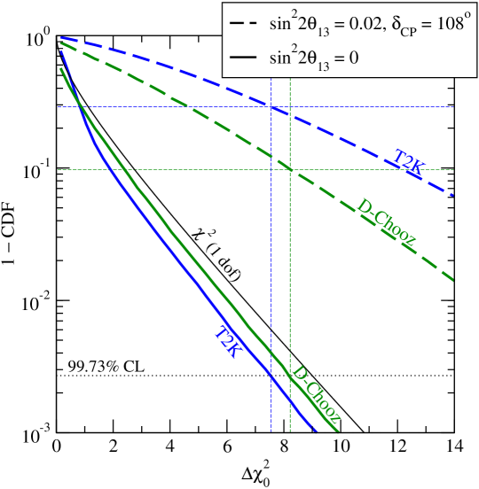
If the experiment had been performed already and real data were available one would now check if $\chi^{2}(\theta_{\mathrm{13}}=0)-\chi^{2}_{\mathrm{min,data}}$ is larger than $\lambda(\alpha)$ to decide whether the hypothesis $\theta_{13}=0$ can be excluded. In the absence of real data one can, however, calculate the probability for this to occur as a function of the value of $\theta_{13}$. More precisely, assuming a fixed value of $\theta_{13}$ (and in case of T2K also of $\delta_{\mathrm{CP}}$) many artificial data sets are generated. This yields the distribution $f_{\theta_{13}}(\Delta\chi^{2}_{0})$ under the assumption of the “true value” $\theta_{13}$. The probability $P_{\mathrm{disc}}(\alpha,\theta_{13})$ that $\theta_{13}=0$ can be excluded at the $100(1-\alpha)\%$ CL is given by

$$P_{\mathrm{disc}}(\alpha,\theta_{13})\equiv P\left[\Delta\chi^{2}_{0}>\lambda(\alpha)\>|\>\theta_{13}\right]=\int_{\lambda(\alpha)}^{\infty}dx\,f_{\theta_{13}}(x)\,.$$ (3)

The calculation of $P_{\mathrm{disc}}$ is illustrated in Fig. 1 assuming that the true value of $\sin^{2}2\theta_{13}$ is 0.02. One can read off from this figure that the probability to exclude the hypothesis $\theta_{13}=0$ at 99.73% CL is about 29% for T2K (if $\delta_{\mathrm{CP}}=108^{\circ}$) and 9.7% for D-Chooz.

Now one has to scan over the true values of $\theta_{13}$ (and in the case of T2K also over $\delta_{\mathrm{CP}}$), repeating the procedure outlined above in each point. Fig. 2 shows the probability $P_{\mathrm{disc}}$ to exclude the hypothesis $\theta_{13}=0$ at the 99.73% CL for T2K and D-Chooz as a function of the true value of $\sin^{2}2\theta_{13}$. For each true value $3\times 10^{6}$ data sets have been simulated. For T2K the two values chosen for $\delta_{\mathrm{CP}}$ correspond roughly to the best and worst sensitivity. The vertical lines in the plot show the standard sensitivities calculated from the condition $\Delta\chi^{2}\geq 9$ without statistical fluctuations. One observes that for D-Chooz the standard sensitivity corresponds indeed with good accuracy to $P_{\mathrm{disc}}=50\%$, as expected for an “average” experiment. For T2K the discovery probabilities corresponding to the standard sensitivities are actually slightly higher, around 60%.

Figure 2: The probability to exclude the hypothesis $\theta_{13}=0$ at the 99.73% CL for T2K and D-Chooz as a function of the true value of $\sin^{2}2\theta_{13}$. The two curves for T2K correspond to the true values $\delta_{\mathrm{CP}}=108^{\circ}$ and $288^{\circ}$. The vertical lines show the corresponding “standard” sensitivities. The dashed curves correspond to the probability $P_{\mathrm{disc}}$ calculated in the Gaussian approximation according to Eq. (4).

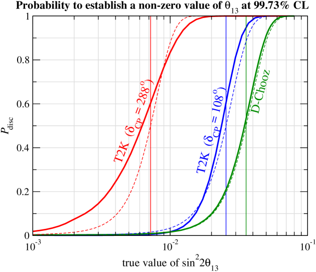
The dashed curves shown in Fig. 2 are obtained assuming a Gaussian measurement of $\sin^{2}2\theta_{13}$. In this case $P_{\mathrm{disc}}$ can be obtained in terms of the error function in the following way. Assuming that $x$ is a Gaussian variable with standard deviation $\sigma$ the hypothesis $x=0$ can be excluded at the 99.73% CL if the observed value $x^{\mathrm{obs}}$ is bigger than $3\sigma$. On the other hand, the probability for $x^{\mathrm{obs}}\geq 3\sigma$ as a function of the true value $x^{\mathrm{true}}$ is easily calculated as

$$P\left[x^{\mathrm{obs}}\geq 3\sigma\>|\>x^{\mathrm{true}}\right]=\int_{3\sigma}^{\infty}dx\,G(x;\>x^{\mathrm{true}},\sigma)=\frac{1}{2}\left[1-\mathrm{erf}\left(\frac{3\sigma-x^{\mathrm{true}}}{\sqrt{2}\sigma}\right)\right]\,,$$ (4)

where $G(x;\>x^{\mathrm{true}},\sigma)$ denotes the normal distribution with mean $x^{\mathrm{true}}$ and standard deviation $\sigma$.

The dashed curves in Fig. 2 have been obtained from Eq. (4) by identifying $\sin^{2}2\theta_{13}=x$ and by using for $\sigma$ one third of the 99.73% CL sensitivity limit from the standard procedure. One observes that for D-Chooz this approximation is excellent. Hence, in this case $\sin^{2}2\theta_{13}$ can be considered indeed as a Gaussian variable and the probability $P_{\mathrm{disc}}$ can be calculated from the standard sensitivity limit and Eq. (4) without the need of a MC simulation. In contrast, for T2K some deviations from Gaussianity are visible (especially for $\delta_{\mathrm{CP}}^{\mathrm{true}}=288^{\circ}$). This is not unexpected, since in this case event numbers are small, background fluctuations are important, and the dependence of the observables on the parameters is much more complicated than in the case of D-Chooz.

Figure 3: Contours of the probability $P_{\mathrm{disc}}$ to establish a non-zero value of $\theta_{31}$ at the 99.73% CL for T2K in the $\sin^{2}2\theta_{13}^{\mathrm{true}}$-$\delta_{\mathrm{CP}}^{\mathrm{true}}$ plane. The dashed curve corresponds to the “standard sensitivity limit”.

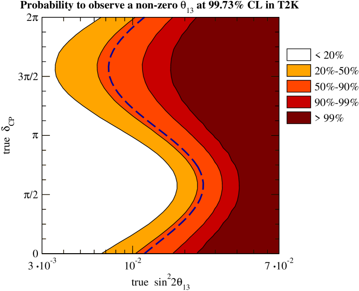
Contours of the probability $P_{\mathrm{disc}}$ for the T2K experiment in the plane of $\sin^{2}2\theta_{13}^{\mathrm{true}}$ and $\delta_{\mathrm{CP}}^{\mathrm{true}}$ are shown in Fig. 3. $P_{\mathrm{disc}}$ has been calculated for a grid of $41\times 41$ values and at each point in the grid $10^{5}$ data sets have been generated, leading in total to nearly $1.7\times 10^{8}$ performed fits. This figure is the generalisation of the usual sensitivity limit (shown as dashed curve) and for each true value of the parameters one can infer the probability that T2K can establish a non-zero value of $\theta_{13}$ at the 99.73% CL. As indicated already in Fig. 2 one finds that the standard sensitivity curve corresponds roughly to a discovery probability of 60%. The region where $\theta_{13}>0$ can be established with high probability, let’s say greater than 99%, is found for $\sin^{2}2\theta_{13}^{\mathrm{true}}>0.0166-0.041$, depending on the true value of $\delta_{\mathrm{CP}}$. It is shifted with respect to the standard sensitivity limit to values of $\sin^{2}2\theta_{13}$ larger by roughly a factor of 2.

4 Sensitivity to CP violation

In this section I will apply similar concepts to the sensitivity to CP violation (CPV), using as example the T2HK experiment. Now the relevant question is:

Given true values of $\theta_{13}$ and $\delta_{\mathrm{CP}}$, what is the probability that CPV can be established at a certain confidence level?

In this case the hypothesis to be excluded, CP conservation (CPC), is more complicated than in the case of the $\theta_{13}$ sensitivity. Whereas in the previous case the hypothesis was just a single point in the parameter space ($\theta_{13}=0$, independent of $\delta_{\mathrm{CP}}$), now one wants to exclude $\delta_{\mathrm{CP}}=0$ and $\delta_{\mathrm{CP}}=\pi$ for any value of $\theta_{13}$. Therefore, in the following the phrase “establish CPV at the $100(1-\alpha)\%$ CL” is considered to be equivalent to the statement that for any value of $\sin^{2}2\theta_{13}$ neither $\delta_{\mathrm{CP}}=0$ nor $\delta_{\mathrm{CP}}=\pi$ is contained in the confidence regions in the $\sin^{2}2\theta_{13}$-$\delta_{\mathrm{CP}}$ plane at the $100(1-\alpha)\%$ CL. For the construction of the confidence regions the Feldman–Cousins method [7] will be used .

This method is implemented as follows. To decide whether given data are consistent with CPC at the $100(1-\alpha)\%$ CL it is checked if the statistic

$$\Delta\chi^{2}_{\mathrm{CPC}}(\theta_{13},\delta_{\mathrm{CPC}})\equiv\chi^{2}(\theta_{13},\delta_{\mathrm{CPC}})-\chi^{2}_{\mathrm{min}}\quad\text{with}\quad\delta_{\mathrm{CPC}}=0,\pi$$ (5)

fulfils the condition

$$\Delta\chi^{2}_{\mathrm{CPC}}(\theta_{13},\delta_{\mathrm{CPC}})>\lambda(\alpha;\,\theta_{13},\delta_{\mathrm{CPC}})$$ (6)

for all values of $\theta_{13}$, where $\lambda(\alpha;\,\theta_{13},\delta_{\mathrm{CPC}})$ is calculated by MC simulation. Many artificial data sets are generated for the parameters $\delta_{\mathrm{CP}}=0,\pi$ and $\theta_{13}$, to map out the distribution $f_{\mathrm{CPC}}(\Delta\chi^{2}_{\mathrm{CPC}}\>|\>\theta_{13},\delta_{\mathrm{CPC}})$. Then $\lambda(\alpha;\,\theta_{13},\delta_{\mathrm{CPC}})$ is determined by

$$\alpha=\int_{\lambda(\alpha;\,\theta_{13},\delta_{\mathrm{CPC}})}^{\infty}dx\,f_{\mathrm{CPC}}(x\>|\>\theta_{13},\delta_{\mathrm{CPC}})\,.$$ (7)

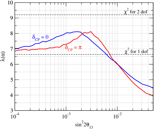
In Fig. 4 $\lambda(\alpha;\,\theta_{13},\delta_{\mathrm{CPC}})$ is shown for $\alpha=0.01$. In contrast to the values 6.635 (9.21) following from $\chi^{2}$-distributions for 1 (2) degrees of freedom the actual cut values vary between 4 and 8.1 in the considered range of $\sin^{2}2\theta_{13}$.

Figure 4: The cut value $\lambda(\alpha;\,\theta_{13},\delta_{\mathrm{CPC}})$, see Eqs. (6) and (7), for the 99% CL ($\alpha=0.01$) as a function of $\sin^{2}2\theta_{13}$ for $\delta_{\mathrm{CP}}=0$ and $\pi$. The horizontal lines show the canonical cut values following from $\chi^{2}$-distributions for 1 and 2 degrees of freedom.

To determine the probability $P_{\mathrm{disc}}$ that CPV can be established for given true values of $\theta_{13}$ and $\delta_{\mathrm{CP}}$ many artificial data sets are generated under the assumption of these parameters. For each data set the test (6) is performed and $P_{\mathrm{disc}}$ is given by the fraction of data sets for which CPV can be established at the corresponding CL. The results of such an analysis for the T2HK experiment are shown in Fig. 5. $P_{\mathrm{disc}}$ has been calculated for a grid of $41\times 41$ true values and at each point in the grid $5\times 10^{4}$ data sets have been generated. This number is somewhat reduced with respect to the one used for the $\theta_{13}$ sensitivity to keep the analysis feasible. Because of the smaller ensemble the CL is reduced to 99%. The plot is restricted to the interval $0\leq\delta_{\mathrm{CP}}\leq\pi$, similar behaviour is expected for $\pi<\delta_{\mathrm{CP}}<2\pi$.

Figure 5: Contours of the probability $P_{\mathrm{disc}}$ to establish CPV at the 99% CL for T2HK in the $\sin^{2}2\theta_{13}^{\mathrm{true}}$-$\delta_{\mathrm{CP}}^{\mathrm{true}}$ plane. The dashed curve corresponds to the “standard sensitivity limit”.

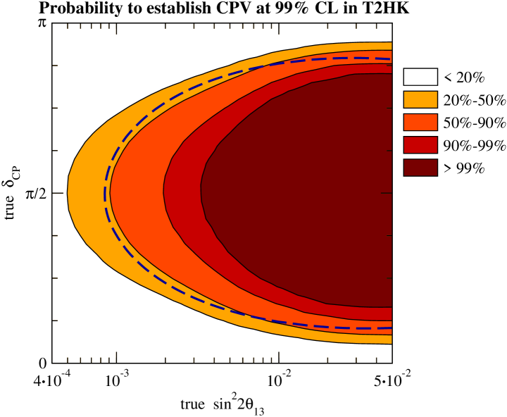
Fig. 5 provides the complete information on the possibilities to discover CPV in T2HK. For each true value of the parameters one can infer the probability that CPV can be establish at the 99% CL. The standard sensitivity limit (obtained from the condition $\Delta\chi^{2}\geq 6.635$ without taking into account statistical fluctuations) is shown as dashed curve. It is remarkable that the standard limit is rather close to the contour for $P_{\mathrm{disc}}=50\%$, i.e., an “average” experiment. The deviations from this value can be motivated from Fig. 4. Since $\lambda(\alpha;\,\theta_{13},\delta_{\mathrm{CPC}})$ is bigger than the canonical value 6.635 for $\sin^{2}2\theta_{13}\lesssim 10^{-2}$ the sensitivity to CPV is actually slightly worse leading to $P_{\mathrm{disc}}<50\%$ for the standard limit, whereas for $\sin^{2}2\theta_{13}\gtrsim 10^{-2}$ one has $\lambda(\alpha;\,\theta_{13},\delta_{\mathrm{CPC}})<6.635$ which leads to better sensitivities to CPV and hence $P_{\mathrm{disc}}>50\%$ at the standard limit.

Despite the rather good approximation of the standard sensitivity limit for $P_{\mathrm{disc}}=50\%$ it is evident from Fig. 5 that one has to be aware of the correct interpretation of such limits. The region where CPV can be established with high probability is significantly smaller than the standard sensitivity region. For example, maximal CPV $\delta_{\mathrm{CP}}=\pi/2$ can be established with a probability of more than 99% at the 99% CL for $\sin^{2}2\theta_{13}>3.3\times 10^{-3}$, whereas the corresponding standard sensitivity limit is $\sin^{2}2\theta_{13}=8.5\times 10^{-4}$, nearly a factor 4 smaller.

5 Summary

In this work the sensitivity of future neutrino oscillation experiments has been calculated by using a statistical procedure within a frequentist framework based on MC simulations. I have determined the probability that a discovery will be made at a given CL as a function of the true parameter values by generating a large ensemble of artificial experiments. The interpretation of the widely used “standard” sensitivity limits, where statistical fluctuations are neglected, has been clarified.

As examples I have considered the discovery of a non-zero value for $\theta_{13}$ at the T2K and Double-Chooz experiments. It has been found that for Double-Chooz the Gaussian approximation is very well justified. The usually calculated sensitivity corresponds to the performance of an average experiment (the discovery will be made with a probability of 50%), and the actual discovery probability can be estimated by a simple formula in terms of the error function. In the case of T2K some deviations from Gaussianity are found and the standard sensitivity limits correspond to a discovery probability of about 60%. Similar concepts have been applied to the discovery of CP violation in neutrino oscillations at the T2HK experiment. A definition of “establishing CP violation” based confidence regions according to the Feldman–Cousins prescription has been used.

For all considered cases I have found that standard sensitivity limits provide a reasonable approximation for an average experiment, corresponding to a discovery probability of order 50%. However, one has to be aware of the correct interpretation of such limits. In general the region where a discovery can be made with high probability is significantly smaller than the one corresponding to the standard sensitivity limits.

Acknowledgement

This work has been triggered partially by the talk Ref. [8] and I thank J. Conrad for stimulating communication on the topic of sensitivity limits.