Flavor $S_{4}\otimes Z_{2}$ symmetry and neutrino mixing

Abstract

We present a model of the lepton masses and flavor mixing based on the discrete group $S_{4}\otimes Z_{2}$. In this model, all the charged leptons and neutrinos are assigned to the ${\bf\underline{3}}_{\alpha}$ representation of $S_{4}$ in the Yamanouchi bases. The charged lepton and neutrino masses are mainly determined by the vacuum expectation value structures of the Higgs fields. A nearly tri-bimaximal lepton flavor mixing pattern, which is in agreement with the current experimental results, can be accommodated in our model. The neutrino mass spectrum takes the nearly degenerate pattern, and thus can be well tested in the future precise experiments.

I introduction

To understand the origin of fermion masses and flavor mixing is crucial and essential in modern particle physics. From the analyses[1] of recent neutrino oscillation experiments[2, 3, 4, 5, 6], we have confirmed the large solar mixing angle $\theta_{12}\simeq 34^{\circ}$[7], maximal atmospheric mixing angle $\theta_{23}\simeq 45^{\circ}$ and a very tiny $\theta_{13}$, $\theta_{13}<10^{\circ}$. A very small solar mass squared difference $\Delta m^{2}_{21}\equiv m^{2}_{2}-m^{2}_{1}\simeq 8.0\times 10^{-5}~{}{\rm eV}^{2}$ and an atmospheric mass squared difference $\Delta m^{2}_{32}\equiv m^{2}_{3}-m^{2}_{2}\simeq\pm 2.5\times 10^{-3}~{}{\rm eV}^{2}$ are given by the experimental data[1]. Here the plus and minus signs in front of $\Delta m^{2}_{32}$ correspond to the normal mass hierarchy ($m_{1}<m_{2}<m_{3}$) and inverted mass hierarchy ($m_{3}<m_{1}<m_{2}$) case. Since the standard model predicts massless neutrinos, it is clear that we should extend the standard model to accommodate non-vanishing neutrino masses. Among all possible mechanisms, the seesaw mechanism[8] is a very interesting and elegant one to explain the light neutrino masses. In the framework of the seesaw mechanism, the light left-handed neutrino masses can well be understood by introducing heavy right-handed Majorana neutrinos, and the light neutrino mass matrix is given by

$$M_{\nu}=M_{D}M^{-1}_{R}M^{T}_{D}\ ,$$ (1)

where $M_{D}$ and $M_{R}$ are the Dirac and Majorana mass matrices respectively. The typical mass scales of $M_{R}$ are $10^{14}\sim 10^{16}{\rm GeV}$.

Since the Yukawa structures are not well constrained up to now, to identify the structure of the neutrino mass matrix is one of the main objects in neutrino physics. An interesting and natural way to study the Yukawa coupling and find the underlying physics is the flavor symmetry. Among all possible flavor symmetries, discrete non-Abelian groups such as $S_{3}$[9], $A_{4}$[10] and so on have attracted a lot of attention. Note that most of these models rely on the basis of their group representation, and contain more theoretical parameters than the observables.

The permutation group $S_{4}$, which is formed by the $4!$ permutations, totally contains 24 group elements which belong to five conjugate classes. Therefore it has five irreducible representations (reps). Among these irreducible reps, there are two one-dimensional (${\bf\underline{1}}_{S}$ and ${\bf\underline{1}}_{A}$), one two-dimensional (${\bf\underline{2}}$) and two three-dimensional (${\bf\underline{3}}_{\alpha}$ and ${\bf\underline{3}}_{\beta}$) reps. Here the ‘S’ and ‘A’ mean symmetric and antisymmetric reps respectively. The character table of $S_{4}$ is given in Table 1. In respect that the particles in our model are all assigned to the ${\bf\underline{1}}_{S}$, ${\bf\underline{2}}$ and ${\bf\underline{3}}_{\alpha}$, we list the relevant representation matrices in Appendix A.

The $S_{4}$ models for fermion masses have been discussed by several authors in Refs.[11, 12]. In this note, we adopt the $S_{4}\otimes Z_{2}$ flavor symmetry and assign all the charged leptons, neutrinos and Higgs into the irreducible Yamanouchi bases[13]. Such a compact scheme contains only a few parameters, and therefore it can be examined quite well in the future experiments.

In the following, we will present the main contents of our model in section II. Some detailed analytical and numerical analyses will be given in section III. In section IV, the $S_{4}$ invariant Higgs potential are discussed. Finally, a brief summary is given in section V.

II particle assignment

In our model, all the leptons are assigned to the $\underline{\bf 3}_{\alpha}$ rep of $S_{4}$, but their $Z_{2}$ charges are different. Under the group

$$G=SU(3)_{c}\otimes SU(2)_{L}\otimes U(1)_{Y}\otimes S_{4}\otimes Z_{2}\ ,$$ (2)

the lepton contents in our model are placed as

$$\ell_{L} \sim (1,2,-1)(\underline{\bf 3}_{\alpha},+)\ ,$$ (3)

$$e_{R} \sim (1,1,-2)(\underline{\bf 3}_{\alpha},+)\ ,$$ (4)

$$\nu_{R} \sim (1,1,0)(\underline{\bf 3}_{\alpha},-)\ ,$$ (5)

where the plus or minus sign denotes the reflection properties under $Z_{2}$, i.e. $\Psi\rightarrow\pm\Psi$. The Higgs scalars in our model are placed as follows

$$H_{u} \sim (1,2,-1)(\underline{\bf 1}_{\bf S},+)\ ,$$ (6)

$$H_{d} \sim (1,2,-1)(\underline{\bf 1}_{\bf S},-)\ ,$$ (7)

$$\chi \sim (1,2,-1)(\underline{\bf 3}_{\alpha},-)\ ,$$ (8)

$$\phi \sim (1,2,-1)(\underline{\bf 2},+)\ .$$ (9)

Here the $Z_{2}$ symmetry guarantees that the lepton doublet couples to ($e_{R},\phi_{i}$) and ($\nu_{R},\chi_{i}$) respectively. It will be shown in section IV that the masses of Higgs scalars are almost unconstrained in this model, thus we can choose their masses at some high energy scales in order to avoid the tree level flavor charging neutral currents. Note that we do not introduce any $SU(2)_{L}$ singlet or triplet Higgs[14]. Hence the Heavy right-handed neutrino masses are exactly degenerate.

By using the group algebra given in Appendix A, we write down the $S_{4}\otimes Z_{2}$ invariant Yukawa couplings:

$$-{\cal L}_{Y}=\alpha_{e}\overline{\ell_{iL}}e_{iR}\tilde{H_{u}}+\beta_{e}f_{ijk}\overline{\ell_{iL}}e_{jR}\tilde{\phi_{k}}+\alpha_{\nu}\overline{\ell_{iL}}\nu_{iR}{H_{d}}+\beta_{\nu}g_{ijk}\overline{\ell_{iL}}\nu_{jR}{\chi_{k}}+\frac{1}{2}M\overline{\nu^{c}_{iR}}\nu_{iR}+h.c.$$ (10)

where $\tilde{H}_{u}=i\tau_{2}H^{*}_{u}$ and $\tilde{\phi}=i\tau_{2}\phi^{*}$. The last term in Eq. (5) is the bare Majorana mass term with $M$ being the typical mass scale of the heavy right-handed neutrinos. The coefficients $\alpha_{e,\nu}$ and $\beta_{e,\nu}$ are in general complex parameters. However, since their phases are all global phases, there will be no Dirac CP violating phases in the MNS matrix and only the Majorana phases can be accommodated up to now. The structures of the traceless matrices $f$ and $g$ can be obtained from the CG coefficients of $S_{4}$. Following the CG coefficient tables given in Ref. [13], we arrive at

$$f_{ij1}=\left(\matrix{0&\sqrt{2}&0\cr\sqrt{2}&1&0\cr 0&0&-1}\right)\ ,\ \ \ \ \ f_{ij2}=\left(\matrix{0&0&\sqrt{2}\cr 0&0&-1\cr\sqrt{2}&-1&0}\right)\ ,$$ (11)

and

$$g_{ij1} = \left(\matrix{2&0&0\cr 0&-1&0\cr 0&0&-1}\right)\ ,\ \ \ \ \ g_{ij2}=\left(\matrix{0&-1&0\cr-1&\sqrt{2}&0\cr 0&0&-\sqrt{2}}\right)\ ,$$ (12)

$$g_{ij3} = \left(\matrix{0&0&-1\cr 0&0&-\sqrt{2}\cr-1&-\sqrt{2}&0}\right)\ ,$$ (13)

where all the coefficient matrices are symmetric and traceless. Hence both the charged lepton and neutrino mass matrices are symmetric.

As we have mentioned above, the right-handed neutrino masses are exactly degenerate by now. Such a result is not favored in some leptogenesis models[16] in which the mass splits of the heavy right-handed neutrinos are required. This drawback can easily be solved by introducing an additional Higgs scalar $\eta\sim(1,1,0)(\underline{\bf 2},+)$ or $\xi\sim(1,1,0)(\underline{\bf 3}_{\alpha},+)$ which couples to $\nu_{R}$ in the form of

$$-{\cal L}_{\eta-\nu_{R}}=\beta_{R}f_{ijk}\overline{\nu^{c}_{iR}}\nu_{jR}\eta_{k}\ ,$$ (14)

or

$$-{\cal L}_{\xi-\nu_{R}}=\beta_{R}g_{ijk}\overline{\nu^{c}_{iR}}\nu_{jR}\xi_{k}\ .$$ (15)

Their vacuum expectation values(VEVs) will bring the mass splits of right-handed neutrinos and the phases of $\beta_{R}$ will lead to the Dirac CP violating phases in the MNS matrix.

Another possible way to gain the mass differences of the right-handed neutrinos is to consider the renormalization group equation running effects[17] which can usually be used to generate a small mass split in the resonant leptogenesis models[18]. A Dirac CP violating phase can also be gained at the same time from the renormalization group equation running[19].

In our analyses, we focus our attention on the low energy phenomena of our model. So we assume that all the Yukawa couplings are real and the right-handed neutrino masses are exactly degenerate.

III lepton mass matrices and mixing matrix

Assuming the flavor symmetry $S_{4}$ is broken by the VEVs of the Higgs scalars in the form of $\left<H_{u}\right>=v_{u}$, $\left<H_{d}\right>=v_{d}$, $\left<\phi_{i}\right>=u_{i}$ and $\left<\chi_{i}\right>=w_{i}$, we obtain the mass matrix of the charged leptons as

$$M_{l}=\left(\matrix{a&\sqrt{2}x_{1}&\sqrt{2}x_{2}\cr\sqrt{2}x_{1}&a+x_{1}&-x_{2}\cr\sqrt{2}x_{2}&-x_{2}&a-x_{1}}\right)\ ,$$ (16)

where $a$ and $x_{i}$ are defined by $a=\alpha_{e}v_{u}$ and $x_{i}=\beta_{e}u_{i}$ respectively.

The Dirac mass matrix of the neutrinos is given by

$$M_{D}=\left(\matrix{2y_{1}+b&-y_{2}&-y_{3}\cr-y_{2}&\sqrt{2}y_{2}-y_{1}+b&-\sqrt{2}y_{3}\cr-y_{3}&-\sqrt{2}y_{3}&-y_{1}-\sqrt{2}y_{2}+b}\right)\ ,$$ (17)

where $b=\alpha_{\nu}v_{d}$ and $y_{i}=\beta_{\nu}w_{i}$. Taking account of the seesaw relation in Eq. (1), we obtain the light neutrino mass matrix:

$$M_{\nu}=m_{0}\left(\matrix{(2+\epsilon)^{2}+r^{2}+s^{2}&\sqrt{2}s^{2}-(1+2\epsilon+\sqrt{2}r)r&-(1+2\epsilon-2\sqrt{2}r)s\cr\sim&(1-\epsilon-\sqrt{2}r)^{2}+r^{2}+2s^{2}&(2\sqrt{2}-2\sqrt{2}\epsilon+r)s\cr\sim&\sim&(1-\epsilon+\sqrt{2}r)^{2}+3s^{2}}\right)\ ,$$ (18)

where $m_{0}=y^{2}_{1}/M$, $\epsilon=b/y_{1}$, $r=y_{2}/y_{1}$ and $s=y_{3}/y_{1}$. Note that all the lepton mass matrices are symmetric.

The mass matrices $M_{l}$ and $M_{\nu}$ can respectively be diagonalized by two unitary matrices $V_{l}$ and $V_{\nu}$: $V^{\dagger}_{l}M_{l}V^{\ast}_{l}={\rm Diag}\{m_{e},m_{\mu},m_{\tau}\}$, $V^{\dagger}_{\nu}M_{\nu}V^{\ast}_{\nu}={\rm Diag}\{m_{1},m_{2},m_{3}\}$. The lepton flavor mixing matrix $V_{\rm MNS}$, which links the neutrino mass eigenstates ($\nu_{1},\nu_{2},\nu_{3}$) with their flavor eigenstates ($\nu_{e},\nu_{\mu},\nu_{\tau}$), is then given by $V_{\rm MNS}=V^{{\dagger}}_{l}V_{\nu}$.

A charged lepton sector

By diagonalizing the charged lepton mass matrix in Eq. (10), we get the charged lepton masses:

$$m_{e} = a+2x_{1}\ ,$$ (19)

$$m_{\mu} = a-x_{1}+\sqrt{3}x_{2}\ ,$$ (20)

$$m_{\tau} = a-x_{1}-\sqrt{3}x_{2}\ ,$$ (21)

and the mixing matrix $V_{l}$:

$$V_{l}=\left(\matrix{\displaystyle\frac{1}{\sqrt{3}}&\displaystyle\frac{1}{\sqrt{3}}&\displaystyle\frac{1}{\sqrt{3}}\cr\displaystyle\frac{2}{\sqrt{6}}&\displaystyle-\frac{1}{\sqrt{6}}&\displaystyle-\frac{1}{\sqrt{6}}\cr 0&\displaystyle\frac{1}{\sqrt{2}}&\displaystyle-\frac{1}{\sqrt{2}}}\right)\ .$$ (22)

A typical interesting and instructive feature is that $V_{l}$ is a constant matrix with respective to arbitrary $a$ and $x_{i}$. After being transposed, this matrix takes the very similar form to the tri-bimaximal mixing matrix[20]

$$V_{\rm tri-bi}=\left(\matrix{\displaystyle\frac{2}{\sqrt{6}}&\displaystyle\frac{1}{\sqrt{3}}&0\cr\cr\displaystyle-\frac{1}{\sqrt{6}}&\displaystyle\frac{1}{\sqrt{3}}&\displaystyle\frac{1}{\sqrt{2}}\cr\cr\displaystyle-\frac{1}{\sqrt{6}}&\displaystyle\frac{1}{\sqrt{3}}&\displaystyle-\frac{1}{\sqrt{2}}\cr}\right)\;,$$ (23)

only up to an exchange between the first and second column.

By using Eq. (13), we can also express the parameters $a$, $x_{1}$ and $x_{2}$ in terms of the charged lepton masses as

$$a = \frac{1}{3}\left(m_{e}+m_{\mu}+m_{\tau}\right)\ ,$$ (24)

$$x_{1} = \frac{1}{6}\left(2m_{e}-m_{\mu}-m_{\tau}\right)\ ,$$ (25)

$$x_{2} = \frac{1}{2\sqrt{3}}\left(m_{\mu}-m_{\tau}\right)\ .$$ (26)

Considering the mass hierarchies of the charged leptons: $m_{\tau}\gg m_{\mu}\gg m_{e}$, it is easy to conclude that $|a|>|x_{2}|>|x_{1}|$.

B neutrino sector

As an example, we assume $s=0$ and $r\ll 1$ . Then, $M_{D}$ takes the simple form:

$$M_{D}=y_{1}\left(\matrix{2+\epsilon&-r&0\cr-r&-1+\sqrt{2}r+\epsilon&0\cr 0&0&-1-\sqrt{2}r+\epsilon}\right)\ ,$$ (27)

and the light neutrino mass matrix can be written as

$$M_{\nu}=m_{0}\left(\matrix{(2+\epsilon)^{2}+r^{2}&-r-2r\epsilon-\sqrt{2}r^{2}&0\cr-r-2r\epsilon-\sqrt{2}r^{2}&(1-\epsilon-\sqrt{2}r)^{2}+r^{2}&0\cr 0&0&(1-\epsilon+\sqrt{2}r)^{2}}\right)\ .$$ (28)

There are two texture zeros in the third row of $M_{\nu}$[21]. Therefore only the mixing between the first two generations exists in the neutrino sector. After straightforward calculations, we obtain the light neutrino masses:

$$m_{1} \simeq m_{0}\left[(1-\epsilon)^{2}-2\sqrt{2}(1-\epsilon)r+\frac{2}{3}(4-\epsilon)r^{2}\right]\ ,$$ (29)

$$m_{2} \simeq m_{0}\left[(2+\epsilon)^{2}+\frac{2}{3}(2+\epsilon)r^{2}\right]\ ,$$ (30)

$$m_{3} \simeq m_{0}\left[(1-\epsilon)^{2}+2\sqrt{2}(1-\epsilon)r+2r^{2}\right]\ ,$$ (31)

where the terms in proportion to $r^{3}$ have been neglected. The mixing matrix $V_{\nu}$ can be approximated to

$$V_{\nu}\simeq\left(\matrix{\displaystyle\frac{1}{3}r+\frac{\sqrt{2}}{9}r^{2}&\displaystyle-1+\frac{1}{18}r^{2}&0\cr\displaystyle 1-\frac{1}{18}r^{2}&\displaystyle\frac{1}{3}r+\frac{\sqrt{2}}{9}r^{2}&\displaystyle 0\cr 0&0&1}\right)+{\cal O}(r^{3})\ .$$ (32)

It is interesting that only the parameter $r$ appears in the approximate expression of $V_{\nu}$.

The MNS mixing matrix is given by

$$V_{\rm MNS} = V^{\dagger}_{l}V_{\nu}=\left[V^{\dagger}_{l}.\left(\matrix{0&1&0\cr 1&0&0\cr 0&0&1}\right)\right]\cdot\left[\left(\matrix{0&1&0\cr 1&0&0\cr 0&0&1}\right)V_{\nu}\right]$$ (33)

$$= \left(\matrix{\displaystyle\frac{2}{\sqrt{6}}&\displaystyle\frac{1}{\sqrt{3}}&0\cr\cr\displaystyle-\frac{1}{\sqrt{6}}&\displaystyle\frac{1}{\sqrt{3}}&\displaystyle\frac{1}{\sqrt{2}}\cr\cr\displaystyle-\frac{1}{\sqrt{6}}&\displaystyle\frac{1}{\sqrt{3}}&\displaystyle-\frac{1}{\sqrt{2}}\cr}\right)\cdot\left(\matrix{\displaystyle 1-\frac{1}{18}r^{2}&\displaystyle\frac{1}{3}r+\frac{\sqrt{2}}{9}r^{2}&\displaystyle 0\cr\displaystyle\frac{1}{3}r+\frac{\sqrt{2}}{9}r^{2}&\displaystyle-1+\frac{1}{18}r^{2}&0\cr 0&0&1}\right)$$ (34)

$$= V_{\rm tri-bi}\cdot\left(\matrix{\cos\theta&\sin\theta&0\cr-\sin\theta&\cos\theta&0\cr 0&0&1}\right)\cdot\left(\matrix{1&0&0\cr 0&-1&0\cr 0&0&1}\right)\ ,$$ (35)

where

$$\sin\theta = -\frac{1}{3}r-\frac{\sqrt{2}}{9}r^{2}\ ,$$ (36)

$$\cos\theta = 1-\frac{1}{18}r^{2}\ .$$ (37)

The last matrix in Eq. (21) contributes a trivial phase $\pm\pi$ in the MNS matrix, thus it can be safely neglected without changing any phisics. The explicit expression of $V_{\rm MNS}$ is

$$V_{\rm MNS}=\left(\matrix{\displaystyle\frac{2\cos\theta}{\sqrt{6}}-\frac{\sin\theta}{\sqrt{3}}&\displaystyle\frac{\cos\theta}{\sqrt{3}}+\frac{2\sin\theta}{\sqrt{6}}&0\cr\displaystyle\frac{-\cos\theta}{\sqrt{6}}-\frac{\sin\theta}{\sqrt{3}}&\displaystyle\frac{\cos\theta}{\sqrt{3}}-\frac{\sin\theta}{\sqrt{6}}&\displaystyle\frac{1}{\sqrt{2}}\cr\displaystyle-\frac{\cos\theta}{\sqrt{6}}-\frac{\sin\theta}{\sqrt{3}}&\displaystyle\frac{\cos\theta}{\sqrt{3}}-\frac{\sin\theta}{\sqrt{6}}&\displaystyle-\frac{1}{\sqrt{2}}}\right)\ .$$ (38)

Comparing Eq. (24) with the standard parametrization

$$V^{\rm sp}_{\rm MNS}=\left(\matrix{c_{12}c_{13}&s_{12}c_{13}&s_{13}e^{-i\delta}\cr-s_{12}c_{23}-c_{12}s_{23}s_{13}e^{i\delta}&c_{12}c_{23}-s_{12}s_{23}s_{13}e^{i\delta}&s_{23}c_{13}\cr s_{12}c_{23}-c_{12}c_{23}s_{13}e^{i\delta}&-c_{12}s_{23}-s_{12}c_{23}s_{13}e^{i\delta}&c_{23}c_{13}}\right)\cdot\left(\matrix{e^{i\rho}&0&0\cr 0&e^{i\sigma}&0\cr 0&0&1}\right)\ ,$$ (39)

we obtain three mixing angles

$$\sin\theta_{12} = \frac{\cos\theta}{\sqrt{3}}+\frac{2\sin\theta}{\sqrt{6}}\ ,$$ (40)

$$\sin\theta_{23} = \frac{1}{\sqrt{2}}\ ,$$ (41)

$$\sin\theta_{13} = 0\ ,$$ (42)

together with $\delta=\rho=\sigma=0$.

From the experimental data of $\theta_{12}$ and Eq. (26), we can estimate that $\theta\simeq-1.4^{\circ}$. These results depend on ours assumptions. It should be emphasized that $\theta_{13}$ will not vanish if we loose our assumptions by setting $s\neq 0$. In this case, small corrections on $\theta_{23}$ will also be given corresponding to the nonzero $s$, and we will illustrate these corrections in the next subsection.

C numerical analyses

In our numerical analyses, we first take the charged lepton pole masses $M^{\rm pole}_{l}$ given by PDG[22], and then evaluate the charged lepton running masses $m_{l}(\mu)$ from $M^{\rm pole}_{l}$ to the $M_{Z}$ scale by using[23]

$$m_{l}(M_{Z})\;=\;M^{\rm pole}_{l}\left[1-\frac{\alpha(M_{Z})}{\pi}\left(\frac{3}{2}\ln\frac{M_{Z}}{m_{l}(M_{Z})}+1\right)\right]\ .$$ (43)

Then we obtain

$$m_{e}(M_{Z}) = 0.4867~{}{\rm MeV}\ ,$$ (44)

$$m_{\mu}(M_{Z}) = 102.7~{}{\rm MeV}\ ,$$ (45)

$$m_{\tau}(M_{Z}) = 1746.6~{}{\rm MeV}\ .$$ (46)

We can directly calculate the parameters ($a,x_{1},x_{2}$) by using Eqs. (16),

$$a \simeq 616.6~{}{\rm MeV}\ ,\ \ \ \ \ x_{1}\simeq-308.0~{}{\rm MeV}\ ,\ \ \ \ \ x_{2}\simeq-474.5~{}{\rm MeV}\ .$$ (47)

For the neutrino sector, we take the light neutrino mass squared differences $\Delta m^{2}_{21}=8.0\times 10^{-5}~{}{\rm eV}^{2}$ and $\Delta m^{2}_{32}=\pm 2.5\times 10^{-3}~{}{\rm eV}^{2}$, three mixing angles $\theta_{12}=33.9^{\circ}$, $\theta_{23}=45^{\circ}$ and $\theta_{13}=0^{\circ}$[1] as the input values. We firstly consider the case $s=0$. By combining Eqs. (19), (22) and (23), after some numerical calculations, we find that only the normal mass hierarchy case is allowed for our assumptions. The corresponding parameters are

$$m_{0} \simeq 2.99\times 10^{-2}~{}{\rm eV}\ ,\ \ \ \ \ r\simeq 6.92\times 10^{-2}\ ,\ \ \ \ \ \epsilon\simeq-0.545\ .$$ (48)

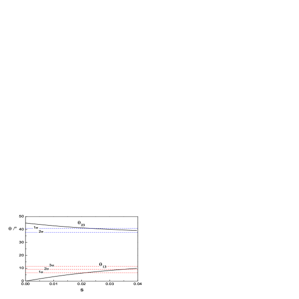
It can be seen clearly that our assumption $r\ll 1$ is quite reasonable. The lightest neutrino mass is $m_{1}\simeq 0.063~{}{\rm eV}$. Hence the neutrinos have a nearly degenerate mass spectrum: $m_{1}\simeq m_{2}\simeq m_{3}$. As for the case $s\neq 0$, the mixing angles $\theta_{13}$ and $\theta_{23}$ will in general get corrections and deviate from their tribi-maximal values. In Fig. 1, we show the corrections on $\theta_{13}$ and $\theta_{23}$ from nonzero $s$. We can find that $\theta_{13}$ is more sensitive to the non-vanishing $s$, and in order to get a nonzero $\theta_{13}$ within 1 and 2$\sigma$ confidence level $s$ should not be larger than 0.02 and 0.035.

Note that the predictions of our model rely on the VEV structures of the Higgs fields. Here we have assumed that such conditions on the VEVs of the Higgs scalars can be well satisfied. In section IV, a detailed analysis will be given to show that this kind of VEV configuration can be obtained by a suitable choice of parameters of the Higgs potential. As mentioned above, in our analyses we do not consider the CP violation of our model. To generalize our model to the CP violating case, we can add the singlet Higgs scalar given by Eq. (8) or (9) and insert the phase factors into the parameters $\alpha$ and $\beta$ in Eq. (5). In this case, the mass splits of the right-handed neutrinos and the CP violation in the neutrino mixing can be acquired simultaneously. As a consequence, there will be more freedom to fit the experimental data and one may test the leptogenesis mechanism within this framework. Such an extension may be more interesting and the corresponding detailed analyses will be elaborated elsewhere.

IV higgs potential

The most general $S_{4}\otimes Z_{2}$ invariant Higgs potential in our model is given by

$$V = -m^{2}_{u}(H^{\dagger}_{u}H_{u})-m^{2}_{d}(H^{\dagger}_{d}H_{d})-m^{2}_{\phi}\sum^{2}_{i=1}\phi^{\dagger}_{i}\phi_{i}-m^{2}_{\chi}\sum^{3}_{j=1}\chi^{\dagger}_{j}\chi_{j}$$ (49)

$$+ \lambda_{u}(H^{\dagger}_{u}H_{u})^{2}+\lambda_{d}(H^{\dagger}_{d}H_{d})^{2}+\lambda_{\phi}\left(\sum^{2}_{i=1}\phi^{\dagger}_{i}\phi_{i}\right)^{2}+\lambda_{\chi}\left(\sum^{3}_{j=1}\chi^{\dagger}_{j}\chi_{j}\right)^{2}$$ (50)

$$+ \tau_{1}\left[(\phi^{\dagger}_{1}\phi_{1}-\phi^{\dagger}_{2}\phi_{2})^{2}+(\phi^{\dagger}_{1}\phi_{2}+\phi^{\dagger}_{2}\phi_{1})^{2}\right]+\tau_{2}(\phi^{\dagger}_{1}\phi_{2}-\phi^{\dagger}_{2}\phi_{1})^{2}$$ (51)

$$+ \mu_{1}\left[(2\chi^{\dagger}_{1}\chi_{1}-\chi^{\dagger}_{2}\chi_{2}-\chi^{\dagger}_{3}\chi_{3})^{2}+(\chi^{\dagger}_{1}\chi_{2}+\chi^{\dagger}_{2}\chi_{1}-\sqrt{2}\chi^{\dagger}_{2}\chi_{2}+\sqrt{2}\chi^{\dagger}_{3}\chi_{3})^{2}\right.$$ (52)

$$+ \left.(\chi^{\dagger}_{1}\chi_{3}+\chi^{\dagger}_{3}\chi_{1}+\sqrt{2}\chi^{\dagger}_{2}\chi_{3}+\sqrt{2}\chi^{\dagger}_{3}\chi_{2})^{2}\right]$$ (53)

$$+ \mu_{2}\left[(\chi^{\dagger}_{1}\chi_{2}-\chi^{\dagger}_{2}\chi_{1})^{2}+(\chi^{\dagger}_{1}\chi_{3}-\chi^{\dagger}_{3}\chi_{1})^{2}+(\chi^{\dagger}_{2}\chi_{3}-\chi^{\dagger}_{3}\chi_{2})^{2}\right]$$ (54)

$$+ \mu_{3}\left[(\chi^{\dagger}_{2}\chi_{2}-\chi^{\dagger}_{3}\chi_{3}+\sqrt{2}\chi^{\dagger}_{1}\chi_{2}+\sqrt{2}\chi^{\dagger}_{2}\chi_{1})^{2}+(\chi^{\dagger}_{2}\chi_{3}+\chi^{\dagger}_{3}\chi_{2}-\sqrt{2}\chi^{\dagger}_{1}\chi_{3}-\sqrt{2}\chi^{\dagger}_{3}\chi_{1})^{2}\right]$$ (55)

$$+ \lambda_{1}(H^{\dagger}_{u}H_{u})(H^{\dagger}_{d}H_{d})+\lambda_{2}(H^{\dagger}_{u}H_{d})(H^{\dagger}_{d}H_{u})+\left[\lambda_{3}(H^{\dagger}_{u}H_{d})^{2}+{\rm h.c.}\right]$$ (56)

$$+ \lambda^{\phi}_{1}(H^{\dagger}_{u}H_{u})\left(\sum^{2}_{i=1}\phi^{\dagger}_{i}\phi_{i}\right)+\left\{\lambda^{\phi}_{2}\left[(H^{\dagger}_{u}\phi_{1})^{2}+(H^{\dagger}_{u}\phi_{2})^{2}\right]+{\rm h.c.}\right\}+\lambda^{\phi}_{3}\left(\left|H^{\dagger}_{u}\phi_{1}\right|^{2}+\left|H^{\dagger}_{u}\phi_{2}\right|^{2}\right)$$ (57)

$$+ \left\{\lambda^{\phi}_{4}\left[(H^{\dagger}_{u}\phi_{1})(\phi^{\dagger}_{1}\phi_{1}-\phi^{\dagger}_{2}\phi_{2})-(H^{\dagger}_{u}\phi_{2})(\phi^{\dagger}_{1}\phi_{2}+\phi^{\dagger}_{2}\phi_{1})\right]+{\rm h.c.}\right\}$$ (58)

$$+ \lambda^{\chi}_{1}(H^{\dagger}_{u}H_{u})\left(\sum^{3}_{i=1}\chi^{\dagger}_{i}\chi_{i}\right)+\left\{\lambda^{\chi}_{2}\left[(H^{\dagger}_{u}\chi_{1})^{2}+(H^{\dagger}_{u}\chi_{2})^{2}+(H^{\dagger}_{u}\chi_{3})^{2}\right]+{\rm h.c.}\right\}$$ (59)

$$+ \lambda^{\chi}_{3}\left(\left|H^{\dagger}_{u}\chi_{1}\right|^{2}+\left|H^{\dagger}_{u}\chi_{2}\right|^{2}+\left|H^{\dagger}_{u}\chi_{3}\right|^{2}\right)$$ (60)

$$+ \sigma^{\phi}_{1}(H^{\dagger}_{d}H_{d})\left(\sum^{2}_{i=1}\phi^{\dagger}_{i}\phi_{i}\right)+\left\{\sigma^{\phi}_{2}\left[(H^{\dagger}_{d}\phi_{1})^{2}+(H^{\dagger}_{d}\phi_{2})^{2}\right]+{\rm h.c.}\right\}+\sigma^{\phi}_{3}\left(\left|H^{\dagger}_{d}\phi_{1}\right|^{2}+\left|H^{\dagger}_{d}\phi_{2}\right|^{2}\right)$$ (61)

$$+ \sigma^{\chi}_{1}(H^{\dagger}_{d}H_{d})\left(\sum^{3}_{i=1}\chi^{\dagger}_{i}\chi_{i}\right)+\left\{\sigma^{\chi}_{2}\left[(H^{\dagger}_{d}\chi_{1})^{2}+(H^{\dagger}_{d}\chi_{2})^{2}+(H^{\dagger}_{d}\chi_{3})^{2}\right]+{\rm h.c.}\right\}$$ (62)

$$+ \sigma^{\chi}_{3}\left(\left|H^{\dagger}_{d}\chi_{1}\right|^{2}+\left|H^{\dagger}_{d}\chi_{2}\right|^{2}+\left|H^{\dagger}_{d}\chi_{3}\right|^{2}\right)$$ (63)

$$+ \left\{\sigma^{\chi}_{4}\left[(H^{\dagger}_{d}\chi_{1})(2\chi^{\dagger}_{1}\chi_{1}-\chi^{\dagger}_{2}\chi_{2}-\chi^{\dagger}_{3}\chi_{3})-(H^{\dagger}_{d}\chi_{2})(\chi^{\dagger}_{1}\chi_{2}+\chi^{\dagger}_{2}\chi_{1}-\sqrt{2}\chi^{\dagger}_{2}\chi_{2}+\sqrt{2}\chi^{\dagger}_{3}\chi_{3})\right.\right.$$ (64)

$$- \left.\left.(H^{\dagger}_{d}\chi_{3})(\chi^{\dagger}_{1}\chi_{3}+\chi^{\dagger}_{3}\chi_{1}+\sqrt{2}\chi^{\dagger}_{2}\chi_{3}+\sqrt{2}\chi^{\dagger}_{3}\chi_{2})\right]+{\rm h.c.}\right\}$$ (65)

$$+ \kappa_{1}\left(\sum^{2}_{i=1}\phi^{\dagger}_{i}\phi_{i}\right)\left(\sum^{3}_{j=1}\chi^{\dagger}_{j}\chi_{j}\right)+\left\{\kappa_{2}\left[(\phi^{\dagger}_{1}\phi_{1}-\phi^{\dagger}_{2}\phi_{2})(\chi^{\dagger}_{2}\chi_{2}-\chi^{\dagger}_{3}\chi_{3}+\sqrt{2}\chi^{\dagger}_{1}\chi_{2}+\sqrt{2}\chi^{\dagger}_{2}\chi_{1})\right.\right.$$ (66)

$$+ \left.\left.(\phi^{\dagger}_{1}\phi_{2}+\phi^{\dagger}_{2}\phi_{1})(\chi^{\dagger}_{2}\chi_{3}+\chi^{\dagger}_{3}\chi_{2}-\sqrt{2}\chi^{\dagger}_{1}\chi_{3}-\sqrt{2}\chi^{\dagger}_{3}\chi_{1})\right]+{\rm h.c.}\right\}$$ (67)

$$+ \left\{\kappa_{3}\left[2(\phi^{\dagger}_{1}\chi_{2}+\phi^{\dagger}_{2}\chi_{3})^{2}+(\phi^{\dagger}_{1}\chi_{2}-\phi^{\dagger}_{2}\chi_{3}+\sqrt{2}\phi^{\dagger}_{1}\chi_{1})^{2}+(\phi^{\dagger}_{2}\chi_{2}+\phi^{\dagger}_{1}\chi_{3}-\sqrt{2}\phi^{\dagger}_{2}\chi_{1})^{2}\right]+{\rm h.c.}\right\}$$ (68)

$$+ \left\{\kappa_{4}\left[(\phi^{\dagger}_{1}\chi_{2}-\phi^{\dagger}_{2}\chi_{3}-\sqrt{2}\phi^{\dagger}_{1}\chi_{1})^{2}+(\phi^{\dagger}_{2}\chi_{2}+\phi^{\dagger}_{1}\chi_{3}+\sqrt{2}\phi^{\dagger}_{2}\chi_{1})^{2}+2(\phi^{\dagger}_{2}\chi_{2}-\phi^{\dagger}_{1}\chi_{3})^{2}\right]+{\rm h.c.}\right\}$$ (69)

$$+ \kappa_{5}\left[2\left|\phi^{\dagger}_{1}\chi_{2}+\phi^{\dagger}_{2}\chi_{3}\right|^{2}+\left|\phi^{\dagger}_{1}\chi_{2}-\phi^{\dagger}_{2}\chi_{3}+\sqrt{2}\phi^{\dagger}_{1}\chi_{1}\right|^{2}+\left|\phi^{\dagger}_{2}\chi_{2}+\phi^{\dagger}_{1}\chi_{3}-\sqrt{2}\phi^{\dagger}_{2}\chi_{1}\right|^{2}\right]$$ (70)

$$+ \kappa_{6}\left[\left|\phi^{\dagger}_{1}\chi_{2}-\phi^{\dagger}_{2}\chi_{3}-\sqrt{2}\phi^{\dagger}_{1}\chi_{1}\right|^{2}+\left|\phi^{\dagger}_{2}\chi_{2}+\phi^{\dagger}_{1}\chi_{3}+\sqrt{2}\phi^{\dagger}_{2}\chi_{1}\right|^{2}+2\left|\phi^{\dagger}_{2}\chi_{2}-\phi^{\dagger}_{1}\chi_{3}\right|^{2}\right]$$ (71)

$$+ \left\{\delta_{1}\left[(H^{\dagger}_{u}\phi_{1})(\chi^{\dagger}_{2}\chi_{2}-\chi^{\dagger}_{3}\chi_{3}+\sqrt{2}\chi^{\dagger}_{1}\chi_{2}+\sqrt{2}\chi^{\dagger}_{2}\chi_{1})\right.\right.$$ (72)

$$- \left.\left.(H^{\dagger}_{u}\phi_{2})(\chi^{\dagger}_{2}\chi_{3}+\chi^{\dagger}_{3}\chi_{2}-\sqrt{2}\chi^{\dagger}_{1}\chi_{3}-\sqrt{2}\chi^{\dagger}_{3}\chi_{1})\right]+{\rm h.c.}\right\}$$ (73)

$$+ \left\{\delta_{2}\left[\sqrt{2}(H^{\dagger}_{u}\chi_{1})(\phi^{\dagger}_{1}\chi_{2}+\phi^{\dagger}_{2}\chi_{3})+(H^{\dagger}_{u}\chi_{2})(\phi^{\dagger}_{1}\chi_{2}-\phi^{\dagger}_{2}\chi_{3}+\sqrt{2}\phi^{\dagger}_{1}\chi_{1})\right.\right.$$ (74)

$$- \left.\left.(H^{\dagger}_{u}\chi_{3})(\phi^{\dagger}_{1}\chi_{3}+\phi^{\dagger}_{2}\chi_{2}-\sqrt{2}\phi^{\dagger}_{2}\chi_{1})\right]+{\rm h.c.}\right\}$$ (75)

$$+ \left\{\delta_{3}\left[\sqrt{2}(H^{\dagger}_{u}\chi_{1})(\chi^{\dagger}_{2}\phi_{1}+\chi^{\dagger}_{3}\phi_{2})+(H^{\dagger}_{u}\chi_{2})(\chi^{\dagger}_{2}\phi_{1}-\chi^{\dagger}_{3}\phi_{2}+\sqrt{2}\chi^{\dagger}_{1}\phi_{1})\right.\right.$$ (76)

$$- \left.\left.(H^{\dagger}_{u}\chi_{3})(\chi^{\dagger}_{3}\phi_{1}+\chi^{\dagger}_{2}\phi_{2}-\sqrt{2}\chi^{\dagger}_{1}\phi_{2})\right]+{\rm h.c.}\right\}\ .$$ (77)

The Higgs potential contains totally 39 parameters. Among these parameters 12 of them are in general complex and the rest are real. Here we take all the parameters and VEVs to be real and the minimum of Higgs potential can be written as

$$V_{\rm min} = -m^{2}_{u}v^{2}_{u}-m^{2}_{d}v^{2}_{d}-m^{2}_{\phi}(u^{2}_{1}+u^{2}_{2})-m^{2}_{\chi}(w^{2}_{1}+w^{2}_{2}+w^{2}_{3})$$ (78)

$$+ \lambda_{u}v^{4}_{u}+\lambda_{d}v^{4}_{d}+(\lambda_{\phi}+\tau_{1})(u^{4}_{1}+u^{4}_{2})+(\lambda_{\chi}+4\mu_{1})w^{4}_{1}+(\lambda_{\chi}+3\mu_{1}+\mu_{3})(w^{4}_{2}+w^{4}_{3})$$ (79)

$$+ \ldots\ .$$ (80)

The full analytical formulae of $V_{\rm min}$ have been listed in Table 2. Note that the couplings $\tau_{2}$ and $\mu_{2}$ do not appear in the Higgs minimal. The number of parameters in the Higgs potential is more than 30, thus we are confident that it is adequate to arrive at the suitable minimum of the Higgs potential, and the VEV structure in section III can be satisfied.

V summary

We have presented a lepton mass model based on the discrete group $S_{4}\otimes Z_{2}$. The right-handed charged leptons and $SU(2)_{L}$ doublets are all assigned to the ${\bf\underline{3}}_{\alpha}$ reps of $S_{4}$ with plus $Z_{2}$ charges, and the heavy right-handed neutrinos are embedded in the ${\bf\underline{3}}_{\alpha}$ with minus $Z_{2}$ charges. Four sets of Higgs doublets are introduced and the lepton masses are mainly determined by the VEV structures of the Higgs fields. After diagonalizing the lepton mass matrices, we obtained a nearly tri-bimaximal mixing matrix together with a nearly degenerate light neutrino mass spectrum. By some careful analytical and numerical analyses, we show that our model can well fit the current experimental values of three charged lepton masses, two neutrino mass squared differences and three mixing angles, although it contains only a few free parameters.

In some recent papers[12], the flavor $S_{4}$ symmetry has been treated as a subgroup of the continuous flavor $SO(3)$ or $SU(3)$ symmetry together with the gauge symmetry in some grand unified theories, i.e. the $SO(10)$ models, and the quark mixing can be included. A simple way to contain the quark mixing in our model is to assume that all the quarks belong to the identity reps, and then the quark mixing can be obtained via the standard way. A supersymmetric extension of our model should also be interesting and may be given elsewhere.

A representation matrices of $S_{4}$

The ${\bf\underline{2}}$ reps for the class $C_{2}$ in the Yamanouchi bases are

$$(12) \simeq (34)\sim\left(\matrix{1&0\cr 0&-1}\right)\ ,\ \ \ \ \ (23)\simeq(14)\sim\left(\matrix{-\frac{1}{2}&\frac{\sqrt{3}}{2}\cr\frac{\sqrt{3}}{2}&\frac{1}{2}}\right)\ ,$$ (A1)

$$(13) \simeq (24)\sim\left(\matrix{-\frac{1}{2}&-\frac{\sqrt{3}}{2}\cr-\frac{\sqrt{3}}{2}&\frac{1}{2}}\right)\ ,$$ (A2)

where the definition of $C_{2}$ can be found in Table 1. All the other group elements can be obtained by using the relation

$$(i_{1}i_{2}\cdots i_{k}\cdots i_{n-1}i_{n})=(i_{1}i_{2}\cdots i_{k})(i_{k}\cdots i_{n-1}i_{n})\ .$$ (A3)

The matrices of the ${\bf\underline{3}}_{\alpha}$ reps are given by

$$(12) \sim \left(\matrix{1&0&0\cr 0&1&0\cr 0&0&-1}\right)\ ,\ \ \ \ \ (23)\sim\left(\matrix{1&0&0\cr 0&-\frac{1}{2}&\frac{\sqrt{3}}{2}\cr 0&\frac{\sqrt{3}}{2}&\frac{1}{2}}\right)\ ,$$ (A4)

$$(34) \sim \left(\matrix{-\frac{1}{3}&\frac{\sqrt{8}}{3}&0\cr\frac{\sqrt{8}}{3}&\frac{1}{3}&0\cr 0&0&1}\right)\ ,\ \ \ \ \ (13)\sim\left(\matrix{1&0&0\cr 0&-\frac{1}{2}&-\frac{\sqrt{3}}{2}\cr 0&-\frac{\sqrt{3}}{2}&\frac{1}{2}}\right)\ ,$$ (A5)

$$(14) \sim \left(\matrix{-\frac{1}{3}&-\frac{\sqrt{2}}{3}&-\sqrt{\frac{2}{3}}\cr-\frac{\sqrt{2}}{3}&\frac{5}{6}&-\frac{1}{2\sqrt{3}}\cr-\sqrt{\frac{2}{3}}&-\frac{1}{2\sqrt{3}}&\frac{1}{2}}\right)\ ,\ \ \ \ \ (24)\sim\left(\matrix{-\frac{1}{3}&-\frac{\sqrt{2}}{3}&\sqrt{\frac{2}{3}}\cr-\frac{\sqrt{2}}{3}&\frac{5}{6}&\frac{1}{2\sqrt{3}}\cr\sqrt{\frac{2}{3}}&\frac{1}{2\sqrt{3}}&\frac{1}{2}}\right)\ ,$$ (A6)

and the representation matrices in the ${\bf\underline{3}}_{\beta}$ are

$$(12) \sim \left(\matrix{1&0&0\cr 0&-1&0\cr 0&0&-1}\right)\ ,\ \ \ \ \ (23)\sim\left(\matrix{-\frac{1}{2}&\frac{\sqrt{3}}{2}&0\cr\frac{\sqrt{3}}{2}&\frac{1}{2}&0\cr 0&0&-1}\right)\ ,$$ (A7)

$$(34) \sim \left(\matrix{-1&0&0\cr 0&-\frac{1}{3}&\frac{\sqrt{8}}{3}\cr 0&\frac{\sqrt{8}}{3}&\frac{1}{3}}\right)\ ,\ \ \ \ \ (13)\sim\left(\matrix{-\frac{1}{2}&-\frac{\sqrt{3}}{2}&0\cr-\frac{\sqrt{3}}{2}&\frac{1}{2}&0\cr 0&0&-1}\right)\ ,$$ (A8)

$$(14) \sim \left(\matrix{-\frac{1}{2}&-\frac{1}{2\sqrt{3}}&\sqrt{\frac{2}{3}}\cr-\frac{1}{2\sqrt{3}}&-\frac{5}{6}&-\frac{\sqrt{2}}{3}\cr\sqrt{\frac{2}{3}}&-\frac{\sqrt{2}}{3}&\frac{1}{3}}\right)\ ,\ \ \ \ \ (24)\sim\left(\matrix{-\frac{1}{2}&\frac{1}{2\sqrt{3}}&-\sqrt{\frac{2}{3}}\cr\frac{1}{2\sqrt{3}}&-\frac{5}{6}&-\frac{\sqrt{2}}{3}\cr-\sqrt{\frac{2}{3}}&-\frac{\sqrt{2}}{3}&\frac{1}{3}}\right)\ ,$$ (A9)

The other group elements can be obtained by using Eq. (A2).

TABLE I.: The character table of $S_{4}$. Here $N$ stands for the number of elements in class $C_{i}$, and $C$ denotes the cycle structure of each class.

Class	$N$	$C$	${\bf\underline{1}}_{S}$	${\bf\underline{1}}_{A}$	${\bf\underline{2}}$	${\bf\underline{3}}_{\alpha}$	${\bf\underline{3}}_{\beta}$
$C_{1}$	1	$1^{4}$	1	1	2	3	3
$C_{2}$	6	$21^{2}$	1	$-1$	0	1	$-1$
$C_{3}$	8	$31$	1	1	$-1$	0	0
$C_{4}$	6	$4$	1	$-1$	0	$-1$	1
$C_{5}$	3	$2^{2}$	1	1	2	$-1$	$-1$

TABLE II.: The Higgs potential at its minimum. The parameters $K_{i}(i=1-4)$ are defined as $K_{1}=\kappa_{1}+4\kappa_{3}+4\kappa_{4}+2\kappa_{5}+2\kappa_{6}$,    $K_{2}=\kappa_{1}-2\kappa_{2}+2\kappa_{3}+6\kappa_{4}+\kappa_{5}+3\kappa_{6}$,    $K_{3}=\kappa_{1}+2\kappa_{2}+6\kappa_{3}+2\kappa_{4}+3\kappa_{5}+\kappa_{6}$    and    $K_{4}=2\kappa_{2}+2\kappa_{3}-2\kappa_{4}+\kappa_{5}-\kappa_{6}$.

Terms	Coefficients	Terms	Coefficients
$v^{2}_{u}$	$-m^{2}_{u}$	$v^{2}_{d}$	$-m^{2}_{d}$
$u^{2}_{1}+u^{2}_{2}$	$-m^{2}_{\phi}$	$w^{2}_{1}+w^{2}_{2}+w^{2}_{3}$	$-m^{2}_{\chi}$
$v^{4}_{u}$	$\lambda_{u}$	$v^{4}_{d}$	$\lambda_{d}$
$(u^{2}_{1}+u^{2}_{2})^{2}$	$\lambda_{\phi}+\tau_{1}$	$(w^{2}_{1}+w^{2}_{2}+w^{2}_{3})^{2}$	$\lambda_{\chi}$
$w^{2}_{1}$	$4\mu_{1}$	$w^{4}_{2}+w^{4}_{3}$	$3\mu_{1}+\mu_{3}$
$w^{2}_{1}w^{2}_{2}+w^{2}_{1}w^{2}_{3}$	$8\mu_{3}$	$w^{2}_{2}w^{2}_{3}$	$6\mu_{1}+2\mu_{3}$
$w_{1}w^{3}_{2}$	$4\sqrt{2}(\mu_{3}-\mu_{1})$	$w_{1}w_{2}w^{2}_{3}$	$12\sqrt{2}(\mu_{1}-\mu_{3})$
$v^{2}_{u}(u^{2}_{1}+u^{2}_{2})$	$\lambda^{\phi}_{1}+2\lambda^{\phi}_{2}+\lambda^{\phi}_{3}$	$v^{2}_{d}(u^{2}_{1}+u^{2}_{2})$	$\sigma^{\phi}_{1}+2\sigma^{\phi}_{2}+\sigma^{\phi}_{3}$
$v^{2}_{u}(w^{2}_{1}+w^{2}_{2}+w^{2}_{3})$	$\lambda^{\chi}_{1}+2\lambda^{\chi}_{2}+\lambda^{\chi}_{3}$	$v^{2}_{d}(w^{2}_{1}+w^{2}_{2}+w^{2}_{3})$	$\sigma^{\chi}_{1}+2\sigma^{\chi}_{2}+\sigma^{\chi}_{3}$
$v^{2}_{u}v^{2}_{d}$	$\lambda_{1}+\lambda_{2}+2\lambda_{3}$	$v_{u}u^{3}_{1}$	$2\lambda^{\phi}_{4}$
$v_{u}u_{1}u^{2}_{2}$	$-6\lambda^{\phi}_{4}$	$v_{d}w^{3}_{1}$	$4\sigma^{\chi}_{4}$
$v_{d}w^{3}_{2}$	$2\sqrt{2}\sigma^{\chi}_{4}$	$v_{d}w_{1}(w^{2}_{2}+w^{2}_{3})$	$-6\sigma^{\chi}_{4}$
$v_{d}w_{2}w^{2}_{3}$	$-6\sqrt{2}\sigma^{\chi}_{4}$	$(u^{2}_{1}+u^{2}_{2})w^{2}_{1}$	${K}_{1}$
$u^{2}_{1}w^{2}_{3}+u^{2}_{2}w^{2}_{2}$	$K_{2}$	$u^{2}_{1}w^{2}_{2}+u^{2}_{2}w^{2}_{3}$	$K_{3}$
$u^{2}_{1}w_{1}w_{2}$	$2\sqrt{2}K_{4}$	$u_{1}u_{2}w_{1}w_{3}$	$-4\sqrt{2}K_{4}$
$u_{1}u_{2}w_{2}w_{3}$	$4K_{4}$	$u^{2}_{2}w_{1}w_{2}$	$-2\sqrt{2}K_{4}$
$v_{u}u_{1}w_{1}w_{2}$	$4\sqrt{2}(\delta_{1}+\delta_{2}+\delta_{3})$	$v_{u}u_{1}w^{2}_{2}$	$2(\delta_{1}+\delta_{2}+\delta_{3})$
$v_{u}u_{1}w^{2}_{3}$	$-2(\delta_{1}+\delta_{2}+\delta_{3})$	$v_{u}u_{2}w_{1}w_{3}$	$4\sqrt{2}(\delta_{1}+\delta_{2}+\delta_{3})$
$v_{u}u_{2}w_{2}w_{3}$	$-4(\delta_{1}+\delta_{2}+\delta_{3})$

FIG. 1.: Relations between nonzero $s$ and mixing angles $(\theta_{13},\theta_{23})$. The dashed lines correspond to the 1, 2 and 3$\sigma$ confidence level from oscillation experiments. We also take $\Delta m^{2}_{32}=2.5\times 10^{-3}{\rm eV}^{2}$, $\Delta m^{2}_{21}=8.0\times 10^{-5}{\rm eV}^{2}$ and $\theta_{12}=33.9^{\circ}$ in our calculations.

REFERENCES

• [1] A. Strumia and F. Vissani, hep-ph/0606054.
• [2] SNO Collaboration, Q.R. Ahmad et al., Phys. Rev. Lett. 89, 011301 (2002).
• [3] For a review, see: C.K. Jung et al., Ann. Rev. Nucl. Part. Sci. 51, 451 (2001).
• [4] KamLAND Collaboration, K. Eguchi et al., Phys. Rev. Lett. 90, 021802 (2003).
• [5] K2K Collaboration, M.H. Ahn et al., Phys. Rev. Lett. 90, 041801 (2003).
• [6] CHOOZ Collaboration, M. Apollonio et al., Phys. Lett. B 420, 397 (1998); Palo Verde Collaboration, F. Boehm et al., Phys. Rev. Lett. 84, 3764 (2000).
• [7] L. Wolfenstein, Phys. Rev. D 17, 2369 (1978); S.P. Mikheyev and A.Yu. Smirnov, Yad. Fiz. Sov. J. Nucl. Phys. 42, 1441 (1985).
• [8] P. Minkowski, Phys. Lett. B 67, 421 (1977); T. Yanagida, in Proceedings of the Workshop on Unified Theory and the Baryon Number of the Universe, edited by O. Sawada and A. Sugamoto (KEK, Tsukuba, 1979), p. 95; M. Gell-Mann, P. Ramond, and R. Slansky, in Supergravity, edited by F. van Nieuwenhuizen and D. Freedman (North Holland, Amsterdam, 1979), p. 315; S.L. Glashow, in Quarks and Leptons, edited by M. L$\rm\acute{e}vy$ et al. (Plenum, New York, 1980), p. 707; R.N. Mohapatra and G. SenjanoviƧ, Phys. Rev. Lett. 44, 912 (1980).
• [9] P. F. Harrison and W. G. Scott, Phys. Lett. B 557, 76 (2003).
• [10] E. Ma and G. Rajasekaran, Phys. Rev. D 64, 113012 (2001); K.S. Babu, E. Ma and J.W.F. Valle, Phys. Lett. B 552, 207 (2003).
• [11] S. Pakvasa and H. Sugawara, Phys. Lett. B 82, 105 (1979); E. Derman and H.S. Tsao, Phys. Rev. D 20, 1207 (1979); S. Pakvasa, H. Sugawara and Y. Yamanaka, Phys. Rev. D 25, 1985 (1982); R.N. Mohapatra, M.K. Parida and G. Rajasekaran, Phys. Rev. D 69, 053007 (2004); E. Ma, Phys. Lett. B 632, 352 (2006).
• [12] C. Hagedorn, M. Lindner and R.N. Mohapatra, JHEP 0606, 042 (2006); Y. Cai and H.B. Yu, hep-ph/0608022.
• [13] J.Q. Chen, J.L. Ping and F. Wang, Group Representation Theory for Physicists, 2nd edition, World Scientific (2002).
• [14] W. Chao and H. Zhang, Phys. Rev. D 75, 033003 (2007).
• [15] T.D. Lee, Phys. Rev. D 8, 1226 (1973).
• [16] M. Fukugita and T. Yanagida, Phys. Lett. B 174, 45 (1986); P. Langacker, R.D. Peccei and T. Yanagida, Mod. Phys. Lett. A 1, 541 (1986); M.A. Luty, Phys. Rev. D 45, 455 (1992).
• [17] P.H. Chankowski and Z. Pluciennik, Phys. Lett. B 316, 312 (1993); K.S. Babu, C.N. Leung and J. Pantaleone, Phys. Lett. B 319, 191 (1993); S. Antusch, M. Drees, J. Kersten, M. Lindner and M. Ratz, Phys. Lett. B 519, 238 (2001); Phys. Lett. B 525, 130 (2002).
• [18] M. Flanz, E.A. Paschos, U. Sarkar and J. Weiss, Phys. Lett. B 389, 693 (1996); L. Covi and E. Roulet, Phys. Lett. B 399, 113 (1997); A. Pilaftsis, Nucl. Phys. B 504, 61 (1997); Phys. Rev. D 56, 5431 (1997).
• [19] S. Luo, J.W. Mei and Z.Z. Xing, Phys. Rev. D 72, 053014 (2005); Z.Z. Xing and H. Zhang, hep-ph/0601106.
• [20] P.F. Harrison, D.H. Perkins, and W.G. Scott, Phys. Lett. B 530, 167 (2002); Z.Z. Xing, Phys. Lett. B 533, 85 (2002); P.F. Harrison and W.G. Scott, Phys. Lett. B 535, 163 (2002); X.G. He and A. Zee, Phys. Lett. B 560, 87 (2003); C.I. Low and R.R. Volkas, Phys. Rev. D 68, 033007 (2003); E. Ma, Phys. Lett. B 583, 157 (2004); hep-ph/0409075; G. Altarelli and F. Feruglio, Nucl. Phys. B 720, 64 (2005); F. Plentinger and W. Rodejohann, Phys. Lett. B 625, 264 (2005); K.S. Babu and X.G. He, hep-ph/0507217; A. Zee, Phys. Lett. B 630, 58 (2005); S.K. Kang, Z.Z. Xing and S. Zhou, Phys. Rev. D 73, 013001 (2006); X.G. He, Y.Y. Keum and R.R. Volkas, JHEP 0604, 039 (2006); N. Haba, A. Watanabe and K. Yoshioka, Phys. Rev. Lett. 97, 041601 (2006); Z.Z. Xing, H. Zhang and S. Zhou, Phys. Lett. B 641, 189 (2006); G. Altarelli, F. Feruglio and Y. Lin, Nucl. Phys. B 775, 31 (2007).
• [21] Z.Z. Xing and H. Zhang, Phys. Lett. B 569, 30 (2003).
• [22] W.M. Yao et al., Particle Data Group, J. Phys. G 33, 1 (2006).
• [23] H. Arason et al., Phys. Rev. D 46, 3945 (1992).