Enhanced Pomeron diagrams: re-summation of unitarity cuts

Abstract

Unitarity cuts of enhanced Pomeron diagrams are analyzed in the framework of the Reggeon Field Theory. Assuming the validity of the Abramovskii-Gribov-Kancheli cutting rules, we derive a complete set of cut non-loop enhanced graphs and observe important cancellations between certain sub-classes of the latter. We demonstrate also how the present method can be generalized to take into consideration Pomeron loop contributions.

1 Introduction

Even nowadays, forty years after the Reggeon Field Theory (RFT) [1] has been proposed, it is widely applied for the description of high energy hadronic and nuclear interactions. Partly, this is due to the fact that a number of important results of the old RFT remain also valid in the perturbative BFKL Pomeron calculus [2]. Thus, RFT remains a testing laboratory for novel approaches, prior to their realization within more complicated BFKL framework. On the other hand, a perturbative treatment of peripheral hadronic collisions still remains a challenge, the processes being dominated by “soft” parton physics. Hence, when describing the high energy behavior of total and diffractive hadronic cross sections, calculating probabilities of large rapidity gap survival (RGS) in hadronic final states, or developing general purpose Monte Carlo (MC) generators, one applies the Pomeron phenomenology [3, 4, 5, 6, 7, 8, 9].

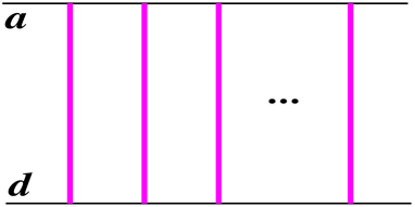
Nevertheless, in MC applications one usually restricts himself with the comparatively simple multi-channel eikonal scheme, where elastic scattering amplitude is described by diagrams of Fig. 1,

Figure 1: General contribution to hadron-hadron scattering amplitude from multiple Pomeron exchanges (vertical thick lines).

corresponding to independent Pomeron exchanges between the two hadrons, and can be expressed via the Pomeron eikonal $\chi_{ad}^{\mathbb{P}}$ as [3]

$$f_{ad}(s,b)=i\sum_{j,l}C_{a(j)}\,C_{d(l)}\left[1-e^{-\lambda_{a(j)}\,\lambda_{d(l)}\,\chi_{ad}^{\mathbb{P}}(Y,b)}\right]\!,$$ (1)

with $Y=\ln s$, $s$ and $b$ being c.m. energy squared and impact parameter for the scattering. A small imaginary part of $\chi_{ad}^{\mathbb{P}}$ can be neglected in the high energy limit. Here $C_{a(j)}$ and $\lambda_{a(j)}$ are correspondingly relative weights and relative strengths of diffraction eigenstates $|a_{j}\rangle$ of hadron $a$ in the multi-component scattering scheme [3]:

$$|a\rangle=\sum_{j}\sqrt{C_{a(j)}}\,|a_{j}\rangle\,,$$ (2)

with $\sum_{j}C_{a(j)}=1$, $\sum_{j}C_{a(j)}\lambda_{a(j)}=1$.

The optical theorem allows one to obtain immediately total hadron-hadron cross section:

$$\sigma^{\rm tot}_{ad}(s)=2\int\!d^{2}b\;{\rm Im}f_{ad}(s,b)=2\sum_{j,l}C_{a(j)}\,C_{d(l)}\int\!d^{2}b\;\left[1-e^{-\lambda_{a(j)}\,\lambda_{d(l)}\,\chi_{ad}^{\mathbb{P}}(Y,b)}\right]\!.$$ (3)

On the other hand, in order to derive partial cross sections for various hadronic final states, one applies the Abramovskii-Gribov-Kancheli (AGK) cutting procedure [11] to obtain asymptotically non-negligible unitarity cuts of the elastic scattering diagrams of Fig. 1. Combining together contributions of cuts of certain topologies, one can identify them with partial contributions of particular final states.

For example, the so-called topological cross sections, corresponding to the interaction being composed of $m\geq 1$ “elementary” particle production processes, are given by the contributions of of graphs in Fig. 2 (left),

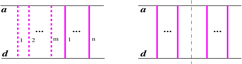
Figure 2: General contribution to multiple production cross section (left) and to the elastic and low mass diffraction cross sections (right). Cut and uncut Pomerons are shown by respectively dashed and solid vertical thick lines; the cut plane is indicated when relevant by the dot-dashed line.

with precisely $m$ Pomerons being cut, and with any number $n$ of uncut ones [3]:

$$\sigma^{(m)}_{ad}(s)=\sum_{n=0}^{\infty}\sum_{j,l}C_{a(j)}\,C_{d(l)}\int\!d^{2}b\;\frac{\left[2\lambda_{a(j)}\,\lambda_{d(l)}\,\chi_{ad}^{\mathbb{P}}(Y,b)\right]^{m}}{m!}\frac{\left[-2\lambda_{a(j)}\,\lambda_{d(l)}\,\chi_{ad}^{\mathbb{P}}(Y,b)\right]^{n}}{n!}$$

$$=\sum_{j,l}C_{a(j)}\,C_{d(l)}\int\!d^{2}b\;\frac{\left[2\lambda_{a(j)}\,\lambda_{d(l)}\,\chi_{ad}^{\mathbb{P}}(Y,b)\right]^{m}}{m!}\;e^{-2\lambda_{a(j)}\,\lambda_{d(l)}\,\chi_{ad}^{\mathbb{P}}(Y,b)}\,.$$ (4)

On the other hand, requiring the cut plane to pass between uncut Pomerons, with at least one on either side of the cut, as shown in Fig. 2 (right), one obtains

$$\sigma^{(0)}_{ad}(s)=\sum_{j,l}C_{a(j)}\,C_{d(l)}\int\!d^{2}b\;\left[1-e^{-\lambda_{a(j)}\,\lambda_{d(l)}\,\chi_{ad}^{\mathbb{P}}(Y,b)}\right]^{2}\!,$$ (5)

which can be further split into elastic and diffraction dissociation cross sections [3]. One can easily verify that the sum of (4) and (5) satisfies the $s$-channel unitarity relation:

$$\sigma^{(0)}_{ad}(s)+\sum_{m=1}^{\infty}\sigma^{(m)}_{ad}(s)=\sigma^{\rm tot}_{ad}(s)\,.$$ (6)

However, the above-described scheme can account only for low mass inelastic excitations of the projectile and target hadrons, where the integration over the masses of those inelastic intermediate states can be performed irrespective the total c. m. energy $s$ for the scattering [3]. To treat high mass diffraction, one has to generalize the scheme, including the contributions of enhanced Pomeron diagrams, i.e. to take Pomeron-Pomeron interactions into account [12, 13, 6, 7, 8]. Moreover, such enhanced diagrams provide important absorptive corrections to the cross sections (3–5) and generate new final states of complicated topologies [13, 7, 8, 14, 15]. 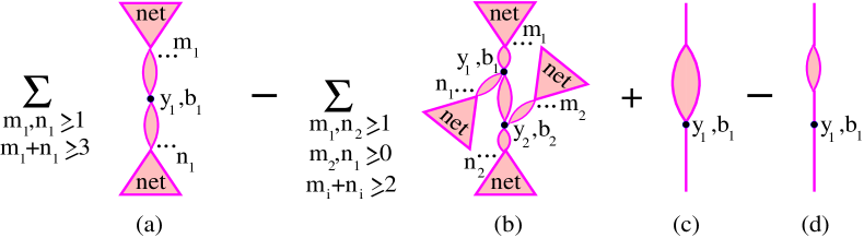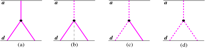For example, cutting the simplest triple-Pomeron diagram of Fig. 3 (a),

Figure 3: Triple-Pomeron contribution to the elastic scattering amplitude (a) and its AGK cuts: high mass diffraction contribution (b), screening correction to one cut Pomeron process (c), and “cut Pomeron fusion” process (d).

one obtains the projectile high mass diffraction contribution of Fig. 3 (b), a screening correction to one cut Pomeron process (Fig. 3 (c)), and a new “cut Pomeron fusion” process of Fig. 3 (d). With increasing energy, more complicated enhanced diagrams, with numerous multi-Pomeron vertices, become important. Thus, to obtain meaningful expressions for the contributions of various hadronic final states, one has to perform a re-summation of the whole series of the corresponding cut diagrams.

A general procedure for the re-summation of enhanced diagram contributions to the elastic scattering amplitude has been proposed in [14]. The goal of the present work is to apply the method for the re-summation of cut diagram contributions and to obtain a full set of the AGK-based unitarity cuts for the considered class of uncut enhanced Pomeron graphs. Mainly, we deal below with diagrams of “net” type, i.e. with arbitrary enhanced diagrams which do not contain Pomeron “loops” (multi-Pomeron vertices connected to each other by two or more Pomerons), although we shall demonstrate how the method can be generalized to include rather general Pomeron loop contributions. An analysis of the structure of final states corresponding to various unitarity cuts and an implementation of the approach in a hadronic MC generator is discussed elsewhere [16].

The paper is organized as follows. In Section 2 we remind the basic results of the earlier works [14, 15] on the re-summation of uncut enhanced diagrams. In Section 3 we analyze unitarity cuts of certain sub-graphs of general net diagrams (so-called “net fans”) and perform a re-summation of the cuts characterized by certain topologies of cut Pomerons. Next, in Section 4 we use those re-summed contributions as building blocks in the construction of the full set of cut non-loop enhanced diagrams, corresponding to the full discontinuity of the elastic scattering contributions of Section 2. Finally, in Section 5 we outline a generalization of the present scheme to include Pomeron loop contributions. We conclude in Section 6.

2 Uncut enhanced diagrams

Taking Pomeron-Pomeron interactions into account, one has to consider multiple exchanges of coupled enhanced graphs, in addition to simple Pomeron exchanges of Fig. 1. The elastic scattering amplitude can still be written in the usual multi-channel eikonal form (c.f. (1)):

$$f_{ad}(s,b)=i\sum_{j,l}C_{a(j)}\,C_{d(l)}\left[1-e^{-\lambda_{a(j)}\,\lambda_{d(l)}\,\chi_{ad}^{\mathbb{P}}(Y,b)+\chi_{ad(jl)}^{{\rm enh}}(Y,b)}\right]\!,$$ (7)

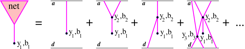
where $\chi_{ad(jl)}^{{\rm enh}}$ stays for the eikonal contribution of irreducible enhanced graphs exchanged between the diffraction eigenstates $|a_{j}\rangle$ and $|d_{l}\rangle$ of hadrons $a$ and $d$. Restricting oneself with non-loop enhanced diagrams, one can express $\chi_{ad(jl)}^{{\rm enh}}$ via the contributions $\chi_{a(j)|d(l)}^{{\rm net}}$ of sub-graphs of certain structure, so-called “net fans”, as shown in Fig. 4 [14, 15].

Figure 4: Irreducible contributions of non-loop enhanced diagrams to elastic scattering amplitude; the vertices $(y_{i},b_{i})$ are coupled to $m_{i}$ projectile and $n_{i}$ target “net fans”, $i=1,2$; $y_{i}$ and $\vec{b}_{i}$ define respectively rapidity and impact parameter positions of multi-Pomeron vertices.

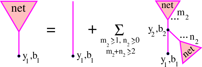
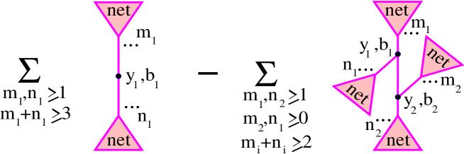
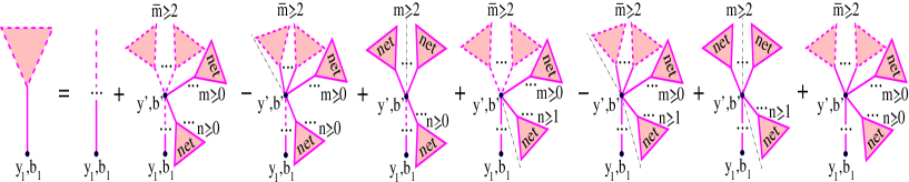
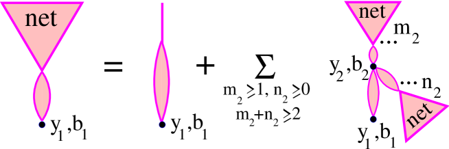
Here the “net fan” contributions $\chi_{a(j)|d(l)}^{{\rm net}}$ are defined by the recursive equation of Fig. 5.

Figure 5: Recursive equation for the “net fan” contribution $\chi_{a(j)|d(l)}^{{\rm net}}(y_{1},\vec{b}_{1}|Y,\vec{b})$; $y_{1}$ and $b_{1}$ are rapidity and impact parameter distances between hadron $a$ and the vertex in the “fan handle”.

In particular, assuming eikonal structure of the vertices for the transition of $m$ into $n$ Pomerons [13]:

$$g_{mn}=G\,\gamma_{\mathbb{P}}^{m+n}\,,$$ (8)

with $r_{3{\mathbb{P}}}=G/(8\pi\gamma_{\mathbb{P}}^{3})$ being the triple-Pomeron constant, the representations of Figs. 4, 5 yield [14, 15]:

$$\chi_{ad(jl)}^{{\rm enh}}(Y,b)=G\int_{0}^{Y}\!dy_{1}\int\!d^{2}b_{1}\left\{(1-e^{-\chi_{a|d}^{{\rm net}}(1)})\,(1-e^{-\chi_{d|a}^{{\rm net}}(1)})-\chi_{a|d}^{{\rm net}}(1)\;\chi_{d|a}^{{\rm net}}(1)\right.$$

$$-G\int_{0}^{y_{1}}\!dy_{2}\int\!d^{2}b_{2}\;\chi_{\mathbb{PP}}^{\mathbb{P}}(y_{1}-y_{2},|\vec{b}_{1}-\vec{b}_{2}|)\;\left[(1-e^{-\chi_{a|d}^{{\rm net}}(1)})\,e^{-\chi_{d|a}^{{\rm net}}(1)}-\chi_{a|d}^{{\rm net}}(1)\right]$$

$$\left.\times\left[(1-e^{-\chi_{d|a}^{{\rm net}}(2)})\,e^{-\chi_{a|d}^{{\rm net}}(2)}-\chi_{d|a}^{{\rm net}}(2)\right]\right\}$$ (9)

$$\chi_{a(j)|d(l)}^{{\rm net}}(y_{1},\vec{b}_{1}|Y,\vec{b})=\lambda_{a(j)}\,\chi_{a\mathbb{P}}^{\mathbb{P}}(y_{1},b_{1})+G\int_{0}^{y_{1}}\!dy_{2}\int\!d^{2}b_{2}\;\chi_{\mathbb{PP}}^{\mathbb{P}}(y_{1}-y_{2},|\vec{b}_{1}-\vec{b}_{2}|)$$

$$\times\left\{(1-e^{-\chi_{a(j)|d(l)}^{{\rm net}}\!(y_{2},\vec{b}_{2}|Y,\vec{b})})\;e^{-\chi_{d(l)|a(j)}^{{\rm net}}\!(Y-y_{2},\vec{b}-\vec{b}_{2}|Y,\vec{b})}-\chi_{a(j)|d(l)}^{{\rm net}}(y_{2},\vec{b}_{2}|Y,\vec{b})\right\}\!,$$ (10)

where $\chi_{a\mathbb{P}}^{\mathbb{P}}(y_{1},b_{1})$ is the eikonal for a Pomeron exchange between hadron $a$ and the vertex $(y_{1},\vec{b}_{1})$, $y_{1}$ and $b_{1}$ being rapidity and impact parameter distances between hadron $a$ and that vertex, whereas the eikonal $\chi_{\mathbb{PP}}^{\mathbb{P}}(y_{1}-y_{2},|\vec{b}_{1}-\vec{b}_{2}|)$ corresponds to a Pomeron exchange between the vertices $(y_{1},\vec{b}_{1})$ and $(y_{2},\vec{b}_{2})$. In (9) we used the abbreviations $\chi_{a|d}^{{\rm net}}(i)\equiv\chi_{a(j)|d(l)}^{{\rm net}}(Y-y_{i},\vec{b}-\vec{b}_{i}|Y,\vec{b})$, $\chi_{d|a}^{{\rm net}}(i)\equiv\chi_{d(l)|a(j)}^{{\rm net}}(y_{i},\vec{b}_{i}|Y,\vec{b})$, $i=1,2$.

The nickname “net fan” for the contribution $\chi_{a(j)|d(l)}^{{\rm net}}(y_{1},\vec{b}_{1}|Y,\vec{b})$ is because the Schwinger-Dyson equation of Fig. 5 generates Pomeron nets exchanged between hadrons $a$ and $d$, starting from a given vertex $(y_{1},\vec{b}_{1})$, some examples shown in Fig. 6,

Figure 6: Some examples of “net fan” diagrams.

and because this equation is formally similar to the usual fan diagram equation. The latter can be recovered setting $n_{2}\equiv 0$ in Fig. 5. In that case (10) reduces to

$$\chi_{a(j)}^{{\rm fan}}(y_{1},{b}_{1})=\lambda_{a(j)}\,\chi_{a\mathbb{P}}^{\mathbb{P}}(y_{1},b_{1})+G\int_{0}^{y_{1}}\!dy_{2}\int\!d^{2}b_{2}\;\chi_{\mathbb{PP}}^{\mathbb{P}}(y_{1}-y_{2},|\vec{b}_{1}-\vec{b}_{2}|)$$

$$\times\left[1-e^{-\chi_{a(j)}^{{\rm fan}}\!(y_{2},{b}_{2})}-\chi_{a(j)}^{{\rm fan}}(y_{2},{b}_{2})\right]\!.$$ (11)

In contrast to the fan contribution $\chi_{a(j)}^{{\rm fan}}$, which can be associated with parton density of a free hadron $a$ [2], the “net fan” equation of Fig. 5 accounts for absorptive corrections due to the re-scattering on the partner hadron $d$ and corresponds to parton momentum and impact parameter distribution which is probed during the interaction [14, 8]. In the following, the Pomeron connected to the initial vertex $(y_{1},\vec{b}_{1})$ in Fig. 5 will be referred to as the “fan handle”.

In the representation of Fig. 4 for enhanced diagram contribution to the elastic scattering amplitude, the first graph in the r.h.s. corresponds to any number $m_{1}\geq 1$ of projectile “net fans” $\chi_{a(j)|d(l)}^{{\rm net}}$ and any number $n_{1}\geq 1$ of target ones $\chi_{d(l)|a(j)}^{{\rm net}}$, $m_{1}+n_{1}\geq 3$, which are coupled together in some “central” vertex, whereas the second graph in the Figure is the double counting correction. Any diagram with $n$ multi-Pomeron vertices is generated $n$ times by the first graph in the r.h.s. of Fig. 4 (as there are $n$ choices for the “central” vertex), from which $(n-1)$ contributions are subtracted by the second graph.

3 Unitarity cuts of “net fans”

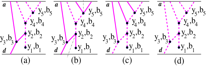
Before considering the cuts of the elastic scattering graphs of Fig. 4, let us apply the AGK cutting procedure to the “net fan” contributions of Fig. 5. It is convenient to separate various unitarity cuts of “net fan” graphs in two classes: in the first sub-set cut Pomerons form fan-like structures, some examples shown in Fig. 7 (a), (b);

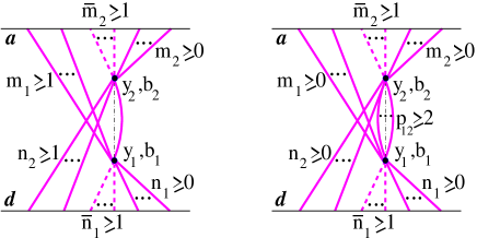
Figure 7: Examples of graphs obtained by cutting the same projectile “net fan” diagram: in the graphs (a) and (b) we have a fan-like structure of cut Pomerons; in the diagrams (c) and (d) the cut Pomeron, exchanged between the vertices ($y_{2},\vec{b}_{2}$) and ($y_{3},\vec{b}_{3}$), is arranged in a zigzag way with respect to the “fan handle”.

in the diagrams of the second kind some cut Pomerons are connected to each other in a zigzag way, such that Pomeron end rapidities are arranged as $y_{1}>y_{2}<y_{3}>...$, see Fig. 7 (c), (d).

Let us consider the first class and obtain separately both the total contribution of fan-like cuts $2\bar{\chi}_{a(j)|d(l)}^{{\rm fan}}$ and the part of it, formed by diagrams with the handle of the fan being uncut, an example shown in Fig. 7 (b), $2\tilde{\chi}_{a(j)|d(l)}^{{\rm fan}}$. Applying AGK cutting rules to the graphs of Fig. 5 and collecting contributions of cuts of desirable structures we obtain for $2\bar{\chi}_{a(j)|d(l)}^{{\rm fan}}-2\tilde{\chi}_{a(j)|d(l)}^{{\rm fan}}$, $2\tilde{\chi}_{a(j)|d(l)}^{{\rm fan}}$ the representations of Figs. 8 and 9,

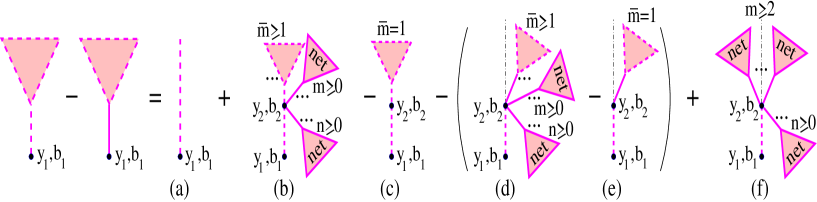
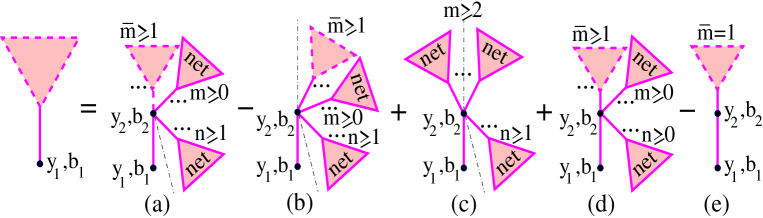
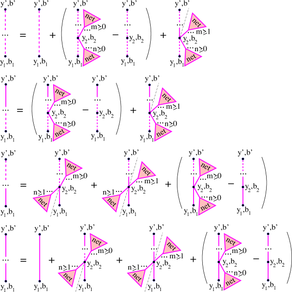
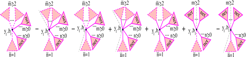
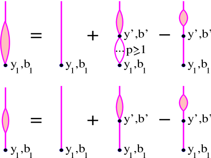
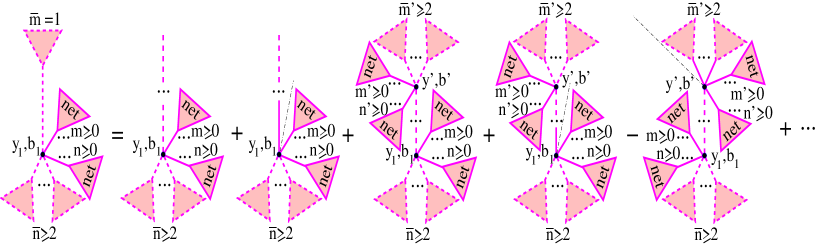
Figure 8: Recursive equation for the contribution $2\bar{\chi}_{a(j)|d(l)}^{{\rm fan}}-2\tilde{\chi}_{a(j)|d(l)}^{{\rm fan}}$ of fan-like cuts of “net fan” diagrams, the handle of the fan being cut.

Figure 9: Recursive equation for the contribution $2\tilde{\chi}_{a(j)|d(l)}^{{\rm fan}}$ of fan-like cuts of “net fan” diagrams, the handle of the fan being uncut.

which gives

$$2\bar{\chi}_{a(j)|d(l)}^{{\rm fan}}(y_{1},\vec{b}_{1}|Y,\vec{b})-2\tilde{\chi}_{a(j)|d(l)}^{{\rm fan}}(y_{1},\vec{b}_{1}|Y,\vec{b})=2\lambda_{a(j)}\,\chi_{a\mathbb{P}}^{\mathbb{P}}(y_{1},b_{1})$$

$$+G\int_{0}^{y_{1}}\!dy_{2}\int\!d^{2}b_{2}\;\chi_{\mathbb{PP}}^{\mathbb{P}}\left\{\left[(e^{2\bar{\chi}_{a|d}^{{\rm fan}}}-1)\>e^{-2\chi_{a|d}^{{\rm net}}-2\chi_{d|a}^{{\rm net}}}-2\bar{\chi}_{a|d}^{{\rm fan}}\right]\right.$$

$$\left.-2\left[(e^{\tilde{\chi}_{a|d}^{{\rm fan}}}-1)\>e^{-\chi_{a|d}^{{\rm net}}-2\chi_{d|a}^{{\rm net}}}-\tilde{\chi}_{a|d}^{{\rm fan}}\right]+(1-e^{-\chi_{a|d}^{{\rm net}}})^{2}\>e^{-2\chi_{d|a}^{{\rm net}}}\right\}$$ (12)

$$2\tilde{\chi}_{a(j)|d(l)}^{{\rm fan}}(y_{1},\vec{b}_{1}|Y,\vec{b})=G\int_{0}^{y_{1}}\!dy_{2}\int\!d^{2}b_{2}\;\chi_{\mathbb{PP}}^{\mathbb{P}}\left\{(1-e^{-\chi_{d|a}^{{\rm net}}})\>e^{-\chi_{d|a}^{{\rm net}}}\left[(e^{2\bar{\chi}_{a|d}^{{\rm fan}}}-1)\>e^{-2\chi_{a|d}^{{\rm net}}}\right.\right.$$

$$\left.\left.-2\,(e^{\tilde{\chi}_{a|d}^{{\rm fan}}}-1)\>e^{-\chi_{a|d}^{{\rm net}}}+(1-e^{-\chi_{a|d}^{{\rm net}}})^{2}\right]+2\left[(e^{\tilde{\chi}_{a|d}^{{\rm fan}}}-1)\>e^{-\chi_{a|d}^{{\rm net}}-\chi_{d|a}^{{\rm net}}}-\tilde{\chi}_{a|d}^{{\rm fan}}\right]\right\}\!.$$ (13)

Here the omitted indices and arguments of the eikonals in the integrands in (12-13) read $\chi_{\mathbb{PP}}^{\mathbb{P}}\equiv\chi_{\mathbb{PP}}^{\mathbb{P}}(y_{1}-y_{2},|\vec{b}_{1}-\vec{b}_{2}|)$, $X_{a|d}\equiv X_{a(j)|d(l)}(y_{2},\vec{b}_{2}|Y,\vec{b})$, $X_{d|a}\equiv X_{d(l)|a(j)}(Y-y_{2},\vec{b}-\vec{b}_{2}|Y,\vec{b})$, $X=\chi^{{\rm net}},\bar{\chi}^{{\rm fan}},\tilde{\chi}^{{\rm fan}}$.

The first diagram in the r.h.s. of Fig. 8 is obtained by cutting the single Pomeron exchanged between hadron $a$ and the vertex $(y_{1},b_{1})$ in the r.h.s. of Fig. 5, whereas the other ones come from cutting the 2nd graph in the r.h.s. of Fig. 5 in such a way that all cut Pomerons are arranged in a fan-like structure and the cut plane passes through the handle Pomeron. In graph (b) the vertex $(y_{2},b_{2})$ couples together $\bar{m}\geq 1$ cut projectile “net fans”, each one characterized by a fan-like structure of cuts, and any numbers $m,n\geq 0$ of uncut projectile and target “net fans”. Here one has to subtract the Pomeron self-coupling contribution ($\bar{m}=1$, $m=n=0$) - graph (c), as well as the contributions of graphs (d) and (e), where in all $\bar{m}$ cut projectile “net fans”, connected to the vertex $(y_{2},b_{2})$, the handle Pomerons remain uncut and all these handle Pomerons and all the $m$ uncut projectile “net fans” are situated on the same side of the cut plane. Finally, in graph (f) the cut plane passes between $m\geq 2$ uncut projectile “net fans”, with at least one remained on either side of the cut.

In the recursive representation of Fig. 9 for the contribution $2\tilde{\chi}_{a(j)|d(l)}^{{\rm fan}}$, the graphs (a), (b), (c) in the r.h.s. of the Figure are similar to the diagrams (b), (d), (f) of Fig. 8 correspondingly, with the difference that the handle of the fan is now uncut. Therefore, there are $n\geq 1$ uncut target “net fans” connected to the vertex $(y_{2},b_{2})$ in such a way that at least one of them is positioned on the opposite side of the cut plane with respect to the handle Pomeron. On the other hand, one has to add graph (d), where the vertex $(y_{2},b_{2})$ couples together $\bar{m}\geq 1$ projectile “net fans”, which are cut in a fan-like way and have their handle Pomerons uncut and positioned on the same side of the cut plane, together with any numbers $m\geq 0$ of projectile and $n\geq 0$ of target uncut “net fans”, such that the vertex remains uncut. Here one has to subtract the Pomeron self-coupling ($\bar{m}=1$, $m=n=0$) – graph (e).

Adding (13) to (12), we obtain

$$2\bar{\chi}_{a(j)|d(l)}^{{\rm fan}}(y_{1},\vec{b}_{1}|Y,\vec{b})=2\lambda_{a(j)}\,\chi_{a\mathbb{P}}^{\mathbb{P}}(y_{1},b_{1})$$

$$+G\int_{0}^{y_{1}}\!\!dy_{2}\int\!\!d^{2}b_{2}\;\chi_{\mathbb{PP}}^{\mathbb{P}}\,\left\{\left[(e^{2\bar{\chi}_{a|d}^{{\rm fan}}}-1)\,e^{-2\chi_{a|d}^{{\rm net}}}+(1-e^{-\chi_{a|d}^{{\rm net}}})^{2}\right]e^{-\chi_{d|a}^{{\rm net}}}-2\bar{\chi}_{a|d}^{{\rm fan}}\right\}\!,\!\!$$ (14)

with the solution (c.f. (10))

$$\bar{\chi}_{a(j)|d(l)}^{{\rm fan}}(y_{1},\vec{b}_{1}|Y,\vec{b})=\chi_{a(j)|d(l)}^{{\rm net}}(y_{1},\vec{b}_{1}|Y,\vec{b}).$$ (15)

To investigate zigzag-like cuts of “net fan” graphs, the examples shown in Fig. 7 (c) and (d), we introduce $k$-th order cut “net fan” contributions $2\bar{\chi}_{a(j)|d(l)}^{{\rm net}(k)}$, $k\geq 2$, which in addition to the above-considered fan-like cut diagrams contain also ones with up to $k$ cut Pomerons connected to each other in a zigzag way, i.e., with Pomeron end rapidities being arranged as $y_{1}>y_{2}<...>y_{k+1}$. For example, the graphs of Fig. 7 (c) and (d) belong correspondingly to the 2nd and 3rd order cut “net fan” contributions. As before, we consider two subsamples of the diagrams, with the handle Pomerons being cut, $2\bar{\chi}_{a(j)|d(l)}^{{\rm net}(k)}-2\tilde{\chi}_{a(j)|d(l)}^{{\rm net}(k)}$, and uncut, $2\tilde{\chi}_{a(j)|d(l)}^{{\rm net}(k)}$, which leads us to the recursive equations of Figs. 10 and 11 respectively.

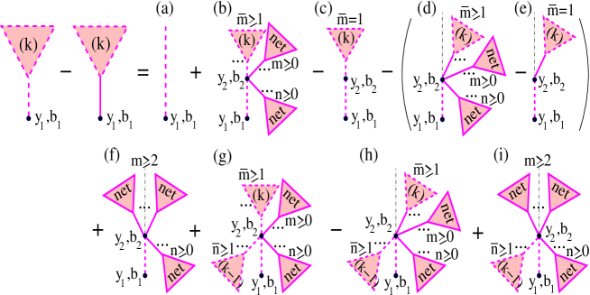
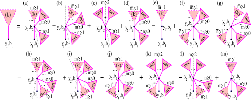
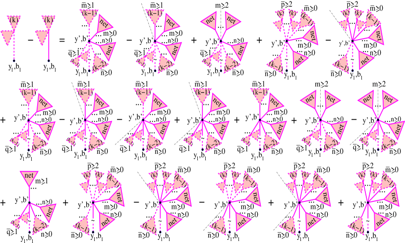
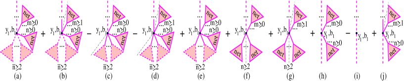
Figure 10: Recursive equation for the $k$-th order cut “net-fan” contribution $2\bar{\chi}_{a(j)|d(l)}^{\rm{net}(k)}-2\tilde{\chi}_{a(j)|d(l)}^{\rm{net}(k)}$ with cut “handle”.

Figure 11: Recursive equation for the $k$-th order cut “net-fan” contribution $2\tilde{\chi}_{a(j)|d(l)}^{\rm{net}(k)}$ with uncut “handle”.

Compared to the ones of Figs. 8 and 9, they contain additional graphs, Fig. 10 (g)-(i) and Fig. 11 (f)-(m), where the vertex $(y_{2},\vec{b}_{2})$ is coupled to $\bar{n}\geq 1$ cut target “net fans” of $(k-1)$-th order (we set $\bar{\chi}_{a(j)|d(l)}^{{\rm net}(1)}\equiv\bar{\chi}_{a(j)|d(l)}^{{\rm fan}}$, $\tilde{\chi}_{a(j)|d(l)}^{{\rm net}(1)}\equiv\tilde{\chi}_{a(j)|d(l)}^{{\rm fan}}$). Thus, we obtain

$$2\bar{\chi}_{a(j)|d(l)}^{{\rm net}(k)}(y_{1},\vec{b}_{1}|Y,\vec{b})-2\tilde{\chi}_{a(j)|d(l)}^{{\rm net}(k)}(y_{1},\vec{b}_{1}|Y,\vec{b})=2\lambda_{a(j)}\,\chi_{a\mathbb{P}}^{\mathbb{P}}(y_{1},b_{1})$$

$$+G\int_{0}^{y_{1}}\!dy_{2}\int\!d^{2}b_{2}\;\chi_{\mathbb{PP}}^{\mathbb{P}}\,\left\{\left[(e^{2\bar{\chi}_{a|d}^{{\rm net}(k)}}-1)\>e^{-2\chi_{a|d}^{{\rm net}}-2\chi_{d|a}^{{\rm net}}}-2\bar{\chi}_{a|d}^{{\rm net}(k)}\right]\right.$$

$$-2\left[(e^{\tilde{\chi}_{a|d}^{{\rm net}(k)}}-1)\>e^{-\chi_{a|d}^{{\rm net}}-2\chi_{d|a}^{{\rm net}}}-\tilde{\chi}_{a|d}^{{\rm net}(k)}\right]+(1-e^{-\chi_{a|d}^{{\rm net}}})^{2}\>e^{-2\chi_{d|a}^{{\rm net}}}$$

$$\left.+\left[(e^{2\bar{\chi}_{a|d}^{{\rm net}(k)}}-1)\>e^{-2\chi_{a|d}^{{\rm net}}}-2(e^{\tilde{\chi}_{a|d}^{{\rm net}(k)}}-1)\>e^{-\chi_{a|d}^{{\rm net}}}+(1-e^{-\chi_{a|d}^{{\rm net}}})^{2}\right]\,(e^{2\bar{\chi}_{d|a}^{{\rm net}(k-1)}}-1)\>e^{-2\chi_{d|a}^{{\rm net}}}\right\}$$ (16)

$$2\tilde{\chi}_{a(j)|d(l)}^{{\rm net}(k)}(y_{1},\vec{b}_{1}|Y,\vec{b})=G\int_{0}^{y_{1}}\!dy_{2}\int\!d^{2}b_{2}\;\chi_{\mathbb{PP}}^{\mathbb{P}}\left\{(1-e^{-\chi_{d|a}^{{\rm net}}})\>e^{-\chi_{d|a}^{{\rm net}}}\left[(e^{2\bar{\chi}_{a|d}^{{\rm net}(k)}}-1)\>e^{-2\chi_{a|d}^{{\rm net}}}\right.\right.$$

$$-\left.2\,(e^{\tilde{\chi}_{a|d}^{{\rm net}(k)}}-1)\>e^{-\chi_{a|d}^{{\rm net}}}+(1-e^{-\chi_{a|d}^{{\rm net}}})^{2}\right]+2\left[(e^{\tilde{\chi}_{a|d}^{{\rm net}(k)}}-1)\>e^{-\chi_{a|d}^{{\rm net}}-\chi_{d|a}^{{\rm net}}}-\tilde{\chi}_{a|d}^{{\rm net}(k)}\right]$$

$$-\left[(e^{2\bar{\chi}_{a|d}^{{\rm net}(k)}}-1)\>e^{-2\chi_{a|d}^{{\rm net}}}-2(e^{\tilde{\chi}_{a|d}^{{\rm net}(k)}}-1)\>e^{-\chi_{a|d}^{{\rm net}}}+(1-e^{-\chi_{a|d}^{{\rm net}}})^{2}\right]\,(e^{2\bar{\chi}_{d|a}^{{\rm net}(k-1)}}-1)\>e^{-2\chi_{d|a}^{{\rm net}}}$$

$$+\left.2\left[(e^{2\bar{\chi}_{a|d}^{{\rm net}(k)}}-1)\,e^{-2\chi_{a|d}^{{\rm net}}}+(1-e^{-\chi_{a|d}^{{\rm net}}})^{2}-2\,(1-e^{-\chi_{a|d}^{{\rm net}}})\right]\,(e^{\tilde{\chi}_{d|a}^{{\rm net}(k-1)}}-1)\>e^{-\chi_{d|a}^{{\rm net}}}\right\}\!.$$ (17)

Adding (16) to (17), we obtain

$$2\bar{\chi}_{a(j)|d(l)}^{{\rm net}(k)}(y_{1},\vec{b}_{1}|Y,\vec{b})=2\lambda_{a(j)}\,\chi_{a\mathbb{P}}^{\mathbb{P}}(y_{1},b_{1})$$

$$+G\int_{0}^{y_{1}}\!\!dy_{2}\int\!\!d^{2}b_{2}\;\chi_{\mathbb{PP}}^{\mathbb{P}}\,\left\{\left[(e^{2\bar{\chi}_{a|d}^{{\rm net}(k)}}-1)\,e^{-2\chi_{a|d}^{{\rm net}}}+(1-e^{-\chi_{a|d}^{{\rm net}}})^{2}\right]e^{-\chi_{d|a}^{{\rm net}}}-2\bar{\chi}_{a|d}^{{\rm net}(k)}\right.$$

$$+\left.2\left[(e^{2\bar{\chi}_{a|d}^{{\rm net}(k)}}-1)\,e^{-2\chi_{a|d}^{{\rm net}}}+(1-e^{-\chi_{a|d}^{{\rm net}}})^{2}-2\,(1-e^{-\chi_{a|d}^{{\rm net}}})\right]\,(e^{\tilde{\chi}_{d|a}^{{\rm net}(k-1)}}-1)\>e^{-\chi_{d|a}^{{\rm net}}}\right\}\!,$$ (18)

with the solution (c.f. (10))

$$\bar{\chi}_{a(j)|d(l)}^{{\rm net}(k)}(y_{1},\vec{b}_{1}|Y,\vec{b})=\chi_{a(j)|d(l)}^{{\rm net}}(y_{1},\vec{b}_{1}|Y,\vec{b})\,.$$ (19)

Thus, for the summary contribution of all cuts of “net fan” graphs of Fig. 4 we obtain $2\bar{\chi}_{a(j)|d(l)}^{{\rm net}}\equiv\lim_{k\rightarrow\infty}2\bar{\chi}_{a(j)|d(l)}^{{\rm net}(k)}=\chi_{a(j)|d(l)}^{{\rm net}}$, as it should be. On the other hand, contributions of various zigzag-like cuts precisely cancel each other

$$2\bar{\chi}_{a(j)|d(l)}^{{\rm zz}(k)}\equiv 2\bar{\chi}_{a(j)|d(l)}^{{\rm net}(k)}-2\bar{\chi}_{a|d}^{{\rm net}(k-1)}=0$$ (20)

$$2\bar{\chi}_{a(j)|d(l)}^{{\rm zz}}\equiv 2\bar{\chi}_{a(j)|d(l)}^{{\rm net}}-2\bar{\chi}_{a(j)|d(l)}^{{\rm fan}}=\sum_{k=2}^{\infty}2\bar{\chi}_{a(j)|d(l)}^{{\rm zz}(k)}=0.$$ (21)

Making use of (19), we can re-write (16) as

$$2\left[\bar{\chi}_{a(j)|d(l)}^{{\rm net}(k)}(y_{1},\vec{b}_{1}|Y,\vec{b})-\tilde{\chi}_{a(j)|d(l)}^{{\rm net}(k)}(y_{1},\vec{b}_{1}|Y,\vec{b})\right]=2\lambda_{a(j)}\,\chi_{a\mathbb{P}}^{\mathbb{P}}(y_{1},b_{1})$$

$$+2G\int_{0}^{y_{1}}\!dy_{2}\int\!d^{2}b_{2}\;\chi_{\mathbb{PP}}^{\mathbb{P}}\,\left\{1-e^{-\left[\bar{\chi}_{a|d}^{{\rm net}(k)}-\tilde{\chi}_{a|d}^{{\rm net}(k)}\right]}-\left[\bar{\chi}_{a|d}^{{\rm net}(k)}-\tilde{\chi}_{a|d}^{{\rm net}(k)}\right]\right\}$$ (22)

and obtain (c.f. (11))

$$\bar{\chi}_{a(j)|d(l)}^{{\rm net}(k)}(y_{1},\vec{b}_{1}|Y,\vec{b})-\tilde{\chi}_{a(j)|d(l)}^{{\rm net}(k)}(y_{1},\vec{b}_{1}|Y,\vec{b})=\chi_{a(j)}^{{\rm fan}}(y_{1},{b}_{1})\,,\;\;\;\;k\geq 2,$$ (23)

i.e. the summary contribution of all AGK cuts of “net fan” graphs, with the cut plane passing through the handle Pomeron, satisfies the usual fan diagram equation (11), being independent on re-scatterings on the partner hadron.

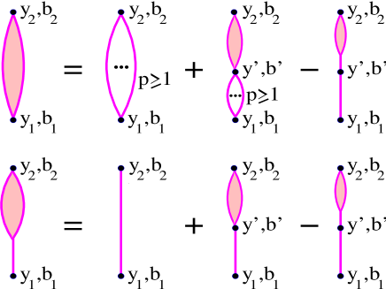
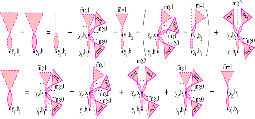
One can obtain an alternative representation for $\bar{\chi}_{a(j)|d(l)}^{{\rm fan}}$, $\tilde{\chi}_{a(j)|d(l)}^{{\rm fan}}$, as shown in Figs. 12 and 13,

Figure 12: Alternative representation for the fan-like cut contribution $2\bar{\chi}_{a(j)|d(l)}^{{\rm fan}}-2\tilde{\chi}_{a(j)|d(l)}^{{\rm fan}}$, with the handle Pomeron being cut. Each broken Pomeron line denotes a $t$-channel sequence of Pomerons which are separated by vertices connected to uncut projectile and target “net fans”.

Figure 13: Alternative representation for the fan-like cut contribution $2\tilde{\chi}_{a(j)|d(l)}^{{\rm fan}}$, with the handle Pomeron being uncut. The broken Pomeron lines have the same meaning as in Fig. 12.

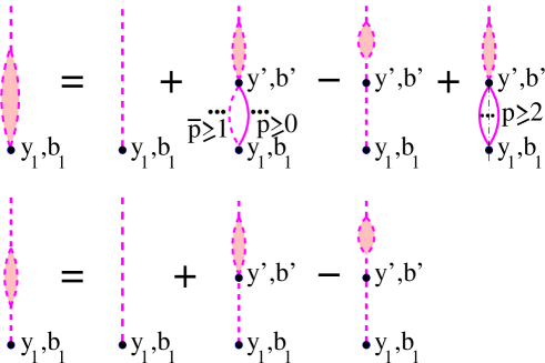
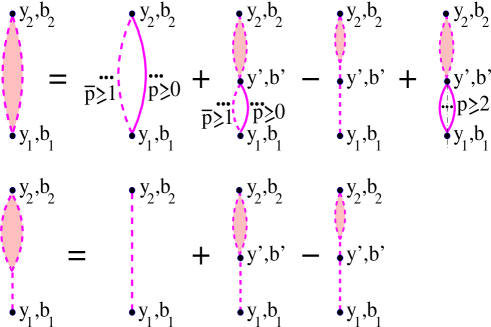
applying (12-13) (correspondingly Figs. 8 and 9) recursively to generate any number of vertices, connected to uncut projectile and target “net fans”, along the handle of the fan. The broken Pomeron lines in Figs. 12 and 13 correspond to $t$-channel sequences of cut and uncut Pomerons, which are separated by vertices connected to uncut projectile and target “net fans”; the corresponding contributions are defined via recursive representations of Fig. 14.

Figure 14: Recursive equations in the Figure generate $t$-channel sequences of cut and uncut Pomerons, which are separated by multi-Pomeron vertices, each one being connected to at least one uncut projectile or target “net fan”.

In particular, the contributions $2\chi_{a(j)|d(l)}^{\mathbb{P}_{{\rm cc}}}$ and $2\chi_{a(j)|d(l)}^{\mathbb{P}_{{\rm uc}}}$ of the first graphs in the r.h.s. of Figs. 12 and 13 respectively (the index ${\mathbb{P}_{xy}}$ indicates whether the downmost (uppermost) Pomeron in the sequence is cut, $x={\rm c}$ ($y={\rm c}$), or uncut, $x={\rm u}$ ($y={\rm u}$)) are defined as (c.f. (12-13))

$$2\chi_{a(j)|d(l)}^{\mathbb{P}_{{\rm cc}}}(y_{1},\vec{b}_{1}|Y,\vec{b})=2\lambda_{a(j)}\,\chi_{a\mathbb{P}}^{\mathbb{P}}(y_{1},b_{1})+2G\int_{0}^{y_{1}}\!dy_{2}\int\!d^{2}b_{2}\;\chi_{\mathbb{PP}}^{\mathbb{P}}$$

$$\times\left[(e^{-2\chi_{a|d}^{{\rm net}}-2\chi_{d|a}^{{\rm net}}}-1)\,(\chi_{a|d}^{\mathbb{P}_{{\rm cc}}}+\chi_{a|d}^{\mathbb{P}_{{\rm uc}}})-(e^{-\chi_{a|d}^{{\rm net}}-2\chi_{d|a}^{{\rm net}}}-1)\,\chi_{a|d}^{\mathbb{P}_{{\rm uc}}}\right]$$ (24)

$$2\chi_{a(j)|d(l)}^{\mathbb{P}_{{\rm uc}}}(y_{1},\vec{b}_{1}|Y,\vec{b})=2G\int_{0}^{y_{1}}\!dy_{2}\int\!d^{2}b_{2}\;\chi_{\mathbb{PP}}^{\mathbb{P}}$$

$$\times\left[(1-e^{-\chi_{d|a}^{{\rm net}}})\,e^{-2\chi_{a|d}^{{\rm net}}-\chi_{d|a}^{{\rm net}}}\,(\chi_{a|d}^{\mathbb{P}_{{\rm cc}}}+\chi_{a|d}^{\mathbb{P}_{{\rm uc}}})+(e^{-\chi_{a|d}^{{\rm net}}-2\chi_{d|a}^{{\rm net}}}-1)\,\chi_{a|d}^{\mathbb{P}_{{\rm uc}}}\right]\!.$$ (25)

Similarly, we can obtain a recursive representation for $k$-th order zigzag-like cut “net fans” $2\bar{\chi}_{a(j)|d(l)}^{{\rm zz}(k)}\equiv 2\bar{\chi}_{a(j)|d(l)}^{{\rm net}(k)}-2\bar{\chi}_{a(j)|d(l)}^{{\rm net}(k-1)}$, $2\tilde{\chi}_{a(j)|d(l)}^{{\rm zz}(k)}\equiv 2\tilde{\chi}_{a(j)|d(l)}^{{\rm net}(k)}-2\tilde{\chi}_{a(j)|d(l)}^{{\rm net}(k-1)}$, applying recursively the relations (16-17) (Figs. 10 and 11) to generate any number of intermediate vertices along the handle Pomeron, which are connected to uncut and $(k-1)$-th order cut projectile and target “net fans”, until we end up with the vertex $(y^{\prime},\vec{b}^{\prime})$, which either couples together $\bar{p}\geq 2$ $k$-th order projectile zigzag-like cut contributions and any numbers of uncut and $(k-1)$-th order cut projectile and target “net fans”, or is coupled to $\bar{q}\geq 1$ $(k-1)$-th order target zigzag-like cut contributions (in addition, to any numbers of uncut and $(k-2)$-th order cut target “net fans”) and to uncut and $(k-1)$-th order cut projectile “net fans”. The corresponding relation for $2\bar{\chi}_{a(j)|d(l)}^{{\rm zz}(k)}-2\tilde{\chi}_{a(j)|d(l)}^{{\rm zz}(k)}$ is shown in Fig. 15,

Figure 15: Recursive equation for the contribution $2\bar{\chi}_{a(j)|d(l)}^{{\rm zz}(k)}-2\tilde{\chi}_{a(j)|d(l)}^{{\rm zz}(k)}$ of zigzag-like cuts of “net-fan” diagrams, the handle Pomeron being cut. The broken Pomeron lines between the vertices $(y_{1},\vec{b}_{1})$ and $(y^{\prime},\vec{b}^{\prime})$ correspond here to $t$-channel sequences of cut and uncut Pomerons, which are separated by multi-Pomeron vertices connected to uncut and $(k-1)$-th order cut projectile and target “net fans”.

the one for $2\tilde{\chi}_{a(j)|d(l)}^{{\rm zz}(k)}$ looks similarly (c.f. Figs. 12 and 13).

4 Cut enhanced diagrams

We are going to derive the complete set of cut diagrams corresponding to $s$-channel discontinuity of elastic scattering contributions of Fig. 4. Let us start with cut graphs characterized by a tree-like structure of cut Pomerons, which can be constructed coupling any numbers $\bar{m},\bar{n}$ of fan-like cut projectile and target “net fans” in one vertex.

First we consider the case of $\bar{m},\bar{n}\neq 1$, which leads us to the set of graphs of Fig. 16,

Figure 16: Tree-like cut enhanced diagrams. The vertex $(y_{1},\vec{b}_{1})$ couples together $\bar{m}$ projectile and $\bar{n}$ target fan-like cut “net fans”; $\bar{m},\bar{n}\neq 1$.

where we do not have any double counting of the same contributions. For example, the graphs Fig. 16 (a)-(e) have a single vertex $(y_{1},\vec{b}_{1})$, which couples together $\bar{m}\geq 2$ projectile and $\bar{n}\geq 2$ target fan-like cut “net fans”. Correspondingly, different structures of cut “net fans” and different topologies of the uncut ones result in different diagrams. For the combined contribution of all the graphs of Fig. 16 we obtain, using (15),

$$2\bar{\chi}_{ad(jl)}^{{\rm tree(1)}}(Y,b)=2G\int_{0}^{Y}\!dy_{1}\int\!d^{2}b_{1}\left\{(1-e^{-\chi_{a|d}^{{\rm net}}}-\chi_{a|d}^{{\rm net}}\>e^{-2\chi_{a|d}^{{\rm net}}})\;(1-e^{-\chi_{d|a}^{{\rm net}}}-\chi_{d|a}^{{\rm net}}\>e^{-2\chi_{d|a}^{{\rm net}}})\right.$$

$$+\left.\chi_{a|d}^{{\rm net}}\;e^{-2\chi_{a|d}^{{\rm net}}-\chi_{d|a}^{{\rm net}}}\;(e^{\tilde{\chi}_{d|a}^{{\rm fan}}}-1-\tilde{\chi}_{d|a}^{{\rm fan}})+\chi_{d|a}^{{\rm net}}\;e^{-\chi_{a|d}^{{\rm net}}-2\chi_{d|a}^{{\rm net}}}\;(e^{\tilde{\chi}_{a|d}^{{\rm fan}}}-1-\tilde{\chi}_{a|d}^{{\rm fan}})\right\}\!,$$ (26)

where we use the abbreviations $X_{a|d}\equiv X_{a(j)|d(l)}(Y-y_{1},\vec{b}-\vec{b}_{1}|Y,\vec{b})$, $X_{d|a}\equiv X_{d(l)|a(j)}(y_{1},\vec{b}_{1}|Y,\vec{b})$, $X=\chi^{{\rm net}}$, $\tilde{\chi}^{{\rm fan}}$.

Now we come to the case of $\bar{m}\neq 1$ and $\bar{n}=1$, which results in the diagrams of Fig. 17.

Figure 17: The same as in Fig. 16 for $\bar{m}\neq 1$ and $\bar{n}=1$.

Similarly to the above, we obtain

$$2\bar{\chi}_{ad(jl)}^{{\rm tree(2)}}(Y,b)=2G\int_{0}^{Y}\!dy_{1}\int\!d^{2}b_{1}\left\{(1-e^{-\chi_{a|d}^{{\rm net}}}-\chi_{a|d}^{{\rm net}}\>e^{-2\chi_{a|d}^{{\rm net}}})\;(\chi_{d|a}^{{\rm net}}\>e^{-2\chi_{d|a}^{{\rm net}}}-\tilde{\chi}_{d|a}^{{\rm fan}}\>e^{-\chi_{d|a}^{{\rm net}}})\right.$$

$$\left.-\chi_{d|a}^{{\rm net}}\;e^{-\chi_{a|d}^{{\rm net}}-2\chi_{d|a}^{{\rm net}}}\;(e^{\tilde{\chi}_{a|d}^{{\rm fan}}}-1-\tilde{\chi}_{a|d}^{{\rm fan}})\right\}\!.$$ (27)

Finally we consider the case of $\bar{n}\neq 1$ and $\bar{m}=1$, which can be obtained reversing the graphs of Fig. 17 upside-down. There we have to correct for double counting of the same contributions. For example, considering the first diagram of Fig. 17 being reversed upside-down and expanding its projectile fan-like cut “net fan” using the relations of Figs. 12 and 13, we obtain the set of graphs of Fig. 18.

Figure 18: Cut diagram on the l.h.s. can be expanded as shown in the picture.

Clearly, the third diagram in the r.h.s. of Fig. 18, being symmetric with respect to the projectile and the target, will appear in a similar expansion of the first graph of Fig. 17. On the other hand, all the other graphs in the r.h.s. of Fig. 18, except the first two, find their duplicates in the expansions of other diagrams of Fig. 17. Thus, the only new contributions are the ones of Fig. 19 (a)-(g).

Figure 19: Additional tree-like cut diagrams, not included in Figs. 16, 17.

In addition, we have to include the graphs (h)-(j) of the Figure, which correspond to a $t$-channel sequence of $l\geq 2$ cut and uncut Pomerons which are separated by vertices connected to uncut projectile and target “net fans”, with the downmost and the uppermost Pomerons in the sequence being cut. The contribution of the graphs of Fig. 19 is

$$2\bar{\chi}_{ad(jl)}^{{\rm tree(3)}}\!(Y,b)=2G\int_{0}^{Y}\!dy_{1}\int\!d^{2}b_{1}\left\{\left[(\chi_{a|d}^{\mathbb{P}_{{\rm cc}}}+\chi_{a|d}^{\mathbb{P}_{{\rm uc}}})\;e^{-2\chi_{a|d}^{{\rm net}}}-\chi_{a|d}^{\mathbb{P}_{{\rm uc}}}\;e^{-\chi_{a|d}^{{\rm net}}}\right]\right.$$

$$\times\;(1-e^{-\chi_{d|a}^{{\rm net}}}-\chi_{d|a}^{{\rm net}}\>e^{-2\chi_{d|a}^{{\rm net}}})-(\chi_{a|d}^{\mathbb{P}_{{\rm cc}}}+\chi_{a|d}^{\mathbb{P}_{{\rm uc}}})\;(e^{\tilde{\chi}_{d|a}^{{\rm fan}}}-1-\tilde{\chi}_{d|a}^{{\rm fan}})\>e^{-2\chi_{a|d}^{{\rm net}}-\chi_{d|a}^{{\rm net}}}$$

$$+\left.\lambda_{d(l)}\,\chi_{d\mathbb{P}}^{\mathbb{P}}(y_{1},b_{1})\left[\chi_{a|d}^{\mathbb{P}_{{\rm cc}}}\>(e^{-2\chi_{a|d}^{{\rm net}}-2\chi_{d|a}^{{\rm net}}}-1)-\chi_{a|d}^{\mathbb{P}_{{\rm uc}}}\>e^{-\chi_{a|d}^{{\rm net}}-2\chi_{d|a}^{{\rm net}}}\>(1-e^{-\chi_{a|d}^{{\rm net}}})\right]\right\}\!.$$ (28)

Adding (26-28) together and using (10), (13), (15), (24-25), we can obtain

$$2\bar{\chi}_{ad(jl)}^{{\rm tree}}(Y,b)=\sum_{i=1}^{3}2\bar{\chi}_{ad(jl)}^{{\rm tree(i)}}(Y,b)=2G\int_{0}^{Y}\!dy_{1}\int\!d^{2}b_{1}\left\{(1-e^{-\chi_{a|d}^{{\rm net}}})\,(1-e^{-\chi_{d|a}^{{\rm net}}})-\chi_{a|d}^{{\rm net}}\>\chi_{d|a}^{{\rm net}}\right.$$

$$-\left.\left[(1-e^{-\chi_{d|a}^{{\rm net}}})\;e^{-\chi_{a|d}^{{\rm net}}}-\chi_{d|a}^{{\rm net}}\right](\chi_{a|d}^{{\rm net}}-\lambda_{a(j)}\,\chi_{a\mathbb{P}}^{\mathbb{P}}(Y-y_{1},|\vec{b}-\vec{b}_{1}|)\right\}=2\chi_{ad(jl)}^{{\rm enh}}(Y,b)\,.$$ (29)

However, the unitarity requires the sum of all the cuts of the diagrams of Fig. 4 to be equal to twice the imaginary part of the elastic scattering contribution, i.e. to $2\chi_{ad(jl)}^{{\rm enh}}$. Thus, the contributions of all cuts of non-tree (zigzag) type should precisely cancel each other. To verify that, we can construct the complete set of corresponding cut diagrams replacing in Figs. 16 and 17 some contributions $\bar{\chi}_{a(j)|d(l)}^{{\rm fan}}$ and $\tilde{\chi}_{a(j)|d(l)}^{{\rm fan}}$ ($\bar{\chi}_{d(l)|a(j)}^{{\rm fan}}$ and $\tilde{\chi}_{d(l)|a(j)}^{{\rm fan}}$ ) by $\bar{\chi}_{a(j)|d(l)}^{{\rm zz(k)}}$ and $\tilde{\chi}_{a(j)|d(l)}^{{\rm zz(k)}}$ ($\bar{\chi}_{d(l)|a(j)}^{{\rm zz(k)}}$ and $\tilde{\chi}_{d(l)|a(j)}^{{\rm zz(k)}}$), whereas the others – by $\bar{\chi}_{a(j)|d(l)}^{{\rm net(k-1)}}$ and $\tilde{\chi}_{a(j)|d(l)}^{{\rm net(k-1)}}$ ($\bar{\chi}_{d(l)|a(j)}^{{\rm net(k-1)}}$ and $\tilde{\chi}_{d(l)|a(j)}^{{\rm net(k-1)}}$), starting from $k=2$, etc. Using the representation of Fig. 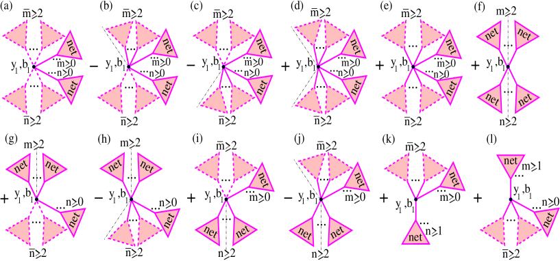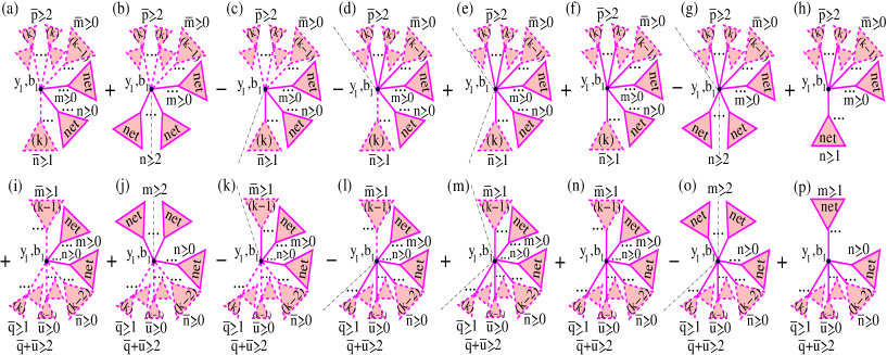15 for $2\bar{\chi}_{a(j)|d(l)}^{{\rm zz}(k)}-2\tilde{\chi}_{a(j)|d(l)}^{{\rm zz}(k)}$ (similarly for $2\tilde{\chi}_{a(j)|d(l)}^{{\rm zz}(k)}$) to correct for double counts in the same way as above for the tree-like cut diagrams, we obtain the set of graphs of Fig. 20.

Figure 20: Cut enhanced diagrams with non-tree-like topology of cut Pomerons.

There, the diagrams (a)–(c) contain $\bar{p}\geq 2$ $k$-th order projectile zigzag-like cut “net fans”; this gives a factor $(e^{2\bar{\chi}_{a(j)|d(l)}^{{\rm zz}(k)}}-1-2\bar{\chi}_{a(j)|d(l)}^{{\rm zz}(k)})$, which is equal zero due to (20). Similarly, the graphs (i)–(k) have $\bar{q}\geq 1$ $k$-th order target zigzag-like cut “net fans”, which gives $(e^{2\bar{\chi}_{d(l)|a(j)}^{{\rm zz}(k)}}-1)=0$. The contributions of the graphs (e) and (f) are equal up to a sign and cancel each other; the same applies to the diagrams (m) and (n). Finally, the graphs (d), (g), (h) give together

$$G\int_{0}^{Y}\!\!dy_{1}\!\int\!d^{2}b_{1}\;(e^{\tilde{\chi}_{a|d}^{{\rm zz}(k)}}-1-\tilde{\chi}_{a|d}^{{\rm zz}(k)})\;e^{\tilde{\chi}_{a|d}^{{\rm net}(k-1)}-\chi_{a|d}^{{\rm net}}}$$

$$\times\left[-(e^{2\bar{\chi}_{d|a}^{{\rm net}(k)}}-1)\;e^{-2\chi_{d|a}^{{\rm net}}}-(1-e^{-\chi_{d|a}^{{\rm net}}})^{2}+2(1-e^{-\chi_{d|a}^{{\rm net}}})\right]\!,$$ (30)

where the expression in the square brackets vanishes due to (19). Similarly one demonstrates the cancellation for the graphs (l), (o), and (p). This completes the proof of the $s$-channel unitarity of the approach. It is worth stressing that we obtained a cancellation for the contributions of non-tree type cut diagrams of Fig. 20 to the total cross section, not to inclusive particle spectra; such graphs have to be taken into consideration in inelastic event generation procedures.

It is noteworthy that the $s$-channel unitarity is still violated in the described scheme in certain parts of the kinematic space, which is the price for neglecting Pomeron loop contributions. For example, one obtains here a negative contribution for double high mass diffraction (central rapidity gap) cross section $\sigma_{ad}^{\rm DD}$. Indeed, dominant contribution to the process comes from hadron-hadron scattering at relatively large impact parameters, where the RGS probability is not too small, and, due to the smallness of the triple-Pomeron coupling $r_{3{\mathbb{P}}}$, is given by the graphs of Fig. 21 (left),

Figure 21: Lowest order contributions to the double high mass diffraction cross section: net-like diagrams (left) and loop graphs (right).

with only two multi-Pomeron vertices. Thus, for $\sigma_{ad}^{\rm DD}$ one obtains

$$\sigma_{ad}^{\rm DD}(s,y_{1},y_{2})\simeq-\frac{G}{2}\sum_{j,l}C_{a(j)}\,C_{d(l)}\int\!d^{2}b\,d^{2}b_{1}\,d^{2}b_{1}\;\chi_{\mathbb{PP}}^{\mathbb{P}}(y_{2}-y_{1},|\vec{b}_{2}-\vec{b}_{1}|)$$

$$\times(1-e^{-2\lambda_{a(j)}\,\chi_{a\mathbb{P}}^{\mathbb{P}}(Y-y_{2},|\vec{b}-\vec{b}_{2}|)})\;(1-e^{-\lambda_{d(l)}\,\chi_{d\mathbb{P}}^{\mathbb{P}}(y_{2},b_{2})})\;e^{-\lambda_{d(l)}\,\chi_{d\mathbb{P}}^{\mathbb{P}}(y_{2},b_{2})}\;(1-e^{-2\lambda_{d(l)}\,\chi_{d\mathbb{P}}^{\mathbb{P}}(y_{1},b_{1})})$$

$$\times(1-e^{-\lambda_{a(j)}\,\chi_{a\mathbb{P}}^{\mathbb{P}}(Y-y_{1},|\vec{b}-\vec{b}_{1}|)})\;e^{-\lambda_{a(j)}\,\chi_{a\mathbb{P}}^{\mathbb{P}}(Y-y_{1},|\vec{b}-\vec{b}_{1}|)}\;S^{\rm RG}_{ad(jl)}(Y,b,y_{1},y_{2})\,,$$ (31)

where $S^{\rm RG}_{ad(jl)}(Y,b,y_{1},y_{2})$ is the (positively defined) RGS factor, i.e. the probability that additional re-scattering processes produce no secondary particles in the rapidity interval $(y_{1},y_{2})$.

5 Pomeron loops

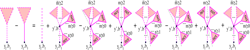
The above-described procedure can be easily generalized to include simple loop contributions, replacing single Pomerons connecting neighboring “cells” of Pomeron “nets” by $t$-channel sequences of Pomerons and Pomeron loops. To this end, one can modify the definition (10) of the “net fan” contributions $\chi_{a(j)|d(l)}^{{\rm net}}$, as shown in Fig. 22,

Figure 22: Generalized “net fan” contribution generates Pomeron nets, whose neighboring “cells” are connected by $t$-channel sequences of Pomerons and Pomeron loops.

i.e.

$$\chi_{a(j)|d(l)}^{{\rm net}}(y_{1},\vec{b}_{1}|Y,\vec{b})=\lambda_{a(j)}\,\chi_{a\mathbb{P}}^{\rm loop}(y_{1},b_{1})+G\int_{0}^{y_{1}}\!dy_{2}\int\!d^{2}b_{2}\;\chi_{\mathbb{PP}}^{\rm loop}(y_{1}-y_{2},|\vec{b}_{1}-\vec{b}_{2}|)$$

$$\times\left\{(1-e^{-\chi_{a(j)|d(l)}^{{\rm net}}\!(y_{2},\vec{b}_{2}|Y,\vec{b})})\;e^{-\chi_{d(l)|a(j)}^{{\rm net}}\!(Y-y_{2},\vec{b}-\vec{b}_{2}|Y,\vec{b})}-\chi_{a(j)|d(l)}^{{\rm net}}(y_{2},\vec{b}_{2}|Y,\vec{b})\right\}\!,$$ (32)

where the contributions $\chi_{a\mathbb{P}}^{\rm loop}$ and $\chi_{\mathbb{PP}}^{\rm loop}$ of Pomeron loop sequences, exchanged between hadron $a$ and the vertex $(y_{1},b_{1})$, respectively, between the vertices $(y_{1},b_{1})$ and $(y_{2},b_{2})$, are defined via the recursive representations of Figs. 23 and 24:

Figure 23: Recursive representation for the contributions of Pomeron loop sequences $\chi_{a\mathbb{P}}^{\rm loop}$, $\chi_{a\mathbb{P}}^{\rm loop(1)}$, exchanged between hadron $a$ and the vertex $(y_{1},b_{1})$.

Figure 24: Recursive representation for the contributions of Pomeron loop sequences $\chi_{\mathbb{PP}}^{\rm loop}$, $\chi_{\mathbb{PP}}^{\rm loop(1)}$, exchanged between the vertices $(y_{1},b_{1})$ and $(y_{2},b_{2})$.

$$\chi_{a\mathbb{P}}^{\rm loop}(y_{1},b_{1})=\chi_{a\mathbb{P}}^{\mathbb{P}}(y_{1},b_{1})$$

$$+G\int_{0}^{y_{1}}\!dy^{\prime}\int\!d^{2}b^{\prime}\,\left[(1-e^{-\chi_{\mathbb{PP}}^{\mathbb{P}}(y_{1}-y^{\prime},|\vec{b}_{1}-\vec{b}^{\prime}|)})\;\chi_{a\mathbb{P}}^{\rm loop}(y^{\prime},b^{\prime})-\chi_{\mathbb{PP}}^{\mathbb{P}}(y_{1}-y^{\prime},|\vec{b}_{1}-\vec{b}^{\prime}|)\;\chi_{a\mathbb{P}}^{\rm loop(1)}(y^{\prime},b^{\prime})\right]$$ (33)

$$\chi_{a\mathbb{P}}^{\rm loop(1)}(y_{1},b_{1})=\chi_{a\mathbb{P}}^{\mathbb{P}}(y_{1},b_{1})+G\int_{0}^{y_{1}}\!dy^{\prime}\int\!d^{2}b^{\prime}\;\chi_{\mathbb{PP}}^{\mathbb{P}}(y_{1}-y^{\prime},|\vec{b}_{1}-\vec{b}^{\prime}|)\left[\chi_{a\mathbb{P}}^{\rm loop}(y^{\prime},b^{\prime})-\chi_{a\mathbb{P}}^{\rm loop(1)}(y^{\prime},b^{\prime})\right]$$ (34)

$$\chi_{\mathbb{PP}}^{\rm loop}(y_{2}-y_{1},|\vec{b}_{2}-\vec{b}_{1}|)=1-e^{-\chi_{\mathbb{PP}}^{\mathbb{P}}(y_{2}-y_{1},|\vec{b}_{2}-\vec{b}_{1}|)}+G\int_{y_{1}}^{y_{2}}\!dy^{\prime}\int\!d^{2}b^{\prime}\,\left[(1-e^{-\chi_{\mathbb{PP}}^{\mathbb{P}}(y^{\prime}-y_{1},|\vec{b}^{\prime}-\vec{b}_{1}|)})\right.$$

$$\times\left.\chi_{\mathbb{PP}}^{\rm loop}(y_{2}-y^{\prime},|\vec{b}_{2}-\vec{b}^{\prime}|)-\chi_{\mathbb{PP}}^{\mathbb{P}}(y^{\prime}-y_{1},|\vec{b}^{\prime}-\vec{b}_{1}|)\;\chi_{\mathbb{PP}}^{\rm loop(1)}(y_{2}-y^{\prime},|\vec{b}_{2}-\vec{b}^{\prime}|)\right]$$ (35)

$$\chi_{\mathbb{PP}}^{\rm loop(1)}(y_{2}-y_{1},|\vec{b}_{2}-\vec{b}_{1}|)=\chi_{\mathbb{PP}}^{\mathbb{P}}(y_{2}-y_{1},|\vec{b}_{2}-\vec{b}_{1}|)$$

$$+G\int_{y_{1}}^{y_{2}}\!dy^{\prime}\int\!d^{2}b^{\prime}\;\chi_{\mathbb{PP}}^{\mathbb{P}}(y^{\prime}-y_{1},|\vec{b}^{\prime}-\vec{b}_{1}|)\;\left[\chi_{\mathbb{PP}}^{\rm loop}(y_{2}-y^{\prime},|\vec{b}_{2}-\vec{b}^{\prime}|)-\chi_{\mathbb{PP}}^{\rm loop(1)}(y_{2}-y^{\prime},|\vec{b}_{2}-\vec{b}^{\prime}|)\right]\!.$$ (36)

Here $\chi_{a\mathbb{P}}^{\rm loop(1)}$ and $\chi_{\mathbb{PP}}^{\rm loop(1)}$ are the contributions of such Pomeron loop sequences (exchanged between hadron $a$ and the vertex $(y_{1},b_{1})$, respectively, between the vertices $(y_{1},b_{1})$ and $(y_{2},b_{2})$), which start from a single Pomeron connected to the vertex $(y_{1},b_{1})$, as shown in Figs. 23, 24.

Redefining in a similar way the fan diagram equation (11), one can literally repeat the analysis of Ref. [14] and obtain the contribution of arbitrary Pomeron nets, with neighboring “cells” being connected by $t$-channel loop sequences, in the form of Eq. (9), with the eikonal $\chi_{\mathbb{PP}}^{\mathbb{P}}(y_{1}-y_{2},|\vec{b}_{1}-\vec{b}_{2}|)$ being replaced by the corresponding loop sequence contribution $\chi_{\mathbb{PP}}^{\rm loop}(y_{1}-y_{2},|\vec{b}_{1}-\vec{b}_{2}|)$, as depicted in Fig. 25 (a), (b).

Figure 25: Irreducible contributions of arbitrary Pomeron nets to elastic scattering amplitude; neighboring net cells are connected by $t$-channel sequences of Pomerons and Pomeron loops.

In addition, one has to consider an exchange of a single $t$-channel loop sequence between hadrons $a$ and $d$, as shown in Fig. 25 (c), (d), such that each of the two hadrons is coupled to a single Pomeron only. The complete eikonal contribution for the considered class of enhanced diagrams is therefore

$$\chi_{ad(jl)}^{{\rm enh}}(Y,b)=G\int_{0}^{Y}\!dy_{1}\int\!d^{2}b_{1}\left\{(1-e^{-\chi_{a|d}^{{\rm net}}(1)})\,(1-e^{-\chi_{d|a}^{{\rm net}}(1)})-\chi_{a|d}^{{\rm net}}(1)\;\chi_{d|a}^{{\rm net}}(1)\right.$$

$$+\lambda_{a(j)}\,\lambda_{d(l)}\,\chi_{d\mathbb{P}}^{\mathbb{P}}(y_{1},b_{1})\left[\chi_{a\mathbb{P}}^{\rm loop}(Y-y_{1},|\vec{b}-\vec{b}_{1}|)-\chi_{a\mathbb{P}}^{\rm loop(1)}(Y-y_{1},|\vec{b}-\vec{b}_{1}|)\right]$$

$$-G\int_{0}^{y_{1}}\!dy_{2}\int\!d^{2}b_{2}\;\chi_{\mathbb{PP}}^{\rm loop}(y_{1}-y_{2},|\vec{b}_{1}-\vec{b}_{2}|)\;\left[(1-e^{-\chi_{a|d}^{{\rm net}}(1)})\,e^{-\chi_{d|a}^{{\rm net}}(1)}-\chi_{a|d}^{{\rm net}}(1)\right]$$

$$\left.\times\left[(1-e^{-\chi_{d|a}^{{\rm net}}(2)})\,e^{-\chi_{a|d}^{{\rm net}}(2)}-\chi_{d|a}^{{\rm net}}(2)\right]\right\}\!,$$ (37)

where we use the same abbreviations as in (9).

The analysis of unitarity cuts of the generalized scheme proceeds similarly to the one described in Sections 3 and 4. For the contribution of fan-like cuts $2\bar{\chi}_{a(j)|d(l)}^{{\rm fan}}-2\tilde{\chi}_{a(j)|d(l)}^{{\rm fan}}$, $2\tilde{\chi}_{a(j)|d(l)}^{{\rm fan}}$ of “net fan” graphs of Fig. 22 one obtains the representations of Fig. 26

Figure 26: Recursive equations for the contributions $2\bar{\chi}_{a(j)|d(l)}^{{\rm fan}}-2\tilde{\chi}_{a(j)|d(l)}^{{\rm fan}}$, $2\tilde{\chi}_{a(j)|d(l)}^{{\rm fan}}$ of fan-like cuts of generalized “net fan” graphs of Fig. 22.

(c.f. Figs. 8, 9), i.e.

$$2\bar{\chi}_{a(j)|d(l)}^{{\rm fan}}(y_{1},\vec{b}_{1}|Y,\vec{b})-2\tilde{\chi}_{a(j)|d(l)}^{{\rm fan}}(y_{1},\vec{b}_{1}|Y,\vec{b})=2\lambda_{a(j)}\,\bar{\chi}_{a\mathbb{P}}^{\rm loop}(y_{1},b_{1})$$

$$+G\int_{0}^{y_{1}}\!dy_{2}\int\!d^{2}b_{2}\;\bar{\chi}_{\mathbb{PP}}^{\rm loop}\left\{\left[(e^{2\bar{\chi}_{a|d}^{{\rm fan}}}-1)\>e^{-2\chi_{a|d}^{{\rm net}}-2\chi_{d|a}^{{\rm net}}}-2\bar{\chi}_{a|d}^{{\rm fan}}\right]\right.$$

$$\left.-2\left[(e^{\tilde{\chi}_{a|d}^{{\rm fan}}}-1)\>e^{-\chi_{a|d}^{{\rm net}}-2\chi_{d|a}^{{\rm net}}}-\tilde{\chi}_{a|d}^{{\rm fan}}\right]+(1-e^{-\chi_{a|d}^{{\rm net}}})^{2}\>e^{-2\chi_{d|a}^{{\rm net}}}\right\}$$ (38)

$$2\tilde{\chi}_{a(j)|d(l)}^{{\rm fan}}(y_{1},\vec{b}_{1}|Y,\vec{b})=G\int_{0}^{y_{1}}\!dy_{2}\int\!d^{2}b_{2}\;\chi_{\mathbb{PP}}^{\rm loop}\left\{(1-e^{-\chi_{d|a}^{{\rm net}}})\>e^{-\chi_{d|a}^{{\rm net}}}\left[(e^{2\bar{\chi}_{a|d}^{{\rm fan}}}-1)\>e^{-2\chi_{a|d}^{{\rm net}}}\right.\right.$$

$$\left.\left.-2\,(e^{\tilde{\chi}_{a|d}^{{\rm fan}}}-1)\>e^{-\chi_{a|d}^{{\rm net}}}+(1-e^{-\chi_{a|d}^{{\rm net}}})^{2}\right]+2\left[(e^{\tilde{\chi}_{a|d}^{{\rm fan}}}-1)\>e^{-\chi_{a|d}^{{\rm net}}-\chi_{d|a}^{{\rm net}}}-\tilde{\chi}_{a|d}^{{\rm fan}}\right]\right\}\!,$$ (39)

where the contributions of cut loop sequences $\bar{\chi}_{a\mathbb{P}}^{\rm loop}$, $\bar{\chi}_{a\mathbb{P}}^{\rm loop(1)}$, $\bar{\chi}_{\mathbb{PP}}^{\rm loop}$, $\bar{\chi}_{\mathbb{PP}}^{\rm loop(1)}$ satisfy the recursive equations of Figs. 27 and 28

Figure 27: Recursive representation for the AGK cuts of Pomeron loop sequences, $\bar{\chi}_{a\mathbb{P}}^{\rm loop}$, $\bar{\chi}_{a\mathbb{P}}^{\rm loop(1)}$, exchanged between hadron $a$ and the vertex $(y_{1},b_{1})$.

Figure 28: Recursive representation for the AGK cuts of Pomeron loop sequences, $\bar{\chi}_{\mathbb{PP}}^{\rm loop}$, $\bar{\chi}_{\mathbb{PP}}^{\rm loop(1)}$, exchanged between the vertices $(y_{1},b_{1})$ and $(y_{2},b_{2})$.

respectively. Clearly, one has

$$\bar{\chi}_{a\mathbb{P}}^{\rm loop}(y_{1},b_{1})=\chi_{a\mathbb{P}}^{\rm loop}(y_{1},b_{1})$$ (40)

$$\bar{\chi}_{a\mathbb{P}}^{\rm loop(1)}(y_{1},b_{1})=\chi_{a\mathbb{P}}^{\rm loop(1)}(y_{1},b_{1})$$ (41)

$$\bar{\chi}_{\mathbb{PP}}^{\rm loop}(y_{1}-y_{2},|\vec{b}_{1}-\vec{b}_{2}|)=\chi_{\mathbb{PP}}^{\rm loop}(y_{1}-y_{2},|\vec{b}_{1}-\vec{b}_{2}|)$$ (42)

$$\bar{\chi}_{\mathbb{PP}}^{\rm loop(1)}(y_{1}-y_{2},|\vec{b}_{1}-\vec{b}_{2}|)=\chi_{\mathbb{PP}}^{\rm loop(1)}(y_{1}-y_{2},|\vec{b}_{1}-\vec{b}_{2}|)\,.$$ (43)

Thus, repeating literally the reasoning of Sections 3 and 4, for the complete set of tree-like AGK cuts of the graphs of Fig. 25 (a), (b) we can obtain the representation of Figs. 16, 17, and 19, with the uncut and fan-like cut “net fans” being defined now as in Figs. 22 and 26 respectively, with the single cut Pomeron contribution $\chi_{d\mathbb{P}}^{\mathbb{P}}$ in Fig. 19 (i), (j) being replaced by the one of the cut loop sequence $\bar{\chi}_{d\mathbb{P}}^{\rm loop}$, and with the t-channel sequences of cut and uncut Pomerons $\chi_{a(j)|d(l)}^{\mathbb{P}_{{\rm cc}}}$ and $\chi_{a(j)|d(l)}^{\mathbb{P}_{{\rm uc}}}$ (depicted as broken Pomeron lines in Fig. 19) being replaced by the ones of loops $\chi_{a(j)|d(l)}^{\rm{loop}_{{\rm cc}}}$, $\chi_{a(j)|d(l)}^{\rm{loop}_{{\rm uc}}}$. For the latter one obtains, similarly to (24-25),

$$2\chi_{a(j)|d(l)}^{\rm{loop}_{{\rm cc}}}(y_{1},\vec{b}_{1}|Y,\vec{b})=2\lambda_{a(j)}\,\chi_{a\mathbb{P}}^{\rm{loop}}(y_{1},b_{1})+2G\int_{0}^{y_{1}}\!dy_{2}\int\!d^{2}b_{2}\;\chi_{\mathbb{PP}}^{\rm{loop}}$$

$$\times\left[(e^{-2\chi_{a|d}^{{\rm net}}-2\chi_{d|a}^{{\rm net}}}-1)\,(\chi_{a|d}^{\rm{loop}_{{\rm cc}}}+\chi_{a|d}^{\rm{loop}_{{\rm uc}}})-(e^{-\chi_{a|d}^{{\rm net}}-2\chi_{d|a}^{{\rm net}}}-1)\,\chi_{a|d}^{\rm{loop}_{{\rm uc}}}\right]$$ (44)

$$2\chi_{a(j)|d(l)}^{\rm{loop}_{{\rm uc}}}(y_{1},\vec{b}_{1}|Y,\vec{b})=2G\int_{0}^{y_{1}}\!dy_{2}\int\!d^{2}b_{2}\;\chi_{\mathbb{PP}}^{\rm{loop}}$$

$$\times\left[(1-e^{-\chi_{d|a}^{{\rm net}}})\,e^{-2\chi_{a|d}^{{\rm net}}-\chi_{d|a}^{{\rm net}}}\,(\chi_{a|d}^{\rm{loop}_{{\rm cc}}}+\chi_{a|d}^{\rm{loop}_{{\rm uc}}})+(e^{-\chi_{a|d}^{{\rm net}}-2\chi_{d|a}^{{\rm net}}}-1)\,\chi_{a|d}^{\rm{loop}_{{\rm uc}}}\right]\!.$$ (45)

In a similar way one generalizes the definition of the $k$-th order cut “net fan” contributions $2\bar{\chi}_{a|d}^{{\rm net}(k)}$ and obtains the representation of Fig. 20 for the complete set of zigzag-like cuts of the diagrams of Fig. 25 (a), (b). Finally, for the graphs of Fig. 25 (c), (d) the cutting procedure is trivial, yielding a convolution of the cut loop sequences $\bar{\chi}_{a\mathbb{P}}^{\rm loop}$ and $\bar{\chi}_{a\mathbb{P}}^{\rm loop(1)}$ of Fig. 27 with the cut Pomeron eikonal $\chi_{d\mathbb{P}}^{\mathbb{P}}$:

$$2G\int_{0}^{Y}\!dy_{1}\int\!d^{2}b_{1}\;\lambda_{a(j)}\,\lambda_{d(l)}\,\chi_{d\mathbb{P}}^{\mathbb{P}}(y_{1},b_{1})\left[\bar{\chi}_{a\mathbb{P}}^{\rm loop}(Y-y_{1},|\vec{b}-\vec{b}_{1}|)-\bar{\chi}_{a\mathbb{P}}^{\rm loop(1)}(Y-y_{1},|\vec{b}-\vec{b}_{1}|)\right]\!.$$ (46)

The described generalization of the scheme appears to be sufficient to cure the above-mentioned problems with the violation of the $s$-channel unitarity in certain kinematic regions. In the considered case of double high mass diffraction, in addition to the graph of Fig. 21 (left) one obtains now the loop diagram of Fig. 21 (right), such that the summary contribution becomes

$$\sigma_{ad}^{\rm DD}(s,y_{1},y_{2})\simeq\frac{G}{4}\sum_{j,l}C_{a(j)}\,C_{d(l)}\int\!d^{2}b\,d^{2}b_{1}\,d^{2}b_{1}\;(1-e^{-2\lambda_{a(j)}\,\chi_{a\mathbb{P}}^{\mathbb{P}}(Y-y_{2},|\vec{b}-\vec{b}_{2}|)})$$

$$\times(1-e^{-2\lambda_{d(l)}\,\chi_{d\mathbb{P}}^{\mathbb{P}}(y_{1},b_{1})})\;(1-e^{-\chi_{\mathbb{PP}}^{\mathbb{P}}(y_{2}-y_{1},|\vec{b}_{2}-\vec{b}_{1}|)})\;e^{-\lambda_{a(j)}\,\chi_{a\mathbb{P}}^{\mathbb{P}}(Y-y_{1},|\vec{b}-\vec{b}_{1}|)}\;e^{-\lambda_{d(l)}\,\chi_{d\mathbb{P}}^{\mathbb{P}}(y_{2},b_{2})}$$

$$\times\left[(1-e^{-\chi_{\mathbb{PP}}^{\mathbb{P}}(y_{2}-y_{1},|\vec{b}_{2}-\vec{b}_{1}|)})\;e^{-\lambda_{a(j)}\,\chi_{a\mathbb{P}}^{\mathbb{P}}(Y-y_{1},|\vec{b}-\vec{b}_{1}|)}\;e^{-\lambda_{d(l)}\,\chi_{d\mathbb{P}}^{\mathbb{P}}(y_{2},b_{2})}\right.$$

$$-\left.2\,(1-e^{-\lambda_{a(j)}\,\chi_{a\mathbb{P}}^{\mathbb{P}}(Y-y_{1},|\vec{b}-\vec{b}_{1}|)})\;(1-e^{-\lambda_{d(l)}\,\chi_{d\mathbb{P}}^{\mathbb{P}}(y_{2},b_{2})})\right]S^{\rm RG}_{ad(jl)}(Y,b,y_{1},y_{2})\,.$$ (47)

In the region of large impact parameters, which gives the dominant contribution to (47), either $\chi_{a\mathbb{P}}^{\mathbb{P}}(Y-y_{1},|\vec{b}-\vec{b}_{1}|)$ or/and $\chi_{d\mathbb{P}}^{\mathbb{P}}(y_{2},b_{2})$ is small. Thus, the expression in the square brackets reduces to

$$\chi_{\mathbb{PP}}^{\mathbb{P}}(y_{2}-y_{1},|\vec{b}_{2}-\vec{b}_{1}|)-2\,\lambda_{a(j)}\,\lambda_{d(l)}\,\chi_{a\mathbb{P}}^{\mathbb{P}}(Y-y_{1},|\vec{b}-\vec{b}_{1}|)\,\chi_{d\mathbb{P}}^{\mathbb{P}}(y_{2},b_{2})>0$$

and assures a positive result for $\sigma_{ad}^{\rm DD}$. A systematic analysis of hadronic final states, obtained in the described scheme, will be presented elsewhere [16].

6 Conclusions

We proposed here a method for a re-summation of the full set of AGK-based unitarity cuts of a very general class of net-like enhanced Pomeron diagrams. This is the principal novelty of the present analysis compared to other related works [6, 7, 8], which have been restricted to investigations of contributions of particular, notably diffractive, final states only. Though the main derivation has been performed for the class of non-loop net-like diagrams, we have demonstrated that the method can be trivially generalized to include Pomeron loop contributions. In the latter case, one simply considers neighboring cells of Pomeron nets to be connected by (cut or uncut) $t$-channel sequences of Pomerons and Pomeron loops, rather than by single Pomeron exchanges; the same applies for the connections between initial hadrons and the correspondingly neighboring net cells. In a similar way one can include more general loop contributions [16].

Although the obtained expressions for the contributions of cut enhanced diagrams are based on a particular eikonal ansatz (8) for multi-Pomeron vertices, the corresponding diagrammatic representations, e.g. of Figs. 4, 5, 8, 9, 16, 17, 19, 20, are of more general character and remain applicable for arbitrary parameterizations of multi-Pomeron vertices.

It is noteworthy that current analysis does not depend on a particular parameterization for the Pomeron exchange amplitude and can be extended for a phenomenological description of “hard” partonic processes [15]. In principle, the proposed method can be also applied in the perturbative BFKL Pomeron framework. However, one should keep in mind that the principal assumption of the present analysis was that the AGK cutting rules remain valid, in particular, that multi-Pomeron vertices remain unmodified by the cutting procedure. The fact that the AGK rules are not proven in QCD, with some deviations from the AGK prescriptions already reported in literature [17], implies that the method may have to be significantly modified, when employed in the BFKL Pomeron calculus. On the other hand, recent investigations indicate that the AGK picture still remains a reasonably good approximation in the pQCD framework [18].

The obtained results open the way for a consistent implementation of the RFT in hadronic MC models. Details of the corresponding procedure will be discussed elsewhere [16]. On the other hand, the scheme can be applied for calculations of total and diffractive hadronic cross sections and of rapidity gap survival probabilities, a preliminary analysis already reported in [15].

References

[1]
V. N. Gribov, Sov. Phys. JETP 26, 414 (1968);
ibid.29, 483 (1969);
M. Baker and K. A. Ter-Martirosian, Phys. Rep. 28, 1 (1976).
[2] L. V. Gribov, E. M. Levin and M. G. Ryskin,
Phys. Rep. 100, 1 (1983).
[3]
A. B. Kaidalov, Phys. Rep. 50, 157 (1979);
A. B. Kaidalov and K. A. Ter-Martirosyan,
Phys. Lett. B 117, 247 (1982);
A. Capella et al., Phys. Rep. 236, 225 (1994).
[4] E. Gotsman, E. M. Levin and U. Maor,
Phys. Lett. B 309, 199 (1993); Phys. Rev. D 49, 4321 (1994);
Phys. Lett. B 452, 387 (1999); Phys. Rev. D 60, 094011 (1999);
S. Bondarenko and E. Levin,
Eur. Phys. J. C 51, 659 (2007);
E. Gotsman, A. Kormilitzin, E. Levin and U. Maor,
Eur. Phys. J. C 52, 295 (2007).
[5] V. A. Khoze, A. D. Martin and M. G. Ryskin,
Eur. Phys. J. C 18, 167 (2000);
Nucl. Phys. Proc. Suppl. 99B, 213 (2001);
A. B. Kaidalov, V. A. Khoze, A. D. Martin and M. G. Ryskin,
Eur. Phys. J. C 21, 521 (2001);
Acta Phys. Polon. B 34, 3163 (2003).
[6] S. Bondarenko, E. Gotsman, E. Levin and U. Maor,
Nucl. Phys. A 683, 649 (2001).
[7] K. G. Boreskov, A. B. Kaidalov, V. A. Khoze,
A. D. Martin and M. G. Ryskin,
Eur. Phys. J. C 44, 523 (2005).
[8] M. G. Ryskin, A. D. Martin and V. A. Khoze,
arXiv:0710.2494 [hep-ph].
[9]
P. Aurenche et al., Phys. Rev. D 45, 92 (1992);
K. Werner, Phys. Rep. 232, 87 (1993);
N. N. Kalmykov and S. S. Ostapchenko,
Phys. At. Nucl. 56, 346 (1993);
N. N. Kalmykov, S. S. Ostapchenko and A. I. Pavlov,
Nucl. Phys. Proc. Suppl. 52B, 17 (1997);
H. J. Drescher, M. Hladik, S. Ostapchenko, T. Pierog and K. Werner,
Phys. Rep. 350, 93 (2001).
[10]
M. Braun, Sov. J. Nucl. Phys. 52, 164 (1990);
V. A. Abramovskii and G. G. Leptoukh, ibid.55, 903 (1992);
M. Hladik, H. J. Drescher, S. Ostapchenko, T. Pierog and K. Werner,
Phys. Rev. Lett. 86, 3506 (2001).
[11]
V. A. Abramovskii, V. N. Gribov and O. V. Kancheli,
Sov. J. Nucl. Phys. 18, 308 (1974).
[12] O. V. Kancheli, JETP Lett. 18, 274 (1973);
A. Schwimmer, Nucl. Phys. B 94, 445 (1975);
A. Capella, J. Kaplan and J. Tran Thanh Van, ibid.105, 333
(1976);
V. A. Abramovskii, JETP Lett. 23, 228 (1976);
M. S. Dubovikov and K. A. Ter-Martirosyan, Nucl. Phys. B 124, 163
(1977);
[13]
J. L. Cardi, Nucl. Phys. B 75, 413 (1974);
A. B. Kaidalov, L. A. Ponomarev and K. A. Ter-Martirosyan,
Sov. J. Nucl. Phys. 44 (1986) 468.
[14]
S. Ostapchenko, Phys. Lett. B 636, 40 (2006).
[15]
S. Ostapchenko, Phys. Rev. D 74, 014026 (2006).
[16]
S. Ostapchenko, in preparation.
[17] N. N. Nikolaev and W. Schafer, Phys. Rev. D 74, 074021 (2006).
[18] J. Bartels, M. Salvadore and G. P. Vacca, Eur. Phys. J. C 42, 53 (2005);
M. Salvadore, J. Bartels and G. P. Vacca, arXiv:0709.3062 [hep-ph].