Tevatron-for-LHC Report: Higgs

Abstract

The search for Higgs bosons in both the standard model and its extensions is well under way at the Tevatron. As the integrated luminosity collected increases into the multiple inverse femptobarn range, these searches are becoming very interesting indeed. Meanwhile, the construction of the Large Hadron Collider (LHC) and its associated experiments at CERN are nearing completion. In this TeV4LHC workshop, it was realized that any experience at the Tevatron with respect to backgrounds, experimental techniques and theoretical calculations that can be verified at the Tevatron which have relevance for future measurements at the LHC were important. Studies and contributions to these efforts were made in three broad categories: theoretical calculations of Higgs production and decay mechanisms; theoretical calculations and discussions pertaining to non-standard model Higgs bosons; and experimental reviews, analyses and developments at both the Tevatron and the upcoming LHC experiments. All of these contributions represent real progress towards the elucidation of the mechanism of electroweak symmetry breaking.

^¶ Convenors of the Higgs Working Group
^† Organizers of the TeV4LHC Workshop

1 Introduction

Contributed by: S. Willenbrock, A. Dominguez, I. Iashvilli

The Fermilab Tevatron, which has been colliding protons and antiprotons for over twenty years, was not designed to search for the Higgs boson. However, the advent of high-efficiency $b$ tagging, developed in the context of the search for the top quark, made it possible to consider searching for the Higgs boson, produced in association with a weak boson, via the decay $h\to b\bar{b}$ [1]. It was realized that this would require very high luminosity, and that other discovery modes, such as $h\to W^{+}W^{-}\to\ell^{+}\ell^{-}\nu\bar{\nu}$, might also become viable with sufficient integrated luminosity [2]. The strategy for the Standard Model Higgs search was developed in the TeV2000 workshop [3], and was further refined, along with the case of the supersymmetric Higgs, in the SUSY/Higgs workshop [4].

The search for a Higgs boson, both standard and supersymmetric, is in full swing at the Tevatron, and is becoming increasingly interesting as the integrated luminosity mounts. Meanwhile, the construction of the CERN Large Hadron Collider (LHC) is nearing completion. At this workshop, dubbed TeV4LHC, the Higgs working group used the first meeting to decide what “TeV4LHC” means in the context of the Higgs boson. We decided that anything having to do with the Higgs at the Tevatron was relevant to the workshop, since this experience will surely be valuable at the LHC. Any experience at the Tevatron with backgrounds to Higgs searches is also relevant to the workshop. Finally, any experimental techniques being developed for the Higgs search at the Tevatron or the LHC should also be included in the workshop.

The proceedings of the Higgs working group comprises a large number of contributions on a wide variety of topics. Roughly speaking, the contributions fall into one of three categories.

The first category is theoretical calculations of Higgs production and decay processes, including higher-order corrections and resummation to all orders. There is an overview of Higgs total cross sections, both in the Standard Model and with supersymmetry. There is a review of calculations of Higgs production in association with heavy quarks, either bottom or top. In the case of Higgs production in association with bottom quarks, there is a discussion of the Higgs transverse momentum distribution, including the resummation of soft gluons, for both inclusive Higgs production as well as production in association with a high-$P_{T}$ $b$ jet. These calculations make use of the $b$ distribution function in the proton, and there is a contribution regarding sets of parton distribution functions with no heavy quarks, with only $c$ quarks, or with both $c$ and $b$ quarks, at next-to-next-to-leading order in QCD. Finally, there is a calculation of the electroweak corrections to Higgs production via $gg\to h$, which is the dominant production mechanism.

The second category is non-standard Higgs bosons, either with or without supersymmetry. There is a discussion of the impact of radiative corrections on the search for supersymmetric Higgs bosons at the Tevatron and the LHC. There is an analysis of the search for a Higgs decaying via $h\to aa\to b\bar{b}\tau^{+}\tau^{-}$ at the Tevatron, where $a$ is also a Higgs scalar (or pseudoscalar). There is a discussion on how to use the processes $b\bar{b}\to h$, $h\to\tau^{+}\tau^{-}$, and $h\to\gamma\gamma$ to disentangle the nature of electroweak symmetry breaking. Methods to search for a Higgs boson that decays invisibly are proposed. Finally, there is a discussion of the search for charged Higgs bosons at hadron colliders.

The third category is experimental reviews, analyses, and developments. There are reviews from both CDF and D0 on the status and prospects for Higgs searches at the Tevatron. There are studies on $b$ jets, one on $Z\to b\bar{b}$ and the other on improving the $b$-jet resolution. There are studies on $h\to W^{+}W^{-}\to\ell^{+}\ell^{-}\nu\bar{\nu}$ and $h\to\tau^{+}\tau^{-}$ at the LHC. There is a discussion of the diphoton background at the Tevatron, which is relevant to the search for the Higgs via $h\to\gamma\gamma$ at the LHC.

All of these contributions represent real progress towards the elucidation of the mechanism of electroweak symmetry breaking. It will require the best efforts of us all to extract the maximal information from the data coming from the Tevatron and the LHC.

Acknowledgment

This material is based upon work supported by the National Science Foundation under Grant Number 0547780.

2 SM and MSSM Higgs Boson Production Cross Sections

Contributed by: T. Hahn, S. Heinemeyer, F. Maltoni, S. Willenbrock

We present the SM and MSSM Higgs-boson production cross sections at the Tevatron and the LHC. The SM cross sections are a compilation of state-of-the-art theoretical predictions. The MSSM cross sections are obtained from the SM ones by means of an effective coupling approximation, as implemented in FeynHiggs. Numerical results have been obtained in four benchmark scenarios for two values of $\tan\beta$, $\tan\beta=5,40$.

2.1 Introduction

Deciphering the mechanism of electroweak symmetry breaking (EWSB) is one of the main quests of the high energy physics community. Electroweak precision data in combination with the direct top-quark mass measurement at the Tevatron have strongly constrained the range of possible scenarios and hinted to the existence of a light scalar particle [5]. Both in the standard model (SM) and in its minimal supersymmetric extensions (MSSM), the $W$ and $Z$ bosons and fermions acquire masses by coupling to the vacuum expectation value(s) of scalar SU(2) doublet(s), via the so-called Higgs mechanism. The common prediction of such models is the existence of at least one scalar state, the Higgs boson. Within the SM, LEP has put a lower bound on the Higgs mass, $m_{h}>114$ GeV [6], and has contributed to the indirect evidence that the Higgs boson should be relatively light with a 95% probability for its mass to be below 186 GeV [5]. In the MSSM the experimental lower bound for the mass of the lightest state is somewhat weaker, and internal consistency of the theory predicts an upper bound of 135 GeV [7, 8, 9].

If the Higgs sector is realized as implemented in the SM or the MSSM, at least one Higgs boson should be discovered at the Tevatron and/or at the LHC. Depending on the mass, there are various channels available where Higgs searches can be performed. The power of each signature depends on the production cross section, $\sigma$, and the Higgs branching ratio into final state particles, such as leptons or $b$-jets, the total yield of events being proportional to $\sigma\cdot$ BR. In some golden channels, such as $gg\to h\to Z^{(*)}Z\to 4\mu$, a discovery will be straightfoward and mostly independent from our ability to predict signal and/or backgrounds. On the other hand, for coupling measurements or for searches in more difficult channels, such as $t\bar{t}h\to t\bar{t}b\bar{b}$ associated production, precise predictions for both signal and backgrounds are mandatory. Within the MSSM such precise predictions for signal and backgrounds are necessary in order to relate the experimental results to the underlying SUSY parameters.

The aim of this note is to collect up-to-date predictions for the most relevant signal cross sections, for both the SM and the MSSM. In Section 2.2 we collect the results of state-of-the-art calculations for the SM cross sections as a function of the Higgs mass. In Section 2.3 we present the MSSM cross sections for the neutral Higgs-bosons in four benchmark scenarios. These results are obtained by rescaling the SM cross sections presented in the previous sections, using an effective coupling approximation.

2.2 SM Higgs production cross sections

In this section we collect the predictions for the most important SM Higgs production processes at the Tevatron and at the LHC. The relevant cross sections are presented in Figs. 2.2.1 and 2.2.2 as function of the Higgs mass. The results refer to fully inclusive cross sections. No acceptance cuts or branching ratios are applied. We do not consider here diffractive Higgs production, $pp\to p\oplus H\oplus p$ [10, 11, 12, 13, 14]. For the discussion of this channel in the MSSM we refer to Ref. [15].

We do not aim here at a detailed discussion of the importance of each signature at the Tevatron or the LHC, but only at providing the most accurate and up-to-date theoretical predictions. To gauge the progress made in the last years, it is interesting to compare the accuracy of the results available in the year 2000, at the time of the Tevatron Higgs Working Group  [4], with those shown here. All relevant cross sections are now known at least one order better in the strong-coupling expansion, and in some cases also electroweak corrections are available.

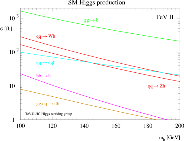
Figure 2.2.1: Higgs-boson production cross sections (fb) at the Tevatron ($\sqrt{s}=1.96$ TeV) for the most relevant production mechanims as a function of the Higgs-boson mass. Results for $gg\to h$, $q\bar{q}\to Vh$, $b\bar{b}\to h$ are at NNLO in the QCD expansion. Weak boson fusion ($qq\to qqh$) and $t\bar{t}$ associated production are at NLO accuracy.

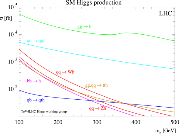
Figure 2.2.2: Higgs-boson production cross sections (fb) at the LHC ($\sqrt{s}=14$ TeV) for the most relevant production mechanims as a function of the Higgs-boson mass. Results for $gg\to h$, $q\bar{q}\to Vh$, $b\bar{b}\to h$ are at NNLO in the QCD expansion. Weak boson fusion ($qq\to qqh$) and $t\bar{t}$ associated production are at NLO accuracy. Single-top associated production ($qb\to qth$) is at LO.

• $gg\to h+X$: gluon fusion
  

  This process is known at NNLO in QCD [16, 17, 18] (in the large top-mass limit) and at NLO in QCD for a quark of an arbitrary mass circulating in the loop [19, 20]. Some N³LO results have recently been obtained in Refs. [21, 22]. The NNLO results plotted here are from Ref. [23] and include soft-gluon resummation effects at NNLL. MRST2002 at NNLO has been used [24], with the renormalization and factorization scales set equal to the Higgs-boson mass. The overall residual theoretical uncertainty is estimated to be around 10%. The uncertainties due to the large top mass limit approximation (beyond Higgs masses of $2\times m_{t}$) are difficult to estimate but expected to be relatively small. Differential results at NNLO are also available [25]. NLO (two-loop) EW corrections are known for Higgs masses below $2m_{W}$, [26, 27], and range between 5% and 8% of the lowest order term. These EW corrections, however, are not included in Figs. 2.2.1, 2.2.2, and they are also omitted in the MSSM evaluations below. The same holds for the recent corrections obtained in Refs. [21, 22].

• $qq\to qqh+X$: vector boson fusion
  

  This process is known at NLO in QCD [28, 29, 30]. Results plotted here have been obtained with MCFM[31]. Leading EW corrections are taken into account by using $\alpha(M_{Z})$ as the (square of the) electromagnetic coupling. The PDF used is CTEQ6M [32] and the renormalization and factorization scales are set equal to the Higgs-boson mass. The theoretical uncertainty is rather small, less than 10%.

• $q\bar{q}\to Vh+X$: $W,Z$ associated production
  

  These processes are known at NNLO in the QCD expansion [33] and at NLO in the electroweak expansion [34]. The results plotted here have been obtained by the LH2003 Higgs working group by combining NNLO QCD and NLO EW corrections [35]. The PDF used is MRST2001 and the renormalization and factorization scales are set equal to the Higgs-vector-boson invariant mass. The residual theoretical uncertainty is rather small, less than 5%.

• $b\bar{b}\to h+X$: bottom fusion
  

  This process is known at NNLO in QCD in the five-flavor scheme [36]. The cross section in the four-flavor scheme is known at NLO [37, 38]. Results obtained in the two schemes have been shown to be consistent [35, 39, 40]. The results plotted here are from Ref. [36]. MRST2002 at NNLO has been used, with the renormalization scale set equal to $m_{h}$ and the factorization scale set equal to $m_{h}/4$. For results with one final-state $b$-quark at high-$p_{T}$ we refer to Ref. [41, 39]. For results with two final-state $b$-quarks at high-$p_{T}$ we refer to Ref. [37, 38].

• $q\bar{q},gg\to t\bar{t}h+X$: $t\bar{t}$ associated production
  

  This process is known at NLO in QCD [42, 43, 44]. The results plotted here are from Ref. [44]. The PDF used is CTEQ6M and the renormalization and factorization scales are set equal to $m_{t}+m_{h}/2$.

• $qb\to qth$ : single-top associated production
  

  This process is known at LO in QCD [45]. The results plotted here ($t$-channel production, LHC only) are from Ref. [46]. The PDF used is CTEQ5L and the renormalization and factorization scales are set equal to the Higgs-boson mass.

2.3 MSSM Higgs production cross sections

The MSSM requires two Higgs doublets, resulting in five physical Higgs boson degrees of freedom. These are the light and heavy $\mathcal{C}P$-even Higgs bosons, $h$ and $H$, the $\mathcal{C}P$-odd Higgs boson, $A$, and the charged Higgs boson, $H^{\pm}$. The Higgs sector of the MSSM can be specified at lowest order in terms of $M_{Z}$, $M_{A}$, and $\tan\beta\equiv v_{2}/v_{1}$, the ratio of the two Higgs vacuum expectation values. The masses of the $\mathcal{C}P$-even neutral Higgs bosons and the charged Higgs boson can be calculated, including higher-order corrections, in terms of the other MSSM parameters.

After the termination of LEP in the year 2000 (the final LEP results can be found in Refs. [6, 47]), the Higgs boson search has shifted to the Tevatron and will later be continued at the LHC. For these analyses and investigations a precise prediction of the Higgs boson masses, branching ratios and production cross sections in the various channels is necessary.

Due to the large number of free parameters, a complete scan of the MSSM parameter space is too involved. Therefore the search results at LEP [47] and the Tevatron [48, 49, 50], as well as studies for the LHC [51] have been performed in several benchmark scenarios [52, 53, 54].

The code FeynHiggs [55, 7, 8] provides a precise calculation of the Higgs boson mass spectrum, couplings and the decay widths. This has now been supplemented by the evaluation of all relevant neutral Higgs boson production cross sections at the Tevatron and the LHC (and the corresponding three SM cross sections for both colliders with $M_{H}^{\rm SM}=m_{h},m_{H},m_{A}$). They are calculated by using the effective coupling approach, rescaling the SM result.

In this section we will briefly describe the benchmark scenarios with their respective features. The effective coupling approach, used to obtain the production cross sections within FeynHiggs, is discussed. Results for the neutral Higgs production cross sections at the Tevatron and the LHC are presented within the benchmark scenarios for two values of $\tan\beta$, $\tan\beta=5,40$.

2.4 The benchmark scenarios

We start by recalling the four benchmark scenarios [53] suitable for the MSSM Higgs boson search at hadron colliders. In these scenarios the values of the parameters of the $\tilde{t}$ and $\tilde{b}$ sector as well as the gaugino masses are fixed, while $\tan\beta$ and $M_{A}$ are the parameters that are varied. Here we fix $\tan\beta$ to a low and a high value, $\tan\beta=5,40$, but vary $M_{A}$. This also yields a variation of $M_{h}$ and $m_{H}$.

In order to fix our notations, we list the conventions for the inputs from the scalar top and scalar bottom sector of the MSSM: the mass matrices in the basis of the current eigenstates $\tilde{t}_{L},\tilde{t}_{R}$ and $\tilde{b}_{L},\tilde{b}_{R}$ are given by

$${\cal M}^{2}_{\tilde{t}} = \left(\begin{array}[]{cc}M_{\tilde{t}_{L}}^{2}+m_{t}^{2}+\cos 2\beta(\frac{1}{2}-\frac{2}{3}s_{\mathrm{w}}^{2})M_{Z}^{2}&m_{t}X_{t}\\ m_{t}X_{t}&M_{\tilde{t}_{R}}^{2}+m_{t}^{2}+\frac{2}{3}\cos 2\beta s_{\mathrm{w}}^{2}M_{Z}^{2}\end{array}\right),$$ (2.4.3)

$${\cal M}^{2}_{\tilde{b}} = \left(\begin{array}[]{cc}M_{\tilde{b}_{L}}^{2}+m_{b}^{2}+\cos 2\beta(-\frac{1}{2}+\frac{1}{3}s_{\mathrm{w}}^{2})M_{Z}^{2}&m_{b}X_{b}\\ m_{b}X_{b}&M_{\tilde{b}_{R}}^{2}+m_{b}^{2}-\frac{1}{3}\cos 2\beta s_{\mathrm{w}}^{2}M_{Z}^{2}\end{array}\right),$$ (2.4.6)

where

$$m_{t}X_{t}=m_{t}(A_{t}-\mu\cot\beta),\quad m_{b}\,X_{b}=m_{b}\,(A_{b}-\mu\tan\beta).$$ (2.4.7)

Here $A_{t}$ denotes the trilinear Higgs–stop coupling, $A_{b}$ denotes the Higgs–sbottom coupling, and $\mu$ is the higgsino mass parameter. SU(2) gauge invariance leads to the relation

$$M_{\tilde{t}_{L}}=M_{\tilde{b}_{L}}.$$ (2.4.8)

For the numerical evaluation, a convenient choice is

$$M_{\tilde{t}_{L}}=M_{\tilde{b}_{L}}=M_{\tilde{t}_{R}}=M_{\tilde{b}_{R}}=:M_{\mathrm{SUSY}}.$$ (2.4.9)

The parameters in the $\tilde{t}/\tilde{b}$ sector are defined here as on-shell parameters, see Ref. [56] for a discussion and a translation to $\overline{\mathrm{DR}}$ parameters. The top-quark mass is taken to be $m_{t}=m_{t}^{\rm exp}=172.7\mathrm{\ Ge\kern-1.00006ptV}$ [57].

• The $m_{h}^{\mathrm{max}}$ scenario:

  This scenario had been designed to obtain conservative $\tan\beta$ exclusion bounds [58]. The parameters are chosen such that the maximum possible Higgs-boson mass as a function of $\tan\beta$ is obtained (for fixed $M_{\mathrm{SUSY}}$ and $m_{t}$, and $M_{A}$ set to its maximal value, $M_{A}=1\mathrm{\ Te\kern-1.00006ptV}$). The parameters are:

  $$M_{\mathrm{SUSY}}=1\mathrm{\ Te\kern-1.00006ptV},\;\mu=200\mathrm{\ Ge\kern-1.00006ptV},\;M_{2}=200\mathrm{\ Ge\kern-1.00006ptV},$$

  $$X_{t}=2\,M_{\mathrm{SUSY}}\;A_{b}=A_{t},m_{\tilde{g}}=0.8\,M_{\mathrm{SUSY}}~{}.$$ (2.4.10)

• The no-mixing scenario:

  This benchmark scenario is associated with vanishing mixing in the $\tilde{t}$ sector and with a higher SUSY mass scale as compared to the $m_{h}^{\mathrm{max}}$ scenario to increase the parameter space that avoids the LEP Higgs bounds:

  $$M_{\mathrm{SUSY}}=2\mathrm{\ Te\kern-1.00006ptV},\;\mu=200\mathrm{\ Ge\kern-1.00006ptV},\;M_{2}=200\mathrm{\ Ge\kern-1.00006ptV},$$

  $$X_{t}=2\,M_{\mathrm{SUSY}}\;A_{b}=A_{t},m_{\tilde{g}}=0.8\,M_{\mathrm{SUSY}}~{}.$$ (2.4.11)

• The gluophobic Higgs scenario:

  In this scenario the main production cross section for the light Higgs boson at the LHC, $gg\to h$, can strongly suppressed for a wide range of the $M_{A}-\tan\beta$-plane. This happens due to a cancellation between the top quark and the stop quark loops in the production vertex (see Ref. [59]). This cancellation is more effective for small $\tilde{t}$ masses and for relatively large values of the $\tilde{t}$ mixing parameter, $X_{t}$. The partial width of the most relevant decay mode, $\Gamma(h\to\gamma\gamma)$, is affected much less, since it is dominated by the $W$ boson loop. The parameters are:

  $$M_{\mathrm{SUSY}}=350\mathrm{\ Ge\kern-1.00006ptV},\;\mu=300\mathrm{\ Ge\kern-1.00006ptV},\;M_{2}=300\mathrm{\ Ge\kern-1.00006ptV},$$

  $$X_{t}=-750\mathrm{\ Ge\kern-1.00006ptV}\;A_{b}=A_{t},m_{\tilde{g}}=500\mathrm{\ Ge\kern-1.00006ptV}~{}.$$ (2.4.12)

• The small $\alpha_{\rm eff}$ scenario:

  Besides the channel $gg\to h\to\gamma\gamma$ at the LHC, the other channels for light Higgs searches at the Tevatron and at the LHC mostly rely on the decays $h\to b\bar{b}$ and $h\to\tau^{+}\tau^{-}$. Including Higgs-propagator corrections the couplings of the lightest Higgs boson to down-type fermions is $\sim\sin\alpha_{\rm eff}$, where $\alpha_{\rm eff}$ is the loop corrected mixing angle in the neutral $\mathcal{C}P$-even Higgs sector. Thus, if $\alpha_{\rm eff}$ is small, the two main decay channels can be heavily suppressed in the MSSM compared to the SM case. Such a suppression occurs for large $\tan\beta$ and not too large $M_{A}$. The parameters of this scenario are:

  $$M_{\mathrm{SUSY}}=800\mathrm{\ Ge\kern-1.00006ptV},\;\mu=2.5\,M_{\mathrm{SUSY}},\;M_{2}=500\mathrm{\ Ge\kern-1.00006ptV},$$

  $$X_{t}=-1100\mathrm{\ Ge\kern-1.00006ptV},\;A_{b}=A_{t},m_{\tilde{g}}=500\mathrm{\ Ge\kern-1.00006ptV}~{}.$$ (2.4.13)

2.5 The effective coupling approximation

We consider the following neutral Higgs production cross sections at the Tevatron and the LHC ($\phi$ denotes all neutral MSSM Higgs bosons, $\phi=h,H,A$):

$$gg \to \phi+X~{},$$ (2.5.14)

$$qq \to qq\phi+X~{},$$ (2.5.15)

$$q\bar{q} \to W/Z\phi+X~{},$$ (2.5.16)

$$b\bar{b} \to \phi+X~{},$$ (2.5.17)

$$gg,qq \to t\bar{t}\phi~{}.$$ (2.5.18)

The MSSM cross sections have been obtained by rescaling the corresponding SM cross sections of Section 2.2 either with ratio of the corresponding MSSM decay with (of the inverse process) over the SM decay width, or with the square of the ratio of the corresponding couplings. More precisely, we apply the following factors:

• $gg\to\phi+X$:

  $$\frac{\Gamma(\phi\to gg)_{\mathrm{MSSM}}}{\Gamma(\phi\to gg)_{\mathrm{SM}}}$$ (2.5.19)

  We include the full one-loop result with SM QCD corrections. MSSM two-loop corrections [60] have been neglected.

• $qq\to qq\phi+X$:

  $$\frac{|g_{\phi VV,\mathrm{MSSM}}|^{2}}{|g_{\phi VV,\mathrm{SM}}|^{2}},\;V=W,Z~{}.$$ (2.5.20)

  We include the full set of Higgs propagator corrections in the effective couplings.

• $qq\to W/Z\phi+X$:

  $$\frac{|g_{\phi VV,\mathrm{MSSM}}|^{2}}{|g_{\phi VV,\mathrm{SM}}|^{2}},\;V=W,Z~{}.$$ (2.5.21)

  We include the full set of Higgs propagator corrections in the effective couplings.

• $b\bar{b}\to\phi+X$:

  $$\frac{\Gamma(\phi\to b\bar{b})_{\mathrm{MSSM}}}{\Gamma(\phi\to b\bar{b})_{\mathrm{SM}}}~{}.$$ (2.5.22)

  We include here one-loop SM QCD and SUSY QCD corrections, as well as the resummation of all terms of ${\cal O}((\alpha_{s}\tan\beta)^{n})$.

• $gg,qq\to t\bar{t}\phi$:

  $$\frac{|g_{\phi t\bar{t},\mathrm{MSSM}}|^{2}}{|g_{\phi t\bar{t},\mathrm{SM}}|^{2}}~{},$$ (2.5.23)

  where $g_{\phi t\bar{t},\mathrm{MSSM}}$ and $g_{\phi t\bar{t},\mathrm{SM}}$ are composed of a left- and a right-handed part. We include the full set of Higgs propagator corrections in the effective couplings.

In the effective couplings introduced in eqs. (2.5.19)–(2.5.23) we have used the proper normalization of the external (on-shell) Higgs bosons as discussed in Ref. [61].

It should be noted that the effective coupling approximation as described above does not take into account the MSSM-specific dynamics of the production processes. The theoretical uncertainty in the predictions for the cross sections will therefore in general be somewhat larger than for the decay widths.

2.6 Results

Results for the neutral Higgs production cross sections at the Tevatron and the LHC are presented within the four benchmark scenarios for two values of $\tan\beta$, $\tan\beta=5,40$, giving a total of eight plots for each collider.

Figs. 2.6.3 and 2.6.4 show the results for the Tevatron, while Figs. 2.6.5 and 2.6.6 show the LHC results. In Fig. 2.6.3 (2.6.5) the Higgs production cross sections for the neutral MSSM Higgs bosons at the Tevatron (LHC) in the $m_{h}^{\rm max}$ scenario (upper row) and the no-mixing scenario (lower row) can be found. Fig. 2.6.4 (2.6.6) depicts the same for the gluophobic Higgs scenario (upper row) and the small $\alpha_{\rm eff}$ scenario (lower row).

For low $M_{A}$ values the production cross section of the $h$ and the $A$ are similar, while for large $M_{A}$ the cross sections of $H$ and $A$ are very close. This effect is even more pronounced for large $\tan\beta$.

The results presented in this paper have been obtained for the MSSM with real parameters, i.e. the $\mathcal{C}P$-conserving case. They can can easily be extended via the effective coupling approximation to the case of non-vanishing complex phases (as implemented in FeynHiggs).

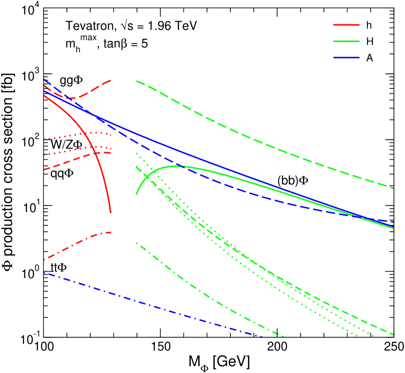
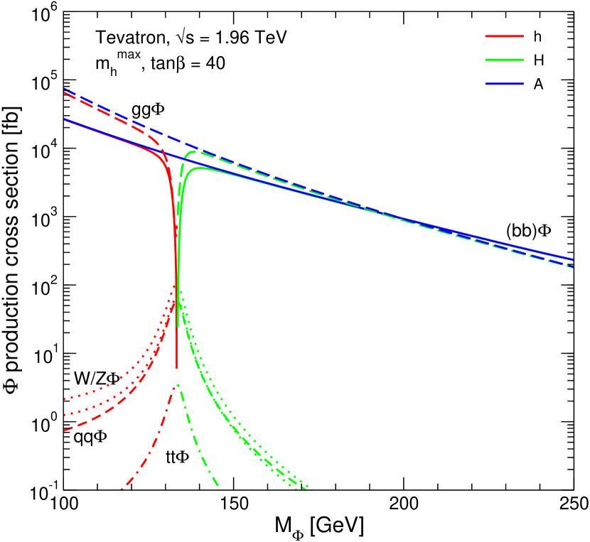
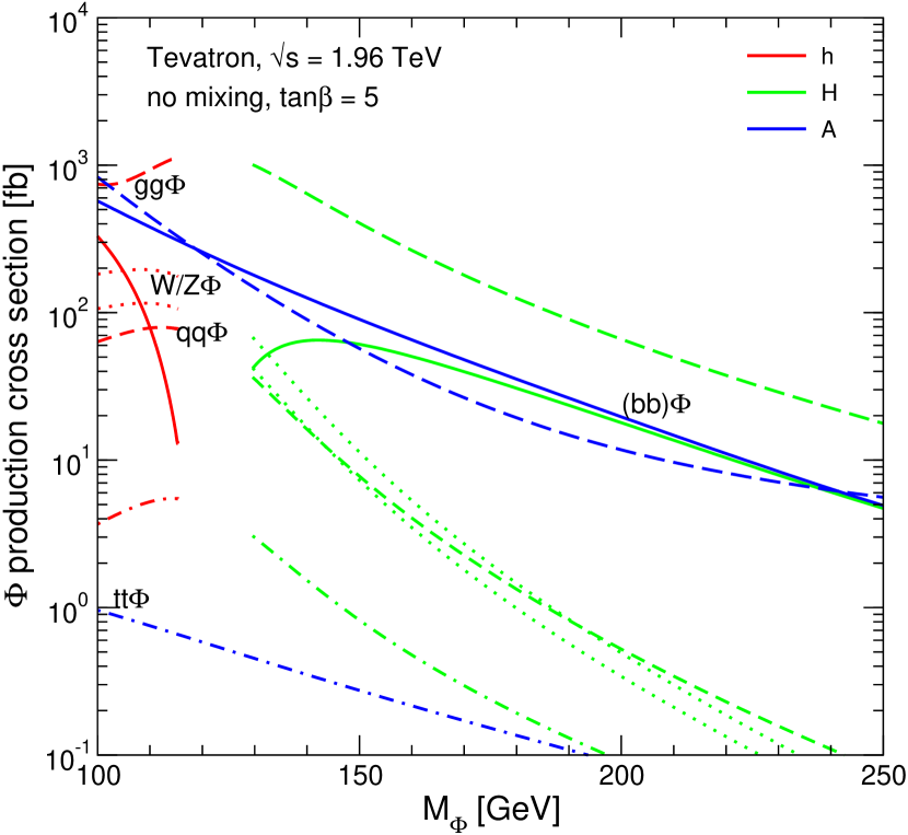
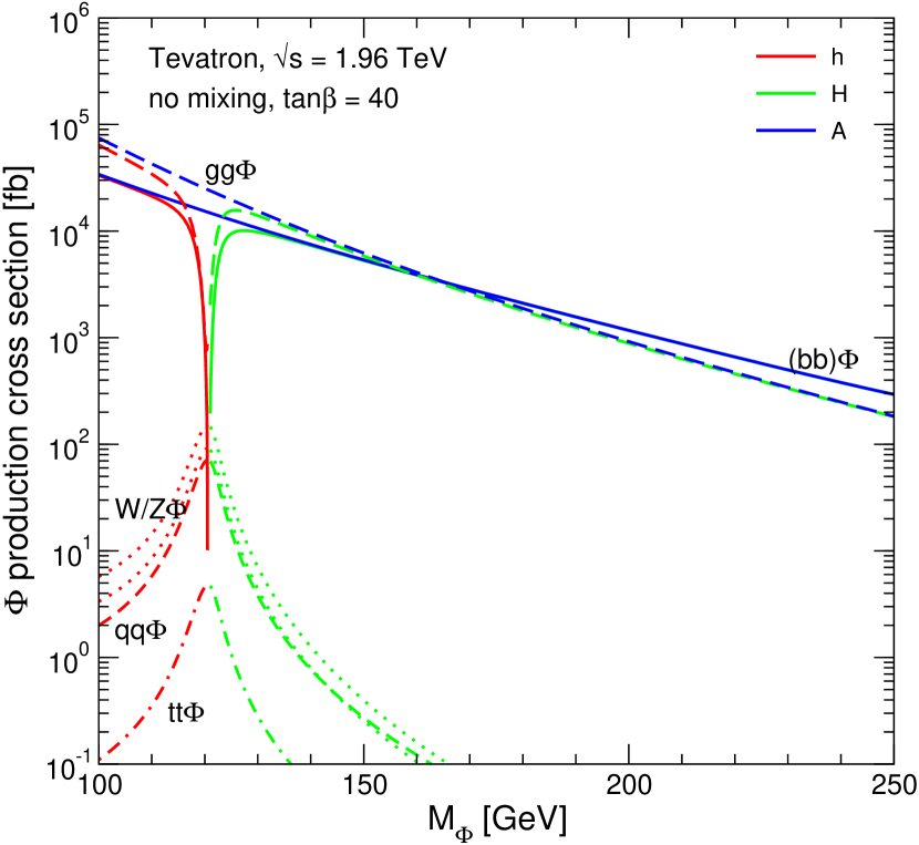
Figure 2.6.3: Neutral Higgses production cross sections (fb) at the Tevatron, $\sqrt{s}=1.96$ TeV for the most relevant production mechanims as a function of the Higgs-boson mass. Results are based on the SM cross sections and evaluated through an effective coupling approximation in the $m_{h}^{\mathrm{max}}$ and no-mixing scenarios, for $\tan\beta=5,40$.

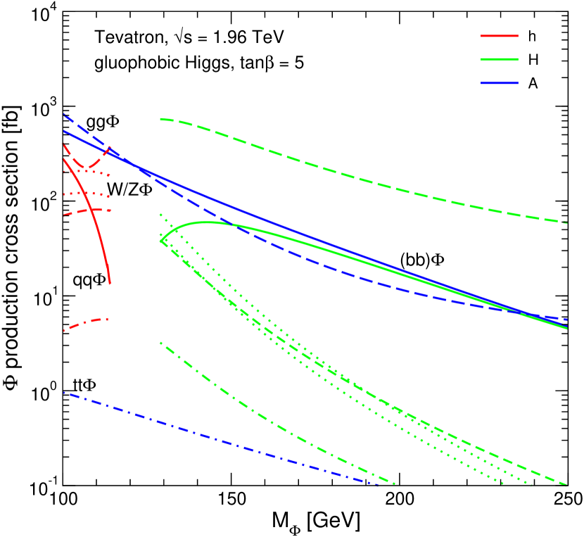
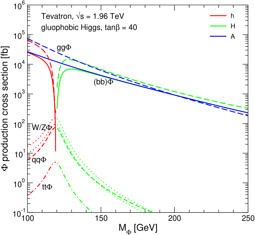
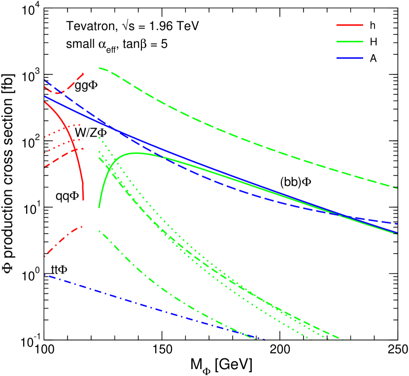
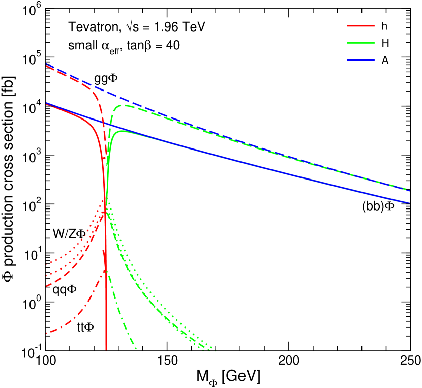
Figure 2.6.4: Same as Fig. 2.6.3, for the gluophobic Higgs and small $\alpha_{\rm eff}$ scenarios.

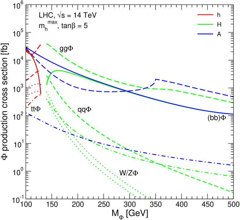
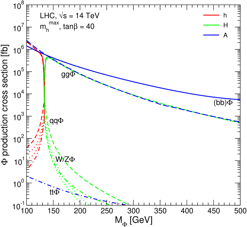
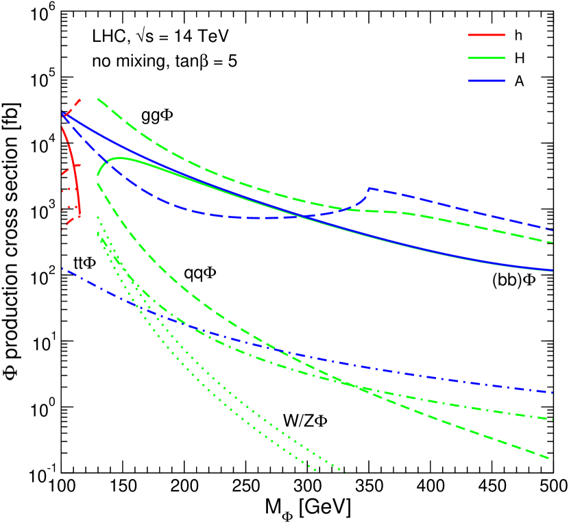
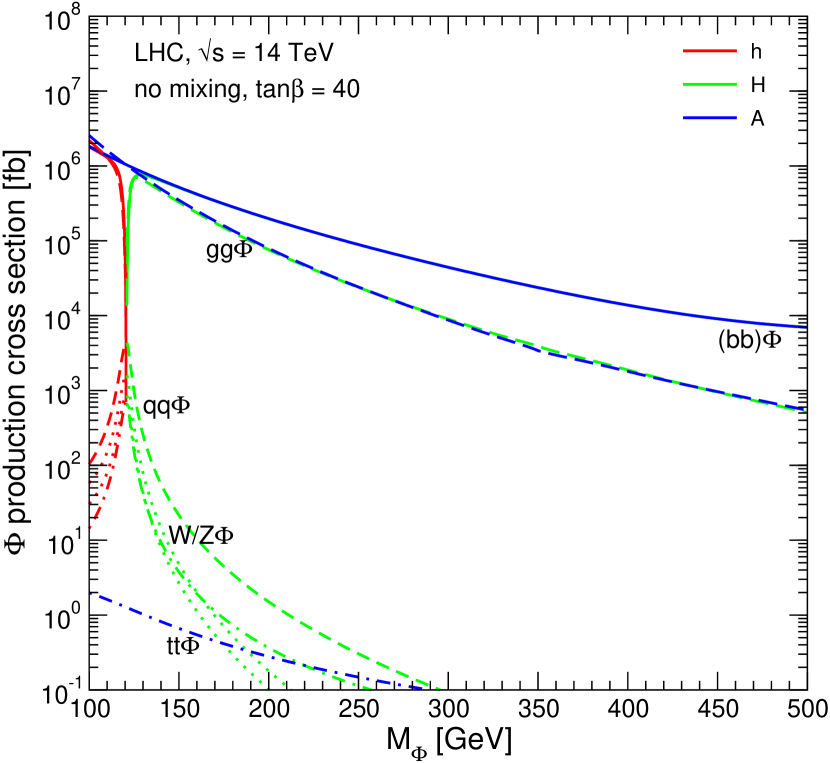
Figure 2.6.5: Neutral Higgses production cross sections (fb) at the LHC, $\sqrt{s}=14$ TeV, for the most relevant production mechanims as a function of the Higgs-boson mass. Results are based on the SM cross sections and evaluated through an effective coupling approximation in the $m_{h}^{\mathrm{max}}$ and no-mixing scenarios, for $\tan\beta=5,40$.

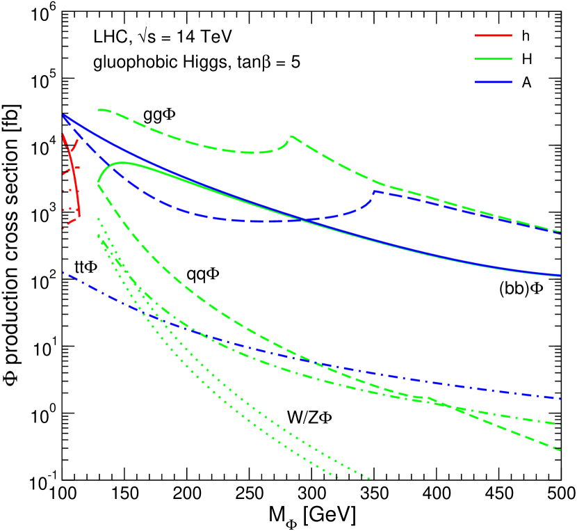
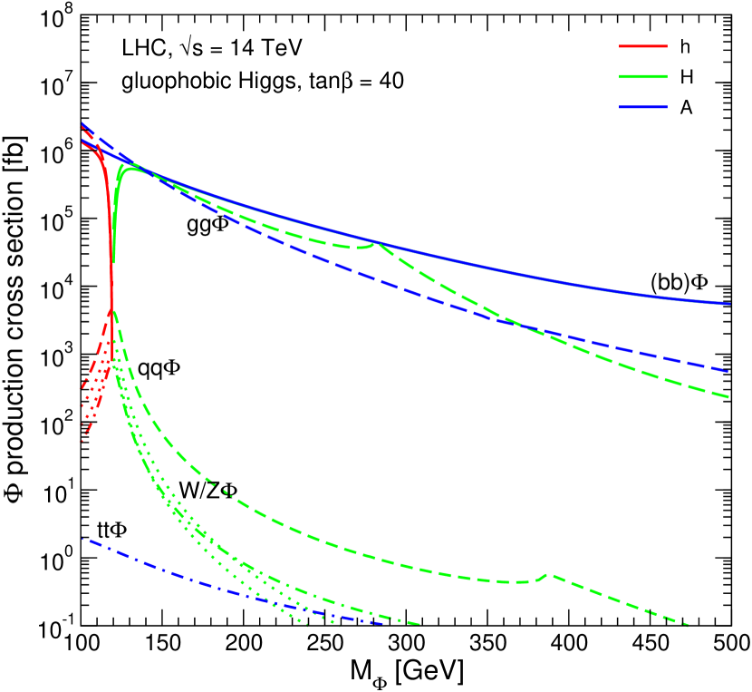
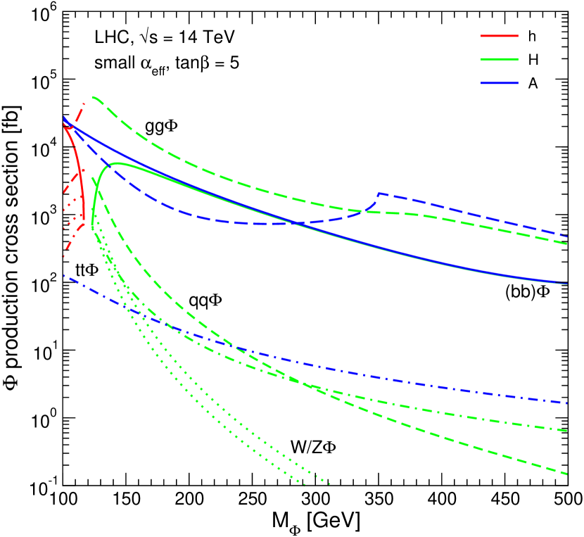
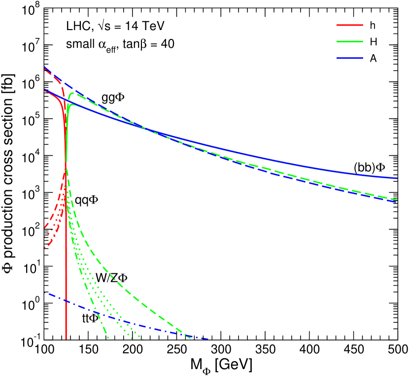
Figure 2.6.6: Same as Fig. 2.6.5, for the gluophobic Higgs and small $\alpha_{\rm eff}$ scenarios.

Acknowledgements

We are thankful to Mariano Ciccolini, Massimiliano Grazzini, Robert Harlander and Michael Krämer for making some SM predictions available to us. F.M. thanks Alessandro Vicini for useful discussions. S.H., F.M. and G.W. thank Michael Spira for lively discussions. S.H. is partially supported by CICYT (grant FPA2004-02948) and DGIID-DGA (grant 2005-E24/2).

3 Towards understanding the nature of Electroweak Symmetry Breaking at the Tevatron and LHC

Contributed by: A. Belyaev, A. Blum, S. Chivukula, E. H. Simmons
PACS 14.80.Cp,11.30.Pb,11.15.Ex

In this study we discuss how to extract information about physics beyond the Standard Model (SM) from searches for a light SM Higgs at Tevatron Run II and CERN LHC. We demonstrate that new (pseudo)scalar states predicted in both supersymmetric and dynamical models can have enhanced visibility in standard Higgs search channels, making them potentially discoverable at Tevatron Run II and CERN LHC. We discuss the likely sizes of the enhancements in the various search channels for each model and identify the model features having the largest influence on the degree of enhancement. We compare the key signals for the non-standard scalars across models and also with expectations in the SM, to show how one could start to identify which state has actually been found. In particular, we suggest the likely mass reach of the Higgs search in $p\bar{p}/pp\to{\cal H}\to\tau^{+}\tau^{-}$ for each kind of non-standard scalar state and we demonstrate that $p\bar{p}/pp\to{\cal H}\to\gamma\gamma$ may cleanly distinguish the scalars of supersymmetric models from those of dynamical models and shed the light on the pattern of Electroweak Symmetry Breaking.

3.1 Introduction

The origin of electroweak symmetry breaking remains unknown. While the Standard Model (SM) of particle physics is consistent with existing data, theoretical considerations suggest that this theory is only a low-energy effective theory and must be supplanted by a more complete description of the underlying physics at energies above those reached so far by experiment.

If the Tevatron or LHC do find evidence for a new scalar state, it may not necessarily be the Standard Higgs. Many alternative models of electroweak symmetry breaking have spectra that include new scalar or pseudoscalar states whose masses could easily lie in the range to which Run II is sensitive. The new scalars tend to have cross-sections and branching fractions that differ from those of the SM Higgs. The potential exists for one of these scalars to be more visible in a standard search than the SM Higgs would be.

Here we discuss how to extract information about non-Standard theories of electroweak symmetry breaking from searches for a light SM Higgs at Tevatron Run II and CERN LHC. Ref. [62] studied the potential of Tevatron Run II to augment its search for the SM Higgs boson by considering the process $gg\to h_{SM}\to\tau^{+}\tau^{-}$. Authors determined what additional enhancement of scalar production and branching rate, such as might be provided in a non-standard model like the MSSM, would enable a scalar to become visible in the $\tau^{+}\tau^{-}$ channel alone at Tevatron Run II. Similar work has been done for $gg\to h_{MSSM}\to\tau^{+}\tau^{-}$ at the LHC  [63] and for $gg\to h_{SM}\to\gamma\gamma$ at the Tevatron [64] and LHC [65].

Our work builds on these results, considering an additional production mechanism (b-quark annihilation), more decay channels ($b\bar{b}$, $W^{+}W^{-}$, $ZZ$, and $\gamma\gamma$), and a wider range of non-standard physics (supersymmetry and dynamical electroweak symmetry breaking) from which rate enhancement may derive. We discuss the possible sizes of the enhancements in the various search channels for each model and pinpoint the model features having the largest influence on the degree of enhancement. We suggest the mass reach of the standard Higgs searches for each kind of non-standard scalar state. We also compare the key signals for the non-standard scalars across models and also with expectations in the SM, to show how one could identify which state has actually been found. Analytic formulas for the decay widths of the SM Higgs boson are taken from [66], [67] and numerical values are calculated using the HDECAY program [68].

3.2 Models of Electroweak Symmetry Breaking

Supersymmetry

One interesting possibility for addressing the hierarchy and triviality problems of the Standard Model is to introduce supersymmetry.

In order to provide masses to both up-type and down-type quarks, and to ensure anomaly cancellation, the minimal supersymmetric Standard Model (MSSM) contains two Higgs complex-doublet superfields: $\Phi_{d}=(\Phi_{d}^{0},\Phi_{d}^{-})$ and $\Phi_{u}=(\Phi_{u}^{+},\Phi_{u}^{0})$ which aquire two vacuum expectation values $v_{1}$ and $v_{2}$ respectively. Out of the original 8 degrees of freedom, 3 serve as Goldstone bosons, absorbed into longitudinal components of the $W^{\pm}$ and $Z$, making them massive. The other 5 degrees of freedom remain in the spectrum as distinct scalar states, namely two neutral CP-even states($h$, $H$), one neutral, CP-odd state ($A$) and a charged pair ($H^{\pm}$). It is conventional to choose $\tan\beta=v_{1}/v_{2}$ and $M_{A}=\sqrt{M_{H^{\pm}}^{2}-M_{W}^{2}}$ to define the SUSY Higgs sector. There are foloowing relations between Higgs masses which will be useful for determining when Higgs boson interactions with fermions are enhanced:

$$M^{2}_{h,H}={1\over 2}\left[(M^{2}_{A}+M^{2}_{Z})\mp\sqrt{(M^{2}_{A}+M^{2}_{Z})^{2}-4M^{2}_{A}M^{2}_{Z}\cos^{2}2\beta}\right];\cos^{2}(\beta-\alpha)={M_{h}^{2}(M_{Z}^{2}-M_{h}^{2})\over M_{A}^{2}(M_{H}^{2}-M_{h}^{2})},$$ (3.2.24)

where $\alpha$ is the mixing angle of CP-even Higgs bosons. The Yukawa interactions of the Higgs fields with the quarks and leptons can be written as:

$$Y_{ht\bar{t}}/Y^{SM}_{ht\bar{t}}={\cos\alpha/\sin\beta}\ \ \ \ \ \ \ Y_{Ht\bar{t}}/Y^{SM}_{ht\bar{t}}={\sin\alpha/\sin\beta}\ \ \ \ \ \ \ Y_{At\bar{t}}/Y^{SM}_{ht\bar{t}}={\cot\beta}$$

$$Y_{hb\bar{b}}/Y^{SM}_{hb\bar{b}}={-\sin\alpha/\cos\beta}\ \ \ \ \ \ \ Y_{Hb\bar{b}}/Y^{SM}_{hb\bar{b}}={\ \cos\alpha/\cos\beta}\ \ \ \ \ \ \ Y_{Ab\bar{b}}/Y^{SM}_{hb\bar{b}}={\tan\beta}$$ (3.2.25)

relative to the Yukawa couplings of the Standard Model ($Y^{SM}_{hf\bar{f}}=m_{f}/v)$. Once again, the same pattern holds for the tau lepton’s Yukawa couplings as for those of the $b$ quark. There are several circumstances under which various Yukawa couplings are enhanced relative to Standard Model values. For high $\tan\beta$ (small $\cos\beta$), eqns. (3.2.25) show that the interactions of all neutral Higgs bosons with the down-type fermions are enhanced by a factor of $1/\cos\beta$. In the decoupling limit, where $M_{A}\to\infty$, applying eq. (3.2.24) to eqns. (3.2.25) shows that the $H$ and $A$ Yukawa couplings to down-type fermions are enhanced by a factor of $\simeq\tan\beta$. Conversely, for low $m_{A}\simeq m_{h}$, one can check that $Y_{hb\bar{b}}/Y^{SM}_{hb\bar{b}}=Y_{h\tau\bar{\tau}}/Y^{SM}_{h\tau\bar{\tau}}\simeq\tan\beta$ that $h$ and $A$ Yukawas are enhanced instead.

Technicolor

Another intriguing class of theories, dynamical electroweak symmetry breaking (DEWSB), supposes that the scalar states involved in electroweak symmetry breaking could be manifestly composite at scales not much above the electroweak scale $v\sim 250$ GeV. In these theories, a new asymptotically free strong gauge interaction (technicolor [69, 70, 71]) breaks the chiral symmetries of massless fermions $f$ at a scale $\Lambda\sim 1$ TeV. If the fermions carry appropriate electroweak quantum numbers (e.g. left-hand (LH) weak doublets and right-hand (RH) weak singlets), the resulting condensate $\langle\bar{f}_{L}f_{R}\rangle\neq 0$ breaks the electroweak symmetry as desired. Three of the Nambu-Goldstone Bosons (technipions) of the chiral symmetry breaking become the longitudinal modes of the $W$ and $Z$. The logarithmic running of the strong gauge coupling renders the low value of the electroweak scale natural. The absence of fundamental scalars obviates concerns about triviality.

Many models of DEWSB have additional light neutral pseudo Nambu-Goldstone bosons which could potentially be accessible to a standard Higgs search; these are called “technipions” in technicolor models. Our analysis will assume, for simplicity, that the lightest PNGB state is significantly lighter than other neutral (pseudo) scalar technipions, so as to heighten the comparison to the SM Higgs boson.

The specific models we examine are: 1) the traditional one-family model [72] with a full family of techniquarks and technileptons, 2) a variant on the one-family model [73] in which the lightest technipion contains only down-type technifermions and is significantly lighter than the other pseudo Nambu-Goldstone bosons, 3) a multiscale walking technicolor model [74] designed to reduce flavor-changing neutral currents, and 4) a low-scale technciolor model (the Technicolor Straw Man model) [75] with many weak doublets of technifermions, in which the second-lightest technipion $P^{\prime}$ is the state relevant for our study (the lightest, being composed of technileptons, lacks the anomalous coupling to gluons required for $gg\to P$ production). For simplicity the lightest relevant neutral technipion of each model will be generically denoted $P$; where a specific model is meant, a superscript will be used.

One of the key differences among these models is the value of the technipion decay constant $F_{P}$, which is related to the number $N_{D}$ of weak doublets of technifermions that contribute to electroweak symmetry breaking. We refer reader to [76] for details.

3.3 Results For Each Model

Supersymmetry

Let us consider how the signal of a light Higgs boson could be changed in the MSSM, compared to expectations in the SM. There are several important sources of alterations in the predicted signal, some of which are interconnected.

First, the MSSM includes three neutral Higgs bosons ${\cal H}=(h,H,A)$ states. The apparent signal of a single light Higgs could be enhanced if two or three neutral Higgs species are nearly degenerate, and we take advantage of this near-degeneracy by combining the signals of the different neutral Higgs bosons when their masses are closer than the experimental resolution.

Second, the alterations of the couplings between Higgs bosons and ordinary fermions in the MSSM can change the Higgs decay widths and branching ratios relative to those in the SM. Radiative effects on the masses and couplings can substantially alter decay branching fractions in a non-universal way. For instance, $B(h\to\tau+\tau^{-})$ could be enhanced by up to an order of magnitude due to the suppression of $B(h\to b\bar{b})$ in certain regions of parameter space [77, 78]. However, this gain in branching fraction would be offset to some degree by a reduction in Higgs production through channels involving $Y_{{\cal H}b\bar{b}}$ [62].

Third, a large value of $\tan\beta$ enhances the bottom-Higgs coupling (eqns. (3.2.25) ), making gluon fusion through a $b$-quark loop significant, and possibly even dominant over the top-quark loop contribution.

Fourth, the presence of superpartners in the MSSM gives rise to new squark-loop contributions to Higgs boson production through gluon fusion. Light squarks with masses of order 100 GeV have been argued to lead to a considerable universal enhancement (as much as a factor of five) [79, 80, 81, 82] for MSSM Higgs production compared to the SM.

Finally, enhancement of the $Y_{{\cal H}b\bar{b}}$ coupling at moderate to large $\tan\beta$ makes $b\bar{b}\to{\cal H}$ a significant means of Higgs production in the MSSM – in contrast to the SM where it is negligible. To include both production channels when looking for a Higgs decaying as ${\cal H}\to xx$, we define a combined enhancement factor

$$\kappa_{total/xx}^{\cal H}={\sigma(gg\to{\cal H}\to xx)+\sigma(bb\to{\cal H}\to xx)\over{\sigma(gg\to h_{SM}\to xx)+\sigma(bb\to h_{SM}\to xx)}}\equiv[\kappa_{gg/xx}^{\cal H}+\kappa_{bb/xx}^{\cal H}R_{bb:gg}]/[{1+R_{bb:gg}}].$$ (3.3.26)

Here $R_{bb:gg}$ is the ratio of $b\bar{b}$ and $gg$ initiated Higgs boson production in the Standard Model, which can be calculated using HDECAY.

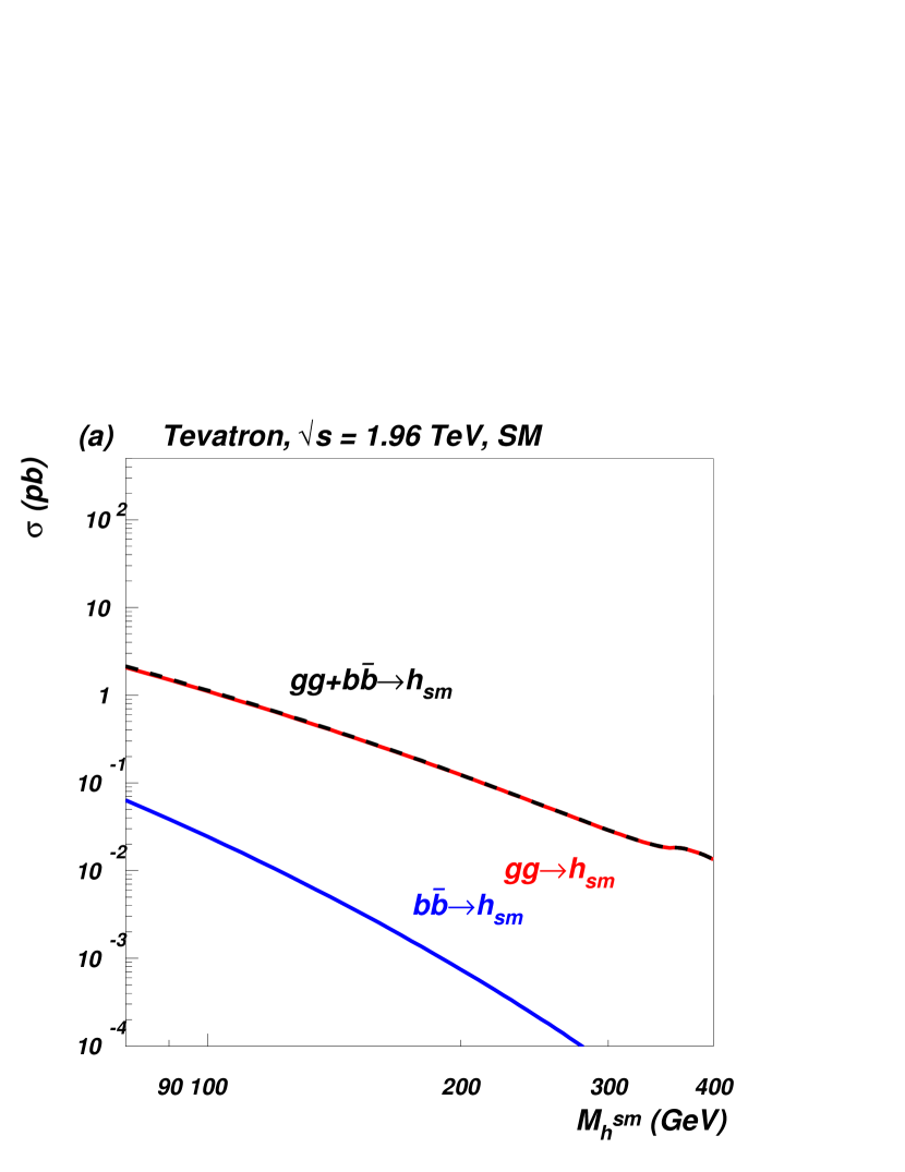
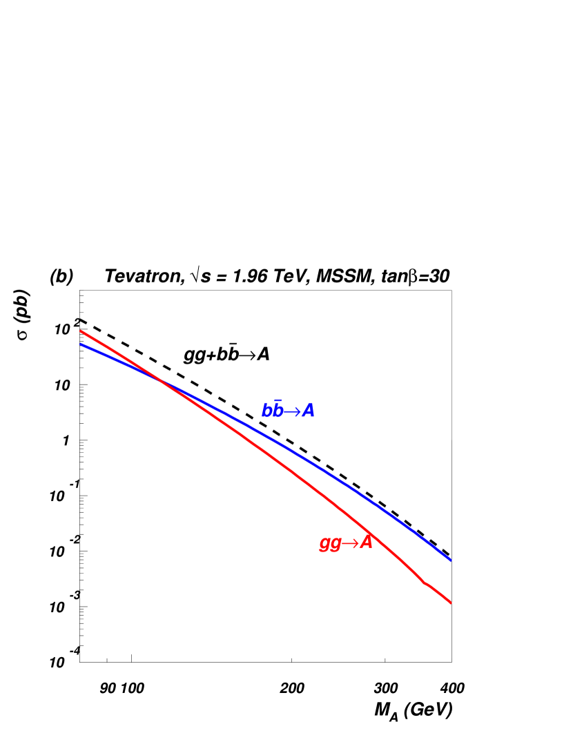
Figure 3.3.7: NLO cross sections for Higgs production via the $b\bar{b}\to{\cal H}$ and $gg\to{\cal H}$ processes (as well as their sum) at the Tevatron for the SM Higgs (a) the Supersymmetric axial Higgs boson with $\tan\beta=30$ (b).

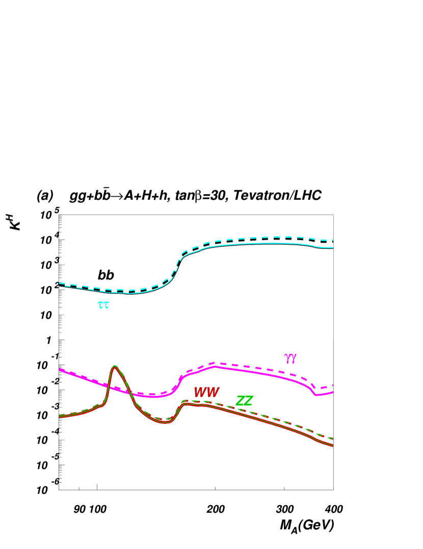
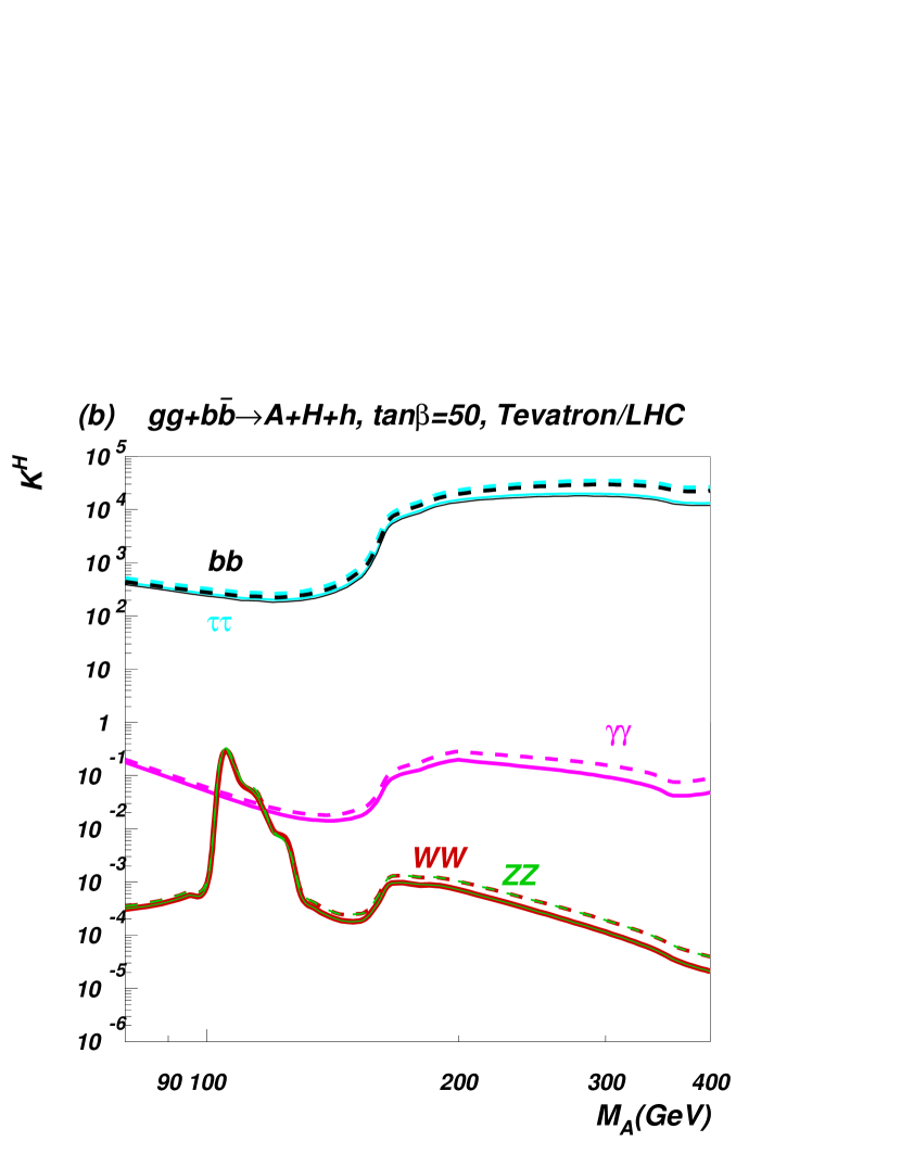
Figure 3.3.8: Enhancement factor $\kappa^{\cal H}_{tot/xx}$ for final states $xx=b\bar{b},\ \tau^{+}\tau^{-},\ WW,\ ZZ,\ \gamma\gamma$ when both $gg\to{\cal H}$ and $b\bar{b}\to{\cal H}$ are included and the signals of all three MSSM Higgs states are combined. Frames (a) and (b) correspond to $\tan\beta=30$ and 50, respectively, at the Tevatron (solid lines) and at the LHC (dashed lines).

Figure 3.3.7 presents NLO cross sections at the Tevatron. For $b\bar{b}\to{\cal H}$ we are using the code of Ref. [83], while for $gg\to{\cal H}$ we use HIGLU [84] and HDECAY [68] . One can see that in the MSSM the contribution from $b\bar{b}\to{\cal H}$ becomes important even for moderate values of $\tan\beta\sim 10$. For $M_{\cal H}<110-115$ GeV the contribution from $gg\to{\cal H}$ process is a bit bigger than that from $b\bar{b}\to{\cal H}$, while for $M_{\cal H}>115$ GeV $b$-quark-initiated production begins to outweigh gluon-initiated production. Results for LHC are qualitatively similar, except the rate, which is about two orders of magnitude higher compared to that at the Tevatron.

Using the Higgs branching fractions with these NLO cross sections for $gg\to H$ and $b\bar{b}\to H$ allows us to derive $\kappa_{total/xx}^{\cal H}$, as presented in Fig. 3.3.8 for the Tevatron and LHC. There are several “physical” kinks and peaks in the enhancement factor for various Higgs boson final states related to $WW$, $ZZ$ and top-quark thresholds which can be seen for the respective values of $M_{A}$. At very large values of $\tan\beta$ the top-quark threshold effect for the $\gamma\gamma$ enhancement factor is almost gone because the b-quark contribution dominates in the loop. One can see from Fig. 3.3.8 that the enhancement factors at the Tevatron and LHC are very similar. On the other hand, the values of the total rates at the LHC are about two orders of magnitude higher than the corresponding rates at the Tevatron. In contrast to strongly enhanced $b\bar{b}$ and $\tau\bar{\tau}$ signatures, the $\gamma\gamma$ signature is always strongly suppressed! This particular feature of SUSY models, as we will see below, may be important for distinguishing supersymmetric models from models with dynamical symmetry breaking.

It is important to note that combining the signal from the neutral Higgs bosons $h,A,H$ in the MSSM turns out to make our results more broadly applicable across SUSY parameter space. Combining the signals from $A,h,H$ has the virtue of making the enhancement factor independent of the degree of top squark mixing (for fixed $M_{A}$, $\mu$ and $M_{S}$ and medium to high values of $\tan\beta$), which greatly reduces the parameter-dependence of our results.

Technicolor

Single production of a technipion can occur through the axial-vector anomaly which couples the technipion to pairs of gauge bosons. For an $SU(N_{TC})$ technicolor group with technipion decay constant $F_{P}$, the anomalous coupling between the technipion and a pair of gauge bosons is given, in direct analogy with the coupling of a QCD pion to photons, by [85, 86, 87]. Comparing a PNGB to a SM Higgs boson of the same mass, we find the enhancement in the gluon fusion production is

$$\kappa_{gg\ prod}=\frac{\Gamma(P\rightarrow gg)}{\Gamma(h\rightarrow gg)}=\frac{9}{4}N_{TC}^{2}{\cal A}_{gg}^{2}\frac{v^{2}}{F_{P}^{2}}$$ (3.3.27)

The main factors influencing $\kappa_{gg\ prod}$ for a fixed value of $N_{TC}$ are the anomalous coupling to gluons and the technipion decay constant. The value of $\kappa_{gg\ prod}$ for each model (taking $N_{TC}=4$) is given in Table 3.3.1.

Table 3.3.1: Calculated enhancement factors for production at the Tevatron and LHC of a 130 GeV technipion via $gg$ alone, via $b\bar{b}$ alone, and combined. Note that the small enhancement in the $b\bar{b}$ process slightly reduces the total enhancement relative to that of $gg$ alone. In all cases, $N_{TC}=4$.

	1) one family	2) variant one-family	3) multiscale	4) low scale
$\kappa^{P}_{gg\ prod}$	48	6	1200	120
$\kappa^{P}_{bb\ prod}$	4	0.67	16	10
$\kappa^{P}_{prod}$	47	5.9	1100	120

The value of $\kappa_{bb\ prod}$ (shown in Table 3.3.1) is controlled by the size of the technipion decay constant.

We see from Table 3.3.1 that $\kappa_{bb\ prod}$ is at least one order of magnitude smaller than $\kappa_{gg\ prod}$ in each model. From the ${\kappa_{gg\ prod}}/{\kappa_{bb\ prod}}$ ratio which reads as

$$\frac{\kappa_{gg\ prod}}{\kappa_{bb\ prod}}=\frac{9}{4}N_{TC}^{2}{\cal A}_{gg}^{2}\lambda_{b}^{-2}\left(1-\frac{4m_{b}^{2}}{m_{h}^{2}}\right)^{\frac{3-s}{2}},$$ (3.3.28)

we see that the larger size of $\kappa_{gg\ prod}$ is due to the factor of $N_{TC}^{2}$ coming from the fact that gluons couple to a technipion via a techniquark loop. The extended technicolor (ETC) interactions coupling $b$-quarks to a technipion have no such enhancement. With a smaller SM cross-section and a smaller enhancement factor, it is clear that technipion production via $b\bar{b}$ annihilation is essentially negligible at these hadron colliders.

We now calculate the technipion branching ratios from the above information, taking $N_{TC}=4$. The values are essentially independent of the size of $M_{P}$ within the range 120 GeV - 160 GeV; the branching fractions for $M_{P}=130$ GeV are shown in Table 3.3.2. The branching ratios for the SM Higgs at NLO are given for comparison; they were calculated using HDECAY [68].

Table 3.3.2: Branching ratios of Technipions/Higgs of mass 130 GeV

Decay	1) one family	2) variant	3) multiscale	4) low scale	SM Higgs
Channel		one family
$b\overline{b}$	0.60	0.53	0.23	0.60	0.53
$\tau^{+}\tau^{-}$	0.03	0.25	0.01	0.03	0.05
$\gamma\gamma$	$2.7\times 10^{-4}$	$2.9\times 10^{-3}$	$6.1\times 10^{-4}$	$6.4\times 10^{-3}$	$2.2\times 10^{-3}$

Comparing the technicolor and SM branching ratios in Table 3.3.2, we see immediately that all decay enhancements. Model 2 is an exception; its unusual Yukawa couplings yield a decay enhancement in the $\tau^{+}\tau^{-}$ channel of order the technipion’s (low) production enhancement. In the $\gamma\gamma$ channel, the decay enhancement strongly depends on the group-theoretical structure of the model, through the anomaly factor.

Table 3.3.3: Enhancement Factors for 130 GeV technipions produced at the Tevatron and LHC, compared to production and decay of a SM Higgs Boson of the same mass. The slight suppression of $\kappa^{P}_{prod}$ due to the b-quark annihilation channel has been included. The rightmost column shows the cross-section (pb) for $p\bar{p}/pp\to P\to xx$ at Tevatron Run II/LHC.

Model	Decay mode	$\kappa^{P}_{prod}$	$\kappa^{P}_{dec}$	$\kappa^{P}_{tot/xx}$	$\sigma$(pb) Tevatron/LHC
	$b\overline{b}$	47	1.1	52	14 / 890
1) one family	$\tau^{+}\tau^{-}$	47	0.6	28	0.77 / 48
	$\gamma\gamma$	47	0.12	5.6	$6.4\times 10^{-3}$ / 0.4
	$b\overline{b}$	5.9	1	5.9	1.8 / 100
2) variant	$\tau^{+}\tau^{-}$	5.9	5	30	0.84 / 52
one family	$\gamma\gamma$	5.9	1.3	7.7	$8.7\times 10^{-3}$ / 0.55
	$b\overline{b}$	1100	0.43	470	130 / 8000
3) multiscale	$\tau^{+}\tau^{-}$	1100	0.2	220	6.1 / 380
	$\gamma\gamma$	1100	0.27	300	0.34 /22

Our results for the Tevatron Run II and LHC production enhancements (including both $gg$ fusion and $b\bar{b}$ annihilation), decay enhancements, and overall enhancements of each technicolor model relative to the SM are shown in Table  3.3.3 for a technipion or Higgs mass of 130 GeV. Multiplying $\kappa^{P}_{tot/xx}$ by the cross-section for SM Higgs production via gluon fusion [84] yields an approximate technipion production cross-section, as shown in the right-most column of Table 3.3.3.

In each technicolor model, the main enhancement of the possible technipion signal relative to that of an SM Higgs arises at production, making the size of the technipion decay constant the most critical factor in determining the degree of enhancement for fixed $N_{TC}$.

3.4 Interpretation

We are ready to put our results in context. The large QCD background for $q\bar{q}$ states of any flavor makes the tau-lepton-pair and di-photon final states the most promising for exclusion or discovery of the Higgs-like states of the MSSM or technicolor. We now illustrate how the size of the enhancement factors for these two final states vary over the parameter spaces of these theories at the Tevatron and LHC. We use this information to display the likely reach of each experiment in each of these standard Higgs search channels. Then, we compare the signatures of the MSSM Higgs bosons and the various technipions to see how one might tell these states apart from one another.

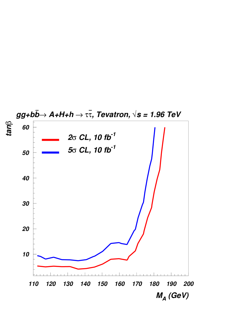
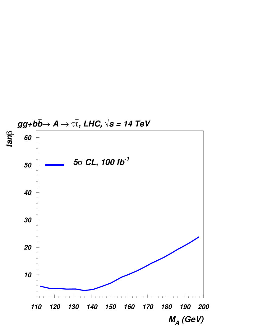
Figure 3.4.9: Results for $gg+b\bar{b}\to h+H+A\to\tau^{+}\tau^{-}$ at LHC. Left frame: Selected contours of given enhancement factor values $\kappa^{\cal H}_{total/\tau\tau}$ in the MSSM. Right frame: Predicted LHC reach, based on the $h_{SM}\to\tau^{+}\tau^{-}$ studies of [63], in the MSSM parameter space.

In of Figure 3.4.9 we summarize the ability of Tevatron (left) and LHC (right) to explore the MSSM parameter space (in terms of both a $2\sigma$ exclusion curve and a $5\sigma$ discovery curve) using the process $gg+b\bar{b}\to h+A+H\to\tau^{+}\tau^{-}$. Translating the enhancement factors into this reach plot draws on the results of [62]. As the $M_{A}$ mass increases up to about 140 GeV, the opening of the $W^{+}W^{-}$ decay channel drives the $\tau^{+}\tau^{-}$ branching fraction down, and increases the $\tan\beta$ value required to make Higgses visible in the $\tau^{+}\tau^{-}$ channel. At still larger $M_{A}$, a very steep drop in the gluon luminosity (and the related $b$-quark luminosity) at large $x$ reduces the phase space for ${\cal H}$ production. Therefore for $M_{A}>$170 GeV, Higgs bosons would only be visible at very high values of $\tan\beta$. The pictures for tevaron and LHC are qualitatively similar, the main differences compared to the Tevatron are that the required value of $\tan\beta$ at the LHC is lower for a given $M_{A}$ and it does not climb steeply for $M_{A}>$170 GeV because there is much less phase space suppression.

It is important to notice that both, Tevatron and LHC, could observe MSSM Higgs bosons in the $\tau^{+}\tau^{-}$ channel even for moderate values of $\tan\beta$ for $M_{A}\lesssim 200$ GeV, because of significant enhancement of this channel. However the $\gamma\gamma$ channel is so suppressed that even the LHC will not be able to observe it in any point of the $M_{A}<200$ GeV parameter space studied in this paper!

The Figure 3.4.10 presents the Tevatron and LHC potentials to observe technipions. For the Tevatron, the observability is presented in terms of enhancement factor, while for the LHC we present signal rate in term of $\sigma\times Br(P\to\tau\tau/\gamma\gamma)$. At the Tevatron, the available enhancement is well above what is required to render the $P$ of any of these models visible in the $\tau^{+}\tau^{-}$ channel. Likewise, the right frame of that figure shows that in the $\gamma\gamma$ channel at the Tevatron the technipions of models 3 and 4 will be observable at the $5\sigma$ level while model 2 is subject to exclusion at the $2\sigma$ level. The situation at the LHC is even more promising: all four models could be observable at the $5\sigma$ level in both the $\tau^{+}\tau^{-}$ (left frame) and $\gamma\gamma$ (right frame) channels.

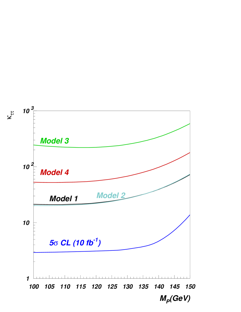
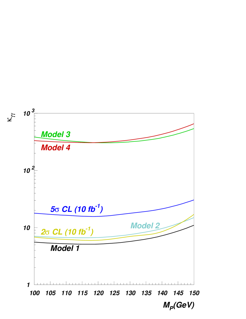
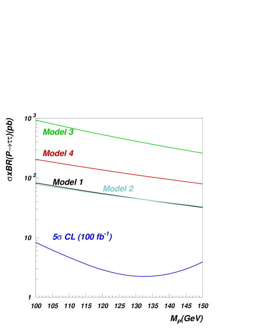
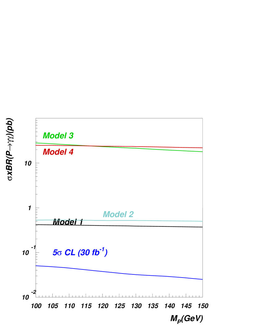
Figure 3.4.10: Observability of technipions as a function of technipion mass and assuming the final state is a tau pair (left frame) or photon pair (right frame) at the Tveatron and LHC. Top raw: the $5\sigma$ discovery and $2\sigma$ exclusion curves indicate the required enhancement factor for a Higgs-like particle at Tevatron Run II when the final state is $\tau^{+}\tau^{-}$ [62] (left frame) or $\gamma\gamma$ [64](right frame). Bottom raw: the lowest curve is the $\sigma\times Br$ required to make a Higgs-like particle visible ($5\sigma$ discovery) in $\tau^{+}\tau^{-}$ [63] or in $\gamma\gamma$ [65] at LHC.

Once a supposed light “Higgs boson” is observed in a collider experiment, an immediate important task will be to identify the new state more precisely, i.e. to discern “the meaning of Higgs” in this context. Comparison of the enhancement factors for different channels will aid in this task. Our study has shown that comparison of the $\tau^{+}\tau^{-}$ and $\gamma\gamma$ channels can be particularly informative in distinguishing supersymmetric from dynamical models. In the case of supersymmetry, when the $\tau^{+}\tau^{-}$ channel is enhanced, the $\gamma\gamma$ channel is suppressed, and this suppression is strong enough that even the LHC would not observe the $\gamma\gamma$ signature. In contrast, for the dynamical symmetry breaking models studied we expect simultaneous enhancement of both the $\tau^{+}\tau^{-}$ and $\gamma\gamma$ channels. The enhancement of the $\gamma\gamma$ channel is so significant, that even at the Tevatron we may observe technipions via this signature at the $5\sigma$ level for Models 3 and 4, while Model 2 could be excluded at 95% CL at the Tevatron. The LHC collider, which will have better sensitivity to the signatures under study, will be able to observe all four models of dynamical symmetry breaking studied here in the $\gamma\gamma$ channel, and can therefore distinguish more conclusively between the supersymmetric and dynamical models.

3.5 Conclusions

In this paper we have shown that searches for a light Standard Model Higgs boson at Tevatron Run II and CERN LHC have the power to provide significant information about important classes of physics beyond the Standard Model. We demonstrated that the new scalar and pseudo-scalar states predicted in both supersymmetric and dynamical models can have enhanced visibility in standard $\tau^{+}\tau^{-}$ and $\gamma\gamma$ search channels, making them potentially discoverable at both the Tevatron Run II and the CERN LHC. In comparing the key signals for the non-standard scalars across models we investigated the likely mass reach of the Higgs search in $pp/p\bar{p}\to{\cal H}\to\tau^{+}\tau^{-}$ for each kind of non-standard scalar state, and we demonstrated that $pp\,\ \,p\bar{p}\to{\cal H}\to\gamma\gamma$ may cleanly distinguish the scalars of supersymmetric models from those of dynamical models.

Acknowledgments

This work was supported in part by the U.S. National Science Foundation under awards PHY-0354838 (A. Belyaev) and PHY-0354226 (R. S. Chivukula and E. H. Simmons). A.B. thanks organizers of Tev4LHC workshop for the creative atmosphere and hospitality.

4 MSSM Higgs Boson Searches at the Tevatron and the LHC: Impact of Different Benchmark Scenarios

Contributed by: M. Carena, S. Heinemeyer, C.E.M. Wagner, G. Weiglein

The MSSM requires two Higgs doublets, resulting in five physical Higgs boson degrees of freedom. These are the light and heavy $\mathcal{C}P$-even Higgs bosons, $h$ and $H$, the $\mathcal{C}P$-odd Higgs boson, $A$, and the charged Higgs boson, $H^{\pm}$. The Higgs sector of the MSSM can be specified at lowest order in terms of $M_{Z}$, $M_{A}$, and $\tan\beta\equiv v_{2}/v_{1}$, the ratio of the two Higgs vacuum expectation values. The masses of the $\mathcal{C}P$-even neutral Higgs bosons and the charged Higgs boson can be calculated, including higher-order corrections, in terms of the other MSSM parameters.

After the termination of LEP in the year 2000 (the close-to-final LEP results can be found in Refs. [6, 47]), the Higgs boson search has shifted to the Tevatron and will later be continued at the LHC. Due to the large number of free parameters, a complete scan of the MSSM parameter space is too involved. Therefore the search results at LEP have been interpreted [47] in several benchmark scenarios [52, 53]. Current analyses at the Tevatron and investigations of the LHC [51] potential also have been performed in the scenarios proposed in Refs. [52, 53]. The $m_{h}^{\mathrm{max}}$ scenario has been used to obtain conservative bounds on $\tan\beta$ for fixed values of the top-quark mass and the scale of the supersymmetric particles [58]. These scenarios are conceived to study particular cases of challenging and interesting phenomenology in the searches for the SM-like Higgs boson, i.e. mostly the light $\mathcal{C}P$-even Higgs boson.

The current searches at the Tevatron are not yet sensitive to a SM-like Higgs in the mass region allowed by the LEP exclusion bounds [6, 47]. On the other hand, scenarios with enhanced Higgs boson production cross sections can be probed already with the currently accumulated luminosity. Enhanced production cross sections can occur in particular for low $M_{A}$ in combination with large $\tan\beta$ due to the enhanced couplings of the Higgs bosons to down-type fermions. The corresponding limits on the Higgs production cross section times branching ratio of the Higgs decay into down-type fermions can be interpreted in MSSM benchmark scenarios. Limits from Run II of the Tevatron have recently been published for the following channels [88, 89, 50] (here and in the following $\phi$ denotes all three neutral MSSM Higgs bosons, $\phi=h,H,A$):

$$b\bar{b}\phi,\phi\to b\bar{b}~{}(\mbox{with one additional tagged }b\mbox{ jet}),$$ (4.0.29)

$$p\bar{p}\to\phi\to\tau^{+}\tau^{-}~{}(\mbox{inclusive}),$$ (4.0.30)

$$p\bar{p}\to t\bar{t}\to H^{\pm}W^{\mp}\,b\bar{b},H^{\pm}\to\tau\nu_{\tau}~{}.$$ (4.0.31)

The obtained cross section limits have been interpreted in the $m_{h}^{\mathrm{max}}$ and the no-mixing scenario with a value for the higgsino mass parameter of $\mu=-200\mathrm{\ Ge\kern-1.00006ptV}$ [88] and $\mu=\pm 200\mathrm{\ Ge\kern-1.00006ptV}$ [89]. In these scenarios for $M_{A}\approx 100\mathrm{\ Ge\kern-1.00006ptV}$ the limits on $\tan\beta$ are $\tan\beta\mathrel{\raise 1.29167pt\hbox{$<$\kern-7.5pt\lower 4.30554pt\hbox{$\sim$}}}50$.

Here we investigate the dependence of the CDF and D0 exclusion bounds in the $M_{A}$–$\tan\beta$ plane on the parameters entering through the most relevant supersymmetric radiative corrections in the theoretical predictions for Higgs boson production and decay processes. We will show that the bounds obtained from the $b\bar{b}\phi,\phi\to b\bar{b}$ channel depend very sensitively on the radiative corrections affecting the relation between the bottom quark mass and the bottom Yukawa coupling. In the channels with $\tau^{+}\tau^{-}$ final states, on the other hand, compensations between large corrections in the Higgs production and the Higgs decay occur. In this context we investigate the impact of a large radiative correction in the $gg\to\phi$ production process that had previously been omitted.

In order to reflect the impact of the corrections to the bottom Yukawa coupling on the exclusion bounds we suggest to supplement the existing $m_{h}^{\mathrm{max}}$  and no-mixing scenarios, mostly designed to search for the light $\mathcal{C}P$-even MSSM Higgs boson, $h$, with additional values for the higgsino mass parameter $\mu$. In fact, varying the value and sign of $\mu$, while keeping fixed the values of the gluino mass and the common third generation squark mass parameter $M_{\mathrm{SUSY}}$, demonstrates the effect of the radiative corrections on the production and decay processes. The scenarios discussed here are designed specifically to study the MSSM Higgs sector without assuming any particular soft supersymmetry-breaking scenario and taking into account constraints only from the Higgs boson sector itself. In particular, constraints from requiring the correct cold dark matter density, ${\rm BR}(b\to s\gamma)$ or $(g-2)_{\mu}$, which depend on other parameters of the theory, are not crucial in defining the Higgs boson sector, and may be avoided.

We also study the non-standard MSSM Higgs boson search sensitivity at the LHC, focusing on the processes $pp\to H/A+X,\,H/A\to\tau^{+}\tau^{-}$ and $pp\to tH^{\pm}+X,\,H^{\pm}\to\tau\nu_{\tau}$, and stress the relevance of the proper inclusion of supersymmetric radiative corrections to the production cross sections and decay widths. We show the impact of these corrections by investigating the variation of the Higgs boson discovery reach in the benchmark scenarios for different values of $\mu$. In particular, we discuss the resulting modification of the parameter region in which only the light $\mathcal{C}P$-even MSSM Higgs boson can be detected at the LHC.

4.1 Predictions for Higgs boson production and decay processes

Notation and renormalization

The tree-level values for the $\mathcal{C}P$-even Higgs bosons of the MSSM, $m_{h}$ and $m_{H}$, are determined by $\tan\beta$, the $\mathcal{C}P$-odd Higgs-boson mass $M_{A}$, and the $Z$ boson mass $M_{Z}$. The mass of the charged Higgs boson, $m_{H^{\pm}}$, is given in terms of $M_{A}$ and the $W$ boson mass, $M_{W}$. Beyond the tree-level, the main correction to the Higgs boson masses stems from the $t/\tilde{t}$ sector, and for large values of $\tan\beta$ also from the $b/\tilde{b}$ sector.

In order to fix our notations, we list the conventions for the inputs from the scalar top and scalar bottom sector of the MSSM: the mass matrices in the basis of the current eigenstates $\tilde{t}_{L},\tilde{t}_{R}$ and $\tilde{b}_{L},\tilde{b}_{R}$ are given by (modulo numerically small $D$-term contributions)

$${\cal M}^{2}_{\tilde{t}}=\left(\begin{array}[]{cc}M_{\tilde{t}_{L}}^{2}+m_{t}^{2}&m_{t}X_{t}\\ m_{t}X_{t}&M_{\tilde{t}_{R}}^{2}+m_{t}^{2}\end{array}\right),\quad{\cal M}^{2}_{\tilde{b}}=\left(\begin{array}[]{cc}M_{\tilde{b}_{L}}^{2}+m_{b}^{2}&m_{b}X_{b}\\ m_{b}X_{b}&M_{\tilde{b}_{R}}^{2}+m_{b}^{2}\end{array}\right),$$ (4.1.32)

where

$$m_{t}X_{t}=m_{t}(A_{t}-\mu\cot\beta),\quad m_{b}\,X_{b}=m_{b}\,(A_{b}-\mu\tan\beta).$$ (4.1.33)

Here $A_{t}$ denotes the trilinear Higgs–stop coupling, $A_{b}$ denotes the Higgs–sbottom coupling, and $\mu$ is the higgsino mass parameter. SU(2) gauge invariance leads to the relation $M_{\tilde{t}_{L}}=M_{\tilde{b}_{L}}$ . For the numerical evaluation, a convenient choice is

$$M_{\tilde{t}_{L}}=M_{\tilde{b}_{L}}=M_{\tilde{t}_{R}}=M_{\tilde{b}_{R}}=:M_{\mathrm{SUSY}}.$$ (4.1.34)

The Higgs sector observables furthermore depend on the SU(2) gaugino mass parameter, $M_{2}$. The other gaugino mass parameter, $M_{1}$, is usually fixed via the GUT relation $M_{1}=\frac{5}{3}\frac{s_{\mathrm{w}}^{2}}{c_{\mathrm{w}}^{2}}M_{2}$. At the two-loop level also the gluino mass, $m_{\tilde{g}}$, enters the predictions for the Higgs-boson masses.

Corrections to the MSSM Higgs boson sector have been evaluated in several approaches. The status of the available corrections to the masses and mixing angles in the MSSM Higgs sector (with real parameters) can be summarized as follows. For the one-loop part, the complete result within the MSSM is known [90, 91]. The by far dominant one-loop contribution is the ${\cal O}(\alpha_{t})$ term due to top and stop loops ($\alpha_{t}\equiv h_{t}^{2}/(4\pi)$, $h_{t}$ being the top-quark Yukawa coupling). Concerning the two-loop effects, their computation is quite advanced and has now reached a stage such that all the presumably dominant contributions are known [92, 93, 94, 95, 96, 7, 97, 98, 99, 100, 101, 102, 103, 104, 105, 106, 107, 108, 109, 110]. The remaining theoretical uncertainty on the light $\mathcal{C}P$-even Higgs boson mass has been estimated to be below $\sim 3\mathrm{\ Ge\kern-1.00006ptV}$ [8, 111]. The above calculations have been implemented into public codes. The program FeynHiggs [55, 112] is based on the results obtained in the Feynman-diagrammatic (FD) approach [7, 8, 110]. It includes all the above corrections. The code CPsuperH [113] is based on the renormalization group (RG) improved effective potential approach [93, 94, 95, 96, 114]. For the MSSM with real parameters the two codes can differ by up to $\sim 4\mathrm{\ Ge\kern-1.00006ptV}$ for the light $\mathcal{C}P$-even Higgs boson mass, mostly due to formally subleading two-loop corrections that are included only in FeynHiggs.

It should be noted in this context that the FD result has been obtained in the on-shell (OS) renormalization scheme, whereas the RG result has been calculated using the $\overline{\rm{MS}}$ scheme; see Refs. [114, 115] for a detailed comparison. Owing to the different schemes used in the FD and the RG approach for the renormalization in the scalar top sector, the parameters $X_{t}$ and $M_{\mathrm{SUSY}}$ are also scheme-dependent in the two approaches.

Leading effects from the bottom/sbottom sector

The relation between the bottom-quark mass and the Yukawa coupling $h_{b}$, which controls also the interaction between the Higgs fields and the sbottom quarks, is affected at one-loop order by large radiative corrections [105, 106, 107, 108, 109]. The leading effects are included in the effective Lagrangian formalism developed in Ref. [108]. Numerically this is by far the dominant part of the contributions from the sbottom sector (see also Refs. [103, 110, 104]). The effective Lagrangian is given by

$$\cal L=\frac{g}{2M_{W}missing}\frac{\overline{m}_{b}missing}{1+\Delta_{b}}\Bigg{[} \tan\beta\;A\,i\,\bar{b}\gamma_{5}b+\sqrt{2}\,V_{tb}\,\tan\beta\;H^{+}\bar{t}_{L}b_{R}$$

$$+ \left(\frac{\sin\alpha}{\cos\beta}-\Delta_{b}\frac{\cos\alpha}{\sin\beta}\right)h\bar{b}_{L}b_{R}-\left(\frac{\cos\alpha}{\cos\beta}+\Delta_{b}\frac{\sin\alpha}{\sin\beta}\right)H\bar{b}_{L}b_{R}\Bigg{]}+{\rm h.c.}~{}.$$

Here $\overline{m}_{b}$ denotes the running bottom quark mass including SM QCD corrections. In the numerical evaluations obtained with FeynHiggs below we choose $\overline{m}_{b}=\overline{m}_{b}(m_{t})\approx 2.97\mathrm{\ Ge\kern-1.00006ptV}$. The prefactor $1/(1+\Delta_{b})$ in Equation 4.1 arises from the resummation of the leading corrections to all orders. The additional terms $\sim\Delta_{b}$ in the $h\bar{b}b$ and $H\bar{b}b$ couplings arise from the mixing and coupling of the “other” Higgs boson, $H$ and $h$, respectively, to the $b$ quarks.

As explained above, the function $\Delta_{b}$ consists of two main contributions, an ${\cal O}(\alpha_{s})$ correction from a sbottom–gluino loop and an ${\cal O}(\alpha_{t})$ correction from a stop–higgsino loop. The explicit form of $\Delta_{b}$ in the limit of $M_{S}\gg m_{t}$ and $\tan\beta\gg 1$ reads [105, 106, 107]

$$\Delta_{b}=\frac{2\alpha_{s}}{3\,\pi}\,m_{\tilde{g}}\,\mu\,\tan\beta\,\times\,I(m_{\tilde{b}_{1}},m_{\tilde{b}_{2}},m_{\tilde{g}})+\frac{\alpha_{t}}{4\,\pi}\,A_{t}\,\mu\,\tan\beta\,\times\,I(m_{\tilde{t}_{1}},m_{\tilde{t}_{2}},\mu)~{}.$$ (4.1.36)

The function $I$ is given by

$$I(a,b,c) = \frac{1}{(a^{2}-b^{2})(b^{2}-c^{2})(a^{2}-c^{2})}\,\left(a^{2}b^{2}\log\frac{a^{2}}{b^{2}}+b^{2}c^{2}\log\frac{b^{2}}{c^{2}}+c^{2}a^{2}\log\frac{c^{2}}{a^{2}}\right)$$

$$\sim \frac{1}{\mbox{max}(a^{2},b^{2},c^{2})}~{}.$$

The large $\tilde{b}-\tilde{g}$ loops are resummed to all orders of $(\alpha_{s}\tan\beta)^{n}$ via the inclusion of $\Delta_{b}$ [105, 106, 107, 108, 109]. The leading electroweak contributions are taken into account via the second term in Equation 4.1.36.

For large values of $\tan\beta$ and the ratios of $\mu m_{\tilde{g}}/M_{\mathrm{SUSY}}^{2}$ and $\mu A_{t}/M_{\mathrm{SUSY}}^{2}$, the $\Delta_{b}$ correction can become very important. Considering positve values of $A_{t}$ and $m_{\tilde{g}}$, the sign of the $\Delta_{b}$ term is governed by the sign of $\mu$. Cancellations can occur if $A_{t}$ and $m_{\tilde{g}}$ have opposite signs. For $\mu,m_{\tilde{g}},A_{t}>0$ the $\Delta_{b}$ correction is positive, leading to a suppression of the bottom Yukawa coupling. On the other hand, for negative values of $\Delta_{b}$, the bottom Yukawa coupling may be strongly enhanced and can even acquire non-perturbative values when $\Delta_{b}\to-1$.

Impact on Higgs production and decay at large $\tan\beta$

Higgs-boson production and decay processes at the Tevatron and the LHC can be affected by different kinds of large radiative corrections. For large $\tan\beta$ the supersymmetric radiative corrections to the bottom Yukawa coupling described above become particularly important [78, 77]. Their main effect on the Higgs-boson production and decay processes can be understood from the way the leading contribution $\Delta_{b}$ enters. In the following we present simple analytic approximation formulae for the most relevant Higgs-boson production and decay processes. They are meant for illustration only so that the impact of the $\Delta_{b}$ corrections can easily be traced. In our numerical analysis below, we use the full result from FeynHiggs rather than the simple formulae presented in this section. No relevant modification to these results would be obtained using CPsuperH.

We begin with a simple approximate formula that represents well the MSSM parametric variation of the decay rate of the $\mathcal{C}P$-odd Higgs boson in the large $\tan\beta$ regime. One should recall, for that purpose, that in this regime the $\mathcal{C}P$-odd Higgs boson decays mainly into $\tau$-leptons and bottom-quarks, and that the partial decay widths are proportional to the square of the Yukawa couplings evaluated at an energy scale of about the Higgs boson mass. Moreover, for Higgs boson masses of the order of 100 GeV, the approximate relations $m_{b}(M_{A})^{2}\simeq 9$ GeV², and $m_{\tau}(M_{A})^{2}\simeq 3$ GeV² hold. Hence, since the number of colors is $N_{c}=3$, for heavy supersymmetric particles, with masses far above the Higgs boson mass scale, one has

$${\rm BR}(A\to b\bar{b})\simeq\frac{9}{\left(1+\Delta_{b}\right)^{2}+9}~{},\quad{\rm BR}(A\to\tau^{+}\tau^{-})\simeq\frac{\left(1+\Delta_{b}\right)^{2}}{\left(1+\Delta_{b}\right)^{2}+9}~{}.$$ (4.1.38)

On the other hand, the production cross section for a $\mathcal{C}P$-odd Higgs boson produced in association with a pair of bottom quarks is proportional to the square of the bottom Yukawa coupling and therefore is proportional to $\tan^{2}\beta/(1+\Delta_{b})^{2}$. Also in the gluon fusion channel, the dominant contribution in the large $\tan\beta$ regime is governed by the bottom quark loops, and therefore is also proportional to the square of the bottom Yukawa coupling. Hence, the total production rate of bottom quarks and $\tau$ pairs mediated by the production of a $\mathcal{C}P$-odd Higgs boson in the large $\tan\beta$ regime is approximately given by

$$\sigma(b\bar{b}A)\times{\rm BR}(A\to b\bar{b}) \simeq \sigma(b\bar{b}A)_{\rm SM}\;\frac{\tan^{2}\beta}{\left(1+\Delta_{b}\right)^{2}}\times\frac{9}{\left(1+\Delta_{b}\right)^{2}+9}~{},$$ (4.1.39)

$$\sigma(gg,b\bar{b}\to A)\times{\rm BR}(A\to\tau^{+}\tau^{-}) \simeq \sigma(gg,b\bar{b}\to A)_{\rm SM}\;\frac{\tan^{2}\beta}{\left(1+\Delta_{b}\right)^{2}+9}~{},$$ (4.1.40)

where $\sigma(b\bar{b}A)_{\rm SM}$ and $\sigma(gg,b\bar{b}\to A)_{\rm SM}$ denote the values of the corresponding SM Higgs boson production cross sections for a Higgs boson mass equal to $M_{A}$.

As a consequence, the $b\bar{b}$ production rate depends sensitively on $\Delta_{b}$ because of the factor $1/(1+\Delta_{b})^{2}$, while this leading dependence on $\Delta_{b}$ cancels out in the $\tau^{+}\tau^{-}$ production rate. There is still a subdominant parametric dependence in the $\tau^{+}\tau^{-}$ production rate on $\Delta_{b}$ that may lead to variations of a few tens of percent of the $\tau$-pair production rate (compared to variations of the rate by up to factors of a few in the case of bottom-quark pair production).

The formulae above apply, within a good approximation, also to the non-standard $\mathcal{C}P$-even Higgs boson in the large $\tan\beta$ regime. Depending on $M_{A}$ this can be either the $h$ (for $M_{A}\mathrel{\raise 1.29167pt\hbox{$<$\kern-7.5pt\lower 4.30554pt\hbox{$\sim$}}}120\mathrm{\ Ge\kern-1.00006ptV}$) or the $H$ (for $M_{A}\mathrel{\raise 1.29167pt\hbox{$>$\kern-7.5pt\lower 4.30554pt\hbox{$\sim$}}}120\mathrm{\ Ge\kern-1.00006ptV}$). This non-standard Higgs boson becomes degenerate in mass with the $\mathcal{C}P$-odd Higgs scalar. Therefore, the production and decay rates of $H$ ($h$) are governed by similar formulae as the ones presented above, leading to an approximate enhancement of a factor 2 of the production rates with respect to the ones that would be obtained in the case of the single production of the $\mathcal{C}P$-odd Higgs boson as given in Equations 4.1.39, (4.1.40).

We now turn to the production and decay processes of the charged Higgs boson. In the MSSM, the masses and couplings of the charged Higgs boson in the large $\tan\beta$ regime are closely related to the ones of the $\mathcal{C}P$-odd Higgs boson. The tree-level relation $m_{H^{\pm}}^{2}=M_{A}^{2}+M_{W}^{2}$ receives sizable corrections for large values of $\tan\beta$, $\mu$, $A_{t}$ and $A_{b}$. These corrections depend on the ratios $\mu^{2}/M_{\mathrm{SUSY}}^{2}$, $(\mu^{2}-A_{b}A_{t})^{2}/M_{\mathrm{SUSY}}^{4}$, $(A_{t}+A_{b})^{2}/M_{\mathrm{SUSY}}^{2}$ [93, 94, 95, 96]. The coupling of the charged Higgs boson to a top and a bottom quark at large values of $\tan\beta$ is governed by the bottom Yukawa coupling and is therefore affected by the same $\Delta_{b}$ corrections that appear in the couplings of the non-standard neutral MSSM Higgs bosons [108].

The relevant channels for charged Higgs boson searches depend on its mass. For values of $m_{H^{\pm}}$ smaller than the top-quark mass, searches at hadron colliders concentrate on the possible emission of the charged Higgs boson from top-quark decays. In this case, for large values of $\tan\beta$, the charged Higgs decays predominantly into a $\tau$ lepton and a neutrino, i.e. one has to a good approximation ${\rm BR}(H^{\pm}\to\tau\nu_{\tau})\approx 1$. The partial decay width of the top quark into a charged Higgs and a bottom quark is proportional to the square of the bottom Yukawa coupling and therefore scales with $\tan^{2}\beta/(1+\Delta_{b})^{2}$, see e.g. Ref. [108].

For values of the charged Higgs mass larger than $m_{t}$, instead, the most efficient production channel is the one of a charged Higgs associated with a top quark (mediated, for instance, by gluon-bottom fusion) [116]. In this case, the production cross section is proportional to the square of the bottom-quark Yukawa coupling. The branching ratio of the charged Higgs decay into a $\tau$ lepton and a neutrino is, apart from threshold corrections, governed by a similar formula as the branching ratio of the decay of the $\mathcal{C}P$-odd Higgs boson into $\tau$-pairs, namely

$${\rm BR}(H^{\pm}\to\tau\nu_{\tau})\simeq\frac{(1+\Delta_{b})^{2}}{(1+\Delta_{b})^{2}+9\;(1-r_{t})^{2}}~{},$$ (4.1.41)

where the factor $(1-r_{t})^{2}$ is associated with threshold corrections, and $r_{t}=m_{t}^{2}/m_{H^{\pm}}^{2}$.

As mentioned above, our numerical analysis will be based on the complete expressions for the Higgs couplings rather than on the simple approximation formulae given in this section.

4.2 Interpretation of cross section limits in MSSM
scenarios

Limits at the Tevatron

The D0 and CDF Collaborations have recently published cross section limits from the Higgs search at the Tevatron in the channel where at least three bottom quarks are identified in the final state ($b\bar{b}\phi,\phi\to b\bar{b}$) [88] and in the inclusive channel with $\tau^{+}\tau^{-}$ final states ($p\bar{p}\to\phi\to\tau^{+}\tau^{-}$) [89]. The CDF Collaboration has also done analyses searching for a charged Higgs boson in top-quark decays [50]. While the cross section for a SM Higgs boson is significantly below the above limits, a large enhancement of these cross sections is possible in the MSSM. It is therefore of interest to interpret the cross section limits within the MSSM parameter space. One usually displays the limits in the $M_{A}$–$\tan\beta$ plane. As the whole structure of the MSSM enters via radiative corrections, the limits in the $M_{A}$–$\tan\beta$ plane depend on the other parameters of the model. One usually chooses certain benchmark scenarios to fix the other MSSM parameters [52, 53]. In order to understand the physical meaning of the exclusion bounds in the $M_{A}$–$\tan\beta$ plane it is important to investigate how sensitively they depend on the values of the other MSSM parameters, i.e. on the choice of the benchmark scenarios.

Limits from the process $b\bar{b}\phi,\phi\to b\bar{b}$

The D0 Collaboration has presented the limits in the $M_{A}$–$\tan\beta$ plane obtained from the $b\bar{b}\phi,\phi\to b\bar{b}$ channel for the $m_{h}^{\mathrm{max}}$ and no-mixing scenarios as defined in Ref. [52]. The $m_{h}^{\mathrm{max}}$ scenario according to the definition of Ref. [52] reads

$$m_{t}=174.3\mathrm{\ Ge\kern-1.00006ptV},\;M_{\mathrm{SUSY}}=1000\mathrm{\ Ge\kern-1.00006ptV},\;\mu=-200\mathrm{\ Ge\kern-1.00006ptV},\;M_{2}=200\mathrm{\ Ge\kern-1.00006ptV},$$

$$X_{t}^{\mathrm{OS}}=2\,M_{\mathrm{SUSY}}\;\mbox{(FD calculation)},\;X_{t}^{\overline{\rm{MS}}}=\sqrt{6}\,M_{\mathrm{SUSY}}\;\mbox{(RG calculation)},$$

$$A_{b}=A_{t},\;m_{\tilde{g}}=0.8\,M_{\mathrm{SUSY}}~{}.$$ (4.2.42)

The no-mixing scenario defined in Ref. [52] differs from the $m_{h}^{\mathrm{max}}$ scenario only in

$$X_{t}=0\;\mbox{(FD/RG calculation)}~{}.$$ (4.2.43)

The condition $A_{b}=A_{t}$ implies that the different mixing in the stop sector gives rise to a difference between the two scenarios also in the sbottom sector. The definition of the $m_{h}^{\mathrm{max}}$ and no-mixing scenarios given in Ref. [52] was later updated in Ref. [53], see the discussion below.

For their analysis, the D0 Collaboration has used the following approximate formula [88],

$$\sigma(b\bar{b}\phi)\times{\rm BR}(\phi\to b\bar{b})=2\;\sigma(b\bar{b}\phi)_{\rm SM}\;\frac{\tan^{2}\beta}{\left(1+\Delta_{b}\right)^{2}}\times\frac{9}{\left(1+\Delta_{b}\right)^{2}+9}~{},$$ (4.2.44)

which follows from Equation 4.1.39 and the discussion in Section 4.1. The cross section $\sigma(b\bar{b}\phi)_{\rm SM}$ has been evaluated with the code of Ref. [41], while $\Delta_{b}$ has been calculated using CPsuperH [113]. From the discussion in Section 4.1 it follows that the choice of negative values of $\mu$ leads to an enhancement of the bottom Yukawa coupling and therefore to an enhancement of the signal cross section in Equation 4.2.44. For $\tan\beta=50$ the quantity $\Delta_{b}$ takes on the following values in the $m_{h}^{\mathrm{max}}$ and no-mixing scenarios as defined in Equations 4.2.42, (4.2.43),

$$m_{h}^{\mathrm{max}} \mu=-200\mathrm{\ Ge\kern-1.00006ptV} \tan\beta=50 : \Delta_{b}=-0.21~{},$$ scenario, , (4.2.45)

no-mixing scen., $$\mu=-200\mathrm{\ Ge\kern-1.00006ptV} M_{\mathrm{SUSY}}=1000\mathrm{\ Ge\kern-1.00006ptV} \tan\beta=50 : \Delta_{b}=-0.10~{}.$$, , (4.2.46)

While the ${\cal O}(\alpha_{s})$ contribution to $\Delta_{b}$, see Equation 4.1.36, is practically the same in the two scenarios, the ${\cal O}(\alpha_{t})$ contribution to $\Delta_{b}$ in the $m_{h}^{\mathrm{max}}$ scenario differs significantly from the one in the no-mixing scenario. In the $m_{h}^{\mathrm{max}}$ scenario the ${\cal O}(\alpha_{t})$ contribution to $\Delta_{b}$ is about as large as the ${\cal O}(\alpha_{s})$ contribution. In the no-mixing scenario, on the other hand, the ${\cal O}(\alpha_{t})$ contribution to $\Delta_{b}$ is very small, because $A_{t}$ is close to zero in this case. Reversing the sign of $\mu$ in Equations 4.2.45, (4.2.46) reverses the sign of $\Delta_{b}$, leading therefore to a significant suppression of the signal cross section in Equation 4.2.44 for the same values of the other MSSM parameters.

The predictions for $b\bar{b}\phi$, $\phi\to b\bar{b}$ evaluated with FeynHiggs have been compared with the exclusion bound for $\sigma\times{\rm BR}$ as given in Ref. [88]. As mentioned above, in our analysis we use the full Higgs couplings obtained with FeynHiggs rather than the approximate formula given in Equation 4.2.44. Similar results would be obtained with CPsuperH.

The impact on the limits in the $M_{A}$–$\tan\beta$ plane from varying $\mu$ while keeping all other parameters fixed can easily be read off from Equation 4.2.44. For a given value of the $\mathcal{C}P$-odd mass and $\tan\beta$, the bound on $\sigma(b\bar{b}\phi)\times{\rm BR}(\phi\to b\bar{b})$ provides an upper bound on the bottom-quark Yukawa coupling. The main effect therefore is that as $\mu$ varies, the bound on $\tan\beta$ also changes in such a way that the value of the bottom Yukawa coupling at the boundary line in the $M_{A}$–$\tan\beta$ plane remains the same.

The dependence of the limits in the $M_{A}$–$\tan\beta$ plane obtained from the process $b\bar{b}\phi,\phi\to b\bar{b}$ on the parameter $\mu$ is shown in Figure 4.2.11. The limits for $\mu=-200\mathrm{\ Ge\kern-1.00006ptV}$ in the $m_{h}^{\mathrm{max}}$ and no-mixing scenarios, corresponding to the limits presented by the D0 Collaboration in Ref. [88], are compared with the limits arising for different $\mu$ values, $\mu=+200,\pm 500,\pm 1000\mathrm{\ Ge\kern-1.00006ptV}$. Figure 4.2.11 illustrates that the effect of changing the sign of $\mu$ on the limits in the $M_{A}$–$\tan\beta$ plane obtained from the process $b\bar{b}\phi,\phi\to b\bar{b}$ is quite dramatic. In the $m_{h}^{\mathrm{max}}$ scenario the exclusion bound degrades from about $\tan\beta=50$ for $M_{A}=90\mathrm{\ Ge\kern-1.00006ptV}$ in the case of $\mu=-200\mathrm{\ Ge\kern-1.00006ptV}$ to about $\tan\beta=90$ for $M_{A}=90\mathrm{\ Ge\kern-1.00006ptV}$ in the case of $\mu=+200\mathrm{\ Ge\kern-1.00006ptV}$. We extend our plots to values of $\tan\beta$ much larger than 50 mainly for illustration purposes; the region $\tan\beta\gg 50$ in the MSSM is theoretically disfavoured, if one demands that the values of the bottom and $\tau$ Yukawa couplings remain in the perturbative regime up to energies of the order of the unification scale. The situation for the bottom-Yukawa coupling can be ameliorated for large positive values of $\mu$ due to the $\Delta_{b}$ corrections. The curves for $\mu=+500,+1000\mathrm{\ Ge\kern-1.00006ptV}$ do not appear in the plot for the $m_{h}^{\mathrm{max}}$ scenario, since for these $\mu$ values there is no $\tan\beta$ exclusion below $\tan\beta=130$ for any value of $M_{A}$. On the other hand, the large negative values of $\mu$ shown in Figure 4.2.11, $\mu=-500,-1000\mathrm{\ Ge\kern-1.00006ptV}$, lead to an even stronger enhancement of the signal cross section than for $\mu=-200\mathrm{\ Ge\kern-1.00006ptV}$ and, accordingly, to an improved reach in $\tan\beta$. It should be noted that for $\mu=-500,-1000\mathrm{\ Ge\kern-1.00006ptV}$ the bottom Yukawa coupling becomes so large for $\tan\beta\gg 50$ that a perturbative treatment would no longer be reliable in this region.

Figure 4.2.11: Change in the limits obtained from the $b\bar{b}\phi$, $\phi\to b\bar{b}$ channel in the $m_{h}^{\mathrm{max}}$ (left) and no-mixing (right) benchmark scenarios for different values of $\mu$. The value $\mu=-200\mathrm{\ Ge\kern-1.00006ptV}$ was chosen by the D0 Collaboration in Ref. [88]. The other curves indicate the corresponding limits for $\mu=+200,\pm 500,\pm 1000\mathrm{\ Ge\kern-1.00006ptV}$. The curves for $\mu=+500,+1000\mathrm{\ Ge\kern-1.00006ptV}$ ($\mu=+1000\mathrm{\ Ge\kern-1.00006ptV}$) do not appear in the left (right) plot for the $m_{h}^{\mathrm{max}}$ (no-mixing) scenario, since for these $\mu$ values there is no $\tan\beta$ exclusion below $\tan\beta=130$ for any value of $M_{A}$.

In Ref. [53] the definition of the $m_{h}^{\mathrm{max}}$ and no-mixing scenarios given in Ref. [52] has been updated. The sign of $\mu$ in the $m_{h}^{\mathrm{max}}$ and no-mixing scenarios has been reversed to $\mu=+200\mathrm{\ Ge\kern-1.00006ptV}$ in Ref. [53]. This leads typically to a better agreement with the constraints from $(g-2)_{\mu}$. Furthermore, the value of $M_{\mathrm{SUSY}}$ in the no-mixing scenario was increased from $1000\mathrm{\ Ge\kern-1.00006ptV}$ [52] to $2000\mathrm{\ Ge\kern-1.00006ptV}$ in order to ensure that most of the parameter space of this scenario is in accordance with the LEP exclusion bounds [6, 47].

Another scenario defined in Ref. [53] is the “constrained-$m_{h}^{\mathrm{max}}$” scenario. It differs from the $m_{h}^{\mathrm{max}}$ scenario as specified in Ref. [53] by the reversed sign of $X_{t}$,

$$X_{t}^{\mathrm{OS}}=-2\,M_{\mathrm{SUSY}}\;\mbox{(FD calc.)},\;X_{t}^{\overline{\rm{MS}}}=-\sqrt{6}\,M_{\mathrm{SUSY}}\;\mbox{(RG calc.)},\;\mu=+200\mathrm{\ Ge\kern-1.00006ptV}~{}.$$ (4.2.47)

For small $M_{A}$ and minimal flavor violation this results in better agreement with the constraints from ${\rm BR}(b\to s\gamma)$. For large $\tan\beta$ one has $A_{t}\approx X_{t}$, thus $A_{t}$ and $m_{\tilde{g}}$ have opposite signs. This can lead to cancellations in the two contributions entering $\Delta_{b}$, see Equation 4.1.36. In contrast to the $m_{h}^{\mathrm{max}}$ scenario, where the two contributions entering $\Delta_{b}$ add up, see Equation 4.2.45, the constrained-$m_{h}^{\mathrm{max}}$ scenario typically yields relatively small values of $\Delta_{b}$ and therefore a correspondingly smaller effect on the relation between the bottom-quark mass and the bottom Yukawa coupling, e.g.

constrained-$$m_{h}^{\mathrm{max}} \mu=+200\mathrm{\ Ge\kern-1.00006ptV} \tan\beta=50 : \Delta_{b}=-0.001~{}.$$ scenario, , (4.2.48)

For large values of $|\mu|$ the compensations between the two terms entering $\Delta_{b}$ are less efficient, since the function $I$ in the second term of Equation 4.2.45 scales like $1/\mu^{2}$ for large $|\mu|$.

The impact of the benchmark definitions of Ref. [53] on the limits in the $M_{A}$–$\tan\beta$ plane arising from the $b\bar{b}\phi$, $\phi\to b\bar{b}$ channel has been analyzed in Ref. [54]. The effect of changing $M_{\mathrm{SUSY}}=1000\mathrm{\ Ge\kern-1.00006ptV}$ to $M_{\mathrm{SUSY}}=2000\mathrm{\ Ge\kern-1.00006ptV}$ in the no-mixing scenario for $\mu=\pm 200\mathrm{\ Ge\kern-1.00006ptV}$ results in substantially weaker (stronger) limits for $\mu=+(-)200\mathrm{\ Ge\kern-1.00006ptV}$ Also the constrained-$m_{h}^{\mathrm{max}}$ scenario has been analyzed in Ref. [54]. As expected the variation of the exclusion bounds with a variation of $\mu$ is much weaker than in the other scenarios.

Limits from the process $p\bar{p}\to\phi\to\tau^{+}\tau^{-}$

The limits obtained from the $p\bar{p}\to\phi\to\tau^{+}\tau^{-}$ channel by the CDF Collaboration were presented in the $M_{A}$–$\tan\beta$ plane for the $m_{h}^{\mathrm{max}}$ and no-mixing scenarios as defined in Ref. [53] and employing two values of the $\mu$ parameter, $\mu=\pm 200\mathrm{\ Ge\kern-1.00006ptV}$. According to the discussion in Section 4.1, the limits obtained from the $p\bar{p}\to\phi\to\tau^{+}\tau^{-}$ channel are expected to show a weaker dependence on the sign and absolute value of $\mu$ than the limits arising from the $b\bar{b}\phi,\phi\to b\bar{b}$ channel. On the other hand, for large values of $\tan\beta$ and negative values of $\mu$, the large corrections to the bottom Yukawa coupling discussed above can invalidate a perturbative treatment for this channel.

The MSSM prediction for $\sigma(p\bar{p}\to\phi)\times{\rm BR}(\phi\to\tau^{+}\tau^{-})$ as a function of $\tan\beta$ has been evaluated by the CDF collaboration using the HIGLU program [84] for the gluon fusion channel. The prediction for the $b\bar{b}\to\phi+X$ channel was obtained from the NNLO result in the SM from Ref. [36], and $\left[\sigma\times{\rm BR}\right]_{\rm MSSM}/\left[\sigma\times{\rm BR}\right]_{\rm SM}$ was calculated with the FeynHiggs program [55, 112]. While the full $\Delta_{b}$ correction to the bottom Yukawa correction was taken into account in the $b\bar{b}\to\phi+X$ production channel and the $\phi\to\tau^{+}\tau^{-}$ branching ratios, the public version of the HIGLU program [84] does not include the $\Delta_{b}$ correction for the bottom Yukawa coupling entering the bottom loop contribution to the $gg\to\phi$ production process. In order to treat the two contributing production processes in a uniform way, the $\Delta_{b}$ correction should be included (taking into account the ${\cal O}(\alpha_{s})$ and the ${\cal O}(\alpha_{t})$ parts, see Equation 4.1.36) in the $gg\to\phi$ production process calculation. For the large value of $M_{\mathrm{SUSY}}$ chosen in the $m_{h}^{\mathrm{max}}$ and no-mixing benchmark scenarios other higher-order contributions involving sbottoms and stops can be neglected (these effects are small provided $M_{\mathrm{SUSY}}\mathrel{\raise 1.29167pt\hbox{$>$\kern-7.5pt\lower 4.30554pt\hbox{$\sim$}}}500$ GeV).

In Ref. [54] a comparison of the “partial $\Delta_{b}$” and the “full $\Delta_{b}$” results has been performed. It was shown that the inclusion of the $\Delta_{b}$ corrections everywhere can lead to a variation of $\Delta\tan\beta\sim 10$ in the $m_{h}^{\mathrm{max}}$ scenario, but has a much smaller effect in the no-mixing scenario. Following our analysis, the CDF Collaboration has adopted the prescription outlined above for incorporating the $\Delta_{b}$ correction into the $gg\to\phi$ production process. The limits given in Ref. [89] are based on the MSSM prediction where the $\Delta_{b}$ correction is included everywhere in the production and decay processes (see e.g. Ref. [117] for a previous analysis).

We next turn to the discussion of the sensitivity of the limits obtained from the $p\bar{p}\to\phi\to\tau^{+}\tau^{-}$ channel (including the $\Delta_{b}$ correction in all production and decay processes) on the sign and absolute value of $\mu$. As discussed above, similar variations in the exclusion limits will occur if the absolute values of $\mu$, $m_{\tilde{g}}$, $A_{t}$ and $M_{\mathrm{SUSY}}$ are varied, while keeping the ratios appearing in $\Delta_{b}$ constant. The results are given in Figure 4.2.12 for the $m_{h}^{\mathrm{max}}$ scenario (left) and the no-mixing scenario (right). In the $m_{h}^{\mathrm{max}}$ scenario we find a sizable dependence of the $\tan\beta$ bounds on the sign and absolute value of $\mu$. The effect grows with $M_{A}$ and, for the range of parameters explored in Figure 4.2.12, leads to a variation of the $\tan\beta$ bound larger than $\Delta\tan\beta\sim 30$. In the no-mixing scenario the effect is again smaller, but it can still lead to a variation of the $\tan\beta$ bounds by as much as $\Delta\tan\beta\sim 10$.

Figure 4.2.12: Variation of the limits obtained from the $p\bar{p}\to\phi\to\tau^{+}\tau^{-}$ channel at the Tevatron in the $m_{h}^{\mathrm{max}}$ (left) and no-mixing (right) benchmark scenarios for different values of $\mu$.

The results obtained in the constrained-$m_{h}^{\mathrm{max}}$ scenario are again very robust with respect to varying $\mu$. All values of $\mu$ result practically in the same $\tan\beta$ exclusion bounds [54].

Prospects for Higgs sensitivities at the LHC

The most sensitive channels for detecting heavy MSSM Higgs bosons at the LHC are the channel $pp\to H/A+X,\,H/A\to\tau^{+}\tau^{-}$ (making use of different decay modes of the two $\tau$ leptons) and the channel $tH^{\pm},H^{\pm}\to\tau\nu_{\tau}$ (for $m_{H^{\pm}}\geq m_{t}$) [118, 119]. We consider here the parameter region $M_{A}\gg M_{Z}$, for which the heavy states $H$, $A$ are widely separated in mass from the light $\mathcal{C}P$-even Higgs boson $h$. Here and in the following we do not discuss search channels where the heavy Higgs bosons decay into supersymmetric particles, which depend very sensitively on the model parameters [120, 121, 119], but we will comment below on how these decays can affect the searches with bottom-quarks and $\tau$-leptons in the final state.

Discovery region for the process $pp\to H/A+X,\,H/A\to\tau^{+}\tau^{-}$

To be specific, we concentrate in this section on the analysis carried out by the CMS Collaboration [122, 119]. Similar results for this channel have also been obtained by the ATLAS Collaboration [118, 123, 124]. In order to rescale the SM cross sections and branching ratios, the CMS Collaboration has used for the branching ratios the HDECAY program [68] and for the production cross sections the HIGLU program [84] ($gg\to H/A$) and the HQQ program [125] ($gg\to b\bar{b}H$). In the HDECAY program the $\Delta_{b}$ corrections are partially included for the decays of the neutral Higgs bosons (only the ${\cal O}(\alpha_{s})$ contribution to $\Delta_{b}$ is included, see Equation 4.1.36). The HIGLU program (see also the discussion in Section 4.2) and HQQ, on the other hand, do not take into account the corrections to the bottom Yukawa coupling. The prospective $5\sigma$ discovery contours for CMS (corresponding to the upper bound of the LHC “wedge” region, where only the light $\mathcal{C}P$-even Higgs boson may be observed at the LHC) have been presented in Refs. [122, 119] in the $M_{A}$–$\tan\beta$ plane, for an integrated luminosity of 30 fb^-1 and 60 fb^-1. The results were presented in the $m_{h}^{\mathrm{max}}$ scenario and for different $\mu$ values, $\mu=-200,+300,+500\mathrm{\ Ge\kern-1.00006ptV}$. It should be noted that decays of heavy Higgs bosons into charginos and neutralinos open up for small enough values of the soft supersymmetry-breaking parameters $M_{2}$ and $\mu$. Indeed, the results presented in Refs. [122, 119] show a degradation of the discovery reach in the $M_{A}$–$\tan\beta$ plane for smaller absolute values of $\mu$, which is due to an enhanced branching ratio of $H$, $A$ into supersymmetric particles, and accordingly a reduced branching ratio into $\tau$ pairs.

We shall now study the impact of including the $\Delta_{b}$ corrections into the production cross sections and branching ratios for different values of $\mu$. The inclusion of the $\Delta_{b}$ corrections leads to a modification of the dependence of the production cross section on $\tan\beta$, as well as of the branching ratios of the Higgs boson decays into $\tau^{+}\tau^{-}$. For a fixed value of $M_{A}$, the results obtained by the CMS Collaboration for the discovery region in $\tan\beta$ can be interpreted in terms of a cross section limit using the approximation of rescaling the SM rate for the $pp\to H+X,\,H\to\tau^{+}\tau^{-}$ process by the factor

$$\tan^{2}\beta_{\rm CMS}\times\frac{{\rm BR}(H\!\rightarrow\!\tau+\tau^{-})_{\rm CMS}+{\rm BR}(A\!\rightarrow\!\tau+\tau^{-})_{\rm CMS}}{{\rm BR}(H\!\rightarrow\!\tau+\tau^{-})_{\rm SM}}~{}.$$ (4.2.49)

In the above, $\tan\beta_{\rm CMS}$ refers to the value of $\tan\beta$ on the discovery contour (for a given value of $M_{A}$) that was obtained in the analysis of the CMS Collaboration with 30 fb^-1 [119]. These $\tan\beta$ values as a function of $M_{A}$ correspond to the edge of the area in the $M_{A}$–$\tan\beta$ plane in which the signal $pp\to H/A+X,\,H/A\to\tau^{+}\tau^{-}$ is visible (i.e. the upper bound of the LHC wedge region). The branching ratios ${\rm BR}(H\!\rightarrow\!\tau+\tau^{-})_{\rm CMS}$ and ${\rm BR}(A\!\rightarrow\!\tau+\tau^{-})_{\rm CMS}$ in the CMS analysis have been evaluated with HDECAY, incorporating therefore only the gluino-sbottom contribution to $\Delta_{b}$.

After including all $\Delta_{b}$ corrections, we evaluate the $pp\to H/A+X,\,H/A\to\tau^{+}\tau^{-}$ process by rescaling the SM rate with the new factor,

$$\frac{\tan^{2}\beta}{(1+\Delta_{b})^{2}}\times\frac{{\rm BR}(H\!\rightarrow\!\tau+\tau^{-})+{\rm BR}(A\!\rightarrow\!\tau+\tau^{-})}{{\rm BR}(H\!\rightarrow\!\tau+\tau^{-})_{\rm SM}}~{},$$ (4.2.50)

where $\Delta_{b}$ depends on $\tan\beta$. The quantities have been evaluted with FeynHiggs, allowing also decays into supersymmetric particles. The resulting shift in the discovery reach for the $pp\to H/A+X,\,H/A\to\tau^{+}\tau^{-}$ channel can be obtained by demanding that Equation 4.2.49 and Equation 4.2.50 should give the same numerical result for a given value of $M_{A}$.

This procedure has been carried out in two benchmark scenarios for various values of $\mu$. The results are shown in Figure 4.2.13 for the $m_{h}^{\mathrm{max}}$ scenario (left) and for the no-mixing scenario (right). The comparison of these results with the ones obtained by the CMS Collaboration [122, 119] shows that for positive values of $\mu$ the inclusion of the supersymmetric radiative corrections leads to a slight shift of the discovery region towards higher values of $\tan\beta$, i.e. to a small increase of the LHC wedge region. For $\mu=-200\mathrm{\ Ge\kern-1.00006ptV}$ the result remains approximately the same as the one obtained by the CMS Collaboration. Due to the smaller considered $\tan\beta$ values compared to the analysis of the Tevatron limits in Section 4.2, the corrections to the bottom Yukawa coupling from $\Delta_{b}$ are smaller, leading to a better perturbative behavior. As a consequence, also the curves for $\mu=-500,-1000\mathrm{\ Ge\kern-1.00006ptV}$ are shown in Figure 4.2.13.

Figure 4.2.13: Variation of the $5\sigma$ discovery potential for the $pp\to H/A+X,\,H/A\to\tau^{+}\tau^{-}$ process at the LHC in the $m_{h}^{\mathrm{max}}$ (left) and no-mixing (right) benchmark scenarios for different values of $\mu$.

The change in the upper limit of the LHC wedge region due to the variation of $\mu$ does not exceed $\Delta\tan\beta\sim 8$. As explained above, this is a consequence of cancellations of the leading $\Delta_{b}$ effects in the Higgs production and the Higgs decay. Besides the residual $\Delta_{b}$ corrections, a further variation of the bounds is caused by the decays of the heavy Higgs bosons into supersymmetric particles. For a given value of $\mu$, the rates of these decay modes are strongly dependent on the particular values of the weak gaugino mass parameters $M_{2}$ and $M_{1}$. In our analysis, we have taken $M_{2}=200$ GeV, as established by the benchmark scenarios defined in Ref. [53], while $M_{1}\simeq 100$ GeV. In general, the effects of the decays $H/A\to\tilde{\chi}^{0}_{i}\tilde{\chi}^{0}_{j},\tilde{\chi}^{\pm}_{k}\tilde{\chi}^{\mp}_{l}$ only play a role for $M_{A}\mathrel{\raise 1.29167pt\hbox{$>$\kern-7.5pt\lower 4.30554pt\hbox{$\sim$}}}|\mu|+M_{1}$. Outside this range the cancellations of the $\Delta_{b}$ effects result in a very weak dependence of the rates on $\mu$. The combination of the effects from supersymmetric radiative corrections and decay modes into supersymmetric particles gives rise to a rather complicated dependence of the discovery contour on $\mu$, see Ref. [54] for more details.

Discovery region for the process $tH^{\pm},H^{\pm}\to\tau\nu_{\tau}$

For this process we also refer to the analysis carried out by the CMS Collaboration [119, 126]. The corresponding analyses of the ATLAS Collaboration can be found in Refs. [118, 127, 128]. The results of the CMS Collaboration were given for an integrated luminosity of 30 fb^-1 in the $M_{A}$–$\tan\beta$ plane using the $m_{h}^{\mathrm{max}}$ scenario with $\mu=-200\mathrm{\ Ge\kern-1.00006ptV}$. No $\Delta_{b}$ corrections were included in the $gb\to tH^{\pm}$ production process [129] and the $H^{\pm}\to\tau\nu_{\tau}$ decay [68].

Figure 4.2.14: Variation of the $5\sigma$ discovery contours obtained from the $tH^{\pm},H^{\pm}\to\tau\nu_{\tau}$ channel in the $m_{h}^{\mathrm{max}}$ (left) and no-mixing (right) benchmark scenarios for different values of $\mu$.

In Figure 4.2.14 we investigate the impact of including the $\Delta_{b}$ corrections into the production and decay processes and of varying $\mu$. In order to rescale the original result for the discovery reach in $\tan\beta$ we have first evaluated the $\tan\beta$ dependence of the production and decay processes. If no supersymmetric radiative corrections are included, for a fixed $M_{A}$ value, the discovery potential can be inferred by using a rate approximately proportional to

$$\tan^{2}\beta_{\rm CMS}\times{\rm BR}(H^{\pm}\to\tau\nu_{\tau})_{\rm CMS}~{}.$$ (4.2.51)

Here $\tan\beta_{\rm CMS}$ is given by the edge of the area in the $M_{A}$–$\tan\beta$ plane in which the signal $H^{\pm}\to\tau\nu_{\tau}$ is visible, as obtained in the CMS analysis. The ${\rm BR}(H^{\pm}\to\tau\nu_{\tau})_{\rm CMS}$ has been evaluated with HDECAY.

The rescaled result for the discovery contour, including all relevant $\Delta_{b}$ corrections, is obtained by demanding that the contribution

$$\frac{\tan^{2}\beta}{(1+\Delta_{b})^{2}}\times{\rm BR}(H^{\pm}\to\tau\nu_{\tau})~{},$$ (4.2.52)

where $\Delta_{b}$ depends on $\tan\beta$, is numerically equal to the one of Equation 4.2.51. The quantities in Equation 4.2.52 have been evaluated with FeynHiggs.

This procedure has been carried out in two benchmark scenarios for various values of $\mu$. The results are shown in Figure 4.2.14 for the $m_{h}^{\mathrm{max}}$ scenario (left) and for the no-mixing scenario (right). As a consequence of the cancellations of the leading $\Delta_{b}$ effects in the Higgs production and the Higgs decay the change in the discovery contour due to the variation of $\mu$ does not exceed $\Delta\tan\beta\sim 10(6)$ in the $m_{h}^{\mathrm{max}}$ (no-mixing) scenario. Also in this case there is a variation of the contour caused by decays into supersymmetric particles that, as in the neutral Higgs boson case, are only relevant for small values of $|\mu|$.

4.3 Benchmark Scenarios

The benchmark scenarios defined in Ref. [53], which were mainly designed for the search for the light $\mathcal{C}P$-even Higgs boson $h$ in the $\mathcal{C}P$-conserving case, are also useful in the search for the heavy MSSM Higgs bosons $H$, $A$ and $H^{\pm}$. In order to take into account the dependence on $\mu$, which as explained above is particularly pronounced for the $b\bar{b}\phi,\phi\to b\bar{b}$ channel, we suggest to extend the definition of the $m_{h}^{\mathrm{max}}$ and no-mixing scenarios given in Ref. [53] by several discrete values of $\mu$. The scenarios defined in Ref. [53] read
$m_{h}^{\mathrm{max}}:$

$$m_{t}=174.3\mathrm{\ Ge\kern-1.00006ptV},\;M_{\mathrm{SUSY}}=1000\mathrm{\ Ge\kern-1.00006ptV},\;\mu=200\mathrm{\ Ge\kern-1.00006ptV},\;M_{2}=200\mathrm{\ Ge\kern-1.00006ptV},$$

$$X_{t}^{\mathrm{OS}}=2\,M_{\mathrm{SUSY}}\;\mbox{(FD calculation)},\;X_{t}^{\overline{\rm{MS}}}=\sqrt{6}\,M_{\mathrm{SUSY}}\;\mbox{(RG calculation)}$$

$$A_{b}=A_{t},\;m_{\tilde{g}}=0.8\,M_{\mathrm{SUSY}}~{}.$$ (4.3.53)

no-mixing:

$$m_{t}=174.3\mathrm{\ Ge\kern-1.00006ptV},\;M_{\mathrm{SUSY}}=2000\mathrm{\ Ge\kern-1.00006ptV},\;\mu=200\mathrm{\ Ge\kern-1.00006ptV},\;M_{2}=200\mathrm{\ Ge\kern-1.00006ptV},$$

$$X_{t}=0\;\mbox{(FD/RG calculation)}\;A_{b}=A_{t},\;m_{\tilde{g}}=0.8\,M_{\mathrm{SUSY}}~{}.$$ (4.3.54)

constrained $m_{h}^{\mathrm{max}}$:

$$m_{t}=174.3\mathrm{\ Ge\kern-1.00006ptV},\;M_{\mathrm{SUSY}}=1000\mathrm{\ Ge\kern-1.00006ptV},\;\mu=200\mathrm{\ Ge\kern-1.00006ptV},\;M_{2}=200\mathrm{\ Ge\kern-1.00006ptV},$$

$$X_{t}^{\mathrm{OS}}=-2\,M_{\mathrm{SUSY}}\;\mbox{(FD calculation)},\;X_{t}^{\overline{\rm{MS}}}=-\sqrt{6}\,M_{\mathrm{SUSY}}\;\mbox{(RG calculation)},$$

$$A_{b}=A_{t},\;m_{\tilde{g}}=0.8\,M_{\mathrm{SUSY}}~{}.$$ (4.3.55)

The constrained-$m_{h}^{\mathrm{max}}$ scenario differs from Equation 4.3.53 only by the reversed sign of $X_{t}$. While the positive sign of the product $(\mu\,M_{2})$ results in general in better agreement with the $(g-2)_{\mu}$ experimental results, the negative sign of the product ($\mu\,A_{t}$) yields in general (assuming minimal flavor violation) better agreement with the ${\rm BR}(b\to s\gamma)$ measurements.

Motivated by the analysis in Section 4.2 we suggest to investigate the following values of $\mu$

$$\mu=\pm 200,\pm 500,\pm 1000\mathrm{\ Ge\kern-1.00006ptV}~{},$$ (4.3.56)

allowing both an enhancement and a suppression of the bottom Yukawa coupling and taking into account the limits from direct searches for charginos at LEP [130]. As discussed above, the results in the constrained-$m_{h}^{\mathrm{max}}$ scenario are expected to yield more robust bounds against the variation of $\mu$ than in the other scenarios. It should be noted that the values $\mu=-500,-1000\mathrm{\ Ge\kern-1.00006ptV}$ can lead to such a large enhancement of the bottom Yukawa coupling that a perturbative treatment is no longer possible in the region of very large values of $\tan\beta$. Some care is therefore necessary to assess up to which values of $\mu$ reliable results can be obtained, see e.g. the discussion of Figure 4.2.12.

The value of the top-quark mass in Ref. [53] was chosen according to the experimental central value at that time. We propose to substitute this value with the most up-to-date experimental central value for $m_{t}$.

4.4 Conclusions

In this paper we have analyzed the impact of supersymmetric radiative corrections on the current MSSM Higgs boson exclusion limits at the Tevatron and the prospective discovery reach at the LHC. In particular, we have studied the variation of the exclusion and discovery contours obtained in different MSSM benchmark scenarios under changes of the higgsino mass parameter $\mu$ and the supersymmetry breaking parameters associated with the third generation squarks. These parameters determine the most important supersymmetric radiative corrections in the large $\tan\beta$ region that are associated with a change of the effective Yukawa couplings of the bottom quarks to the Higgs fields (since the squarks are relatively heavy in the considered benchmark scenarios, other squark-loop effects are sub-dominant). These corrections had been ignored or only partially considered in some of the previous analyses of Higgs searches at hadron colliders. We have shown that their inclusion leads to a significant modification of the discovery and exclusion regions.

We have investigated the exclusion bounds obtained from the Tevatron searches for non SM-like Higgs bosons in different channels. For the $b\bar{b}\phi,\phi\to b\bar{b}$ channel ($\phi=h,H,A$) we find that the effects of the supersymmetric radiative corrections on the exclusion bounds in the $M_{A}$–$\tan\beta$ plane are quite dramatic. While in the $m_{h}^{\mathrm{max}}$ scenario the current data allow to rule out values of $\tan\beta\mathrel{\raise 1.29167pt\hbox{$>$\kern-7.5pt\lower 4.30554pt\hbox{$\sim$}}}50$ (35) for $M_{A}\approx 100\mathrm{\ Ge\kern-1.00006ptV}$ if the higgsino mass parameter is chosen as $\mu=-200\mathrm{\ Ge\kern-1.00006ptV}$ ($-1000\mathrm{\ Ge\kern-1.00006ptV}$), hardly any bound on $\tan\beta$ can be set if positive values of $\mu$ are chosen. The shifts are smaller, but still important, for the no-mixing benchmark scenario. We have shown that the constrained-$m_{h}^{\mathrm{max}}$ scenario yields results that are much more stable against variations of $\mu$ than the other benchmark scenarios.

For the inclusive channel with $\tau^{+}\tau^{-}$ final states, $p\bar{p}\to\phi\to\tau^{+}\tau^{-}$, compensations occur between large corrections to Higgs production and decay, so that the limits in the $M_{A}$–$\tan\beta$ plane obtained from this channel turn out to be less affected by varying $\mu$ than the ones from the associated production with bottom quarks. Nevertheless we have found that the exclusion limit is shifted by up to $\Delta\tan\beta=30$ as a consequence of choosing different input values for $\mu$. We have investigated the impact of including the dominant supersymmetric radiative corrections to the gluon fusion production process, which had previously been omitted. The inclusion of these corrections leads to a shift of up to $\Delta\tan\beta=10$ in the exclusion limit. Following our analysis, the CDF Collaboration has adopted the prescription outlined in this paper for incorporating the correction into the $gg\to\phi$ production process. The Tevatron experiments are expected to collect further data at higher luminosities, up to 4–8 fb^-1, in the next few years. This will extend the Tevatron MSSM Higgs boson discovery and exclusion reach in the $M_{A}$–$\tan\beta$ plane to lower values of $\tan\beta$, decreasing the sensitivity of the obtained bounds to variations of the low energy supersymmetry mass parameters.

For the LHC we have analyzed the channels $pp\to H/A+X,\,H/A\to\tau^{+}\tau^{-}$ and $tH^{\pm},H^{\pm}\to\tau\nu_{\tau}$, which yield the best sensitivities in the search for heavy MSSM Higgs bosons. Accordingly, the discovery contours for these channels in the $M_{A}$–$\tan\beta$ plane determine the boundary of the region where only the (SM-like) light $\mathcal{C}P$-even Higgs boson can be detected at the LHC. Since the discovery contours for the LHC are at smaller values of $\tan\beta$ compared to those accessible via the current exclusion bounds at the Tevatron, the impact of the $\tan\beta$-enhanced supersymmetric corrections is less pronounced in this case. We have studied the effect of including the dominant supersymmetric corrections, which had been omitted in the analyses of the production processes at the LHC, and their variation with the relevant parameters. Possible decays of the heavy MSSM Higgs bosons into charginos and neutralinos have been taken into account. We have found that the prospective discovery contours at the LHC are shifted by up to $\Delta\tan\beta\mathrel{\raise 1.29167pt\hbox{$<$\kern-7.5pt\lower 4.30554pt\hbox{$\sim$}}}10$.

Based on our analysis of the sensitivities of the searches for MSSM Higgs bosons at the Tevatron and the LHC we have defined benchmark scenarios for the analysis of MSSM Higgs-boson searches at hadron colliders. They are based on a generalization of similar benchmark scenarios proposed for the searches for SM-like MSSM Higgs bosons at the Tevatron and the LHC.

Acknowledgements

We thank A. Anastassov, J. Conway, A. Goussiou, A. Haas, B. Heinemann, A. Kharchilava, R. Kinnunen, A. Lath, A. Nikitenko, T. Plehn, M. Schumacher and M. Spira for helpful discussions.

5 Sensitivity of CDF’s Higgs Boson Searches

Contributed by: T. Junk for the CDF Higgs Group

The search for the Standard Model (SM) Higgs boson is one of the central pieces of the current High Energy Physics program. The $SU(2)\times U(1)$ gauge model of electroweak interactions makes a number of predictions which have been experimentally verified to high precision, but its validity depends on the breaking of this symmetry to the $U(1)_{\mathrm{EM}}$ symmetry group at low energies. Many differing proposals of the details of this symmetry breaking have been advanced, most of which predict one or more observable scalar bosons. If the minimal SM Higgs mechanism describes nature, then precision electroweak data [5] provide evidence that the scalar Higgs boson should be lighter than about 200 GeV, with a preferred value at around 115 GeV. Direct searches at LEP have excluded [131] a SM Higgs boson with a mass below 114.4 GeV. If there is a SM Higgs boson with a mass between $\sim 115$ GeV and $\sim 200$ GeV it is produced in $p{\bar{p}}$ collisions at the Tevatron, and, with enough data, it should be possible to exclude or discover such a particle.

Data are being accumulated by the Tevatron experiments CDF and DØ, whose runs are expected extend until 2009. Currently, more than 1 fb^-1 of data have been recorded by each experiment, although the Higgs boson searches reported here are based on approximately 300 pb^-1 of data. The exact luminosities used in the channels is listed in Table 5.0.4.

With 300 pb^-1 of data and the expected signal-to-background ratios in the channels, the SM Higgs boson hypothesis cannot be tested for any value of $m_{H}$. Nonetheless, with additional data, and improvements to the analyses, sensitivity at the 95% CL level may be obtained for $m_{H}$ up to 180 GeV, assuming the design integrated luminosity of 8 fb^-1 is collected with good quality by both detectors, according to a 1999 study [4]. An updated study [132] was conducted in 2003 to check the earlier projections with more realistic simulations and preliminary data samples which could be used to calibrate some backgrounds. The later study did not consider searches for Higgs bosons with $m_{H}$ greater than 130 GeV, and also did not include the effects of systematic uncertainties on the amount of luminosity required to test for Higgs bosons. Each report includes calculations of the estimated amounts of luminosity required for a combination of all of CDF’s channels and DØ’s channels to exclude at the 95% CL, assuming a Higgs boson is not present, as well as the luminosity requirements for a combined $3\sigma$ evidence and $5\sigma$ discovery. The luminosity thresholds are shown in Figure 5.0.15 for the 1999 study and in Figure 5.0.16 for the 2003 study.

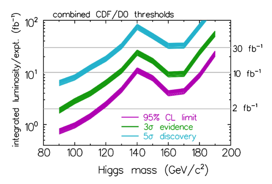
Figure 5.0.15: SUSY/Higgs Working Group estimations of the luminosity required for 95% exclusion, $3\sigma$ evidence, and $5\sigma$ discovery for the combined CDF+DØ search channels. (2000).

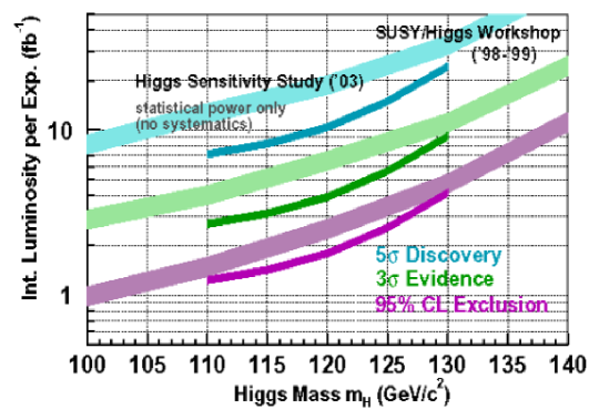
Figure 5.0.16: Higgs Sensitivity Working Group estimations of the luminosity required for 95% exclusion, $3\sigma$ evidence, and $5\sigma$ discovery for the combined CDF+DØ search channels, compared against the earlier SUSY/Higgs Working Group’s calculation.

The CDF channels as they stand as of the Summer 2005 conferences are not as powerful as those assumed in the two sensitivity studies. The following sections provide a snapshot of the sensitivity of the CDF channels separately and combined, as of the October 2005 TeV4LHC workshop, with plans for improvement.

Table 5.0.4: Integrated luminosities by channel.

Channel	$\int{\cal{L}}dt$ (pb-1)	Reference
$W^{\pm}H\rightarrow\ell^{\pm}\nu b{\bar{b}}$	319	[133]
$ZH\rightarrow\nu{\bar{\nu}}b{\bar{b}}$	289	[134]
$gg\rightarrow H\rightarrow W^{+}W^{-}$	360	[135]
$W^{\pm}H\rightarrow W^{\pm}W^{+}W^{-}$	194	[136]

5.1 Sensitivity by Channel

The expected signal and background rates and shape distributions were collected from each of the channel analysis teams and combined using the CL_s technique [137, 138] to find the expected limits on the cross-section multiplied by the branching fractions. Candidate information was not included in the combination, so the observed limit of the combination is not computed. All of the observed limits in the channels are close to expectations, the observed limit of the combination is expected to be close to the expected combined limit.

The $W^{\pm}H\rightarrow\ell^{\pm}\nu b{\bar{b}}$ Channel

The results of the $W^{\pm}H\rightarrow\ell^{\pm}\nu b{\bar{b}}$ search are described in [133]. The reconstructed mass distribution in the single-tagged analysis is used in computing the expected limits, with each bin counted as an independent counting experiment. Systematic errors are taken on the background and signal rates, but the shapes are not varied. Each bin is assumed to have fully correlated systematic uncertainties with all other bins of the mass distribution. The systematic uncertainties are detailed in Table 5.1.5. Acceptances and signal distributions are linearly interpolated [139] between the supplied test points at which Monte Carlo samples are available. The observed and expected cross-section times branching ratio limits are shown at the 95% CL in Figure 5.1.17 as a function of $m_{H}$.

Table 5.1.5: Relative systematic uncertainties by channel. Errors from the same source are considered correlated, across channels, and between signal and background. The “uncorrelated” errors are uncorrelated across channels and between signal and background.

	Channel
	$W^{\pm}H\rightarrow\ell^{\pm}\nu b{\bar{b}}$		$ZH\rightarrow\nu{\bar{\nu}}b{\bar{b}}$		$ZH\rightarrow\ell^{+}\ell^{-}b{\bar{b}}$		$gg\rightarrow H\rightarrow W^{+}W^{-}$		$W^{\pm}H\rightarrow W^{\pm}W^{+}W^{-}$
Source	s [% ]	b [% ]	s [% ]	b [% ]	s [% ]	b [% ]	s [% ]	b [% ]	s [% ]	b [% ]
lumi	6	6	6	6	6	6	6	6	6	6
b-tag s.f.	5		6.4	1.9	15	15			0.37
lepton ID	5				7	7
lepton trig	0.6				1	1			2.4
PDF	1								1.5
ISR	3								3.0
FSR	7				7				3.2
JES	3		7.8	3.5
Jet model	1.4
$\nu\nu b{\bar{b}}$ trig			3	1.5
$\nu\nu b{\bar{b}}$ veto			2	2
uncorrelated		15	2	22.1		9	6	7	3.7	66

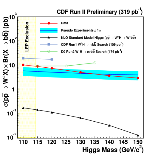
Figure 5.1.17: The observed and expected 95% CL limits on the production cross-section times the Higgs decay branching ratio as a function of $m_{H}$ for the $W^{\pm}H\rightarrow\ell^{\pm}\nu b{\bar{b}}$ channel. The limits are compared with the SM prediction.

The $ZH\rightarrow\nu{\bar{\nu}}b{\bar{b}}$ Channel

The results of the $ZH\rightarrow\nu{\bar{\nu}}b{\bar{b}}$ search are described in [134]. The reconstructed mass distribution was not provided for combination, but the numbers of events for the expected signal and background after a mass window cut which moves with the Higgs boson mass under test are used. They are linearly interpolated between the model points listed in [134]. The systematic uncertainties on the signal and background are detailed in Table 5.1.5. The observed and expected cross-section times branching ratio limit is shown at the 95% CL in Figure 5.1.18 as a function of $m_{H}$, and compared to the SM expectation.

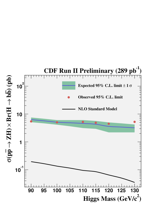
Figure 5.1.18: The observed and expected 95% CL limits on the production cross-section times the Higgs decay branching ratio as a function of $m_{H}$ for the $ZH\rightarrow\nu{\bar{\nu}}b{\bar{b}}$ channel. The liimts are compared with the SM prediction.

The $ZH\rightarrow\ell^{+}\ell^{-}b{\bar{b}}$ Channel

The $ZH\rightarrow\ell^{+}\ell^{-}b{\bar{b}}$ channel is still in development and the analysis is still in its “blind” stage. Hence, data candidate information is not yet available. The current status is described in [140]. The selection starts with a very clean sample of $Z\rightarrow\ell^{+}\ell^{-}$ decays, identifying isolated leptons with $m_{\ell\ell}$ close to $m_{Z}$, and two or three jets, at least one of which must be b-tagged. The systematic uncertainties on the signal and background are detailed in Table 5.1.5. The neural net has seventeen input variables described in [140]. The most powerful ones are the invariant mass of the two leading jets taken together, the event $H_{T}$ (which is the scalar sum of all the $P_{T}$’s of the observed particles), and the $E_{T}$ of the leading jet. The median expected limit on the cross-section times the branching ratio for this process is approximately 2.2 pb for 300 pb^-1 of data. This expected limit is lower than that for other channels mainly due to the very small background prediction. It must be compared, however, against a much smaller SM signal expectation.

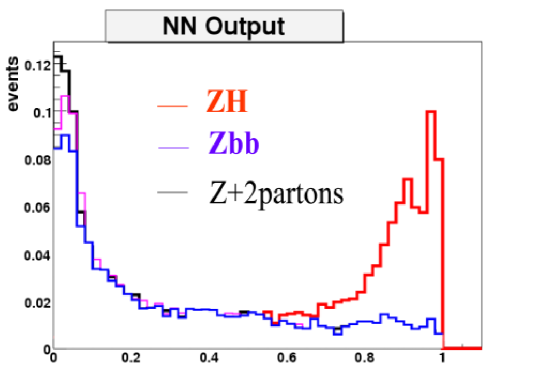
Figure 5.1.19: The distribution of the neural net discriminant function for the $ZH\rightarrow\ell^{+}\ell^{-}b{\bar{b}}$ channel, shown separately for the signal and for the major backgrounds, $Zb{\bar{b}}$ and $Z+2$ partons. The data in this channel are still blind.

The $gg\rightarrow H\rightarrow W^{+}W^{-}$ Channel

The results of the $gg\rightarrow H\rightarrow W^{+}W^{-}$ search are described in [135]. The histograms of $\Delta\phi_{\ell\ell}$ are used as the discriminant variable input to the limit calculation – each bin is a separate counting experiment. The shapes are interpolated [139] between $m_{H}$ points, as are the signal rates and background rates. The analysis uses $m_{H}$-dependent cuts, and so the background rates depend on the $m_{H}$ under test. The systematic uncertainties on the signal and background are detailed in Table 5.1.5.

The median expected 95% CL cross-section times branching ratio limit is shown in Figure 5.1.20 as a function of $m_{H}$ compared to the SM expectation and to the computation of [135].

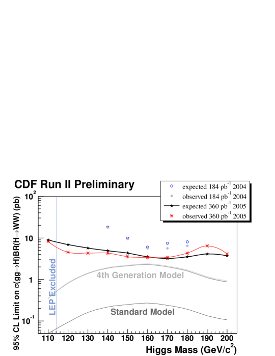
Figure 5.1.20: The observed and expected 95% CL limits on the production cross-section times the Higgs decay branching ratio as a function of $m_{H}$ for the $gg\rightarrow H\rightarrow W^{+}W^{-}$ channel. The limits are compared with the SM prediction, and also the prediction of a model with a heavy fourth generation of SM-like fermions.

The $W^{\pm}H\rightarrow W^{\pm}W^{+}W^{-}$ Channel

The results of the $W^{\pm}H\rightarrow W^{\pm}W^{+}W^{-}$ search are described in [136]. It is a single counting experiment – there are no discriminant variables whose histograms have different $s/b$ ratios to use. The acceptance is interpolated between the $m_{H}$ points listed in [136]. The systematic uncertainties on the signal and background are detailed in Table 5.1.5. For this calculation, the data statistical uncertainty on the residual conversion background is treated as independent of the other errors on the background and the errors add in quadrature instead of linearly as they do in [136]. Furthermore, the FSR systematic uncertainty is almost certainly truly uncorrelated with other channels’ FSR uncertainty, but it has been treated as correlated. As is seen below, the entire systematic error treatment in this channel matters little to the sensitivity.

The observed cross-section times branching ratio limit is shown at the 95% CL in Figure 5.1.21 as a function of $m_{H}$ compared to the SM expectation and to the computation of [136].

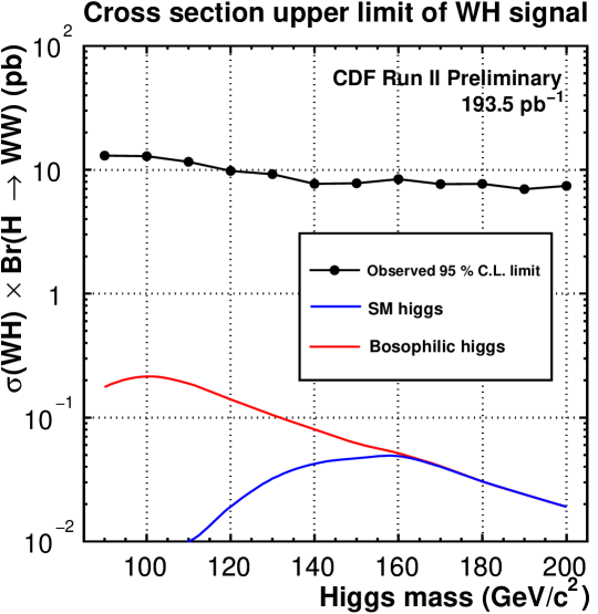
Figure 5.1.21: The observed 95% CL limit on the production cross-section times the Higgs decay branching ratio as a function of $m_{H}$ for the $W^{\pm}H\rightarrow W^{\pm}W^{+}W^{-}$ channel. The limits are compared with the SM prediction, and also the prediction of a “bosophilic” (also known as “fermiophobic”) model.

5.2 Sensitivity of the SM Channels when Combined

The observed 95% CL limits in all of CDF’s SM Higgs channels are shown, compared with SM predictions, and also compared with observed limits from DØ’s channels, in Figure 5.2.22. The different searches search for different processes which have different rates, and thus contribute differently to the combined sensitivity. It is somewhat easier to compare the channels’ sensitivity to a SM Higgs when the ratio of the limit in each channel to the SM prediction is formed. This ratio is shown for the same collection of CDF and DØ channels in Figure 5.2.23.

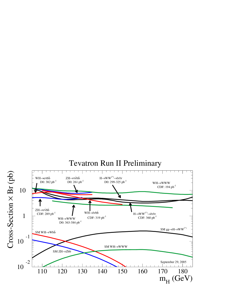
Figure 5.2.22: The observed 95% CL limits on the production cross section times the Higgs decay branching ratio for each of the five search channels, compared with DØ’s limits, and also compared with SM expectations.

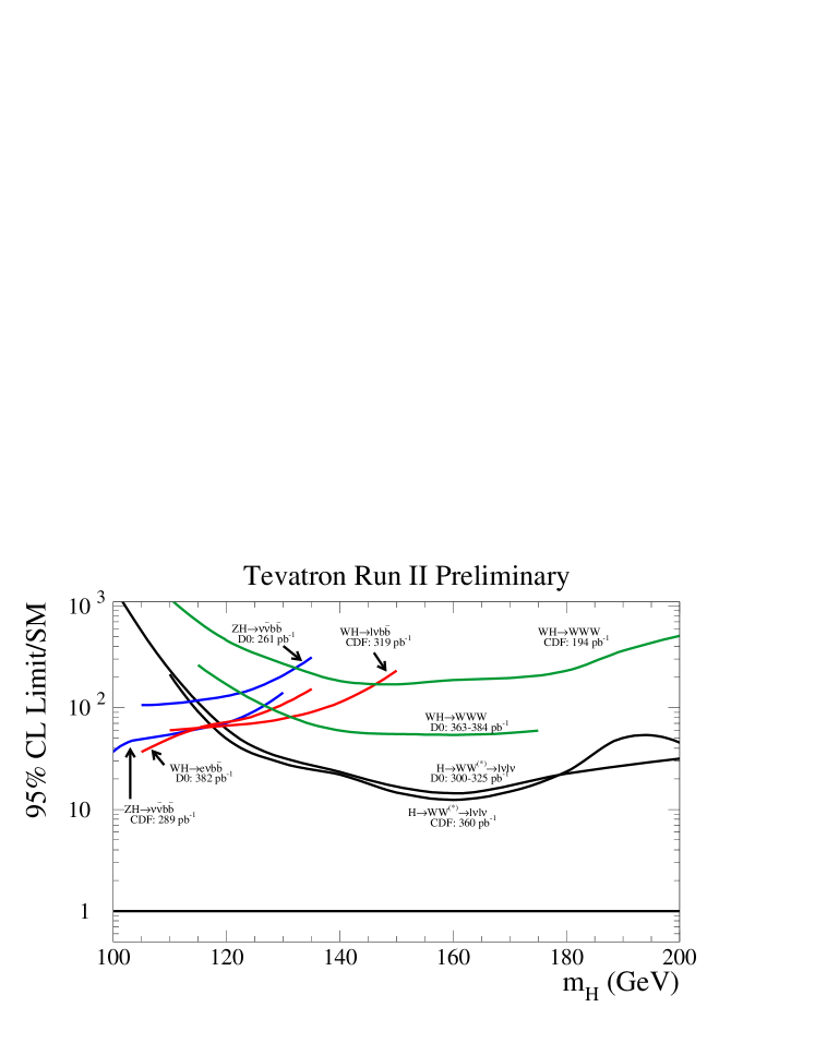
Figure 5.2.23: CDF and DØ’s observed 95% CL limits on the production cross section times the Higgs decay branching ratio, divided by the corresponding SM predictions, for each of the five search channels.

The CL_s method is used on the collection of CDF’s five SM Higgs boson search channels to compute the multiplicative scale factor $s_{95}$ on the total signal which can just barely be expected to be excluded in a median experimental outcome. This procedure doesn’t make much physical sense for scale factors exceeding unity, as there isn’t a well-motivated physical model which scales all of the production mechanisms for SM Higgs bosons in the same way, but it provides a technical benchmark of how far we are from the SM in our sensitivity. The results of this combination are shown in Figure 5.2.24. It must be shown as a multiplicative factor of the SM prediction because of the different SM predictions used for each search channel.

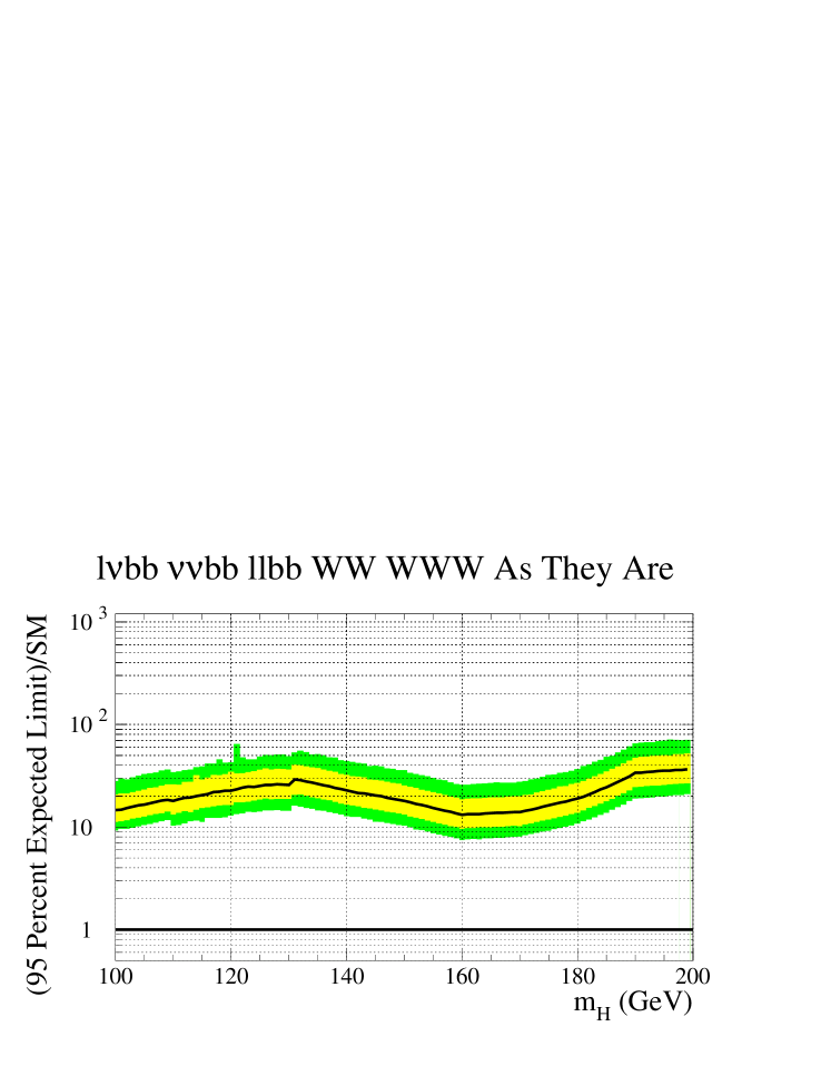
Figure 5.2.24: The expected 95% CL limit on the multiplicative scale factor of SM Higgs boson production for CDF’s five SM Higgs boson search channels combined, as a function of $m_{H}$, assuming the absence of a Higgs boson. The yellow and green bands show the $\pm 1\sigma$ and $\pm 2\sigma$ expectations, which fluctuate depending on the possible data which may be observed.

5.3 Necessary SM Channel Improvements

The current channels as we have them are insufficient to test for the presence or absence of the Standard Model Higgs boson, even if the projected 8 fb^-1 of data are collected. Improvements must be made to increase the acceptance, reduce the background, and to separate the selected events into disjoint subsets with different $s/b$ ratios, and to combine them together. Furthermore, the results must be combined with DØ.

The Higgs Sensitivity Working Group report [132] lists changes which can be made to the analyses which can get us to the desired level of sensitivity. Much of this work has already been done to improve our resolutions, to increase our lepton acceptance to the forward region, and to develop neural nets. But the work has been done by a variety of different people separated in space, time, and institution. The work of many groups must be collected together in the analysis channels in order to achieve the sensitivity reported in [4, 132].

The factors on the expected amount of luminosity needed to get exclusion at the 95% CL, $3\sigma$ evidence and $5\sigma$ discovery can be computed for most of the improvements rather easily. For acceptance increases, the background ought to increase as the signal acceptance increases. In fact, it should increase faster, because as we expand our acceptance to forward regions of the detector or to include leptons of lower quality, a larger fraction of background is expected to creep in. For this estimation, the estimations are taken from the HSWG report’s Sections 2.3 and 4.2 (for the Neural Net factor). A listing of improvements and their factors in luminosity is given in Table 5.3.6. It is assumed in the luminosity projections that the systematic uncertainties will scale inversely with the square root of the integrate luminosity. Furthermore, accounting of the shape uncertainties may make the systematic errors larger.

Table 5.3.6: Luminosity factors expected from analysis improvements, separated by channel.

Improvement	$W^{\pm}H\rightarrow\ell^{\pm}\nu b{\bar{b}}$	$ZH\rightarrow\nu{\bar{\nu}}b{\bar{b}}$	$ZH\rightarrow\ell^{+}\ell^{-}b{\bar{b}}$
$m_{H}$ Resolution	1.7	1.7	1.7
Continuous b-tags	1.5	1.5	1.5
Forward B-tags	1.1	1.1	1.1
Forward Leptons	1.3	1.0	1.6
Neural Nets	1.75	1.75	1.0
Track-Only Leptons	1.4	1.0	1.6
WH signal in ZH	1.0	2.7	1.0
Product of above	8.9	13.3	7.2
CDF+DØ Combination	2.0	2.0	2.0
All Combined	17.8	26.6	14.4

The neural net factor of 1.75 is not uniformly applicable to all channels, as the $ZH\rightarrow\ell^{+}\ell^{-}b{\bar{b}}$ channel estimations already take advantage of a neural net. The forward lepton acceptance improvement cannot strictly be multiplied by the track-only lepton factor since the forward tracking is not sufficient. Nonetheless, a naive product of the factors from the analysis improvements is approximatley 20. The analysis improvements will not be made all at once – work is ongoing to develop and characterize the techniques.

5.4 SM Sensitivity Projections

Assuming that the acceptances of the channels are increased and neural nets or other advanced techniques are used to reduce the backgrounds, the projected reach of of the Tevatron SM Higgs search program is estimated. It is assumed that the systematic uncertainties scale inversely with the square root of the integrated luminosity, and that DØ contributes channels with the same sensitivity as CDF’s and that they are combined together. Figure 5.4.25 shows how the significance of an excess of events is expected to develop, as a function of the integrated luminosity collected per experiment, assuming a SM Higgs boson is present with a mass $m_{H}=115$ GeV. The actual evolution of such an excess, if a signal is actually present, will be more of a random walk as data are collected, so the figure also includes the width of the expected distribution. Figure 5.4.26 shows the evolution of the probability of seeing a $2\sigma$, a $3\sigma$, or a $5\sigma$ excess in the combined data when searching for a SM Higgs boson of mass $m_{H}=115$ GeV, if it is truly present, as a function of the luminosity collected by each experiment. After collecting 8 fb^-1 per experiment, it is 10% likely that a $5\sigma$ excess will be observed if $m_{H}$ is truly 115 GeV.

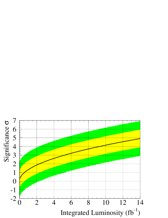
Figure 5.4.25: The evolution of the expected significance of an excess in the data if a Standard Model Higgs boson is present with a mass of 115 GeV. The yellow (light) interior band shows the $\pm 1\sigma$ distribution of the expected significance, and the green (darker) exterior band shows the $\pm 2\sigma$ range around the expectation. CDF and DØ are combined, and the foreseen sensitivity improvements have been assumed. The integrated luminosity is per experiment.

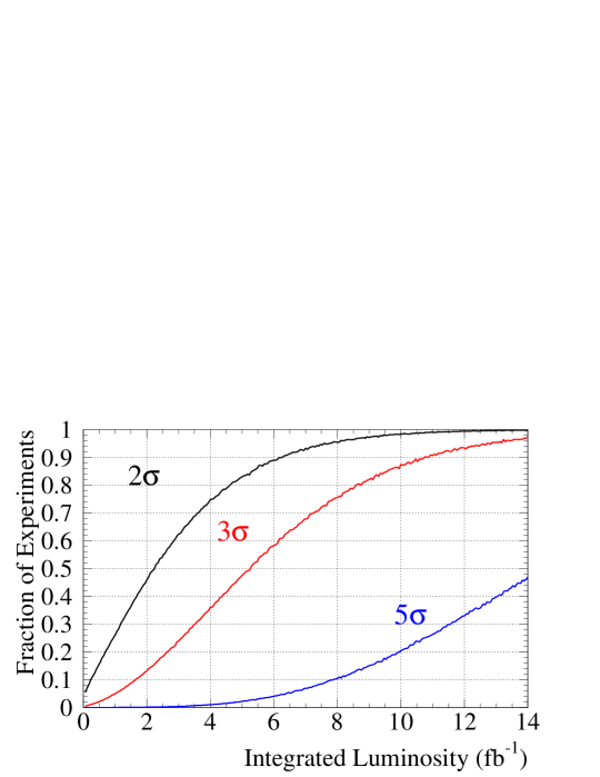
Figure 5.4.26: The fraction of experiments expected to make an observation of a 115 GeV SM Higgs boson if it is truly there, as a function of the integrated luminosity. CDF and DØ are combined, and the foreseen sensitivity improvements have been assumed. Separate curves are shown for the fraction of experiments observing a $\geq 2\sigma$ excess in the data, a $\geq 3\sigma$ excess, or a $\geq 5\sigma$ excess.

5.5 The MSSM $H/h/A\rightarrow\tau^{+}\tau^{-}$ Sensitivity

CDF has published its search for $H/h/A\rightarrow\tau^{+}\tau^{-}$ search, using 310 pb^-1 of Run 2 collision data [89]. Tau pairs are selected in which one tau decays leptonically, and the other decays semi-hadronically. Kinematic selection requirements were designed to separate tau pairs from $W$+jets and QCD backgrounds, in which jets are misidentified as taus. The dominant remaining background is $Z\rightarrow\tau^{+}\tau^{-}$ production. In order to separate $H/h/A\rightarrow\tau^{+}\tau^{-}$ from this and other backgrounds, the invariant mass of the visible tau decay products is formed, shown in Figure 5.5.27. The reconstructed invariant mass of Higgs boson signal events peaks near the signal mass, with a width which grows rapidly with increasing Higgs boson signal mass. This is offset by the fact that the background is very small for large reconstructed masses. The observed and expected limits on the production cross section times the decay branching ratio to tau pairs is shown in Figure 5.5.28.

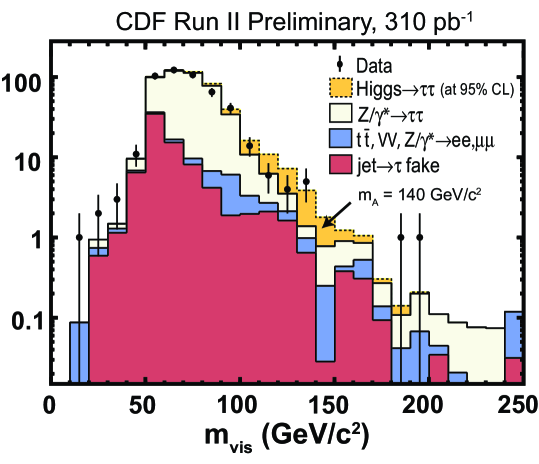
Figure 5.5.27: The invariant mass of the reconstructed tau decay products in the MSSM $H\rightarrow\tau^{+}\tau^{-}$ search. The data (points) are compared to a sum of background predictions. A Higgs boson signal of mass $m_{A}=140$ GeV, with a production cross section just at the exclusion threshold, is shown.

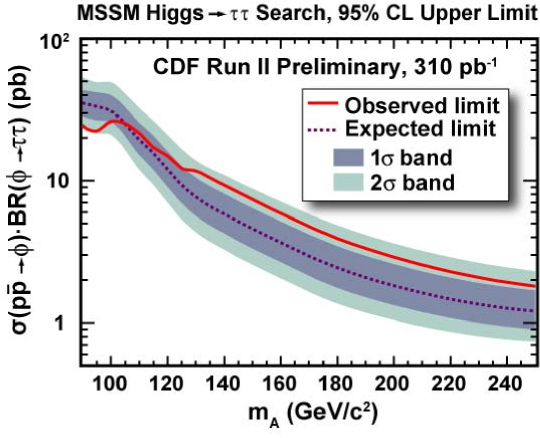
Figure 5.5.28: The 95% CL limit on the production cross section times the decay branching ratio for Higgs bosons decaying to tau pairs, using 310 pb^-1 of CDF data, as a function of the Higgs boson mass.

This cross-section limit can be interpreted in the MSSM; we choose to represent it as an exclusion in the $(m_{A},\tan\beta)$ plane in the $mh-max$ and $no-mixing$ MSSM benchmark scenarios [141]. This interpretation benefits from the fact that for larte $\tan\beta$, two Higgs bosons (either $h$ and $A$, or $H$ and $A$), are nearly degenerate in mass and contribute rougly equally to the expected signal. CDF’s observed 95% CL limits are shown in Figure 5.5.29, along with projected CDF+DØ combined sensitivity contours for 2, 4, and 8 fb^-1 of data collected by both CDF and DØ. The large improvement in sensitivity at larger Higgs boson masses comes from the fact that the background rate is very low for large invariant-mass tau pairs. For a search with a large background rate, the expected signal limit is roughly inversely proportional to the square root of the integrated luminosity, while for searches with very small backgrounds, the expected limit is roughly inversely proportional to the integrated luminosity.

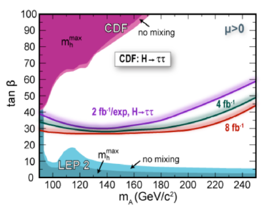
Figure 5.5.29: The observed 95% CL limits in the tau channel in the $(m_{A},\tan\beta)$ plane, for the $m_{H}$-max MSSM benchmark scenerio and also the no-mixing benchmark scenario, using 310 pb^-1 of CDF data. Projections are shown for the expected combined CDF+DØ exclusion reach for 2, 4, and 8 fb^-1 per experiment.

6 Two-Loop EW Corrections to Higgs Production

Contributed by: U. Aglietti, R. Bonciani, G. Degrassi, A. Vicini

We study the impact of the two-loop electroweak corrections on the production of a Higgs boson via gluon-fusion in proton-proton collisions at LHC energies. We discuss the prescritpion to include the corrections to the hard scattering matrix element in the calculation of the hadronic cross-section $\sigma(p+p\to H+X)$. Under the hypothesis of factorization of the electroweak corrections with respect to the dominant soft and collinear QCD radiation, we observe an increase of the total cross-section from 4 to 8%, for $m_{h}\leq 160~{}{\rm GeV}$. This increase is comparable with the present QCD uncertainties originating from hard scattering matrix elements.

6.1 Introduction

We study the impact of the two-loop electroweak corrections on the production of a Higgs boson via gluon-fusion in proton-proton collisions at LHC energies. We discuss the prescritpion to include the corrections to the hard scattering matrix element in the calculation of the hadronic cross-section $\sigma(p+p\to H+X)$. Under the hypothesis of factorization of the electroweak corrections with respect to the dominant soft and collinear QCD radiation, we observe an increase of the total cross-section from 4 to 8%, for $m_{h}\leq 160~{}{\rm GeV}$. This increase is comparable with the present QCD uncertainties originating from hard scattering matrix elements.

The Higgs boson is one of the missing ingredients of the Standard Model and its discovery represents one of the most important physics goals of the LHC. This goal will be achieved only if we can predict with high accuracy all the production cross sections of this particle and if we understand in detail the different decay channels and the relative backgrounds.

At the LHC, the gluon-fusion is the dominant production mode over the entire range of interesting values of the mass of the Higgs particle ($100\mathrm{\ Ge\kern-1.00006ptV}\lesssim m_{H}\lesssim 1\mathrm{\ Te\kern-1.00006ptV}$). In particular, in the range $100\mathrm{\ Ge\kern-1.00006ptV}\lesssim m_{H}\lesssim 2m_{t}$ this production mode is larger by almost one order of magnitude with respect to the next important mechanism, the vector boson fusion. It is, therefore, very important to have a precise prediction of its cross section and a reliable estimate on the remaining theoretical accuracy.

The total cross section for the Higgs boson production by gluon fusion in the LO approximation was calculated in the late seventies [142]. It is an ${\mathcal{O}}(\alpha_{S}^{2}\,\alpha)$ calculation, since the Higgs couples to the gluons only via an heavy-quark loop (the most important contribution is the one due to the loop of top). For what concerns the higher orders, the calculation of the NLO QCD corrections have been done in the infinite $m_{t}$ (mass of the top) limit in [143], and, with the full quark mass dependence, in [20]. Besides of the fact that the infinite $m_{t}$ approximation should be valid in the Higgs mass range $m_{H}\lesssim 300$ GeV, it has been noticed [144] that this approximation works also for values of $m_{H}$ beyond the top threshold, and up to masses of ${\mathcal{O}}(1\mathrm{\ Te\kern-1.00006ptV})$. The total effect of the NLO QCD corrections is the increase of the LO cross section by a factor 1.5–1.7, giving a residual renormalization/factorization scale dependence of about 30%. The unexpected size of the NLO QCD radiative corrections made in such a way that the electroweak corrections, evaluated in the infinite $m_{t}$ limit in [145, 146] and turning out to amount of less that 1%, were totally neglected. The attention was driven by the evaluation of the NNLO QCD corrections, carried out in the infinite $m_{t}$ limit by several groups [147, 148, 149, 150, 151, 152]. The calculation shows a good convergence of the perturbative series: while the NNLO corrections are sizable, they are, nevertheless, smaller that the NLO ones. Moreover, the NNLO corrections improve the stability agaist renormalization/factorization scale variations. The effect due to the resummation of soft-gluon radiation has been included in [153], and the remaining theoretical uncertainty, due to higher-order QCD corrections, has been estimated to be smaller than 10%. Finally, several efforts were also devoted to the calculation of QCD radiative corrections to less inclusive quantities, such as the rapidity distribution, recently evaluated at the NNLO [154, 155], or the transverse momentum ($q_{T}$) distribution [156, 157, 158, 159, 160, 161, 162, 163, 164, 165, 166, 167, 168, 169, 170, 171, 172, 173, 174, 175, 176, 177, 178], which, in [179, 180], is evaluated using the fixed-order perturbative results up to NLO in QCD and the resummation up to the NNLL.

Motivated by this accurate scenario, the NLO electroweak corrections to the gluon fusion were again taken into account recently. In [181, 182] the contribution to the partonic cross section due to the light fermions were calculated. It turned out that they are sizeable. In particular, in the intermediate Higgs mass range, from 114 GeV up the the $2m_{W}$ threshold, these corrections increase the LO partonic cross section by an amount of 4–9%. For larger values of the mass of the Higgs, $m_{H}>2m_{W}$, they change sign and reduce the LO cross section; however, in this region the light-fermion corrections are quite small, reaching at most a -2%. In [183], also the remaining electroweak corrections due to the top quark were calculated as a Taylor expansion in $m_{H}^{2}/(4m_{W}^{2})$. They are valid for $m_{H}\lesssim 2m_{W}$, range in which they have opposite sign with respect to the light-fermion corrections. However, the corrections due to the top quark are smaller in size, reaching at most a 15% of the light-quark ones.

The impact of the NLO electroweak corrections on the hadronic cross section has not been discussed yet. We present here the effect of their inclusion in the calculation at the hadronic level.

6.2 Inclusion of the Two-Loop Electroweak Corrections

The partonic gluon fusion process occurs, in lowest order, via one-loop diagrams, as the one depicted in Fig. 6.2.30 (a);

Figure 6.2.30: Lowest order (a) and generic NLO-EW (b), (c), (d) Feynman diagrams. The solid lines are fermions. The wavy lines are gauge bosons $(V=W,Z)$.

in the loop run only the top and the bottom quarks, because of the Yukawa suppression of the lighter quarks. The NLO-EW corrections are schematically represented by the diagrams in Figs. 6.2.30 (b), (c) and (d). In particular, in Figs. 6.2.30 (b) and (c) the WWH/ZZH couplings avoid the Yukawa suppression, and, therefore, in these diagrams the fermionic line represents all the possible flavours: light flavours, evaluated in [181, 182], and top quark, evaluated in [183]. In Fig. 6.2.30 (d), instead, the fermionic line can represent only the top quark [183].

At the hadronic level, we consider the Higgs boson production at the LHC, and therefore in proton-proton collisions. The hadronic cross section can be written as:

$$\sigma(p+p\to H+X)=\sum_{a,b}\int_{0}^{1}dx_{1}dx_{2}\,\,f_{a,p}(x_{1},M^{2})\,f_{b,p}(x_{2},M^{2})\times$$

$$~{}~{}~{}~{}~{}~{}~{}~{}~{}~{}~{}~{}~{}~{}~{}~{}~{}~{}~{}~{}~{}~{}~{}~{}~{}~{}~{}\times\int_{0}^{1}dz~{}\delta\left(z-\frac{\tau_{H}}{x_{1}x_{2}}\right)~{}\Big{(}1+\delta_{EW}(m_{h})\Big{)}\hat{\sigma}_{ab}(z)$$

$$\hat{\sigma}_{ab}(z)=\hat{\sigma}_{0}\,\left(1+K^{QCD~{}only}_{ab}(\alpha_{s}(\mu^{2}),\mu^{2},M^{2})\right)$$ (6.2.57)

where the partonic processes initiated by partons $(a,b)$ are convoluted with the corresponding parton densities $f_{i,p}(x,M^{2}),~{}~{}(i=a,b)$, evaluated at a scale $M$. The effect of the higher order QCD and EW corrections is described by the two functions $K^{QCD-only}$ and $\delta_{EW}$, obtained by factoring the lowest order cross section $\hat{\sigma}_{0}$.

In the partonic cross section, QCD and EW corrections have been factorized. This ansatz is valid up to subleading higher order corrections which start at the 3-loop level (i.e. ${\cal O}(\alpha\alpha_{s})$ with respect to the lowest order). The factorization of the QCD initial state collinear divergences holds for the hard process described by the electroweak NLO corrections, following from general arguments of the factorization theorems and from the universal nature of the initial state collinear radiation. In fact, the whole set of EW corrections is characterized by a scale $\mbox{M}_{\mbox{W}}$, much harder than the one typical of the leading collinear emission. In addition, in the limit of light Higgs, the EW corrections can be expanded as a Taylor series in powers of $m_{h}/\mbox{M}_{\mbox{W}}$ and the EW corrections vertex becomes effectively pointlike. In this regime the factorization of the QCD collinear divergences becomes rigorous. For heavier Higgs masses, the factorization should still be valid only in leading order, due to the modifications induced by the EW form factor.

6.3 Numerical Results

The hadronic proton-proton cross section has been calculated at LHC energy, in NNLO-QCD accuracy, i.e. setting $\delta_{EW}=0$, using the MRST2002 NNLO parton distribution functions [184]. The theoretical uncertainty due to the choice of the renormalization scale $\mu$ and of the factorization scale $M$ has been canonically estimated by setting $M=\mu$ equal to $m_{h}/2,m_{h},2m_{h}$ respectively. The predictions, shown in Fig. 6.3.31 (dotted lines), vary by approximately $\pm 8$% with respect to the central value. This uncertainty is further reduced when including the effect of the resummation of all the initial state soft gluon radiation [153].

Figure 6.3.31: The cross section $\sigma_{p+p\to H+X}$, in pb, is plotted as a function of the mass of the Higgs boson, between 114 GeV and 300 GeV. The dotted lines describe the band of NNLO-QCD uncertainty, for three values of the QCD factorization/renormalization scale $\mu=m_{h}/2,m_{H},2m_{h}$. The solid line is the NNLO-QCD $(\mu=m_{h})$ with the two-loop EW corrections, according to Eq. (6.2.57). The two-loop EW corrections include also the top-quark effect, for $m_{h}\leq 155$GeV, but only the light quarks contribution for larger values of $m_{h}$.

The two-loop electroweak corrections have been added according to Eq. (6.2.57) and setting $M=\mu=m_{h}$. The light fermion corrections can be evaluated for any choice of $m_{h}$, whereas the top quark contribution has been computed by means of a Taylor expansion and is limited to the region $m_{h}\leq 160$GeV. The hadronic cross section increases from 4 to 8%, for $m_{h}\leq 160$ GeV. As we can observe in Fig. 6.3.31, the effect of the electroweak corrections is an increase of the cross section by an amount which is of the same order of magnitude of the NNLO-QCD theoretical uncertainty, and possibly larger than the uncertainty estimated after the resummation of soft gluon radiation. The main source of uncertainty on the hadronic cross section remains in the accurate determination of the parton distribution functions of the proton.

The effect of the NLO-EW corrections is of great interest, because it enhances the most important Higgs production mechanism and, in turn, affects the absolute number of events of all the Higgs decay modes.

Following Eq. (6.2.57), the NLO-EW corrections can be implemented as a simple rescaling of the QCD hadronic cross section. This multiplicative factor is presented in Table 6.3.7 as a function of $m_{h}$ and can be fitted, in the range $114\mathrm{\ Ge\kern-1.00006ptV}\lesssim m_{H}\lesssim 155\mathrm{\ Ge\kern-1.00006ptV}$, by the following simple formula:

$$\delta_{EW}(m_{H})=1.00961+6.9904\cdot 10^{-5}\,m_{h}+2.31508\cdot 10^{-6}\,m_{h}^{2}\,.$$ (6.3.58)

$m_{h}$ (GeV)	$\delta_{EW}$	$m_{h}$ (GeV)	$\delta_{EW}$	$m_{h}$ (GeV)	$\delta_{EW}$	$m_{h}$ (GeV)	$\delta_{EW}$
114	1.048	136	1.062	158	1.077	180	1.020
116	1.049	138	1.063	160	1.069	182	1.010
118	1.050	140	1.065	162	1.063	184	1.010
120	1.051	142	1.066	164	1.049	186	1.002
122	1.053	144	1.068	166	1.041	188	0.997
124	1.054	146	1.069	168	1.035	190	0.994
126	1.055	148	1.071	170	1.031	192	0.991
128	1.056	150	1.073	172	1.028	194	0.989
130	1.058	152	1.074	174	1.026	196	0.987
132	1.059	154	1.076	176	1.024	198	0.986
134	1.060	156	1.077	178	1.022	200	0.985

Table 6.3.7: Rescaling factor $\delta_{EW}$ as a function of the Higgs boson mass.

The computation of the NLO-EW corrections to the gluon fusion process has been described in detail in [181, 182, 183]. The analytical expression of the probability amplitude has been expressed in terms of Generalized Harmonic PolyLogarithms (GHPL) [185] and has been implemented in a FORTRAN routine. The GHPL can be evaluated numerically in several different ways: by direct numerical integration of the basic functions, by power expansions or by solving the associated differential equations. We have checked that these fully independent approaches agree.

6.4 Conclusions

In conclusion, the calculation of the QCD corrections to the production of a Higgs boson via gluon-fusion has reached a very high level of accuracy; it is now mandatory the inclusion of the two-loop electroweak corrections, whose typical size for $m_{h}\leq 160$ GeV is larger than 5%, comparable or larger than the QCD uncertainty. The main source of uncertainty on the hadronic cross section remains in the accurate determination of the parton distribution functions of the proton.

Acknowledgments

The authors wish to thank S. Catani, D. de Florian and M. Grazzini for allowing the use of the numerical program of JHEP 0105 (2001) 025 [arXiv:hep-ph/0102227], and for useful discussions.

This work was partly supported by the European Union under the contract HPRN-CT2002-00311 (EURIDICE) and by MCYT (Spain) under Grant FPA2004-00996, by Generalitat Valenciana (Grants GRUPOS03/013 and GV05/015).

7 Higgs Resummation

Contributed by: B.J. Field

Resummation when combined with fixed-order calculations yield the most accurate theoretical definition for differential cross-sections for use by the experimental community to correctly determine and unambiguously reconstruct the mass of any Higgs bosons that may exist in nature. There has been excellent progress in recent years at obtaining higher-order fixed-order results for all the relevant Higgs production processes. It is therefore necessary to follow these calculations with resummed calculations to complete our theoretical understanding ahead of future collider data.

Resummation of processes involving both scalar and pseudoscalar Higgs bosons have been studied extensively[186, 187, 188, 189, 190, 144, 191, 192, 193, 194, 195, 196, 197, 23, 198, 199, 200, 201, 202]. In order to understand the small-$p_{T}$ behavior of a differential cross-section, we need to employ the resummation formalism[203, 204, 205]. Resummation will smooth out any numeric instabilities and divergencies that occur in fixed order calculations.

There are several ways to approach resummation of both total cross-sections and differential quantities. Here we will discuss only the differential quantities as they are more relevant for experimental concerns. The formalism of resummation is different depending on what kind of observable one is interested in studying. Although much of the work of resummation has focused on inclusive production, it is possible to study exclusive processes[206].

For inclusive processes where typically only one particle is produced at lowest order, the standard formalism allows a resummed differential cross-section to be written as an inverse Bessel transformation in terms of an expansion in $\alpha_{s}$ of both universal and process-dependent terms. For instance,

$$\frac{d\sigma^{\textrm{resum}}}{dp_{t}^{2}\,dy\,d\phi}=\sum_{a,b}\int_{x_{1,\textrm{min}}}^{1}\!\!\!dx_{1}\int_{x_{2,\textrm{min}}}^{1}\!\!\!dx_{2}\int_{0}^{\infty}db\,\frac{b}{2}J_{0}(bp_{t})$$

$$\times f_{a/h_{1}}\!(x_{1},b_{0}/b)\,f_{b/h_{2}}\!(x_{2},b_{0}/b)\,\frac{S}{Q^{2}}W_{ab}(x_{1}x_{2}S;Q,b,\phi),$$

where we define,

$$W_{ab}(s;Q,b,\phi)=\sum_{c}\int_{0}^{1}dz_{1}\int_{0}^{1}dz_{2}\,\bar{C}_{ca}(\alpha_{s}(b_{0}/b),z_{1})$$

$$\times\bar{C}_{\bar{c}b}(\alpha_{s}(b_{0}/b),z_{2})\,\delta(Q^{2}-z_{1}z_{2}s)\,\frac{d\sigma_{\bar{c}c}^{LO}}{d\phi}\,S_{c}(Q,b),$$

and the Higgs mass is $M_{\Phi}^{2}=Q^{2}$, $d\phi$ is any unintegrated phase space of the system under consideration, and $\hat{\sigma}^{(LO)}_{c\bar{c}}$ is the lowest order cross-section with a $c\bar{c}$ initial state which is therefore defined at $p_{t}=0$. Since this is an inclusive process, the transverse momentum and rapidity in the differential cross-section $(p_{t},y)$ are that of the Higgs boson produced. The integration variable $b$ is the impact parameter, $S$ is the center-of-momentum energy of the hadronic system, and the $f_{i/A}$ are the parton distribution functions for a parton $i$ in hadron $A$. The constant $b_{0}$ is written in terms of the Euler-Mascheroni constant $\gamma_{E}=0.57721\ldots$ as $b_{0}=2e^{-\gamma_{E}}$ to simplify the coming coefficient expressions. The coefficients $C_{ab}$ are process dependent and can be written as power series to be described below. $J_{0}(bp_{t})$ is the first order Bessel function. The Sudakov form factor $S_{c}$, which makes the integration over the Bessel function convergent, can be written as,

$$S_{c}(Q,b)=\exp\biggl{\{}-\int^{Q^{2}}_{b_{0}^{2}/b^{2}}\frac{dq^{2}}{q^{2}}\biggl{[}A_{c}(\alpha_{s}(q))\ln\frac{Q^{2}}{q^{2}}+B_{c}(\alpha_{s}(q))\biggr{]}\biggr{\}}.$$ (7.0.59)

The coefficient functions $A_{c}$, $B_{c}$, and $C_{ab}$ can be written as power series in $\alpha_{s}$ as

$$A_{c}(\alpha_{s})=\sum_{n=1}^{\infty}\biggl{(}\frac{\alpha_{s}}{\pi}\biggr{)}^{n}A_{c}^{(n)},\quad B_{c}(\alpha_{s})=\sum_{n=1}^{\infty}\biggl{(}\frac{\alpha_{s}}{\pi}\biggr{)}^{n}B_{c}^{(n)},$$ (7.0.60)

$$\bar{C}_{ab}(\alpha_{s},z)=\delta_{ab}\delta(1-z)+\sum_{n=1}^{\infty}\biggl{(}\frac{\alpha_{s}}{\pi}\biggr{)}^{n}\bar{C}_{ab}^{(n)}(z).$$ (7.0.61)

The $A^{(1)}_{c}$, $A^{(2)}_{c}$, and $B^{(1)}_{c}$ coefficients have been shown to be universal.

Although this particular method of handling resummed differential cross-sections is useful, it ignores several of the more interesting channels where a Higgs boson would be produced in association with another particle, and therefore has nothing to say about the other particles in the process. There has been interest in a Higgs bosons produced in association with weak vector bosons, light and heavy quarks, and combinations of these particles as can easily be seen in the cross-sections that have been compiled for this workshop. In particular, there is continuing theoretical[41, 207, 38, 37, 208, 39, 209, 40] and experimental[88] interest in a Higgs produced in association with bottom quarks, particularly in supersymmetric models where bottom quarks can play a role equal to or greater than top quarks in Higgs processes.

To understand resummed processes for a more general particle configuration can be calculated with a different mechanism[206] which can be used for inclusive, exclusive, and the resummation of pair-invariant-mass quantities. This formalism is setup as a unified approach that allows one to perform the resummation based on the color flow of the chosen process as well as several previously calculated quantities.

If we define a generic plus-distribution related object in terms of the variable that becomes soft $(s_{4})$ or zero $(1-z)$ on threshold as

$$\mathcal{D}_{l}(s_{4})\equiv\biggl{[}\frac{\ln^{l}(s_{4}/M^{2})}{s_{4}}\biggr{]}_{+},\qquad\textrm{or},\qquad\mathcal{D}_{l}(z)\equiv\biggl{[}\frac{\ln^{l}(1-z)}{1-z}\biggr{]}_{+},$$ (7.0.62)

then at next-to-leading-log (NLL) accuracy we can define a total or differential cross-section, where we generically call the threshold variable $x_{\textrm{th}}$, as

$$d\hat{\sigma}=d\sigma^{\textrm{B}}\frac{\alpha_{s}}{\pi}\biggl{\{}c_{3}\mathcal{D}_{1}(x_{\textrm{th}})+c_{2}\mathcal{D}_{0}(x_{\textrm{th}})+c_{1}\delta(x_{\textrm{th}})\biggr{\}},$$ (7.0.63)

where $d\hat{\sigma}$ can be either a total or differential quantity of interest and $d\sigma^{\textrm{B}}$ is the total or differential Born cross-section. There exists a similar equation of the NNLL corrections that will not be reproduced here but can be found in the literature[206]. The coefficients $c_{i}$ can be calculated in terms of the color Casimir invariants of the partons involved in the process, the soft anomalous dimension matrix, and the kinematic invariants of the process. At higher orders, the expressions become more complicated, but straightforward to calculate in a unified manner for several different processes.

The results of the Higgs calculations in the literature tells us several qualitative facts about resummed Higgs processes. First, the resummed quantities are finite at small-$p_{T}$ and removed the fixed-order divergencies. We also find smaller scale uncertainties at higher-orders as expected.

The two primary inclusive Higgs processes that have been studied are $gg\rightarrow\Phi$ and $b\bar{b}\rightarrow\Phi$, where $\Phi$ is generically any Higgs boson of interest. Some sample resummation calculation for inclusive Higgs from Refs [199, 200] are shown in Figure 7.0.32.

Aside from the usual observations for these differential cross-sections, we can see that the total uncertainty in the magnitude of the cross-section at the peak, from parton distribution functions and a scale variation by a factor of two, is approximately $35$%. This level of theoretical uncertainty is on par with similar fixed order calculations.

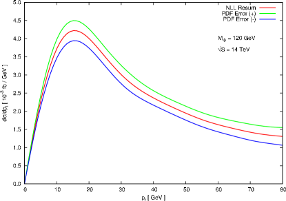
(a)	(b)

Figure 7.0.32: Figure 7.0.32a shows the transverse momentum spectrum for a scalar Higgs boson produced via gluon-fusion at the LHC for $|y|\leq 2.5$. The resummed curve is the NLL resummation, and the perturbative curve is the NLO fixed order calculation. The NLO fixed order calculation diverges in the negative direction at small $p_{t}$. This piece of the differential cross-section is not shown for clarity. These two curves cross at approximately $p_{t}=100$ GeV/c and stay very close thereafter. Figure 7.0.32b shows the errors associated with the CTEQ6.1M PDF set for the inclusive resummation $b\bar{b}\rightarrow H$. The variation is approximately $8-12$%.

Beyond the inclusive processes, there has been an excellent experimental use of tagged bottom jets to constrain the $(M_{A},\tan\beta)$ plane in supersymmetric models[88], where $M_{A}$ is the pseudoscalar mass and $\tan\beta$ is the ratio of the vacuum expectation values of the up- and down-quark sectors. However, the fixed-order results for the Higgs plus bottom quark process show a numeric instability in the region of the cut on the bottom quark[40] when calculated in the five flavor number scheme (5FNS).

Using the unified approach for the resummation of exclusive quantities, the instabilities that occurred in the fixed-order calculation can be smoothed out in the region around the cut in the bottom quark transverse momentum in a fixed-order calculation become well behaved. However, it is important to understand that the exclusive resummation formalism is built on $2\rightarrow 2$ kinematics and there is no way to add a cut in the transverse momentum of one of the outgoing particles without setting the differential cross-section below that point to zero. However, one could use the smooth resummed calculation to further constrain the $(M_{A},\tan\beta)$ limits as the transverse momentum cut on the bottom jet is further pushed down into the region where the fixed order calculation becomes increasingly unreliable. This investigation is currently underway.

8 Hadronic Higgs Production with Heavy Quarks at the Tevatron and the LHC

Contributed by: S. Dawson, C.B. Jackson, L. Reina, D. Wackeroth

A light Higgs boson is preferred by precision fits of the Standard Model (SM) and also theoretically required by the Minimal Supersymmetric extension of the Standard Model (MSSM). The production of a Higgs boson in association with a heavy quark and antiquark pair, both $t\bar{t}$ and $b\bar{b}$, at the Tevatron and the Large Hadron Collider (LHC) will be sensitive to the Higgs-fermion couplings and can help discriminate between models.

The associated production of a Higgs boson with a pair of $t\bar{t}$ quarks has a distinctive signature and can give a direct measurement of the top quark Yukawa coupling. This process is probably not observable at the Tevatron, but will be a discovery channel at the LHC for $M_{h}<130$ GeV. The associated production of a Higgs boson with a pair of $b\bar{b}$ quarks has a small cross section in the Standard Model, and can be used to test the hypothesis of enhanced bottom quark Yukawa couplings in the MSSM with large values of $\tan\beta$. Both the Tevatron and the LHC will be able to search for enhanced $b\bar{b}h$ production, looking for a final state containing no bottom quarks (inclusive production), one bottom quark (semi-inclusive production) or two bottom quarks (exclusive production).

The rates for $t{\overline{t}}h$ production at the Tevatron and the LHC have been calculated at NLO QCD several years ago[43, 42, 210, 211, 44, 212]. The theoretical predictions for $b\bar{b}h$ production at hadron colliders involve several subtle issues, and depend on the number of bottom quarks identified in the final state. In the case of no or only one tagged bottom quark there are two approaches available for calculating the cross sections for $b\bar{b}h$ production, called the four flavor number schemes (4FNS)[37, 39] and five flavor number scheme (5FNS)[207]. The main difference between these two approaches is that the 4FNS is a fixed-order calculation of QCD corrections to the $gg$ and $q\bar{q}$-induced $b\bar{b}h$ production processes, while in the 5FNS the leading processes arise from $bg$ ($\bar{b}g$) and $b\bar{b}$ initial states and large collinear logarithms are resummed using a pertubatively defined bottom quark Parton Distribution Function (PDF). Very good agreement is found for the NLO QCD corrected cross sections for $b\bar{b}$ Higgs associated production when the two schemes are compared[40, 208].

In the following sections, we present numerical results at NLO QCD for $t{\overline{t}}h$ and $b{\overline{b}}h$ production at the Tevatron and the LHC. If not stated otherwise, numerical results have been obtained in the 4FNS. We emphasize theoretical uncertainties from scale and PDF uncertainties and also present differential cross sections at NLO for $b{\overline{b}}h$ production in the case when two $b$ quarks are tagged.

8.1 Results for $t\bar{t}h$ Production

The observation of a $t\bar{t}h$ final state will allow for the measurement of the $t\bar{t}h$ Yukawa coupling. If $M_{h}\!\leq\!130$ GeV, $pp\to t\bar{t}h$ is an important discovery channel for a SM-like Higgs boson at the LHC ($\sqrt{s}\!=\!14$ TeV) [213, 214]. Given the statistics expected at the LHC, $pp\to t\bar{t}h$, with $h\to b\bar{b},\tau^{+}\tau^{-},W^{+}W^{-},\gamma\gamma$ will be instrumental for the determination of the couplings of the Higgs boson. Precisions of the order of 10-15% on the measurement of the top quark Yukawa coupling can be obtained with integrated luminosities of 100 fb^-1 per detector[215, 216, 217, 218].

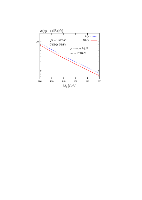
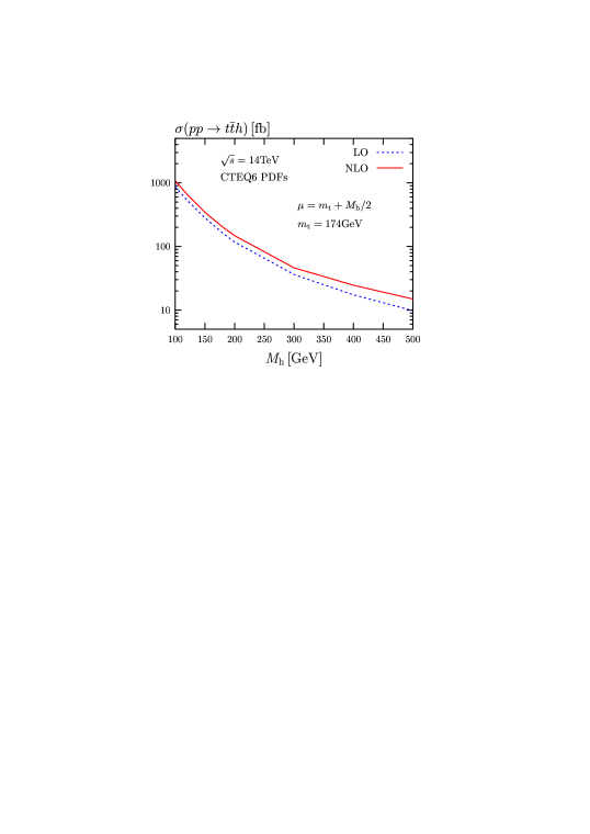
Figure 8.1.33: Total LO and NLO cross sections for $pp,p\overline{p}\to t\bar{t}h$ as functions of $M_{h}$, at $\sqrt{s}\!=\!1.96$ TeV and $\sqrt{s}\!=\!14$ TeV, for $\mu\!=m_{t}+M_{h}/2$.

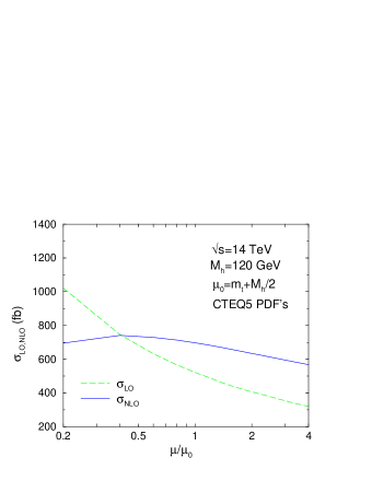
Figure 8.1.34: Dependence of $\sigma_{\scriptscriptstyle LO,NLO}(pp,p\bar{p}\to t\bar{t}h)$ on the renormalization/factorization scale $\mu$, at $\sqrt{s}\!=\!2$ TeV (l.h.s.)and $\sqrt{s}\!=\!14$ TeV (r.h.s.), for $M_{h}\!=\!120$ GeV.

The impact of NLO QCD corrections on the total cross section for $p\overline{p},pp\to t\bar{t}h$ production in the Standard Model is illustrated in Fig. 8.1.33[212, 44, 43, 210] and Fig. 8.1.34[212, 210]. The dependence of the total cross sections on the renormalization and factorization scales is strongly reduced at NLO as shown in Fig. 8.1.34. The numerical results at NLO are obtained using CTEQ4M (Fig. 8.1.34 (l.h.s.)), CTEQ5M (Fig. 8.1.34 (r.h.s.)), and CTEQ6M (Fig. 8.1.33) parton distribution functions. The NLO cross section is evaluated using the 2-loop evolution of $\alpha_{s}(\mu)$ with $\alpha_{s}^{NLO}(M_{Z})=0.116$ (Fig. 8.1.34 (l.h.s.)) and $\alpha_{s}^{NLO}(M_{Z})=0.118$ (Fig. 8.1.34 (r.h.s.)) and Fig. 8.1.33), and $m_{t}=174$ GeV. The renormalization/factorization scale dependence, uncertainty on the PDFs, and the error on the top quark pole mass, $m_{t}$, are estimated to give a 15-20$\%$ uncertainty.

8.2 Results for $b\bar{b}h$ Production

The $b\bar{b}h$ production processes are only relevant discovery modes in the MSSM with large $\tan\beta$. To a good approximation, the predictions for the MSSM rates can easily be derived from the Standard Model results by rescaling the Yukawa couplings[40]. The dominant MSSM radiative correction to $b\bar{b}h$ production can be taken into account by including the MSSM corrections to the $b\bar{b}h$ vertex only, i.e. by replacing the tree level Yukawa couplings by the radiative corrected ones. We follow the treatment of the program FeynHiggs [219, 112] and take into account the leading, $\tan\beta$ enhanced, radiative corrections that are generated by gluino-sbottom and chargino-stop loops. For large $\tan\beta$, the bottom quark Yukawa coupling is enhanced and the top quark Yukawa coupling coupling is strongly suppressed, resulting in a MSSM $b\bar{b}h$ cross section that is about three orders of magnitude larger than the Standard Model cross section. For the Tevatron, we calculate the production rates for the lightest MSSM Higgs boson, $h^{0}$, while for the LHC we consider the rate for the heavier neutral Higgs boson, $H^{0}$.

In the numerical evaluation of cross sections for the exclusive and semi-inclusive channels ($b{\overline{b}}h$ and $bh+\bar{b}h$ production), it is required that the final state bottom quarks have $p_{T}\!>\!20~{}$GeV and pseudorapidity $\mid\!\eta\!\mid<\!2.0$ for the Tevatron and $\mid\!\eta\!\mid<\!2.5$ for the LHC. In the NLO real gluon emission contributions, the final state gluon and bottom quarks are considered as separate particles only if their separation in the pseudorapidity-azimuthal angle plane, $\Delta R\!=\!\sqrt{(\Delta\eta)^{2}+(\Delta\phi)^{2}}$, is larger than $0.4$. For smaller values of $\Delta R$, the four momentum vectors of the two particles are combined into an effective bottom/anti-bottom quark momentum four-vector.

If not stated otherwise, the numerical results at NLO are obtained using CTEQ6M PDFs, the 2-loop evolution of $\alpha_{s}(\mu)$ with $\alpha_{s}^{NLO}(M_{Z})=0.118$, and the $\overline{MS}$ renormalization scheme for the bottom quark mass and Yukawa coupling with 2-loop renormalization group improved $\overline{MS}$ masses. The bottom quark pole mass is chosen to be $m_{b}=4.62$ GeV.

8.3 Total Cross Sections for $b\bar{b}h$ Production

We present total cross section results at NLO in the 4FNS in Fig. 8.3.35 for associated $b\bar{b}$ Higgs production in the MSSM with $\tan\beta=40$. The bands represent the theoretical uncertainty due to the residual scale dependence. They have been obtained by varying the renormalization ($\mu_{r}$) and factorization ($\mu_{f}$) scales independently from $\mu_{0}/4$ to $\mu_{0}$, where $\mu_{0}\!=\!m_{b}+M_{h}/2$.

If the outgoing bottom quarks cannot be observed then the dominant MSSM Higgs production process at large $\tan\beta$ is $gg\rightarrow(b\bar{b})h$ (the curve labelled ’0 b’). The inclusive cross section is experimentally relevant only if the Higgs boson can be detected above the background without tagging bottom quarks. At the LHC, this process can be identified at large $\tan\beta$ by the decays to $\mu^{+}\mu^{-}$ and $\tau^{+}\tau^{-}$ for the heavy Higgs bosons, $H^{0}$ and $A^{0}$, of the MSSM. At the Tevatron this process, with $h^{0}\rightarrow\tau^{+}\tau^{-}$, has been used to search for the neutral MSSM Higgs boson. If a single bottom quark is tagged then the final state is $bh$ or $\bar{b}h$ (the curve labelled ’1 b’). Although requiring a $b$ quark in the final state significantly reduces the rate, it also reduces the background. A recent Tevatron study [88] used the search for neutral MSSM Higgs bosons in events with three bottom quarks in the final state ($bh^{0}+\bar{b}h^{0}$ production with $h^{0}\rightarrow b\bar{b}$) to impose limits on the $\tan\beta$ and $M_{A^{0}}$ parameter space.

Finally, we show the fully exclusive cross sections for $b\bar{b}h$ production, where both the outgoing $b$ and $\bar{b}$ quarks are identified (the curve labelled ’2 b’). The exclusive measurement corresponds to the smallest cross section, but it also has a significantly reduced background. Moreover, both the exclusive and semi-inclusive $b\bar{b}h$ production modes are the only ones that can unambiguously measure the bottom quark Yukawa coupling.

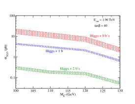
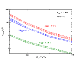
Figure 8.3.35: Total cross sections for $pp,p\bar{p}\rightarrow b\bar{b}h$ in the MSSM in the 4FNS at NLO for the Tevatron and the LHC in the MSSM with $\tan\beta=40$ and with 0,1 or 2 $b$ quarks identified. The Tevatron (LHC) plot is for the lightest (heaviest) neutral Higgs boson, $h^{0}$ ($H^{0}$). The error bands have been obtained by varying the renormalization and factorization scales as described in the text.

8.4 Differential Cross Sections for $b\bar{b}h$ Production

In assessing the impact of the NLO corrections it is particularly interesting to study the kinematic distributions. In Figs. 8.4.36 and 8.4.37 we illustrate the impact of NLO QCD corrections on the transverse momentum and pseudorapidity distribution of the SM Higgs boson and the bottom quark by showing the relative correction, $d\sigma_{NLO}/d\sigma_{LO}-1$ (in percent) for the exclusive case ($b{\overline{b}}h$ where both $b$ quarks are observed). For the renormalization/factorization scale we choose $\mu=2\mu_{0}$ at the Tevatron and $\mu=4\mu_{0}$ at the LHC, with $\mu_{0}=m_{b}+M_{h}/2$, and use the CTEQ5 set of PDFs. As can be seen, the NLO QCD corrections can considerably affect the shape of kinematic distributions, and their effect cannot be obtained from simply rescaling the LO distributions with a K-factor of $\sigma_{\scriptscriptstyle NLO}/\sigma_{\scriptscriptstyle LO}\!=\!1.38\pm 0.02$ (Tevatron, $\mu\!=\!2\mu_{0}$) and $\sigma_{\scriptscriptstyle NLO}/\sigma_{\scriptscriptstyle LO}\!=\!1.11\pm 0.03$ (LHC, $\mu\!=\!4\mu_{0}$).

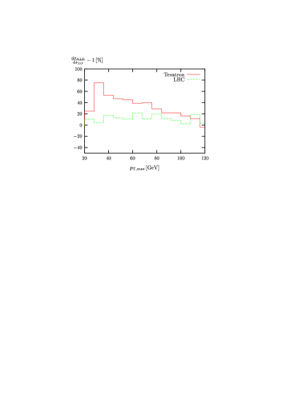
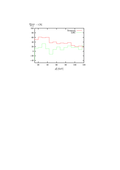
Figure 8.4.36: The relative corrections $d\sigma_{\scriptscriptstyle NLO}/d\sigma_{\scriptscriptstyle LO}-1$ for the $p_{T}$ distribution of the bottom or anti-bottom quark with the largest $p_{T}$ ($p_{T,max}$) (left) and of the SM Higgs boson ($p_{T}^{h}$) (right) to $b\bar{b}h$ production in the SM at the Tevatron (with $\sqrt{s}\!=\!2$ TeV and $\mu\!=\!2\mu_{0}$) and the LHC (with $\sqrt{s}\!=\!14$ TeV and $\mu\!=\!4\mu_{0}$).

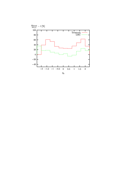
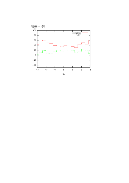
Figure 8.4.37: The relative corrections $d\sigma_{\scriptscriptstyle NLO}/d\sigma_{\scriptscriptstyle LO}-1$ for the $\eta$ distribution of the bottom quark $\eta_{b}$ (left) and of the SM Higgs boson ($\eta_{h}$) (right) to $b\bar{b}h$ production in the SM at the Tevatron (with $\sqrt{s}\!=\!2$ TeV and $\mu\!=\!2\mu_{0}$) and the LHC (with $\sqrt{s}\!=\!14$ TeV and $\mu\!=\!4\mu_{0}$).

8.5 PDF and Renormalization/Factorization Scale Uncertainties

A major source of theoretical uncertainty for cross section predictions comes from the PDFs. We study the uncertainties of semi-inclusive $bh$ production rates from the uncertainties in the PDFs using the CTEQ PDF sets[32]. First, the central value cross section $\sigma_{0}$ is calculated using the global minimum PDF (i.e. CTEQ6M). The calculation of the cross section is then performed with the additional 40 sets of PDFs to produce 40 different predictions, $\sigma_{i}$. For each of these, the deviation from the central value is calculated to be $\Delta\sigma_{i}^{\pm}=|\sigma_{i}-\sigma_{0}|$ when ${\sigma_{i}}_{<}^{>}\sigma_{0}$. Finally, to obtain the uncertainties due to the PDFs the deviations are summed quadratically as $\Delta\sigma^{\pm}=\sqrt{\sum_{i}{\Delta\sigma^{\pm}_{i}}^{2}}$ and the cross section including the theoretical uncertainties arising from the PDFs is quoted as $\sigma_{0}|^{+\Delta\sigma^{+}}_{-\Delta\sigma^{-}}$.

In Fig. 8.5.38, we plot the normalized total SM NLO cross sections for semi-inclusive $bh$ production, calculated in the 5FNS ($bg\rightarrow bh$) as implemented in MCFM [220] and in the 4FNS ($gg\rightarrow b(\bar{b})h$), and compare their respective uncertainties due to the PDFs. We see that, at both the Tevatron and the LHC, the PDF uncertainties are almost identical for both the $gg$ and $bg$ initial states.

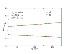
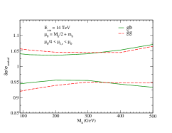
Figure 8.5.38: Normalized cross sections for Higgs production with one $b$ jet at the Tevatron (l.h.s) and the LHC (r.h.s) showing the uncertainty from PDFs for both the $gg$ (4FNS) and $bg$ (5FNS) initial states.

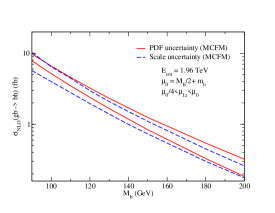
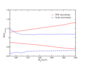
Figure 8.5.39: Comparison between theoretical uncertainties due to scale dependence and uncertainties arising from the PDFs at the Tevatron for semi-inclusive $bh$ production in the Standard Model. In the right-hand plot, both uncertainty bands have been normalized to the central value of the total cross section $\sigma_{0}$.

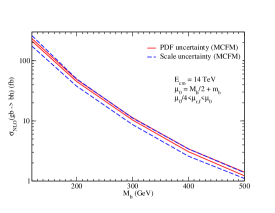
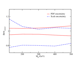
Figure 8.5.40: Comparison between theoretical uncertainties due to scale dependence and uncertainties arising from the PDFs at the LHC for semi-inclusive $bh$ production in the Standard Model. In the bottom plot, both uncertainty bands have been normalized to the central value of the total cross section $\sigma_{0}$.

In Figs. 8.5.39 and 8.5.40 we compare the uncertainties from residual scale dependence and the PDFs on the example of $bg\rightarrow bh$ (5FNS) at the Tevatron and LHC respectively[40]. Here, we perform the comparison for both the total cross section (left) and the total cross section normalized to the central value calculated with CTEQ6M (right). Similar results are obtained in the 4FNS.

From Fig. 8.5.40 one can see that, at the LHC, the theoretical uncertainty is dominated by the residual scale dependence. Due to the large center of mass (c.o.m.) energy of the LHC, the gluons and bottom quarks in the initial state have small momentum fraction ($x$) values and, hence, small PDF uncertainties typically in the 5-10% range.

In contrast, due to the smaller c.o.m. energy, the PDF uncertainties at the Tevatron (Fig. 8.5.39) are comparable and even larger than the uncertainties due to residual scale dependence over the full Higgs mass range. The smaller c.o.m. energy results in higher-$x$ gluons and bottom quarks in the initial state which corresponds to large PDF uncertainties in the 10-30% range.

8.6 Conclusion

The NLO cross sections for $t{\overline{t}}h$ and $b{\overline{b}}h$ have been presented for the Tevatron and the LHC with emphasis on the renormalization/factorization scale and PDF dependences.

Acknowledgments

The work of S.D. and C.J. ( L.R) is supported in part by the U.S. Department of Energy under grant DE-AC02-98CH10886 (DE-FG-02-91ER40685). The work of D.W. is supported in part by the National Science Foundation under grant No. PHY-0244875.

9 Heavy-flavor effects in supersymmetric Higgs boson production at hadron colliders

Contributed by: A. Belyaev, S. Berge, P.M. Nadolsky, F.I. Olness, C.P. Yuan

The Higgs sector may be represented by one complex scalar doublet, as it is economically realized in the Standard Model (SM), or by two or more doublets, as it takes place in the Minimal Supersymmetric Standard Model (MSSM) and its extensions. An important feature of MSSM is that, for large values of $\tan\beta$, the Yukawa couplings of the $b$-quarks to the neutral Higgs bosons $m_{H}$ (where $m_{H}=h$, $H$, or $A$) are strongly enhanced compared to the SM $b\bar{b}H_{SM}$ Yukawa coupling. Consequently, production of supersymmetric Higgs bosons in $b\bar{b}$ fusion can have a large cross section in supersymmetric extensions of the Standard Model [221, 222, 35, 223, 224].

The partonic processes contributing to the inclusive Higgs boson production with enhanced $b\bar{b}m_{H}$ coupling are represented by (a) $b\bar{b}\rightarrow m_{H}$; (b) $gb\rightarrow m_{H}b$; and (c) $gg\rightarrow b\bar{b}m_{H}$ scattering. The three processes (a,b,c) all give rise to the same hadronic final states, with two $B$-mesons appearing in different, but overlapping, regions of phase space. The distinction between the three processes depends very much on the factorization scheme adopted for the QCD calculation, as has been recently reviewed in Ref. [225].

As shown in Refs. [62, 76], the correct model for the transverse momentum distribution of the Higgs boson is crucial for unambiguous reconstruction of the Higgs boson mass in the $m_{H}\rightarrow\tau\tau$ decay channel. It is also important for discriminating the signal events from the backgrounds by examining the $q_{T}$ distribution of the Higgs boson in ${m_{H}}b\bar{b}$ associated production, followed by ${m_{H}}\rightarrow b\bar{b}$ decay [4]. The transverse momentum ($q_{T}$) distributions of Higgs bosons may be sensitive to the mass $m_{b}$ of the bottom quark when $q_{T}$ is comparable to $m_{b}$. In Refs. [226, 201] , we study the effect of the initial-state multiple parton radiation and heavy-quark masses on the transverse momentum distribution in the $b\bar{b}\rightarrow m_{H}$ process. Here we summarize the results of those two papers.

9.1 Transverse Momentum Resummation for Massive Quarks

The resummed differential cross section for inclusive production of Higgs bosons in scattering of initial-state hadrons $A$ and $B$ takes the form [205]

$$\frac{d\sigma}{dQ^{2}dydq_{T}^{2}}=\int_{0}^{\infty}\frac{{\rm b}d{\rm b}}{2\pi}\,J_{0}(q_{T}{\rm b})\,W({\rm b},Q,x_{A},x_{B},m_{b})\,\,+\,\,Y(q_{T},Q,y,m_{b}),$$ (9.1.64)

where $y$ is the rapidity of the Higgs boson, $x_{{A,B}}\equiv Qe^{\pm y}/\sqrt{S}$ are the Born-level partonic momentum fractions, $S$ is the square of the center-of-mass energy of the collider, and $J_{0}(q_{T}{\rm b})$ is the Bessel function. The resummed form factor $W$ is given in impact parameter ($\mathrm{b}$) space and factorizes as

$$W({\rm b},Q,x_{{A}},x_{{B}},m_{b})=\frac{\pi}{S}\,\sum_{j,k}\sigma_{jk}^{(0)}\,e^{-\mathcal{S}({\rm b},Q,m_{b})}\,\,{\mathcal{\overline{P}}}_{j/A}(x_{A},{\rm b},m_{b})\,\,{\mathcal{\overline{P}}}_{k/B}(x_{{B}},{\rm b},m_{b}),$$ (9.1.65)

where the summation is performed over the relevant parton flavors $j$ and $k$. Here, $\sigma_{jk}^{(0)}$ is a product of the Born-level prefactors, $e^{-{\mathcal{S}}({\rm b},Q,m_{b})}$ is an exponential of the Sudakov integral

$${\mathcal{S}}({\rm b},Q,m_{b})\equiv\int_{b_{0}^{2}/{\rm b}^{2}}^{Q^{2}}\frac{d\bar{\mu}^{2}}{\bar{\mu}^{2}}\biggl{[}{\mathcal{A}}(\alpha_{s}(\bar{\mu}),m_{b})\,\mathrm{ln}\biggl{(}\frac{Q^{2}}{\bar{\mu}^{2}}\biggr{)}+{\mathcal{B}}(\alpha_{s}(\bar{\mu}),m_{b})\biggr{]},$$ (9.1.66)

with $b_{0}\equiv 2e^{-\gamma_{E}}\approx 1.123$, and ${\mathcal{\overline{P}}}_{j/A}(x,{\rm b},m_{b})$ are the ${\rm b}$-dependent parton distributions for finding a parton of type $j$ in the hadron $A$. In the perturbative region (${\rm b}^{2}\ll\nolinebreak\Lambda_{QCD}^{-2}$), the distributions ${\mathcal{\overline{P}}}_{j/A}(x,\mathrm{b},m_{b})$ factorize as

$$\left.\overline{{\mathcal{P}}}_{j/A}(x,\mathrm{b},m_{b})\right|_{\mathrm{b}^{2}\ll\Lambda_{QCD}^{-2}} = \sum_{a=g,u,d,...}\,\int_{x}^{1}\,\frac{d\xi}{\xi}\,{\mathcal{C}}_{j/a}(x/\xi,\mathrm{b},m_{b},\mu_{F})\,f_{a/A}(\xi,\mu_{F})$$ (9.1.67)

into a convolutions of the Wilson coefficient functions ${\mathcal{C}}_{j/a}(x,\mathrm{b},m_{b},\mu_{F})$ and $k_{T}$-integrated parton distributions $f_{a/A}(\xi,\mu_{F})$. The Sudakov exponential and ${\rm b}$-dependent parton densities resum contributions from soft and collinear multi-parton radiation, respectively. $Y\equiv\mbox{PERT}-\mbox{ASY}$ is the difference between the finite-order cross section (PERT) and its asymptotic expansion in the small-$q_{T}$ limit (ASY).

The Higgs cross sections depend on the mass $m_{b}$ of the bottom quark. The distributions $\overline{{\mathcal{P}}}_{j/A}(x,{\rm b},m_{b})$ for the heavy quarks ($j=c,b$) cannot be reliably evaluated at all impact parameters if a conventional factorization scheme, such as the zero-mass variable-flavor number (ZM-VFN, or massless) scheme, is used. The reason is that $m_{b}$ acts as an additional large momentum scale, which, depending on the value of ${\rm b}$, introduces large logarithms $\ln^{n}(m_{b}{\rm b})$ or non-negligible terms $\propto(m_{b}{\rm b})^{n}$. The situation encountered here is reminiscent of the heavy-quark contributions to the DIS structure functions $F_{i}(x,Q^{2}),$ which are not adequately described by the conventional factorization schemes at either small or large momentum transfers $Q^{2}$ (see, for instance, [227]). To work around this complication, Ref. [228] proposed to formulate the CSS formalism in a general-mass variable flavor number (GM-VFN) scheme [229], which correctly evaluates the heavy-quark mass effects at all momentum scales. Among all GM-VFN factorization schemes, the S-ACOT scheme [229, 230] was found to be well-suited for the efficient calculation of the CSS resummed cross sections. In particular, in this heavy-quark CSS (CSS-HQ) formalism [228] the dependence on $m_{b}$ is dropped in all ${\cal O}(\alpha_{s})$ terms in Eq. (9.1.64) except for $\overline{{\mathcal{P}}}_{b/A}(x,{\rm b},m_{b})$.

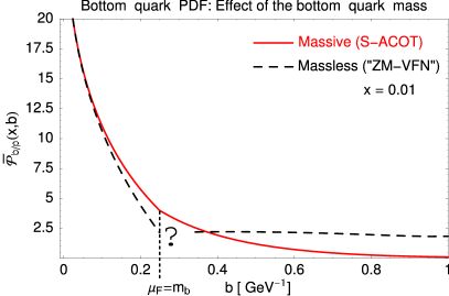
Figure 9.1.41: The bottom-quark distributions $\overline{{\mathcal{P}}}_{b/p}(x,{\rm b},m_{b})$ in the proton vs. the impact parameter ${\rm b}$. The solid and dashed curves correspond to the S-ACOT and massless (“ZM-VFN”) factorization schemes, respectively.

The dependence of the bottom-quark parton density $\overline{{\mathcal{P}}}_{b/p}(x,{\rm b},m_{b})$ on the impact parameter is shown in Fig. 9.1.41. The ZM-VFN parton density $\overline{{\mathcal{P}}}_{b/p}(x,{\rm b},m_{b})$ is not properly defined below the threshold $\mu_{F}=m_{b}$ (or above ${\rm b}=b_{0}/m_{b}$). It was continued to large ${\rm b}$ in the previous calculations using an effective “ZM-VFN” approximation described in Ref. [226]. The S-ACOT parton density $\overline{{\mathcal{P}}}_{b/p}(x,{\rm b},m_{b})$ is well-defined at all ${\rm b}.$ It reduces to the ZM-VFN result at ${\rm b}\ll b_{0}/m_{b}$ and is strongly suppressed at ${\rm b}\gg b_{0}/m_{b}$. The suppression is caused by the decoupling of the heavy quarks in the parton densities at $\mu_{F}$ much smaller than $m_{b}$ (${\rm b}$ much larger than $b_{0}/m_{b}$). Consequently the impact of the non-perturbative contributions from ${\rm b}\gtrsim 1\mbox{\, GeV}^{-1}$ is reduced in the heavy-quark channels compared to the light-quark channels.

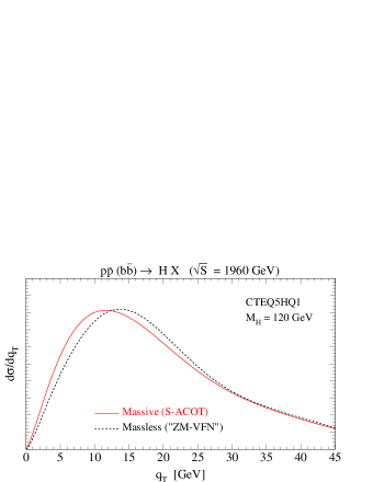
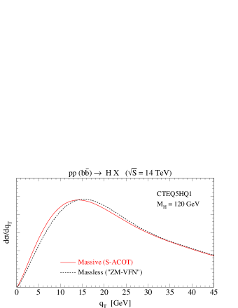
(a)                                                                (b)

Figure 9.1.42: Transverse momentum distribution of on-shell Higgs bosons in the $b\bar{b}\to m_{H}$ channel at (a) the Tevatron and (b) LHC. The solid (red) lines show the $q_{T}$ distribution in the massive (S-ACOT) scheme. The dashed (black) lines show the distribution in the massless (“ZM-VFN”) scheme. The numerical calculation was performed using the programs Legacy and ResBos [231, 232] with the CTEQ5HQ1 parton distribution functions [233]. The bottom quark mass is taken to be $m_{b}=4.5$ GeV.

The massless (“ZM-VFN”) calculation therefore underestimates the true behavior at ${\rm b}>\nolinebreak 0.1\mbox{ GeV}^{-1}$ and small $q_{T}$. This effect can be seen in Fig. 9.1.42, which displays $d\sigma/dq_{T}$ for $b\bar{b}\rightarrow m_{H}$ boson production at (a) the Tevatron and (b) LHC. At the Tevatron, the $q_{T}$ maximum shifts in the “ZM-VFN” approximation to larger $q_{T}$ by about $2$ GeV out of $11.7$ GeV (about $17\,$%). For a Higgs mass $M_{H}=200$ GeV, the maximum of $d\sigma/dq_{T}$ shifts by about 1.9 GeV out of $12.7$ GeV. At the LHC, the difference between the “ZM-VFN” and S-ACOT calculations is smaller compared to the Tevatron, because the influence of the ${\rm b}>0.1\,\mbox{GeV}^{-1}$ region is reduced at smaller momentum fractions $x$ probed at the LHC [234]. The maximum of the $q_{T}$ distribution shifts in the “ZM-VFN” approximation by about $1.3$ GeV (9% out of $14.1$ GeV) to larger $q_{T}$. The results for other Higgs masses can be found in Ref. [226].

9.2 Numerical Comparison with PYTHIA

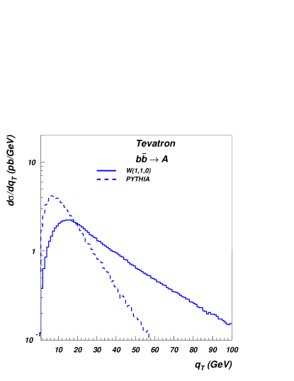
Figure 9.2.43: $q_{T}$ distributions for production of 100 GeV CP-odd Higgs bosons $A$ via $b\bar{b}$ fusion in the Tevatron Run-2. The solid and dashed curves correspond to the lowest-order $W$-term $W(1,1,0)$ (with functions ${\cal A}(\alpha_{s}(\bar{\mu}))$ and ${\cal B}(\alpha_{s}(\bar{\mu}))$ evaluated at ${\cal O}(\alpha_{s})$) and PYTHIA.

The full $q_{T}$ dependence of the $b\bar{b}\rightarrow m_{H}$ process is affected by constraints on phase space available for QCD radiation (less relevant at small $q_{T}$). We illustrate the interplay of various effects by comparing the CSS-HQ resummation to the PYTHIA Monte Carlo program [235]. We focus on production of the CP-odd Higgs particle $A$ for $\tan\beta=50$ (predictions for the other Higgs bosons can be obtained by rescaling the $b\bar{b}A$ coupling).

As compared to the CSS-HQ formalism, the PYTHIA calculation does not include contributions generated from the ${\cal C}$-functions and $Y$-term, and it evaluates the soft parton contributions at ${\cal O}(\alpha_{s}).$ Therefore, we start by comparing the PYTHIA $q_{T}$ distribution to the resummed $W$-term $W(1,1,0)$ in Eq. (9.1.64), with the functions ${\cal A},$ ${\cal B}$, and ${\cal C}$ in Eqs. (9.1.66), (9.1.67) being evaluated at orders $\alpha_{s},$ $\alpha_{s}$, and $\alpha_{s}^{0}$, respectively. The orders of $\alpha_{s}$ in ${\cal A},$ ${\cal B}$, and ${\cal C}$ are shown as the arguments of $W(1,1,0)$.

It is evident from Fig. 9.2.43 that the shapes of $W(1,1,0)$ and PYTHIA $q_{T}$ distribution are very different, though the integrated rates (i.e., the areas under the two curves) are about the same. The $q_{T}$ distribution from PYTHIA is narrower and peaks at lower $q_{T}$ than $W(1,1,0)$. The large discrepancy between the two curves is in contrast to the case of $W$ and $Z$ production via light-quark scattering, where the above two calculations predict similar, though not identical, $q_{T}$ distributions [231].

A closer examination reveals that additional features must be implemented in the resummed cross section in order to reliably describe the $q_{T}$ distributions of Higgs bosons produced via $b\bar{b}$ fusion.

• The kinematical effects account for a large part of the disparity between $W(1,1,0)$ and PYTHIA. The bottom-quark PDF is a rapidly decreasing function of $x$ in the probed range of $x$. Consequently, approximations for the true partonic kinematics (especially those made for the light-cone momentum fractions $x$) may have a strong impact on the rate of $b\bar{b}$ scattering. This feature should be contrasted to the behavior of the light-quark PDF’s in $W$ and $Z$ production, which include a substantial valence component and vary slower with $x$. As a result, the kinematical approximations are less consequential in the $W$ and $Z$ case.
   
  When PYTHIA generates QCD radiation, the kinematical distributions of the final-state particles, including the quarks and gluons from the QCD showering, are modified to satisfy energy-momentum conservation at each stage of the showering. In the resummation calculation, information about the exact parton kinematics is included in the finite-order term (PERT). The resummed cross section is therefore expected to be closer to PYTHIA once the ${\cal O}(\alpha_{s})$ finite term, PERT(1)-ASY(1), is included. In the $W(1,1,0)$ calculation, the emitted gluons are assumed not to carry any momentum at all in the soft limit. To compensate for small, but nonzero energy of the soft gluon emissions, we introduce a “kinematical correction” (KC) in the W and ASY terms. This correction modifies the minimal values of partonic momentum fractions $x_{A}$ and $x_{B}$ in order to account for reduction of phase space available for collinear QCD radiation at large $q_{T}$.

• The lowest-order cross section $W(1,1,0)$ does not evaluate effects of the bottom-quark mass, which is first included in the ${\cal C}$-function of order $\alpha_{s}$. Also, additional, though not complete, $O(\alpha_{s}^{2})$ contributions arise in the Sudakov form factors inside PYTHIA when the next-to-leading order PDF’s are used. To account for both features, we evaluate the $W$ term at one higher order (2,2,1) and include the $m_{b}$ dependence using the CSS-HQ scheme.

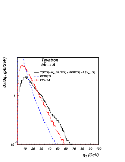
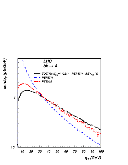
(a)                                                                  (b)

Figure 9.2.44: Comparison of $q_{T}$ distributions predicted by TOT(1), PERT(1) and PYTHIA, for Higgs boson produced via $b\bar{b}$ fusion at (a) the Tevatron Run-2 and (b) LHC, for $M_{A}=$100 and 300 GeV respectively.

Thus, our full prediction TOT(1) is obtained by adding ${\textrm{W}}_{\textrm{KC}}^{\textrm{CSS-HQ}}$(2,2,1) (evaluated in the CSS-HQ formalism with the kinematical correction) and PERT(1), and subtracting ${\textrm{ASY}}_{\textrm{KC}}$(1). It is shown for $M_{A}=100$ GeV at the Tevatron in Fig. 9.2.44(a) and $M_{A}=300$ GeV at the LHC in Fig. 9.2.44(b). TOT(1) (solid line) is compared to the fixed-order prediction PERT(1) (dashed) and the PYTHIA prediction (dot-dashed). As one can see, the results for Tevatron and LHC are qualitatively similar. TOT(1) is closer to the PYTHIA prediction than $W(1,1,0)$, though the two distributions are not identical. The PYTHIA $q_{T}$ distribution peaks at lower $q_{T}$ than TOT(1). In the large $q_{T}$ region, the TOT(1) rate is larger than the PYTHIA rate.

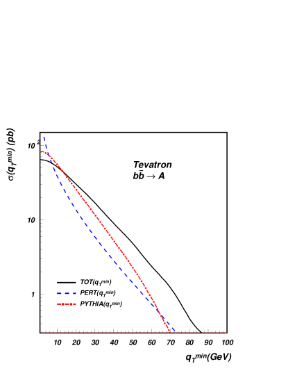
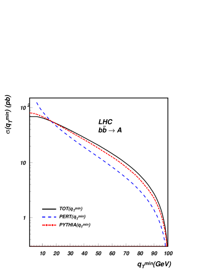
Figure 9.2.45: Comparison of the integrated rates, deduced form Fig. 9.2.44, as a function of the minimal $q_{T}$ value taken in the integration over $q_{T}$ at the Tevatron Run-2 (left) and LHC (right) for $M_{A}=$100 and 300 GeV, respectively.

Finally, Fig. 9.2.45 shows the integrated cross section as a function of the minimal $q_{T}$ in the calculation for the Tevatron (left) and LHC (right). This is another way to illustrate the differences in the shapes of $q_{T}$ distributions obtained in the resummation, fixed-order, and PYTHIA calculations.

9.3 Conclusion

Multiple parton radiation in $b$-quark scattering is conspicuously sensitive to effects of large bottom-quark mass $m_{b}$ and phase-space constraints on collinear emissions. Both $m_{b}$ dependence and phase-space dependence tangibly modify the shape of Higgs $q_{T}$ distributions in the $b\bar{b}\rightarrow m_{H}$ processes. The two types of effects were consistently implemented within the CSS resummation formalism for heavy-quark scattering [228, 226, 201], realized in a massive (GM-VFN) factorization scheme. These corrections act on different $q_{T}$ regions. When the dependence on $m_{b}$ is taken into account, the position of the peak in the $d\sigma/dq_{T}$ distribution shifts to a lower $q_{T}$ value, leaving the rate at large $q_{T}$ essentially unchanged. The kinematical correction is effective in the high-$q_{T}$ region, where it largely reduces the Higgs production rate. As a result, we obtain an improved prediction for the full $q_{T}$ spectrum of Higgs bosons, an important piece of information needed for the future Higgs searches.

Acknowledgments

This work was supported in part by the U.S. Department of Energy under grant DE-FG03-95ER40908, contract W-31-109-ENG-38, and the Lightner-Sams Foundation. We also acknowledge the support in part by the U.S. National Science Foundation under awards PHY-0354838 and PHY-0244919.

10 Higgs Signal for $h\rightarrow aa$ at the Tevatron

Contributed by: M. Carena, T. Han, G.-Y. Huang, C.E.M Wagner

The elucidation of the mechanism leading to the origin of mass of all observed elementary particles is one of the main goals in high energy physics. The simple Standard Model (SM) picture, based on the spontaneous breakdown of the electroweak symmetry by the vacuum expectation value of an elementary Higgs field, seems to lead to a picture that is consistent with all experimental observables, provided the Higss boson mass is smaller than about 250$\mathrm{\ Ge\kern-1.00006ptV}$. Moreover, the best fit to the precision electroweak observables measured at the LEP, SLC and Tevatron experiments lead to values of the Higgs mass of the order of or smaller than the present bound coming from direct searches at LEP, $m_{H_{\rm SM}}\gtrsim 114\mathrm{\ Ge\kern-1.00006ptV}$.

In spite of the extraordinary good agreement of the experimental observations with the standard model predictions, there are many theoretical motivations to go beyond the Standard Model description. Several extensions of the Standard Model exist in the literature, and in most of them the Higgs sector is extended to a more complicated structure, often including at least two Higgs doublets. The requirement of preserving the good agreement with experimental data can be easily fulfilled in extensions, like supersymmetry, in which the effect of the additional particles on the precision electroweak observables rapidly vanish with increasing values of the new particle masses. Independently of the particular extension, the direct and indirect limits on the Higgs mass must be revised. In particular, the direct search for Higgs bosons may be affected by additional decay modes that are beyond the ones analysed by the LEP collaborations.

As an example, let us consider the minimal supersymmetric extension of the Standard Model (MSSM). In the MSSM, there is an additional Higgs doublet, leading, in the absence of CP-violation in the Higgs sector, to two CP-even and one CP-odd Higgs boson states. At large values of $\tan\beta$, the ratio of the v.e.v. of the two Higgs doublets, one of the CP-even Higgs bosons acquires Standard Model properties, while the second Higgs boson may only be produced in association with the CP-odd Higgs boson state. In addition, the masses of the non-standard CP-even Higgs and the CP-odd Higgs are close to each other. Under these conditions, the mass bound on the SM-like CP-even Higgs is similar to the SM one, while the CP-odd and the second CP-even Higgs boson mass bound reads $m_{h}>90\mathrm{\ Ge\kern-1.00006ptV}$ [236].

In this note, we will depart from these simple assumptions, by breaking the mass relations that appear in the simplest supersymmetric models, and studying the consequences of such modifications of the parameters of the theory. Indeed, while it has been a common belief that the Higgs boson will be eventually discovered at the upcoming LHC experiments, one would like to fully utilize the potential to search for the Higgs bosons at the Tevatron in these non-conventional scenarios as well. Non-standard mass relations are already present in extensions of the MSSM including an additional singlet (NMSSM) [237], or when explicit CP-violations exist in the Higgs sector [238]. In these cases, the SM-like Higgs ($h$) may dominantly decay into a pair of lighter Higgs ($a$), often the CP odd state. Therefore it is possible that the Higgs escaped detection at the LEP experiments by avoiding the usual decay modes such as $h\to 2b,\ 2\tau,\ WW^{*}$ and $ZZ^{*}$, and the lower limit on Higgs mass should be re-evaluated [239]. We are interested in analysing the sensitivity of the Tevatron experiments in the search for a light, SM-like Higgs boson with such an exotic decay mode. In particular, we will consider the case when the Higgs boson decays into a pair of scalars $h\to aa$, which in turn cascade into a heavy fermion pair $a\to b\bar{b}$ and $a\to\tau\bar{\tau}$, respectively.

The dominant production of the Higgs boson at hadron colliders comes from the gluon fusion, but the above channel would encounter huge SM backgrounds. We therefore consider the Higgs signal produced in association with a $W$ or $Z$ boson, in the hope that the leptonic decays of the weak bosons will provide a clean trigger, and will significantly reduce the background as well. The events being searched are

$$Wh\to l\nu_{l},aa \to\left\{\begin{array}[]{l}l\nu_{l},b\bar{b},b\bar{b}\\ l\nu_{l},b\bar{b},\tau\bar{\tau}\end{array}\right.$$ (10.0.70)

$$Zh\to l^{+}l^{-},aa \to\left\{\begin{array}[]{l}l^{+}l^{-},b\bar{b},b\bar{b}\\ l^{+}l^{-},b\bar{b},\tau\bar{\tau},\end{array}\right.$$ (10.0.73)

with $l=e,\mu$.

10.1 Parameter Choices

We would like to perform a relatively model-independent search for the typical signal. The direct search for a Higgs boson with SM-like couplings to the gauge bosons, in a model and decay mode-independent way, leads to a lower bound on $m_{h}$ of about 82$\mathrm{\ Ge\kern-1.00006ptV}$ [240]. Moreover, the proposed search is expected to become inefficient for $m_{h}>130\mathrm{\ Ge\kern-1.00006ptV}$, since the standard decays into the $WW^{*}$ and $ZZ^{*}$ channels are still expected to be dominant. Therefore, the optimal setting to detect the Higgs decaying into an $aa$ pair is to have the mass $m_{h}$ within the range of $90-130\mathrm{\ Ge\kern-1.00006ptV}$. The choice for $m_{a}$ can be more flexible. As long as $m_{a}>2m_{b}$ to kinematically allow the decay $a\to b\bar{b}$, our analyses are rather insensitive to the mass choices (see below for a more detailed analysis of this question).

In a generic model, the $Wh/Zh$ production rate differs from that in the SM. The change can be characterized by a prefactor $\kappa^{2}_{hWW}$ ($\kappa^{2}_{hZZ}$), where $\kappa_{hVV}$ is the coupling strength of Higgs to vector boson $V$ relative to that in the SM. The production cross section can thus be written in terms of the SM result with an overall factor to account for the modification of the coupling

$$\sigma(Vh)=\kappa^{2}_{hVV}\sigma^{SM}(Vh).$$ (10.1.74)

We are interested in the range of $\kappa\sim 0.5-1.0$, so that this Higgs contributes to the electroweak symmetry breaking and consequently the associated productions are still sizeable.

In order for the $h\to aa$ decay to be dominant and thus escape the LEP bound, $BR(h\to aa)$ is required to be close to unity. For instance, in the NMSSM, $BR(h\to aa)>0.9$ turns out to be very general in terms of the naturalness of $c$ in the trilinear coupling term $(cv/2)haa$ [241]. Moreover, if the down quark and lepton coupling to the Higgs is proportional to their masses, then $BR(a\to b\bar{b})$ and $BR(a\to\tau\bar{\tau})$ are set to be 0.92 and 0.08, respectively. In general, however, the relations between the coupling and the masses may be modified by radiative corrections, which can lead to a large increase of the $BR(h\to\tau\tau)$ [77]. The representative values and the ranges of the parameters are summarized in Table 10.1.8.

		representative	considered
	parameters	value	range
	$m_{h}$	120	90$-$130
masses	$m_{a}$	30	20$-$40
coupling	$\kappa_{hVV}$	0.7	0.5$-$1.0
	$BR(h\to aa)$	0.85	0.8$-$1.0
branching	$BR(a\to b\bar{b})$	0.92	0.95$-$0.70
fractions	$BR(a\to\tau\bar{\tau})$	0.08	0.05$-$0.30
$2b2\tau$	$C^{2}$	0.061	0.019$-$0.42

Table 10.1.8: Parameter choices for $h\to aa$ decays.

Including the decay branching fractions, for instance for $a_{1}\to b\bar{b},\ a_{2}\to\tau\bar{\tau}$, we obtain the cross section as

$$\sigma(aa)=\kappa^{2}_{hVV}\ \sigma^{SM}(Vh)\ BR(V)\ 2BR(h\to aa)BR(a\to b\bar{b})BR(a\to\tau\bar{\tau}).$$ (10.1.75)

where $BR(V)=0.213\ (0.067)$ is the leptonic branching ratio of the decay of $W\ (Z)$. into $l=e,\mu$.

The overall factor modifying the SM result in Eq. (10.1.75), i.e.

$$C^{2}\equiv 2\kappa^{2}_{hVV}BR(h\to aa)BR(a\to b\bar{b})BR(a\to\tau\bar{\tau}),$$ (10.1.76)

corresponds to the process-dependent $C^{2}$ factor defined in the DELPHI search [239]. Our parameter choice (range) is equivalent to a $C^{2}_{2b2\tau}$ of 0.061 (0.019$-$0.42), consistent with the bounds for a large range of our $m_{h},m_{a}$ choices set forth in Ref. [239] . A value of 0.061 for $C^{2}$ is assumed for all numerics from here on, unless explicitly noted otherwise.

10.2 Signal Event Rate

The associated production of $p\bar{p}\to Wh$ usually features a larger cross section than that of $Zh$, and the leptonic branching fraction of $W$ is about 3 times larger than $Z$’s. For illustration purposes, we choose to concentrate on the $Wh$ channel henceforth.

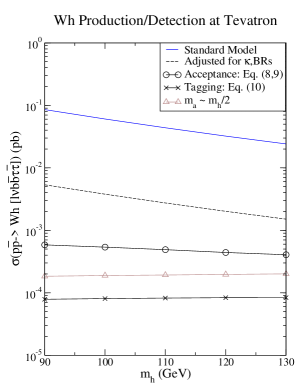
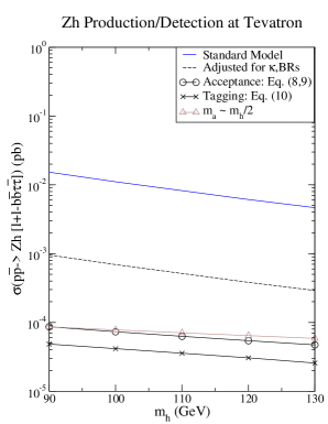
Figure 10.2.46: Cross sections of Higgs signal at the Tevatron in the $2b2\tau$ channel produced by Higgs-strahlung with a leptonically decaying $W$ (left) or $Z$ (right). $m_{a}=30\mathrm{\ Ge\kern-1.00006ptV}$ is assumed except for the two curves where $m_{a}=(m_{h}-10\mathrm{\ Ge\kern-1.00006ptV})/2$. $C^{2}=0.061$ is understood.

The Standard Model rate of a Higgs produced in association with a leptonically decaying $W$ is

$$\sigma^{SM}(Wh)\ BR(W\to l\nu_{l})\sim 85\ (24)\ {\rm fb}$$ (10.2.77)

at $\sqrt{s}=1.96$ TeV for $m_{h}=90\ (130)\mathrm{\ Ge\kern-1.00006ptV}$.

Including the branching fractions and couplings, the cross section of the signal in Eq. (10.1.75) is

$$\sigma(aa)\sim 5.3\ (1.5)\ {\rm fb\qquad for\quad}C^{2}=0.061$$ (10.2.78)

as illustrated in Fig. 10.2.46. The solid curve on top represents the total cross section for $Vh$ production, with $V$ decaying leptonically, but without any cuts. The dashed curve represents the cross section after adjusting for the couplings and branching fractions, as in Eq. (10.1.75). Cross sections for $Zh$ are also plotted for completeness.

The events have yet to pass the acceptance cuts, or to have the taus and $b$’s tagged. Both bring significant reductions to the event rate. Our challenges are to retain as many events as possible, and to control the backgrounds from various sources.

10.3 Background and Acceptance Cuts

We look for events with 5 particles plus missing energy in the final states: $b\bar{b}\tau\bar{\tau}l\nu_{l}$. We wish to trigger the events by the isolated lepton $l$, tag the $b$’s and $\tau$’s, and demand significant missing transverse energy ($\not\!\!E_{T}$) in the events. With neutrinos in the decay products, tau momenta cannot be fully reconstructed. Therefore we cannot reconstruct the invariant masses $m_{\tau\tau}$ or $m_{h}\sim m_{bb\tau\tau}$. Instead, the signal should appear as a peak in the $m_{bb}$ plot, around the value of $m_{a}$.

Acceptance Cuts

The following cuts are employed to mimic the detector acceptance:

$$p_{T} > 10\mathrm{\ Ge\kern-1.00006ptV}{\rm\qquad for}\ b,l^{\pm}$$

$$\not\!\!E_{T} > 10\mathrm{\ Ge\kern-1.00006ptV}{\rm\qquad for}\ Wh\ {\rm only}$$

$$|\eta| < 3.0\qquad\qquad{\rm for}\ b,l^{\pm}$$ (10.3.79)

$$\Delta R > 0.4\qquad\qquad{\rm for}\ bb,bl^{\pm}$$

$$m_{inv} > 20\mathrm{\ Ge\kern-1.00006ptV}{\rm\qquad for}\ bb,$$

and

$$p_{T} > 10,8,5\mathrm{\ Ge\kern-1.00006ptV}{\rm\qquad for}\ \tau_{h},\tau_{e},\tau_{\mu}$$

$$|\eta| < 1.5{\rm\qquad\qquad\qquad for}\ \tau$$ (10.3.80)

$$\Delta R > 0.4{\rm\qquad\qquad\qquad for}\ \tau\tau,\tau b,\tau l^{\pm}$$

$$m_{inv} > 10\mathrm{\ Ge\kern-1.00006ptV}{\rm\qquad\qquad for}\ \tau\tau,$$

where $\tau_{e}$,$\tau_{\mu}$ and $\tau_{h}$ stand for the decays of $\tau\to e\nu_{e}\nu_{\tau}$, $\tau\to\mu\nu_{\mu}\nu_{\tau}$, and $\tau\to\rm{hadrons}+\nu_{\tau}$, respectively. Lower cuts on $bb$ and $\tau\tau$ invariant masses are to eliminate the large number of background events from soft photons and gluons.

The momentum of the tau-lepton cannot be fully reconstructed since all tau decays involve at least one neutrino, therefore the cuts on tau are applied to the visible decay products, and are decay-mode dependent. After these acceptance cuts, $10-25$% of the signal events survive, and the cross section becomes $0.6\ (0.4)\$fb for $m_{h}=90\ (130)\mathrm{\ Ge\kern-1.00006ptV}$ with the given set of input parameters, or $C^{2}\sim 0.06$. The cross sections passing acceptance are plotted in Fig. 10.2.46 versus the Higgs mass, represented by the circled curve. There would be a few events to several tens of events with a few fb^-1 integrated luminosity, for $C^{2}\sim 0.019-0.42$.

Irreducible Background

The dominant source of the irreducible background the $b\bar{b}$ pair from a virtual gluon splitting, the $\tau\bar{\tau}$ pair from an intermediate $Z^{*}/\gamma^{*}$ and the charged lepton plus missing energy from a $W$ boson. Our Monte Carlo simulations with MadEvent [242] show that the $Z^{*}$ is almost on-shell. It can be readily removed with a cut on $\tau\bar{\tau}$ invariant mass. However as we shall see below, due to the small size of the background, we can afford not to do so. A $\tau\bar{\tau}$ pair from a virtual photon can be more easily confused with the signal, but such a background is further suppressed by the electromagnetic couplings.

After applying the acceptance cuts, the irreducible background is estimated to be around 0.01 fb, which is very small compared to the signal size. It is entirely absent given the luminosity at the Tevatron.

Reducible Background and Tagging

Taus and $b$’s need to be identified. During the identification (tagging), signal events are lost due to the tagging efficiency and to additional cuts. For example, the efficiency of tagging a single bottom is around 50% in the region $p_{T}>15\mathrm{\ Ge\kern-1.00006ptV}$, and falls off rapidly as we approach lower $p_{T}$. Tagging (hadronic) taus faces the same problem. Therefore tightening the kinematical cuts on $b$’s and taus are necessary to assure favorable tagging efficiencies. We decide to tag one $b$ and one tau.

The $b$- and hadronic $\tau$-tagging efficiencies are taken to be [243, 244]

$$b-tagging: 50\% {\rm for}\ E_{T}^{jet}>15\mathrm{\ Ge\kern-1.00006ptV}\ and\ |\eta_{jet}|<1.0\ ,$$

$$\tau-tagging: 40\% {\rm for}\ E_{vis}>20\mathrm{\ Ge\kern-1.00006ptV}\ and\ |\eta|<1.5\ .$$ (10.3.81)

Outside these kinematical regions, the tagging efficiencies drop sharply [243, 244].

Reducible background arise from jets mis-identified as $b$’s, or hadronically decaying taus. The mistag rate per jet is taken to be around $0.5-1.0$% ($0.5$%) for tau ($b$) [243, 244]. In addition, the experiments cannot distinguish directly produced electrons (muons) from leptonically decaying taus.

• The background due to misidentified bottom comes from the process $2\tau 2jl+\mbox{$\not\!\!E_{T}$}$, which has a cross section of 5 fb. Considering the mistag rate and the additional cuts, it contributes 0.01 fb to the background events.

• The background due to misidentified $\tau$ differs from the decay modes of $\tau$’s:

  • For $\tau_{l}\tau_{h}2bl\mbox{$\not\!\!E_{T}$}$ ($2l2b\tau_{h}\mbox{$\not\!\!E_{T}$}$), it comes from $2\tau 2bj$ with $\not\!\!E_{T}$ from the leptonic decays of both taus. The contribution is estimated at 0.003 fb.

  • For $\tau_{h}\tau_{h}2bl\mbox{$\not\!\!E_{T}$}$, the background comes from $2j2bl\mbox{$\not\!\!E_{T}$}$ estimated at $50$ fb after events of the $bb$ and $jj$ resonances around the $Z$ mass are rejected. It’s further reduced by a factor of $0.01-0.02$ from the tau-mistag rate, and a factor of 0.8 due to b-tagging.

    This results in a background rate of $0.4-0.8$ fb. In a continuum distribution of $m_{bb}$, it is at or below the level of the signal. We notice that the $b$ jets are harder in this background than in the signal (see Fig. 10.3.47). Imposing a upper $p_{T}$ cut of $50\mathrm{\ Ge\kern-1.00006ptV}$ will reduce the background by a factor of about 4, while the signal is minimally affected.

• The backgrounds from both a mistagged tau and a mistagged $b$ mostly come from the $4jl\mbox{$\not\!\!E_{T}$}$ events, which has a cross section of about 16 pb. After the cuts and folding in the mistag rates, this contributes $0.3-0.6$ fb of background events. It can be further reduced by imposing upper $p_{T}$ cuts, similarly to the $2j2bl\mbox{$\not\!\!E_{T}$}$ background.

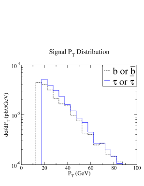
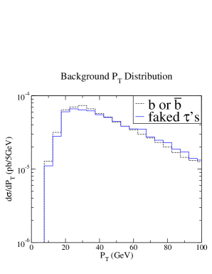
Figure 10.3.47: Transverse momenta distribution of the $b$, $\tau$ or jets in the $Wh$ signal (left) and background (right) events.

After carefully tightening the cuts, the reducible background can be a factor of a few to ten smaller than the signal, but unfortunately, the cuts and the tagging efficiencies together reduce the signal greatly to about 0.08 fb for $Wh$ and $0.03-0.05$ fb for $Zh$, with $C^{2}\sim 0.06$. With an optimistic $C^{2}\sim 0.42$, the cross section is 0.55 fb, we would expect to see about a couple of signal events with an integrated luminosity of a few fb^-1.

To illustrate a most optimistic situation, we explore the mass relations of $m_{a}$ and $m_{h}$. The signal loss is mainly due to the softness of the $b$ and $\tau$’s, therefore most events are rejected from the lower $p_{T}$ threshold. Increasing $m_{a}$ would stretch the $p_{T}$ distributions to the higher $p_{T}$ end. To achieve this without significantly affecting the decay phase space of $h$, we set

$$m_{a}=(m_{h}-10\mathrm{\ Ge\kern-1.00006ptV})/2,$$ (10.3.82)

which resulted in almost doubling the signal rate, as seen from the curve with triangles in Fig. 10.2.46. The cross section ($\sim 0.2\ {\rm fb}$ for $C^{2}=0.06$, and $\sim 1.4\ {\rm fb}$ for $C^{2}=0.42$) is still challenging for observation with the Tevatron’s projected luminosity.

10.4 Summary

The search for a Higgs boson with couplings to the gauge bosons of the order of the SM-one, and decaying into two lighter CP-odd Higgs bosons states may be performed at the Tevatron collider in the $Wh\to l\nu aa(2b2\tau)$ channel. For $90\leq m_{h}\leq 130\mathrm{\ Ge\kern-1.00006ptV}$, we found a sizable number of events, with negligible irreducible background. However, further cuts and tagging $b$ and $\tau$, necessary to remove the much larger reducible background worsen the signal event rate to the order 0.1 fb for a value of $C^{2}\sim 0.06$, a factor determined by the product of the relevant branching ratios times the ratio of the Higgs production cross section to the SM-one. Therefore, the signal observation becomes statistically limited. For an optimal choice of the value of the CP-odd Higgs mass $m_{a}$, the signal rate may be twice as large. With favorable couplings and branching fractions, the $C^{2}$ factor can be as large as 0.42, which would enhance the signal rate by a factor of 7 to around 1.4 fb. It can be further improved by another $40-60\%$ by combining $Zh$ events with the $Wh$ events, leading to a possible observation of a few events for a Tevatron luminosity of the order of a few fb^-1.

11 The $Z\to b\bar{b}$ decay as a b-jet energy calibration tool

Contributed by: T. Dorigo, J. Donini

We use a sample of $Z\to b\bar{b}$ decays free collected by the CDF experiment to assist in both a precise measurement of the energy scale of $b$-quark jets and a determination of the $b$-jet energy resolution. The more precise determination of $b$-jet energy scale helps all precision measurements of the top quark mass and a determination of the $b$-jet energy resolution is important for the search of a low-mass Higgs boson. This technique could also prove useful at the LHC.

11.1 Introduction

Since their discovery in 1983[245, 246, 247, 248], $W$ and $Z$ bosons have been studied at hadronic colliders only using their leptonic decays. As a matter of fact the hadronic decays of these particles are generally so difficult to separate from the huge QCD background that, after the extraction of a nice mass bump in the dijet mass distribution by the UA2 collaboration in 1987[249, 250], little more has emerged.

In fact, at the Tevatron things are more complicated for the direct observation of hadronic decays of vector bosons. With respect to the $Sp\bar{p}S$, the Tevatron’s higher center-of-mass energy is a disadvantage for once, because in the face of a four-fold increase in signal cross section, the irreducible background from QCD processes yielding jet pairs increases by over an order of magnitude, due to the steeply falling gluon PDF $g(x)$.

Using Run I data, hadronic $W$ decays were successfully used by the CDF and D0 experiments in the discovery and measurement of the top quark both in the single lepton and fully hadronic final state; the $W\to q\bar{q}^{\prime}$ decay was used both in the event selection and as a constraint in kinematical fits to extract the top quark mass. A handful of dijet masses peaking at 80 GeV were also directly observed in a subset of high-purity $t\bar{t}$ events[251]. In Run II, with increased sample sizes, it has become possible to exploit the hadronic decay of $W$ bosons in top events even more, by using them for a direct calibration of the energy measurement of light-quark jets in the reconstruction of the $t\bar{t}$ decay[252]. That technique has allowed a significant reduction of the systematic uncertainty arising from the knowledge of the jet energy scale, which is by now the largest contribution to the top mass measurement error.

For the $Z$ boson, which is not produced in top decays and whose inclusive cross section in $p\bar{p}$ collisions is three times smaller than that of the $W$, the extraction of hadronic decays is even more complicated; only the decay to $b$-quark pairs reaches the level of observability, thanks to the significant reduction of QCD processes provided by the distinct signature of $b$-quark jets. Indeed, a small signal of $Z\to b\bar{b}$ decays was extracted by CDF in Run I data exploiting the semileptonic decay of $b$ quarks with an inclusive muon trigger of low $P_{T}$[253]. The signal was too small to allow any study of $b$-jet energy and resolution, but its demonstrated observability in the Tevatron environment gave hope to the searches for the analogous signature of a low-mass Higgs boson decay, and spurred the development of a dedicated trigger for Run II, capable of collecting a large $Z$ signal without the need to rely on the semileptonic decay of $b$ quarks.

A large-sized signal of $Z\to b\bar{b}$ decays free from selection biases allows both a precise measurement of the energy scale of $b$-quark jets and a determination of the $b$-jet energy resolution. The reduction of the uncertainty in the $b$-jet energy scale helps all precision measurements of the top quark mass, while a determination of the $b$-jet energy resolution is important for the search of a low-mass Higgs boson. The signal, most notably, opens the doors to a direct test of algorithms that attempt to increase the resolution of the $b$-jet energy measurement. These algorithms are a critical ingredient for the observability of the Higgs boson at the Tevatron if $M_{H}<135$ GeV.

11.2 Triggering on $Z\to b\bar{b}$ decays

In Run II CDF benefits from a hardware tracker using silicon detector hits at the second trigger level, the Silicon Vertex Tracker (SVT)[254].

The SVT works by comparing the pattern of hits in the five layers of silicon sensors of the Silicon Vertex Detector (SVX)[255] to those expected by charged tracks of given transverse momentum, azimuth, and impact parameter, which are stored in 256 associative memory chips. Use of the 12-fold azimuthal symmetry of the SVX reduces the number of needed patterns and allows a parallelization of the task of finding track candidates and performing linearized fits. On average as little as 15 $\mu s$ are needed to process an event and determine the impact parameter of tracks with a resolution of 35 $\mu m$. The efficiency to reconstruct fiducial tracks with $P_{T}>2$ GeV is close to $90\%$.

Using SVT information as well as calorimetric input, the $Z\to b\bar{b}$ trigger selects events containing two back-to-back $E_{T}>10$ GeV jets and two $P_{T}>2$ GeV tracks whose impact parameter with respect to the beam line is larger than 160 $\mu m$; a veto on forward jets with $E_{T}>3$ GeV is also applied to reduce QCD backgrounds. These requirements have an efficiency of about $4\%$ on $Z\to b\bar{b}$ decays, and they result in an effective cross section lower than 100 nb, which corresponds to a manageable rate for machine luminosity up to $L=10^{32}cm^{-2}s^{-1}$.

As the luminosity grows, so does the average number of multiple interactions occurring in the same bunch crossing. Since the $Z$ signal can only be isolated in clean events with two back-to-back jets and little extra jet activity, it is reasonable to foresee a dynamic prescaling of the trigger, which should anyway allow the collection of at least 2 fb^-1 of data with the base data collection plan of Tevatron’s Run II.A sample of 80,000 signal events is thus achievable.

11.3 Preliminary Run II results

A signal of $Z$ decays to $b$-quark pairs has been observed in 333 pb^-1 of CDF data collected by the trigger described above. After a reconstruction of jets with a $R=0.7$ cone algorithm[256], events were selected by requiring two jets of raw transverse energy exceeding 20 GeV in the rapidity interval $|\eta|<1.5$, both of them containing a secondary vertex ($b$-tag) reconstructed by the SecVtX algorithm[257].

After those requirements the $Z$ signal is still buried in a very large background consisting predominantly of QCD direct $b\bar{b}$ production, which needs to be reduced further.

Most direct $b\bar{b}$ pairs are produced at the Tevatron by gluon fusion, whose high color charge in the initial state and color flow topology are distinctive characteristics. To exploit the smaller probability of QCD radiation from the initial state quarks in $Z$ boson production, the two leading jets are required to be back-to-back in azimuth within $\Delta\Phi_{jj}>3$, and events containing a third jet with raw $E_{T}^{3}>10$ GeV are discarded.

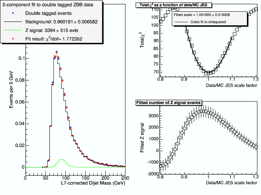
Figure 11.3.48: The $Z\to b\bar{b}$ signal extracted by CDF with 333 pb^-1 of Run II data. Left: the dijet mass of events with two $b$-tags is fit as the sum of a background template (in grey) and a signal template (in green). Top right: fit $\chi^{2}$ as a function of the $b$-JES. Bottom right: number of signal events from the fit as a function of the $b$-JES.

The resulting sample of 86,000 events contains roughly 3400 $Z$ boson decays. Their reconstructed dijet invariant mass can be fit using as a background template the mass distribution of dijet events which do not contain secondary vertices, by accounting for the bias due to the non-flat $b$-tag probability versus dijet mass using a correction function; the latter is obtained from events failing the kinematical requirements. For the $Z$ signal, 40 Monte Carlo-derived templates with a varying $b$-jet energy scale factor (JES) from 0.8 to 1.2 in steps of 0.01 are used in turn. One thus obtains the dependence of fit $\chi^{2}$ on the $b$-JES, from which a measurement of the latter can be extracted. Fig. 11.3.48 shows the results for the best fit, which corresponds to a $b$-JES of unity, with a statistical uncertainty smaller than $2\%$.

11.4 Prospects for the B-jet energy scale extraction

The largest contribution to the total uncertainty in the top quark mass determination at the Tevatron originates from the knowledge of the jet energy scale, a factor which measures the discrepancy between the effect of detector response and energy corrections in real and simulated hadronic jets. The JES can be determined from studies of photon-jet balancing[258], but modeling and selection biases limit the accuracy of the method; a determination which is mostly statistics-limited comes instead from the measurement of $W\to q\bar{q}^{\prime}$ decays in top events. With these methods, the Tevatron experiments can reach a precision close to $1\%$ on the top quark mass in Run II by reducing the JES uncertainty to a similar level.

When dealing with $b$-jets, however, one has to cope with several peculiarities of their fragmentation and decay properties, and with the different color connection of $b$-jets and light quark jets in top quark decay. All these effects have to be accurately modeled if one is to use a generic JES factor extracted from jets not containing heavy flavors to the two $b$-jets always present in a $t\bar{t}$ decay. A recent study predicts that the uncertainties in the modeling of fragmentation, decay characteristics and color flow may affect the knowledge of the $b$-JES by as little as $0.6\%$[259], but a direct determination of that quantity is of course preferable.

Due to the small cross section of production processes yielding events with a high-energy photon recoiling against a $b$-quark jet, a measurement of the $b$-JES with balancing techniques is difficult, although both D0 and CDF have recently started exploring that option.

The preliminary $Z\to b\bar{b}$ signal extracted by CDF appears to demonstrate that the data have a sufficient statistical power to allow the determination of a precise $b$-JES factor: one expects that 2 fb^-1 of data will reduce the statistical uncertainty of template fits well below $1\%$. However, systematics are a concern: given the smallness of the signal to noise ratio of the selected sample, a meaningful determination of the $b$-JES from bump fitting requires that the background shape be modeled with the utmost accuracy, especially if its most probable value occurs close to that of the $Z$ signal, as in Fig. 11.3.48.

Reducing the 20 GeV threshold on raw transverse energy of the jets, which directly affects the peak position of the background distribution, is however problematic, since low-$E_{T}$ jets suffer from subtle trigger effects which are hard to model correctly; moreover, at very low $E_{T}$ it has been shown that $c\bar{c}$ production is a sizable contribution to the SVT-triggered dataset, and its presence complicates the understanding of the $b$-tagging bias in the data.

Recent studies have shown that using large Monte Carlo samples of direct $b\bar{b}$ production processes and careful parametrizations of trigger biases it is possible to check the background shape extracted from the data as described above, and reduce the associated systematic uncertainty in the determination of the $b$-JES. CDF plans to use that additional information to finally achieve a significant measurement of the $b$-jet energy scale with $Z\to b\bar{b}$ decays, thus justifying several years of investigation of the extraction of a well-known signal.

11.5 B-jet energy resolution studies

The mass resolution of pairs of $b$-jets has been duly stressed as one of the critical factors in the search for a light Higgs boson decay at the Tevatron. While the 1999 study of the Tevatron Higgs Working Group[4] could only make the educated guess that a $\sigma_{M}/M_{bb}\sim 10\%$ relative mass resolution was attainable with a dedicated effort, the Higgs Sensitivity Working Group[132] went as far as producing some evidence that such precision was indeed reachable, by a careful use of several corrections in series, followed by the exploitation of the correlations between kinematic variables measured in $WH\to l\nu b\bar{b}$ events and the induced biases in the dijet mass measurement (see Fig. 11.5.49).

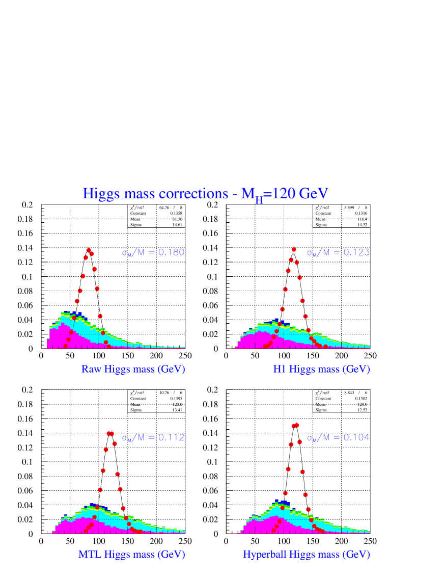
Figure 11.5.49: Dijet mass distribution for pairs of $b$-jets after different levels of jet energy corrections: raw jet energies (top left), energies corrected with the H1 algorithm (top right), then after the subsequent application of $b$-specific corrections (bottom left), and finally after the use of the hyperball algorithm, a method that corrects the dijet mass accounting for the correlation with event observables. The red points describe the behavior of $WH\to l\nu b\bar{b}$ events; the stacked histograms are Monte Carlo simulations of $W+$ jets (purple), $t\bar{t}$ production (cyan), single top production (green and yellow), and $WZ$ production (blue).

Indeed, when compared to any selection applied on the data to increase the signal to noise ratio, an algorithm that reduces the width of a resonance sitting on top of a large background has the obvious advantage of keeping intact the size of the signal. If signal significance is on the yardstick, a $20\%$ decrease of $\sigma_{M}/M_{bb}$ can be shown to have the same effect of a $20\%$ increase in collected luminosity[132].

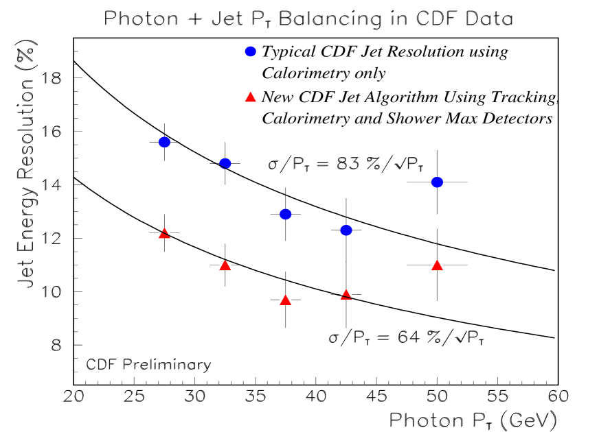
Figure 11.5.50: Jet energy resolution measured in photon+jet data as a function of photon $P_{T}$. The blue points show the resolution of the standard jet energy corrections, the red points show the results of a dedicated algorithm exploiting information from many subdetectors.

The resolution in the transverse energy of generic jets can be measured with $\gamma-jet$ events. Those events have in fact constituted the basis of CDF studies of an algorithm exploting both the tracker, the shower max detector, and the calorimeter to increase the precision of the transverse energy measurement[260]. As Fig. 11.5.50 shows, a $30\%$ improvement in the resolution of generic jets can be achieved by a combined use of the information from different subdetectors. Unfortunately, the lack of sizable samples of data containing a $b$-quark recoiling against an energetic photon prevents a data-driven study of the $b$-jet energy resolution, and a check of the effect of generic corrections applied to $b$-jets.

The development of a $b$-specific algorithm, aimed at increasing the $E_{T}$ resolution on jets containing $b$-tags, highly profits from the availability of a statistically significant sample of $Z\to b\bar{b}$ decays: one can then both check the effectiveness of any recipe and measure the resulting mass resolution.

As was noted above, $b$-jets are different from generic jets originated from light quarks or gluons in several aspects. $23\%$ of $b$-quarks decay semileptonically, and more soft leptons are yielded by the following charm quark decay; the large mass of the $b$-quark produces tracks with significant transverse momentum with respect to the jet axis; and finally, $b$-quarks have a hard fragmentation function, which may translate in an average detector response different from that of generic jets. The total effect of these peculiarities is a worse $E_{T}$ resolution for $b$-jets and a significant negative bias, mainly due to the neutrinos from semileptonic decay.

$B$-jets which are tagged by a vertex-finding algorithm are also different from an experimental point of view, since the detection of a displaced vertex allows the measurement of several ancillary characteristics: the distance between primary and secondary vertex, the total charge of tracks forming the secondary vertex, the total transverse momentum and combined mass of the charged decay tracks.

All these observable quantities can be exploited by algorithms detecting the correlation between their values and the average bias on the jet $E_{T}$ measurement. For instance, the presence of a muon in a jet is strongly correlated with the resulting calorimeter response, such that the muon $P_{T}$ can be used with success to increase the $E_{T}$ resolution. The best results are obtained when all correlations are exploited together, by finding the most probable bias in the $E_{T}$ measurement as a function of the value of all observed jet variables.

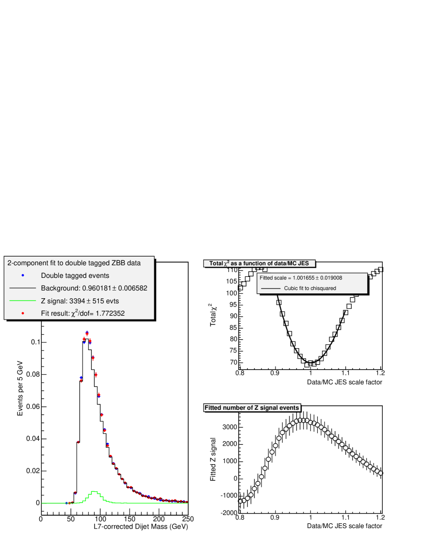
Figure 11.5.51: Relative $E_{T}$ resolution on $b$-tagged jets from a QCD $b\bar{b}$ Monte Carlo simulation, after generic jet corrections (top left, red points) and after $b$-specific jet corrections using all jet observables (bottom left, blue points). Right: a comparison of the $E_{T}$ resolution obtained with the two corrections.

Preliminary results by the CDF collaboration have determined that the $E_{T}$ resolution for $b$-jets can be improved by as much as $30\%$ from the baseline resolution yielded by the application of standard, non-$b$-specific energy corrections (see Fig. 11.5.51). Two algorithms are being developed for that purpose, and the study on the $Z\to b\bar{b}$ signal will prove their effectiveness in the near future.

12 Selected Topics in Standard Model Higgs searches using $H\rightarrow W^{+}W^{-}$ and $H\rightarrow\tau^{+}\tau^{-}$ Decays at the LHC

Contributed by: B. Mellado, W. Quayle, S. L. Wu

We study control samples for an in-situ determination of the major backgrounds to $H\rightarrow W^{+}W^{-}\rightarrow l^{+}l^{-}\nu\nu$, where a full jet veto is applied. We find that the theoretical uncertainty on the extrapolation of the QCD $W^{+}W^{-}$ background from the control sample to the signal-like region is $5\,\%$ and that the impact of the singly-resonant top background on the extrapolation from a b-tagged control sample is about 10 %. We therefore conclude that it is possible to perform a data-driven estimate of the background in the signal-like region with sufficient accuracy to achieve a $5\,\sigma$ discovery of a $160\,~{}{\rm GeV}$ Higgs with less than 2 fb^-1 of integrated luminosity. We evaluated the Next-to-Leading Order corrections to Higgs production in the analysis $H\rightarrow\tau^{+}\tau^{-}$ in association with one High $P_{T}$ jet. The ratio of NLO to LO cross-sections after the application of analysis cuts is in the range $1.5\div 1.6$ for Higgs production via gluon-gluon fusion.

12.1 Introduction

We study control samples for an in-situ determination of the major backgrounds to $H\rightarrow W^{+}W^{-}\rightarrow l^{+}l^{-}\nu\nu$, where a full jet veto is applied. We find that the theoretical uncertainty on the extrapolation of the QCD $W^{+}W^{-}$ background from the control sample to the signal-like region is $5\,\%$ and that the impact of the singly-resonant top background on the extrapolation from a b-tagged control sample is about 10 %. We therefore conclude that it is possible to perform a data-driven estimate of the background in the signal-like region with sufficient accuracy to achieve a $5\,\sigma$ discovery of a $160\,~{}{\rm GeV}$ Higgs with less than 2 fb^-1 of integrated luminosity. We evaluated the Next-to-Leading Order corrections to Higgs production in the analysis $H\rightarrow\tau^{+}\tau^{-}$ in association with one High $P_{T}$ jet. The ratio of NLO to LO cross-sections after the application of analysis cuts is in the range $1.5\div 1.6$ for Higgs production via gluon-gluon fusion.

The search for the Higgs boson called for by the Standard Model is arguably one of the most important topics in high-energy particle physics today. For the early observation of a Higgs boson of mass $115<M_{H}<135\,~{}{\rm GeV}$ the most relevant final states involve $H\rightarrow\gamma\gamma$ and $H\rightarrow\tau^{+}\tau^{-}$ [261]. For the range of masses $135<M_{H}<190\,~{}{\rm GeV}$ the most promising decay mode of the Standard Model Higgs boson is $H\rightarrow W^{+}W^{-}$ [262].

In this work, we discuss selected topics related to the search for the Standard Model Higgs boson at LHC using $H\rightarrow W^{+}W^{-}$ and $H\rightarrow\tau^{+}\tau^{-}$. In Section 12.2 we describe our Monte Carlo samples, event selection, methods for in-situ background determination for the channel $H\rightarrow W^{+}W^{-}\rightarrow l^{+}l^{-}\nu\nu$ with a full jet veto. Section 12.7 reports on studies of QCD higher order corrections to Higgs signal production in the analysis of $H\rightarrow\tau^{+}\tau^{-}$ in association with one high $P_{T}$ jet [263].

12.2 Selected Topics in $H\rightarrow W^{+}W^{-}\rightarrow l^{+}l^{-}\nu\nu$ Analysis

This Section is subdivided into four sub-sections. Sub-section 12.3 describes the Monte Carlo samples and the analysis method used in the analysis for the search of the Higgs boson with $H\rightarrow W^{+}W^{-}\rightarrow l^{+}l^{-}\nu\nu$ when applying a veto on events with high $P_{T}$ jets. We also discuss data-driven methods for the extraction of the backgrounds. In sub-sections 12.4 and 12.5 we discuss the theoretical uncertainties in the background extraction procedures. In sub-section 12.6, we perform a brief comparison of three generators for the $W^{+}W^{-}$ background for validation purposes.

12.3 Monte Carlo and Analysis Method

We consider the following signal and background processes:

• Higgs production. We model the gluon-initiated process with the generator provided in MC@NLO and normalize the cross-section for the signal to the values obtained used HIGLU [84]. The small contribution from Weak Boson Fusion (VBF) is modelled with Pythia [264, 265].

• QCD $W^{+}W^{-}$ production is modelled with the generator provided in MC@NLO version 3.1 [266, 267]. A non-negligible number of $W^{+}W^{-}$ events come from $gg\rightarrow W^{+}W^{-}$ diagrams that are not included in MC@NLO; we model this contribution using the generator documented in [268].

• $t\overline{t}$ production. The (dominant) doubly-resonant contribution is modelled with MC@NLO. To estimate the impact of the singly-resonant and non-resonant $W^{+}W^{-}bb$ contributions to the background, we perform a comparison between leading-order calculations of $pp\rightarrow W^{+}W^{-}bb$ and $pp\rightarrow t\overline{t}\rightarrow W^{+}W^{-}bb$ using MadEvent [269, 270].

• QCD $Z/\gamma$ production, with $Z\rightarrow ee/\mu\mu/\tau\tau$. We model this background with MC@NLO.

Although we do not expect detector effects to be important in this calculation, it is convenient to simulate a detector using the last fortran-based release of ATLFAST, and we apply the jet energy corrections in ATLFAST-B [271].

Cut	$gg\rightarrow H$	VBF	$t\overline{t}$	EW $WW$	$gg\rightarrow WW$	$qq\rightarrow WW$	$Z/\gamma^{*}$
Trigger and $Z$ rej.	185	25.1	7586	11.4	48.5	792	151
Hard Jet Veto	90.0	1.48	51.6	0.16	21.2	451	31.4
B Veto	89.6	1.46	37.6	0.16	21.1	449	30.8
$P_{T}^{Higgs}$	53.2	1.23	33.0	0.09	13.1	177	23.6
$M_{ll}$	42.9	1.10	7.85	0.02	6.31	65.2	22.0
$\Delta\phi_{ll}$	33.1	0.93	5.23	0.02	5.14	42.8	0.07

Table 12.3.9: Cut flows (in fb) for $M_{H}=160$ GeV in the $e\mu$ channel.

Sample	$gg\rightarrow H$	VBF	$t\overline{t}$	EW $WW$	$gg\rightarrow WW$	$qq\rightarrow WW$	$Z\rightarrow\tau\tau$
Primary	1.86	0.03	33.4	0.08	6.19	121.0	7.96
b-tagged	0.18	0.007	17.02	0.0001	0.08	1.51	1.29

Table 12.3.10: Cross-sections (in fb) in the two control samples discussed in Section 12.3 for $M_{H}=160$ GeV, summed over lepton flavor.

Our event selection consists of the following cuts:

• Trigger and Topology cuts. We require that the event has exactly two leptons with transverse momentum greater than 15 GeV in the region with $|\eta|<2.5$, and we apply a lepton identification efficiency of 90% for each lepton. The dilepton invariant mass is required to be less than 300 GeV.

• $Z$ rejection. The event is rejected if the leptons have an invariant mass between 82 and 98 GeV. We require a large missing transverse momentum $P_{T}>30$GeV, which is raised to 40 GeV if the two leptons have the same flavor. To reduce the nontrivial background from the decay $Z\rightarrow\tau\tau\rightarrow ll+P_{T}$, we calculate, using the collinear approximation, $x_{\tau}^{1}$ and $x_{\tau}^{2}$, the energy fractions carried by the visible decay products of the $\tau$ leptons, and $M_{\tau\tau}$, the invariant mass of the two $\tau$ leptons. We reject the event if $x_{\tau}^{1}>0$, $x_{\tau}^{2}>0$, and $|M_{\tau\tau}-M_{Z}|<25$GeV.

• Jet Veto. We reject the event if there are any jets with $P_{T}>30$GeV anywhere in the detector, or if it contains any b-tagged jets with $P_{T}>20$GeV and $|\eta|<2.5$. We assume a b-tagging efficiency of 60% with rejections of 10 and 100 against jets from $c$ quarks and light jets, respectively.

• Transverse momentum of the Higgs candidate. We require that $P_{T}^{Higgs}>11.1$ GeV.

In the signal-like region, we apply three more cuts: we require that the dilepton mass have $6.3<M_{ll}<64.1$ GeV, that the azimuthal opening angle between the leptons satisfy $\Delta\phi_{ll}<1.5$ radians, and that the transverse mass obey $50<M_{T}<M_{H}+10$ GeV. The cross-sections after successive cuts for a representative Higgs mass of 160 GeV in the $e\mu$ channel are shown in Table 12.3.9.

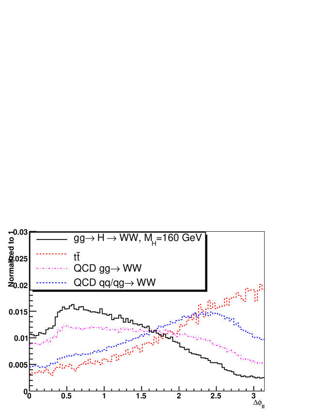
Figure 12.3.52: The distribution of the azimuthal angle (in the transverse plane) between the leptons after cuts.

We also consider two control samples:

• The primary control sample is defined the same way as the signal-like region, but with different cuts on the dilepton opening angle in the transverse plane and the dilepton invariant mass. We require $\Delta\phi_{ll}>1.5$ radians and $80<M_{ll}<300$ GeV; we remove the cut on the transverse mass.

• The b-tagged control sample cuts are the same as in the primary control sample, except that instead of applying a b-jet veto, we require that there be a b-tagged jet with $P_{T}$ between 20 GeV and 30 GeV; we also remove the lower bound on the dilepton invariant mass.

Table 12.3.10 shows the cross-sections in these two control samples. In order to make meaningful estimates of systematic errors, it is helpful to define the following three quantities:

• $\alpha_{WW}$: The ratio of the QCD $W^{+}W^{-}$ cross-section in the signal-like region over the QCD $W^{+}W^{-}$ cross-section in the primary control sample.

• $\alpha_{tt}$: The ratio of the $t\overline{t}$ cross-section in the signal-like region over the $t\overline{t}$ cross-section in the b-tagged control sample.

• $\alpha_{tt}^{WW}$: The ratio of the $t\overline{t}$ cross-section in the primary control sample over the $t\overline{t}$ cross-section in the b-tagged control sample.

With these ratios taken from Monte Carlo, we estimate the number of $t\overline{t}$ events in the signal-like region as $N_{tt}^{signal-like}=\alpha_{tt}N_{b-tagged}$ and the number of $W^{+}W^{-}$ background events in the signal-like region as

$$N_{WW}^{signal-like}=\alpha_{WW}N_{WW}^{primary}=\alpha_{WW}(N_{total}^{primary}-\alpha_{tt}^{WW}N_{b-tagged}-small~{}backgrounds)$$

where $N_{tt}^{b-tagged}$ is the number of events in the b-tagged control sample, $N_{total}^{primary}$ is the total number of events in the primary control sample, and the “$small~{}backgrounds$” consist mostly of Drell-Yan events.

12.4 Theoretical Uncertainties in the $W^{+}W^{-}$ Background

We begin with the theoretical uncertainties in the extrapolation coefficient $\alpha_{WW}$. Here, the theoretical error is dominated by the uncertainty in the normalization of the $gg\rightarrow W^{+}W^{-}$ contribution; recent studies have shown that this contribution can be in excess of 30% for the cuts used in those studies [268, 272].

We compute the the theoretical error as the sum in quadrature of the uncertainty due to the fit error in the parton density function parameterization and the uncertainty due to the choice of $Q^{2}$ scale. To estimate the parton density function (PDF) uncertainty, we have used the CTEQ6 PDF set and its error sets; using equation (3) in [273], we find that the uncertainty in $\alpha_{WW}$ is 2.8%. To assess the uncertainty due to the choice of $Q^{2}$ scale, we have varied the renormalization and factorization scales by factors of 8. We examine four choices of scale variations: Scale 1 has $Q_{ren}\rightarrow 8Q_{ren}$, $Q_{fac}\rightarrow Q_{fac}/8$; Scale 2 has $Q_{ren}\rightarrow Q_{ren}/8$, $Q_{fac}\rightarrow 8Q_{fac}$; Scale 3 has $Q_{ren}\rightarrow 8Q_{ren}$, $Q_{fac}\rightarrow 8Q_{fac}$; and Scale 4 has $Q_{ren}\rightarrow Q_{ren}/8$, $Q_{fac}\rightarrow Q_{fac}/8$. Table 12.4.11 shows the cross-sections before and after cuts in the signal-like region and primary control sample for the $gg\rightarrow W^{+}W^{-}$ and $qq\rightarrow W^{+}W^{-}$ contributions, with the central-value $Q^{2}$ scales and the four modified scale choices. The largest variation in $\alpha_{WW}$ we observe is 4.1%, and we take this to be the theoretical error due to the choice of $Q^{2}$ scale. The total theoretical uncertainty we calculate on the prediction of $\alpha_{WW}$ is therefore 5%.

	No cuts		Sig. Reg.		Cont. Samp.
Scale Choice	$gg\rightarrow WW$	$qq\rightarrow WW$	$gg$	$qq$	$gg$	$qq$	$\alpha_{WW}$
Central	487.77	11302.44	6.45	63.20	6.38	130.10	0.5103
scale1	239.93	12862.82	2.92	69.25	3.33	143.83	0.4904
scale2	1058.97	9076.86	14.5	49.03	13.46	107.44	0.5255
scale3	278.17	11189.52	3.81	65.02	3.54	131.92	0.5081
scale4	913.38	11702.80	11.1	61.81	12.66	133.51	0.4988

Table 12.4.11: Cross-sections before and after cuts for the signal-like region and the Primary control sample, with the corresponding extrapolation coefficients, using the nominal assumptions and the 4 altered scale choices.

12.5 Theoretical Uncertainties in the Top Background

We now turn our attention to the uncertainties in $\alpha_{tt}$ and $\alpha_{tt}^{WW}$. Here, the most important question to ask is how to handle single top production. A procedure for generating both $pp\rightarrow t\overline{t}$ and $pp\rightarrow Wt$ without double-counting at leading order was presented in [275], and a calculation including off-shell effects and spin correlations in the $W^{+}W^{-}bb$ system at tree level was presented in [276]. Unfortunately, we know of no event generator available at the time of this writing which also takes into account the one-loop radiative corrections to $W^{+}W^{-}bb$ production, so we will perform our uncertainty estimate at tree-level.

In addition to the $t\overline{t}$ Monte Carlo sample (from MC@NLO) that we have used in the other sections of this note, we have generated two separate $W^{+}W^{-}bb$ Monte Carlo samples using MadGraph. One includes only doubly-resonant top quark pair production, and the other includes the full $W^{+}W^{-}bb$ final state. For this generation, we have allowed the b-quarks to be generated with $P_{T}$ as low as 1 GeV, and with pseudorapidity as high as 100. One would expect a disproportionately large contribution from the region where one b-quark is soft or forward, and we therefore feel it is likely that the single-top contribution is overestimated in our nonresonant $W^{+}W^{-}bb$ Monte Carlo. This is exactly what we want if we are to prove that our analysis is robust. We have applied the cuts for the signal-like region and both of the control regions to these two Monte Carlo samples to assess the importance of single-top production in this analysis.

Process	Signal-like	Cont. Samp.	b-tagged	$\alpha_{tt}$	$\alpha_{tt}^{WW}$
$W^{+}W^{-}bb$	13.34	109.41	47.13	0.2829	2.3211
$tt\rightarrow W^{+}W^{-}bb$	9.80	80.77	37.72	0.2599	2.1413

Table 12.5.12: Cross-sections (in fb) and extrapolation coefficients for the $t\overline{t}$ background for various masses, using MadGraph to model the $W^{+}W^{-}bb$ background.

Table 12.5.12 shows the $W^{+}W^{-}bb$ background cross-sections in the signal-like region, the primary control sample, and the b-tagged control sample obtained with the leading-order doubly-resonant $t\overline{t}$ and inclusive $W^{+}W^{-}bb$ samples. We note that although the difference in the absolute cross-section given by the two samples is approximately 30%, the corresponding differences in the predictions of $\alpha_{tt}$ and $\alpha_{tt}^{WW}$ are only about 9%. It is worth noting that this figure is only a general guideline, since the exact values of $\alpha_{tt}$ and $\alpha_{tt}^{WW}$ are strongly dependent on the particulars of the b-tagging algorithm used. Our intent in this section is only to give a rough idea of what the theoretical uncertainty on the extrapolation from a b-tagged sample to a b-vetoed sample should be. In practice, this uncertainty should be addressed in detail using full detector simulation by any experimenter performing a $H\rightarrow W^{+}W^{-}$ search like the one outlined here.

12.6 Comparison of MC@NLO, Alpgen, and Sherpa

In this subsection, we check the agreement among the predictions of the QCD $W^{+}W^{-}$ background given by MC@NLO and by tree-level jet-parton matching algorithms like the ones in Sherpa and Alpgen. We begin with a few general comments about the generators under study. In this sub-section we ignore the process $gg\rightarrow W^{+}W^{-}$.

• All three generators ignore the contribution from gluon-initiated diagrams that contain a quark box. This contribution is not negligible; in practice, we treat the gluon-initiated contribution as a separate process modelled with a separate generator.

• The matrix element calculations in MC@NLO and Alpgen were programmed by hand by their respective authors, while Sherpa uses an automated matrix element generator to write code to compute the (tree-level) matrix elements relevant to a particular process. There are therefore some differences regarding which Feynman diagrams are included in the two calculations. In the case of this analysis, where we are concerned with the production of W pairs which decay leptonically, Sherpa includes the contribution from diagrams where two $Z$ bosons are produced, with one $Z$ decaying to leptons and the other to neutrinos. This leads to a spike in the dilepton invariant mass distribution in events with same-flavor leptons; this feature does not appear to be present in MC@NLO and Alpgen. For this reason, we will consider only events with one electron and one muon in this section.

• MC@NLO includes the contribution from loop diagrams in its calculation; Sherpa and Alpgen rely instead on jet-parton matching schemes like the one discussed in [277].

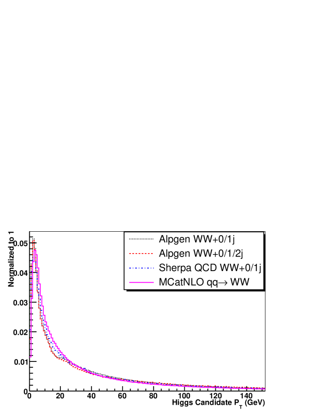
Figure 12.6.53: The transverse momentum of the Higgs candidate in QCD $W$ pair production as given by Alpgen, Sherpa, and MC@NLO. There is a small shift in the location of the peak, but the difference is not dramatic at all.

It is worthwhile to point out that although the treatment of soft hadronic physics in Alpgen, Sherpa, and MC@NLO are all quite different, the result is nevertheless similar for the three generators. Figure 12.6.53 shows the distribution of the transverse momentum of the Higgs candidate (in the $e-\mu$ channel) given by Alpgen, Sherpa, and MC@NLO for the QCD $W^{+}W^{-}$ background. Although a detailed study of the errors on these distributions is beyond the scope of this work, we feel that the similarity among all three generators is encouraging. We note that the Alpgen and Sherpa samples predict a slightly lower cross-section for events with Higgs candidate $P_{T}$ between roughly 10 and 25 GeV. This is no doubt an artifact of the jet-parton matching method, and we expect that the behavior of this region could be tuned by tuning the matching parameters in the respective generators (although such a tuning is not necessary for our analysis).

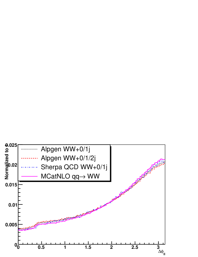
Figure 12.6.54: The distribution of the azimuthal angle between the leptons (in the $e-\mu$ channel) in QCD $W$ pair production as given by Alpgen, Sherpa and MC@NLO.

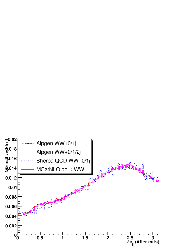
Figure 12.6.55: The distribution of the azimuthal angle between the leptons (in the $e-\mu$ channel) in QCD $W$ pair production as given by Alpgen, Sherpa and MC@NLO. This figure plots the distributions after all cuts except the cuts on $M_{ll}$, $\Delta\phi_{ll}$, and $M_{T}$.

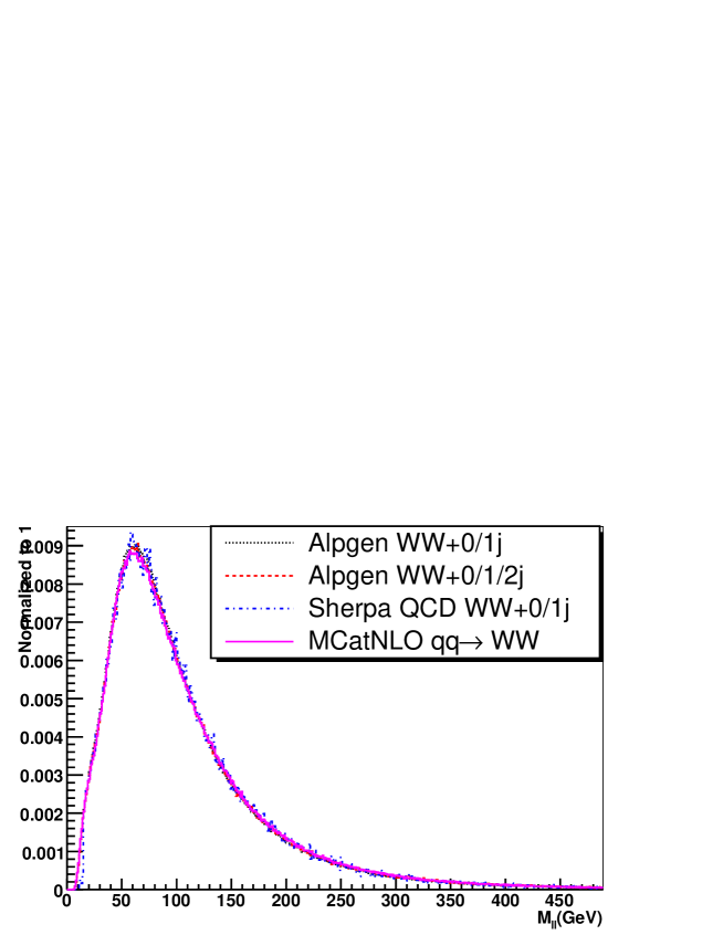
Figure 12.6.56: The distribution of the dilepton invariant mass (in the $e-\mu$ channel) in QCD $W$ pair production as given by Alpgen, Sherpa and MC@NLO.

It is also worthwhile to compare the predictions of variables related to spin correlations in the $W^{+}W^{-}$ system, as these correlations are crucially important for the analysis. Figure 12.6.54 shows the distribution of the azimuthal angle between the leptons (in the $e-\mu$ channel) before the cuts in the next section; there is a slight difference in the shape of these inclusive distributions. The discrepancy is not serious at all; we believe it is a kinematic effect caused by the depletion in events with Higgs $P_{T}$ between 10 and 25 GeV mentioned in the previous paragraph. Figure 12.6.55 shows the distribution of the dilepton opening angle in the transverse plane after all but the last three cuts of Section 12.3 have been applied; there is good agreement for this distribution among the various generators. Figure 12.6.56 shows the dilepton invariant mass for events with one electron and one muon (before the cuts of the analysis are applied); it is clear from the figure that the distribution of this variable is also very similar in all three generators.

12.7 QCD NLO Corrections for Higgs Production in $H\rightarrow\tau^{+}\tau^{-}$ in Association with One High $P_{T}$ Jet

In a recent publication it was demonstrated that the search for the Higgs boson using the $H\rightarrow\tau^{+}\tau^{-}$ decay in association with one high $P_{T}$ jet is a promising discovery channel at the LHC [263]. Next-to-Leading order corrections (NLO) were not evaluated for the final state considered in [263].

There are two main requirements in the analysis, which are instrumental in achieving a good signal-to-background ratio: the application of a large cut on the $P_{T}$ of the Higgs candidate ($P_{TH}>100\,~{}{\rm GeV}$) and the requirement that the invariant mass of the Higgs candidate and the leading jet in the event be very large ($M_{HJ}>700\,~{}{\rm GeV}$). In addition to the two cuts just mentioned it was necessary to require that there be no additional hard jets (hadron level $P_{T}>20\,~{}{\rm GeV}$) in the central region of the detector ($\left|\eta\right|<2)$. The latter is introduced to suppress the $t\overline{t}$ background.

It is meaningful to evaluate QCD higher order corrections to the signal process after the application of the cuts mentioned above. Apart from a chance in the overall normalization, the impact of extra jets in the final state on the analysis is not expected to be trivial.

In order to evaluate QCD Next-to-Leading corrections, we use the MCFM program [278]. This package enables the user to apply cuts at the parton level. Next-to-Leading Order matrix elements to Higgs production in association with one jet are available. In this calculation the infinite top mass approximation is used. In addition, NLO matrix elements for Higgs production via weak boson fusion are also available within MCFM.

Figure 12.7.57 shows the Higgs $P_{T}$ (plots on the left) and the invariant mass of the Higgs and the leading jet (plots on the right) for Higgs produced via gluon-gluon fusion. The upper plots in Figure 12.7.57 show the distributions to Leading Order (LO, solid lines) and to NLO (dashed lines). The lower plots in Figure 12.7.57 show the ratio of the NLO to the LO cross-sections.

Figure 12.7.57 illustrates that the QCD NLO corrections to the signal produced via gluon-gluon fusion in the region of the phase space where the Higgs boson will be searched for are large. The size of the NLO correction is larger than the correction before the application of cuts on the Higgs $P_{T}$ and $M_{HJ}$. The perturbative analysis shows that the NLO correction grows with $M_{HJ}$. This can be understood qualitatively: for large values of $M_{HJ}$ a large $P_{T}$ extra parton is likely to be present in the final state, providing extra transverse momentum to the system made by the Higgs and the leading jet and indirectly enhancing its invariant mass.

Figure 12.7.57: Higgs $P_{T}$ (plots on the left) and the invariant mass of the Higgs and the leading jet (plots on the right) for Higgs produced via gluon-gluon fusion. The upper plots show the distributions to Leading Order (solid lines) and to Next-to-Leading Order (dashed lines). The lower plots show the ratio of the Next-to-Leading Order to the Leading Order cross-sections. The package MCFM was used to evaluate the cross-sections. Cross-sections are given in fb per bin.

As pointed out above in this Section, the application of a veto on extra hadronic activity is important for the suppression of the $t\overline{t}$ production. It is necessary to evaluate the QCD NLO corrections after the addition of this jet veto. Plots in Figure 12.7.58 show the same distributions as in Figure 12.7.57 after the application of a veto on events with an extra parton with $P_{T}>30\,~{}{\rm GeV}$ and $\left|\eta\right|<2$. The plots on the left illustrate that after the application of a veto on extra high $P_{T}$ partons changes size of the NLO corrections takes place. The ratio of NLO to LO cross-sections decreases with the Higgs $P_{T}$ for $P_{T}>50\,~{}{\rm GeV}$. After the application of the veto the ratio of the NLO to LO cross-sections becomes flat as a function of $M_{HJ}$ instead of increasing, as illustrated in Figure 12.7.57.

Figure 12.7.58: Same as Figure 12.7.57 after requiring a veto on an additional parton with $P_{T}>30\,~{}{\rm GeV}$ and $\left|\eta\right|<2$.

After the application of the cuts described above in this section the ratio of the NLO to the LO cross-sections remains large, in the range $1.5\div 1.6$.

A similar analysis was performed with the Higgs production via weak boson fusion. Before the application of a jet veto the impact of QCD NLO corrections on the Higgs $P_{T}$ and $M_{HJ}$ distributions is mild and have little impact on the sensitivity of the channel.

12.8 Summary

We have proposed a method to estimate the normalization of the dominant backgrounds in the $H\rightarrow W^{+}W^{-}\rightarrow l^{+}l^{-}\nu\nu$ channel using two control samples in the data, one b-tagged, and the other b-vetoed; in our approach, the systematic errors must be given in terms of the ratios $\alpha_{WW}$, $\alpha_{tt}$, and $\alpha_{tt}^{WW}$. We have computed the theoretical uncertainty on $\alpha_{WW}$; the result is 5%. We have shown that, for a b-tagging algorithm operating only on jets with $P_{T}>20$ GeV and $|\eta|<2.5$, such that $\epsilon_{b}=60$% and the rejections against light quarks and c-quarks are 100 and 10 respectively, the effect of singly-resonant and non-resonant $W^{+}W^{-}bb$ diagrams is less than 10% on $\alpha_{tt}$ and $\alpha_{tt}^{WW}$. A study using these uncertainties and this background extraction technique is in progress; the preliminary result is that a Higgs discovery at $M_{H}=160$ GeV would require less than 2 fb^-1 of integrated luminosity [279]. However, final calculations of the uncertainties on these last two extrapolation coefficients, as well as final results on the overall sensitivity of the search we have presented here, must be computed within the context of the LHC experiments.

We have evaluated the QCD NLO corrections for signal in the Higgs search with $H\rightarrow\tau^{+}\tau^{-}$ in association with one high $P_{T}$ jet. The ratio of the NLO to LO cross-sections for Higgs production via gluon-gluon fusion is well above $2$ for Higgs $P_{T}>50\,~{}{\rm GeV}$ and increases with $M_{HJ}$. The ratio drops substantially with the application of a veto on events with an extra parton with $P_{T}>30\,~{}{\rm GeV}$ and $\left|\eta\right|<2$. After the application of analysis cuts the ratio of the NLO to LO cross-sections for Higgs signal produced via gluon-gluon fusion is in the range $1.5\div 1.6$.

12.9 Acknowledgement

The authors are grateful to J. Campbell, N. Kauer and S. Frixione. We also would like to thank the organizers and the convenors of the Higgs working group of the very successful TEV4LHC workshop. This work was supported in part by the United States Department of Energy through Grant No. DE-FG0295-ER40896.

13 An invisibly decaying Higgs at Tevatron and LHC

Contributed by: H. Davoudiasl, T. Han, H.E. Logan

The Higgs particle is the only missing part of the highly successful Standard Model (SM) of particle physics. The current experimental data from direct searches [131] and electroweak precision measurements [280, 281, 282] point to a Higgs mass in the range $114\mathrm{\ Ge\kern-1.00006ptV}<m_{h}\lesssim 250\mathrm{\ Ge\kern-1.00006ptV}$. Thus, if the Higgs exists the Tevatron might detect it in the next several years and the LHC is expected to discover it.

Most analyses assume that the Higgs will predominantly decay into detectable SM fields. However, this may not be a good assumption if there are new weakly interacting particles with mass less than half the Higgs mass that couple to the Higgs with ${\cal O}(1)$ strength. In this case, if $m_{h}<160\mathrm{\ Ge\kern-1.00006ptV}$ $\simeq 2\,m_{W}$ so that the Higgs partial width into SM particles is very small, the Higgs will decay predominantly into the new weakly interacting particles. In particular, if these new weakly interacting particles are neutral and stable, the Higgs will decay invisibly. There are many models in which this situation is realized, such as the Minimal Supersymmetric Standard Model (MSSM, with Higgs decays to lightest neutralinos), models with extra dimensions (with Higgs decays to Kaluza-Klein neutrinos [283]), and Majoron models [284, 285]. An invisible Higgs is also quite generic in minimal models of dark matter containing a stable singlet scalar [286, 287, 288]. The combined LEP experimental bound on the mass of an invisibly-decaying Higgs boson is 114.4$\mathrm{\ Ge\kern-1.00006ptV}$ at 95$\%$ confidence level [289].

In this work, we study the discovery potential for the invisible Higgs $h_{inv}$ at the LHC and the Tevatron in the channels $Z+h_{\mathrm{inv}}$ and $h_{\mathrm{inv}}+jj$ in Weak Boson Fusion (WBF). There have been a number of similar studies in the past [290, 291, 292, 293, 294, 295, 296, 297, 298]. We also examine the prospects for determining the mass of the invisible Higgs from production cross sections at the LHC. We show that the $Z+h_{\mathrm{inv}}$ channel gives a surprisingly good handle on the Higgs mass given 100 fb^-1 of integrated luminosity. We also show how the $Z+h_{\mathrm{inv}}$ and WBF channels can be combined at the LHC to remove model assumptions from the Higgs mass extraction. A more detailed account of this study can be found in Ref. [299].

13.1 Production of $h_{\mathrm{inv}}$ via WBF at the Tevatron

WBF production of the invisible Higgs was studied for the LHC in Ref. [295], which showed that WBF can provide significant signals for invisible Higgs discovery, even at low luminosity. Here, we will use their approach to show that WBF contributes significantly to the observation of $h_{\mathrm{inv}}$ at the Tevatron. Even though a 3$\sigma$ observation of a 120$\mathrm{\ Ge\kern-1.00006ptV}$ $h_{\mathrm{inv}}$ in any single channel at the Tevatron is not possible with less than 12 fb^-1 per detector, one can enhance the significance of the signal by combining data from various channels. At the Tevatron, an important production mode is $Z+h_{\mathrm{inv}}$ [294] and yields a somewhat larger significance than the WBF channel that we study. Combining these two channels and data from two Tevatron detectors, we show that a 3$\sigma$ observation of $h_{\mathrm{inv}}$ with $m_{h}=120\mathrm{\ Ge\kern-1.00006ptV}$ can be obtained with 7 fb^-1 of integrated luminosity per detector.

At the LHC, the kinematic requirements for suppressing the backgrounds rely on the large energy and rapidity of the forward tagging jets characteristic of WBF at the LHC, together with the large rapidity coverage of the LHC detectors. Despite the more limited kinematic range and rapidity coverage at the Tevatron, we show that the WBF production mode will indeed have a significant impact on the prospects for the observation of $h_{\mathrm{inv}}$ at the Tevatron, before data from the LHC becomes available.

The signal here is $P_{T}+2j$. A large background comes from $Z(\to\nu{\bar{\nu}})+2j$ with the jets produced via QCD. A smaller, but less reducible, background comes from $Z(\to\nu{\bar{\nu}})+2j$ in which the $Z$ is produced by WBF and the jets have kinematics similar to that of the signal. In addition, there are backgrounds from $W(\to\ell\nu)+2j$, in which the lepton from the $W$ decay is missed, and QCD backgrounds with fake $P_{T}$ from missed jets in multi-jet events and jet energy mismeasurements in di-jet events.

We generate the signal, $h_{\mathrm{inv}}+2j$, the QCD and electroweak backgrounds with $Z(\to\nu\bar{\nu})+2j$, and the QCD background with $W(\to\ell\nu)+2j$ for the Tevatron using Madgraph [269, 242]. We start with the following “minimal cuts”:

$$p_{T}(j)>10\mathrm{\ Ge\kern-1.00006ptV},\qquad\qquad|\eta(j)|<3.0,\qquad\qquad\Delta R(jj)>0.4,\qquad\qquad P_{T}>90\mathrm{\ Ge\kern-1.00006ptV}.$$ (13.1.83)

The $P_{T}>90\mathrm{\ Ge\kern-1.00006ptV}$ requirement provides a trigger. We take the calorimeter pseudo-rapidity coverage from, e.g., Ref. [300].

We impose “WBF cuts”: we require that the two jets reconstruct to a large invariant mass,

$$m_{jj}>320,\ 340,\ 360,\ 400\mathrm{\ Ge\kern-1.00006ptV},$$ (13.1.84)

and are separated by a large rapidity gap,

$$\Delta\eta_{jj}>2.8.$$ (13.1.85)

These two cuts eliminate most of the QCD $Z+2j$ and $W+2j$ backgrounds, in which the jets tend to be softer and have a smaller rapidity gap, while preserving a significant fraction of the WBF signal.

To reduce the $W+2j$ background further, we apply a lepton veto. We veto events that contain an isolated electron with [301]

$$p_{T}(\ell)>8\mathrm{\ Ge\kern-1.00006ptV},\qquad\qquad|\eta(\ell)|<3.0.$$ (13.1.86)

For simplicity, we apply the same veto to $W$ decays to muons or taus. Loosening the veto requirements to $p_{T}(\ell)>10\mathrm{\ Ge\kern-1.00006ptV},|\eta(\ell)|<2.0$ increases the $W+2j$ background by about a factor of two.

Background can also come from QCD multi-jet events with fake $P_{T}$ due to mismeasurement of jets and jet activity escaping down the beampipe. We follow the techniques of a CDF study of $P_{T}+2j$ [302] to deal with this background. Please see Ref.[299] for more details.

In Table 13.1.13 we show results for signal and background cross sections for the $m_{jj}$ cuts given in Eq. (13.1.84). In Table 13.1.14 we show the resulting signal-to-background ratio and significance for 10 fb^-1.

$m_{jj}$ cut	S($h_{\mathrm{inv}}+2j$)	B($Z+2j$,QCD)	B($Z+2j$,EW)	B($W+2j$,QCD)
320$\mathrm{\ Ge\kern-1.00006ptV}$	4.1 fb	55 fb	1.7 fb	7 fb
340$\mathrm{\ Ge\kern-1.00006ptV}$	3.6 fb	43 fb	1.6 fb	5 fb
360$\mathrm{\ Ge\kern-1.00006ptV}$	3.2 fb	34 fb	1.4 fb	5 fb
400$\mathrm{\ Ge\kern-1.00006ptV}$	2.4 fb	21 fb	1.2 fb	2 fb

Table 13.1.13: Signal and background cross sections for $h_{\mathrm{inv}}+2j$ at Tevatron Run 2, for $m_{h}=120\mathrm{\ Ge\kern-1.00006ptV}$. The statistical uncertainty on B($Z+2j$,QCD) after cuts is roughly 10% due to our limited Monte Carlo sample. There is an additional background from QCD with fake $P_{T}$ which is taken from Ref. [302] to be 5 fb; this represents a conservative overestimate of the fake $P_{T}$ background.

$m_{jj}$ cut	S (10 fb-1)	S/B	S/$\sqrt{\rm B}$ (10 fb-1)
320$\mathrm{\ Ge\kern-1.00006ptV}$	41 evts	0.060	1.6
340$\mathrm{\ Ge\kern-1.00006ptV}$	36 evts	0.066	1.5
360$\mathrm{\ Ge\kern-1.00006ptV}$	32 evts	0.070	1.5
400$\mathrm{\ Ge\kern-1.00006ptV}$	24 evts	0.082	1.4

Table 13.1.14: Number of signal events, signal-to-background ratio, and significance for $h_{\mathrm{inv}}+2j$ at Tevatron Run 2, for $m_{h}=120\mathrm{\ Ge\kern-1.00006ptV}$. We include the background from QCD with fake $P_{T}$ of 5 fb [302] in S/B and S/$\sqrt{\rm B}$.

We find a signal significance of about 1.6$\sigma$ with 10 fb^-1 of luminosity at one Tevatron detector. This significance is not much less than that found in Ref. [294] for $Z+h_{\mathrm{inv}}$ at the Tevatron, namely $1.9\sigma$ with 10 fb^-1 for $m_{h}=120\mathrm{\ Ge\kern-1.00006ptV}$. Combining data from both Tevatron detectors, a $3\sigma$ observation would require at least 12 fb^-1 in the $Z+h_{\mathrm{inv}}$ channel, or 18 fb^-1 in the WBF channel. However, by combining these two channels, we find that a 3$\sigma$ observation of $h_{\mathrm{inv}}$ is possible with 7 fb^-1 per detector, if the background can be determined to better than 10%. Thus, WBF provides an important second channel that brings an observation of $h_{\mathrm{inv}}$ into the realm of possibility at the Tevatron before the results of the LHC become available. Here, we note that there may be other production channels, such as $gg\to h_{inv}jj$, that could contribute to the signal, even after the WBF cuts we have outlined. However, this could only enhance $h_{inv}$ production, making our results for the WBF channel a lower bound on the number of signal events.

In Refs. [295, 303], it is claimed that vetoing additional soft jets in the central region improves the signal-to-background ratio by a factor of three at the LHC. If a similar background reduction could be achieved at the Tevatron, the prospects for $h_{\mathrm{inv}}$ observation in the WBF channel would improve considerably: a $3\sigma$ observation in the WBF channel alone would then be possible with 6 fb^-1 per detector, with a signal-to-background ratio close to 1/5. Further discussion of background reduction is presented in Ref. [299]. We emphasize that we have not applied a central jet veto to obtain the results in Tables 13.1.13 and 13.1.14.

13.2 Associated $Z+h_{\mathrm{inv}}$ Production at the LHC

Discovery of the Higgs in the $Z+h_{\mathrm{inv}}$ channel was studied for the LHC in Refs. [293, 296]. This channel was also analyzed for the Tevatron in Ref. [294]. In Ref. [293], the $Z+$jet background at the LHC was found to diminish the significance of the signal considerably, and the electroweak backgrounds coming from $WW$ and $ZW$ final states were ignored. We update and refine the analysis of Ref. [293] by taking into account sources of background not included in that study and considering a wider acceptance range for the leptons. We show that, with the kinematic acceptance and the cuts we adopt, the prospects for the discovery of the invisible Higgs in $Z+h_{\mathrm{inv}}$ at the LHC are brighter than presented in Ref. [293], even with the $WW$ and $ZW$ backgrounds included. Our results are consistent with those of Ref. [296].

We consider the production process

$$p\,p\to Z(\to\ell^{+}\ell^{-})+h_{\mathrm{inv}}\,\,;\qquad\ell=e,\mu,$$ (13.2.87)

at the LHC. We assume that the Higgs decays 100% of the time to invisible final states, and that the production cross section is the same as in the SM. Our results can be easily scaled for other invisible branching fractions or non-SM production cross sections. The signal rate is simply scaled by the production rate and invisible branching fraction:

$$S=S_{0}\frac{\sigma}{\sigma_{SM}}\frac{{\rm BR}_{inv}}{1},$$ (13.2.88)

where $S_{0}$ is the signal rate from our studies, $\sigma/\sigma_{SM}$ is the ratio of the nonstandard production cross section to that of the SM Higgs, and BR_inv is the invisible branching fraction. Assuming that the SM is the only source of background, the luminosity required for a given signal significance then scales like

$$\mathcal{L}=\mathcal{L}_{0}\left[\frac{\sigma}{\sigma_{SM}}\frac{{\rm BR}_{inv}}{1}\right]^{-2},$$ (13.2.89)

where $\mathcal{L}_{0}$ is the luminosity required for a given significance found in our studies.

Signal for $h_{\mathrm{inv}}$

As the signal is $\ell^{+}\ell^{-}P_{T}$, the most significant sources of background are

$$Z(\to\ell^{+}\ell^{-})Z(\to\nu{\bar{\nu}}),\qquad W^{+}(\to\ell^{+}\nu)W^{-}(\to\ell^{-}{\bar{\nu}}),\qquad Z(\to\ell^{+}\ell^{-})W(\to\ell\nu),$$ (13.2.90)

(with the lepton from the $W$ decay in $ZW$ missed) and $Z+{\rm jets}$ final states with fake $P_{T}$ [293, 294]. We simulate the signal and the first three backgrounds for the LHC using Madgraph [269, 242].

We start with the following “minimal cuts”:

$$p_{T}(\ell^{\pm})>10\mathrm{\ Ge\kern-1.00006ptV},\qquad\qquad|\eta(\ell^{\pm})|<2.5,\qquad\qquad\Delta R(\ell^{+}\ell^{-})>0.4,$$ (13.2.91)

where $\eta$ denotes pseudo-rapidity and $\Delta R$ is the separation between the two particles in the detector, $\Delta R\equiv\sqrt{(\Delta\eta)^{2}+(\Delta\phi)^{2}}$; $\phi$ is the azimuthal angle. The electromagnetic calorimeter at both ATLAS [304] and CMS [305] covers the range $|\eta|<3$; however, the electron trigger covers only $|\eta|<2.5$ (2.6) at ATLAS (CMS). The pseudo-rapidity acceptance for dielectrons could be expanded by requiring only one electron within $|\eta|<2.5$ and the other within $|\eta|<3$. Meanwhile, the muon trigger covers $|\eta|<2.2$ (2.1) at ATLAS (CMS), with muon identification and momentum measurement out to $|\eta|<2.4$. We require $|\eta(\ell^{\pm})|<2.5$ for both leptons, so that the larger acceptance for dielectron events compensates the smaller acceptance for dimuon events.

Because we will cut on the invariant mass of the dilepton pair to keep only events in which the dileptons reconstruct to the $Z$ mass, we imitate the effects of LHC detector resolution by smearing the electron momenta according to

$$\Delta E/E={0.1\over\sqrt{E(\mathrm{\ Ge\kern-1.00006ptV})}}\oplus 0.5\%,$$ (13.2.92)

with the two contributions added in quadrature. This smearing has a negligible effect on our results. We have thus applied the same smearing to the final state with muons.

The $WW$ background can be largely eliminated by requiring that the $\ell^{+}\ell^{-}$ invariant mass $m_{\ell^{+}\ell^{-}}$ is close to $m_{Z}$:

$$|m_{\ell^{+}\ell^{-}}-m_{Z}|<10\mathrm{\ Ge\kern-1.00006ptV}.$$ (13.2.93)

Also, the $\ell^{+}$ and $\ell^{-}$ from two different parent $W$ bosons tend to be more back-to-back than the leptons in the signal. We therefore impose an azimuthal angle cut on the lepton pair,

$$\Delta\phi_{\ell^{+}\ell^{-}}<2.5\ \ {\rm or}\ \ 143^{\circ}.$$ (13.2.94)

This cut also eliminates Drell-Yan backgrounds with fake $P_{T}$ caused by mismeasurement of the lepton energies.

Our third cut is on $P_{T}$. The number of $\ell^{+}\ell^{-}P_{T}$ signal events typically falls more slowly with $P_{T}$ than those of the $ZZ$ or $WW$ backgrounds, as shown in Fig. 13.2.59.

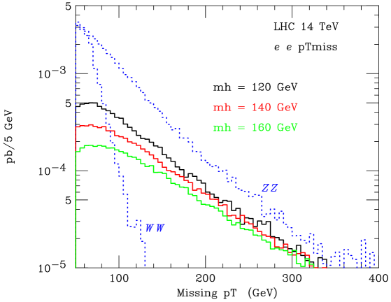
Figure 13.2.59: Missing $p_{T}$ distribution for $Z(\to e^{+}e^{-})+h_{\mathrm{inv}}$ signal (solid lines, with $m_{h}=120$, 140 and 160$\mathrm{\ Ge\kern-1.00006ptV}$ top to bottom) and backgrounds from $WW$ and $ZZ$ (dotted lines) at the LHC, after applying the cuts in Eqs. (13.2.91), (13.2.93) and (13.2.94).

The final state $Z(\to\ell^{+}\ell^{-})W(\to\ell\nu)$, where the lepton from the $W$ decay is missed, can be a potential background. However, the probability of missing the lepton from the $W$ decay is small given the kinematic coverage at the LHC. To reduce this background, we veto events with a third isolated electron with

$$p_{T}>10\mathrm{\ Ge\kern-1.00006ptV},\qquad\qquad|\eta|<3.0.$$ (13.2.95)

For simplicity, we apply the same veto to $W$ decays to muons or taus. This veto reduces the $Z+W$ background to the level of 5–10 fb, so that it has little effect on the significance of the signal.

We also include the background from $Z+{\rm jets}$ with fake $P_{T}$. As shown in Ref. [293], events of the type $Z+$jets can constitute a significant background due to jet energy mismeasurements resulting in fake $P_{T}$, or when one or more jets are emitted outside the fiducial region of the detector and are therefore missed. The majority of those events can be eliminated by applying a jet veto, but those in which the jet(s) are soft and/or escape down the beampipe can fake $Z+P_{T}$ events. A simulation of the latter requires simulating the detector effects, which is beyond the scope of our analysis. Instead, as explained in Ref. [299], we adopt the results for this background from Ref. [293].

At this point, we note that there are other potentially large sources of background that need to be addressed [294]. The background events from $Z^{*}\to\tau^{+}\tau^{-}\to\ell^{+}\ell^{-}P_{T}$ are efficiently suppressed by our $Z$-mass cut on $m_{\ell^{+}\ell^{-}}$, the $P_{T}$ cut, and the cut on $\Delta\phi_{\ell^{+}\ell^{-}}$ that requires that the leptons are not back-to-back. This can be seen from Table 2 in Ref. [296], where it is shown that, after cuts similar to those we use, the resulting background from a single $Z$ is basically absent for the $ZH$ production channel. The same conlcusion is reached for the $W+{\rm jet}$ background in the $ZH$ channel, in Table 2 of Ref. [296]. Hence, fake events from $W(\to\ell\nu)+$jet, where the jet is misidentified as a lepton of the appropriate charge and flavor, are also ignored in our analysis.

Our results for the background and signal cross sections are tabulated in Table 13.2.15. The corresponding signal to background ratio, $S/B$, and significance, $S/\sqrt{B}$, are tabulated in Table 13.2.16. We see from Table 13.2.16 that a $>5\sigma$ discovery can be obtained for $m_{h}=120\mathrm{\ Ge\kern-1.00006ptV}$ with 10 fb^-1 of integrated luminosity, even with our conservative estimate for the $Z+$jets background for $P_{T}>75\mathrm{\ Ge\kern-1.00006ptV}$. With 30 fb^-1, discovery can be pushed out to $m_{h}=160\mathrm{\ Ge\kern-1.00006ptV}$.

					S($Z+h_{\mathrm{inv}}$)
$P_{T}$ cut	B($ZZ$)	B($WW$)	B($ZW$)	B($Z+j)^{*}$	$m_{h}=120$	140	160$\mathrm{\ Ge\kern-1.00006ptV}$
65$\mathrm{\ Ge\kern-1.00006ptV}$	48.0 fb	10.6 fb	10.2 fb	22 fb	14.8 fb	10.8 fb	7.9 fb
75$\mathrm{\ Ge\kern-1.00006ptV}$	38.5 fb	4.3 fb	7.4 fb	9 fb	12.8 fb	9.4 fb	7.0 fb
85$\mathrm{\ Ge\kern-1.00006ptV}$	30.9 fb	1.8 fb	5.5 fb		11.1 fb	8.3 fb	6.3 fb
100$\mathrm{\ Ge\kern-1.00006ptV}$	22.1 fb	0.6 fb	3.6 fb		8.7 fb	6.8 fb	5.3 fb

Table 13.2.15: Background and signal cross sections for associated $Z(\to\ell^{+}\ell^{-})+h_{\mathrm{inv}}$ production at the LHC, combining the $ee$ and $\mu\mu$ channels. ^∗Estimated from Ref. [293] (see text for details).

	$m_{h}=120\mathrm{\ Ge\kern-1.00006ptV}$			$m_{h}=140\mathrm{\ Ge\kern-1.00006ptV}$	$m_{h}=160\mathrm{\ Ge\kern-1.00006ptV}$
$P_{T}$ cut	S/B	S/$\sqrt{\rm B}$ (10 fb-1)	S/$\sqrt{\rm B}$ (30 fb-1)	S/$\sqrt{\rm B}$ (30 fb-1)	S/$\sqrt{\rm B}$ (30 fb-1)
65$\mathrm{\ Ge\kern-1.00006ptV}$	0.22 (0.16)	5.6 (4.9)	9.8 (8.5)	7.1 (6.2)	5.2 (4.5)
75$\mathrm{\ Ge\kern-1.00006ptV}$	0.25 (0.22)	5.7 (5.3)	9.9 (9.1)	7.3 (6.7)	5.4 (5.0)
85$\mathrm{\ Ge\kern-1.00006ptV}$	0.29	5.7	9.8	7.4	5.6
100$\mathrm{\ Ge\kern-1.00006ptV}$	0.33	5.4	9.3	7.3	5.7

Table 13.2.16: Signal significance for associated $Z(\to\ell^{+}\ell^{-})+h_{\mathrm{inv}}$ production at the LHC, combining the $ee$ and $\mu\mu$ channels. The numbers in the parentheses include the estimated $Z+$jets background discussed in the text.

The $Z+h_{\mathrm{inv}}$ channel can thus be used at the LHC for $m_{h}\lesssim 160\mathrm{\ Ge\kern-1.00006ptV}$ to supplement the WBF channel [295], which has higher significance. WBF production of $h_{\mathrm{inv}}$ at the LHC was studied in Ref. [295], which concluded that with only 10 fb^-1 of integrated luminosity, $h_{\mathrm{inv}}$ can be detected at the $\geq 5\sigma$ level up to $m_{h}\simeq 480\mathrm{\ Ge\kern-1.00006ptV}$. They also showed that the invisible branching fraction of a 120$\mathrm{\ Ge\kern-1.00006ptV}$ Higgs can be constrained at the 95% confidence level to be less than $13\%$ if no signal is seen in the WBF$\to h_{\mathrm{inv}}$ channel, again with 10 fb^-1. However, we would like to emphasize that the $P_{T}$ measurements in the process $\ell^{+}\ell^{-}P_{T}$ that we studied here are largely determined by $p_{T}(\ell\ell)$, and the distribution will suffer much less from systematic uncertainties compared to the WBF where $P_{T}$ is determined mainly from the forward jets.

Higgs boson mass

The $Z+h_{\mathrm{inv}}$ channel may also provide an interesting handle on the Higgs boson mass, as follows. The mass of an invisibly-decaying Higgs boson obviously cannot be reconstructed from the Higgs decay products. Unless the Higgs is also observed in a visible channel, our only chance of determining the Higgs mass comes from the $m_{h}$ dependence of the production process. Extracting $m_{h}$ from the production cross section requires the assumption that the production couplings are the same as in the SM. (Non-observation of the Higgs in any visible final state implies that the invisible branching fraction is close to 100%.)

The Higgs mass extraction from measurements of the production cross sections in $Z+h_{\mathrm{inv}}$ and WBF are shown in Tables 13.2.17 and 13.2.18, respectively. There are two sources of uncertainty in the signal: statistical and from background normalization. The statistical uncertainty is $\Delta\sigma_{S}/\sigma_{S}=\sqrt{\rm S+B}/{\rm S}$. We estimate the total background normalization uncertainty for $Z+h_{\mathrm{inv}}$ to be the same size as that of the dominant process involving $Z\to\nu\nu$: $\Delta{\rm B}/{\rm B}=\Delta{\rm B}(ZZ)/{\rm B}(ZZ)$. We assume that this background can be measured via the corresponding channels in which $Z\to\ell^{+}\ell^{-}$ and take the uncertainty to be the statistical uncertainty on the $Z\to\ell^{+}\ell^{-}$ rate: $\Delta{\rm B}(ZZ)/{\rm B}(ZZ)\simeq 7.1\%\;(2.2\%)$, for an integrated luminosity of 10 (100) fb^-1. In Tables 13.2.17 and 13.2.18 we quote the resulting uncertainty on the signal cross section, given by $\Delta\sigma_{S}/\sigma_{S}=({\rm B}/{\rm S})\times\Delta{\rm B}/{\rm B}$. The total uncertainty $[\Delta\sigma_{S}/\sigma_{S}]_{tot}$, presented in Tables 13.2.17 and 13.2.18, is then the sum, in quadrature, of the statistical and background uncertainties, as well as the other uncertainties given in the table captions. We then have $\Delta m_{h}$ = $(1/\rho)[\Delta\sigma_{S}/\sigma_{S}]_{tot}$.

$m_{h}$ ($\mathrm{\ Ge\kern-1.00006ptV}$)	120	140	160
$\rho=(d\sigma_{S}/dm_{h})/\sigma_{S}$ (1/$\mathrm{\ Ge\kern-1.00006ptV}$)	$-0.013$	$-0.015$	$-0.017$
Statistical uncert.	21% (6.6%)	28% (8.8%)	37% (12%)
Background normalization uncert.	33% (10%)	45% (14%)	60% (19%)
Total uncert.	40% (16%)	53% (19%)	71% (24%)
$\Delta m_{h}$ ($\mathrm{\ Ge\kern-1.00006ptV}$)	30 (12)	35 (12)	41 (14)

Table 13.2.17: Higgs mass determination from $Z+h_{\mathrm{inv}}$ with 10 (100) fb^-1, assuming Standard Model production cross section and 100% invisible decays. The signal and background cross sections were taken from Table 13.2.15 for $P_{T}>75\mathrm{\ Ge\kern-1.00006ptV}$. The total uncertainty includes a theoretical uncertainty on the signal cross section from QCD and PDF uncertainties of 7% [306] and an estimated lepton reconstruction efficiency uncertainty of 4% (2% per lepton) and luminosity normalization uncertainty of 5% [307].

$m_{h}$ ($\mathrm{\ Ge\kern-1.00006ptV}$)	120	130	150	200
$\rho=(d\sigma_{S}/dm_{h})/\sigma_{S}$ (1/$\mathrm{\ Ge\kern-1.00006ptV}$)	$-0.0026$	$-0.0026$	$-0.0028$	$-0.0029$
Statistical uncert.	5.3% (1.7%)	5.4% (1.7%)	5.7% (1.8%)	6.4% (2.0%)
Background norm. uncert.	5.2% (2.1%)	5.3% (2.1%)	5.6% (2.2%)	6.5% (2.6%)
Total uncert.	11% (8.6%)	11% (8.6%)	11% (8.6%)	12% (8.8%)
$\Delta m_{h}$ ($\mathrm{\ Ge\kern-1.00006ptV}$)	42 (32)	42 (33)	41 (31)	42 (30)

Table 13.2.18: Higgs mass determination from ${\rm WBF}\to h_{\mathrm{inv}}$ with 10 (100) fb^-1, assuming Standard Model production cross section and 100% invisible decays. The background and signal cross sections were taken from Tables II and III, respectively, of Ref. [295], and include a central jet veto. The total uncertainty includes a theoretical uncertainty from QCD and PDF uncertainties of 4% [30, 29], and an estimated uncertainty on the efficiency of the WBF jet tag and central jet veto of 5% and luminosity normalization uncertainty of 5% [307].

The cross section for $Z+h_{\mathrm{inv}}$ production falls quickly with increasing $m_{h}$ due to the $s$-channel propagator suppression. This is in contrast to the WBF production, which provides a $>5\sigma$ signal up to $m_{h}\simeq 480\mathrm{\ Ge\kern-1.00006ptV}$ with 10 fb^-1 if the Higgs decays completely invisibly [295]. Thus, while the statistics are much better for the WBF measurement than for $Z+h_{\mathrm{inv}}$, the systematic uncertainties hurt WBF more because $(d\sigma_{S}/dm_{h})/\sigma_{S}$ is much smaller for WBF than for $Z+h_{\mathrm{inv}}$. The $Z+h_{\mathrm{inv}}$ cross section is therefore more sensitive to the Higgs mass than the WBF cross section.

More importantly, however, taking the ratio of the $Z+h_{\mathrm{inv}}$ and WBF cross sections allows for a more model-independent determination of the Higgs mass. This is due to the fact that the production couplings in $Z+h_{\mathrm{inv}}$ ($hZZ$) and in WBF (contributions from $hWW$ and $hZZ$) are related by custodial SU(2) symmetry in any model containing only Higgs doublets and/or singlets. The production couplings thus drop out of the ratio of rates in this wide class of models (which includes the MSSM, multi-Higgs-doublet models, and models of singlet scalar dark matter), leaving dependence only on the Higgs mass. The resulting Higgs mass extraction is illustrated in Table 13.2.19. Assuming SM event rates for the statistical uncertainties, we find that the Higgs mass can be extracted with an uncertainty of 35–50$\mathrm{\ Ge\kern-1.00006ptV}$ (15–20$\mathrm{\ Ge\kern-1.00006ptV}$) with 10 (100) fb^-1 of integrated luminosity. The ratio method also allows a test of the SM cross section assumption by checking the consistency of the $m_{h}$ determinations from the $Z+h_{\mathrm{inv}}$ and WBF cross sections alone with the $m_{h}$ value extracted from the ratio method. Furthermore, observation of the invisibly-decaying Higgs in WBF but not in $Z+h_{\mathrm{inv}}$ allows one to set a lower limit on $m_{h}$ in this class of models.

$m_{h}$ ($\mathrm{\ Ge\kern-1.00006ptV}$)	120	140	160
$r=\sigma_{S}(Zh)/\sigma_{S}({\rm WBF})$	0.132	0.102	0.0807
$(dr/dm_{h})/r$ (1/$\mathrm{\ Ge\kern-1.00006ptV}$)	$-0.011$	$-0.013$	$-0.013$
Total uncert., $\Delta r/r$	41% (16%)	54% (20%)	72% (25%)
$\Delta m_{h}$ ($\mathrm{\ Ge\kern-1.00006ptV}$)	36 (14)	43 (16)	53 (18)

Table 13.2.19: Higgs mass determination from the ratio method discussed in the text, with 10 (100) fb^-1. The event rates for WBF were interpolated linearly for Higgs masses of 140 and 160$\mathrm{\ Ge\kern-1.00006ptV}$, which were not given explicitly in Ref. [295]. Statistical uncertainties were obtained assuming SM signal rates. The total uncertainty includes theoretical uncertainties from QCD and PDF uncertainties of 7% for $Z+h_{\mathrm{inv}}$ [306] and 4% for WBF [30, 29], and estimated uncertainties on the lepton reconstruction efficiency in $Z+h_{\mathrm{inv}}$ of 4% (2% per lepton) and on the efficiency of the WBF jet tag and central jet veto of 5% [307]. The luminosity normalization uncertainty cancels out in the ratio of cross sections and is therefore not included.

We note that the $P_{T}$ distribution is also sensitive to $m_{h}$: larger $m_{h}$ results in a larger average $P_{T}$ in $Z+h_{\mathrm{inv}}$ events. At the LHC, the production cross section and $P_{T}$ distribution may be the only experimental handles on the mass of a Higgs boson with no visible decays.

14 Studies of Spin Effects in Charged Higgs Boson Production with an Iterative Discriminant Analysis

Contributed by: S. Hesselbach, S. Moretti, J. Rathsman, A. Sopczak

We report on detailed Monte Carlo comparisons of selection variables to separate $tbH^{\pm}$ signal events from the Standard Model $t\bar{t}$ background using an Iterative Discriminant Analysis (IDA) method. While kinematic differences exist between the two processes whenever $m_{H^{\pm}}\neq m_{W^{\pm}}$, the exploration of the spin difference between the charged Higgs and the $W^{\pm}$ gauge boson becomes crucial in the particularly challenging case of near degeneracy of the charged Higgs boson mass with the $W^{\pm}$ mass. The TAUOLA package is used to decay the tau leptons emerging from the charged Higgs and $W^{\pm}$ boson decays taking the spin difference properly into account. We demonstrate that, even if the individual selection variables have limited discriminant power, the IDA method achieves a significant separation between the expected signal and background. For both Tevatron and LHC energies, the impact of the spin effects and $H^{\pm}$ mass on the separation of signal and background has been studied quantitatively. The effect of a hard transverse momentum cut to remove QCD background has been studied and it is found that the spin effects remain important. The separation is expressed in purity versus efficiency curves. The study is performed for charged Higgs boson masses between the $W^{\pm}$ mass and near the top mass.

14.1 Introduction

The importance of charged Higgs boson searches has in the recent years been emphasized [308, 309, 4, 310] for LEP, a future International Linear Collider (ILC), the Tevatron and the Large Hadron Collider (LHC), as the detection of a charged Higgs boson would be a definite signal for the existence of New Physics beyond the Standard Model (SM). Charged Higgs bosons naturally arise in non-minimal Higgs scenarios, such as Two-Higgs Doublet Models (2HDMs). A Supersymmetric version of the latter is the Minimal Supersymmetric Standard Model (MSSM). It is a Type II 2HDM with specific relations among neutral and charged Higgs boson masses and couplings, dictated by Supersymmetry (SUSY) [66].

The Tevatron collider at Fermilab is currently in its second stage of operation, so-called Run 2, with a center-of-mass (CM) energy of $\sqrt{s}=1.96$ TeV. This machine will be the first one to directly probe charged Higgs boson masses in the mass range up to $m_{H^{\pm}}\sim m_{t}$. Starting from 2008, the LHC at CERN will be in a position to confirm or rule out the existence of such a particle over a very large portion of both the 2HDM and MSSM parameter space, $m_{H^{\pm}}\lower 3.01385pt\hbox{$\;\stackrel{{\scriptstyle\textstyle<}}{{\sim}}\;$}400$ GeV, depending on $\tan\beta$, the ratio of the vacuum expectation values of the two Higgs doublets (see the reviews [311, 312, 313] and a recent study [314]).

At present, a lower bound on the charged Higgs boson mass exists from LEP [315], $m_{H^{\pm}}\lower 3.01385pt\hbox{$\;\stackrel{{\scriptstyle\textstyle>}}{{\sim}}\;$}m_{W^{\pm}}$, independently of the charged Higgs boson decay Branching Ratios (BRs). This limit is valid within any Type II 2HDM whereas, in the low $\tan\beta$ region (below about 3), an indirect lower limit on $m_{H^{\pm}}$ can be derived in the MSSM from the one on $m_{A}$ (the mass of the pseudoscalar Higgs state of the model): $m_{H^{\pm}}^{2}\approx m_{W^{\pm}}^{2}+m_{A}^{2}\lower 3.01385pt\hbox{$\;\stackrel{{\scriptstyle\textstyle>}}{{\sim}}\;$}(130~{}\mathrm{GeV})^{2}$.

If the charged Higgs boson mass $m_{H^{\pm}}$ satisfies $m_{H^{\pm}}<m_{t}-m_{b}$, where $m_{t}$ is the top quark mass and $m_{b}$ the bottom quark mass, $H^{\pm}$ bosons could be produced in the decay of on-shell (i.e., $\Gamma_{t}\to 0$) top (anti-)quarks $t\rightarrow bH^{+}$, the latter being in turn produced in pairs via $gg$ fusion and $q\bar{q}$ annihilation. This approximation is the one customarily used in event generators when $m_{H^{\pm}}\lower 3.01385pt\hbox{$\;\stackrel{{\scriptstyle\textstyle<}}{{\sim}}\;$}m_{t}$. Throughout this study we adopt the same notation as in Ref. [316]: charged Higgs production is denoted by $q\bar{q}$, $gg\rightarrow t\bar{t}\rightarrow tbH^{\pm}$ if due to (anti-)top decays and by $q\bar{q}$, $gg\rightarrow tbH^{\pm}$ if further production diagrams are included. In fact, owing to the large top decay width ($\Gamma_{t}\simeq 1.5$ GeV) and due to the additional diagrams which do not proceed via direct $t\bar{t}$ production [317, 318, 319], charged Higgs bosons could also be produced at and beyond the kinematic top decay threshold. The importance of these effects in the so-called ‘threshold’ or ‘transition’ region ($m_{H^{\pm}}\approx m_{t}$) was emphasized in Les Houches proceedings [63, 35] as well as in Refs. [316, 320, 321, 322], so that the calculations of Refs. [317, 318] (based on the appropriate $q\bar{q},gg\to tbH^{\pm}$ description) are now implemented in HERWIG [323, 324, 325, 326] and PYTHIA [327, 328]. A comparison between the two generators was carried out in Ref. [316]. For any realistic simulation of $H^{\pm}$ production with $m_{H^{\pm}}\lower 3.01385pt\hbox{$\;\stackrel{{\scriptstyle\textstyle>}}{{\sim}}\;$}m_{t}$ the use of these implementations is important. In addition, in the mass region near the top quark mass, a matching of the calculations for the $q\bar{q},~{}gg\rightarrow tbH^{\pm}$ and $gb\rightarrow tH^{\pm}$ processes might be required [328].

A charged Higgs boson with $m_{H^{\pm}}\lower 3.01385pt\hbox{$\;\stackrel{{\scriptstyle\textstyle<}}{{\sim}}\;$}m_{t}$ decays predominantly into a $\tau$ lepton and a neutrino. For large values of $\tan\beta$ ($\;\stackrel{{\scriptstyle\textstyle>}}{{\sim}}\;$ 5) the corresponding BR is near 100%. For $m_{H^{\pm}}\lower 3.01385pt\hbox{$\;\stackrel{{\scriptstyle\textstyle>}}{{\sim}}\;$}m_{t}$, $H^{\pm}\to\tau\nu_{\tau}$ is overtaken by $H^{\pm}\to tb$, but the latter is much harder to disentangle from background than the former. The associated top quark decays predominantly into a $W^{\pm}$ boson, or at times a second charged Higgs boson, and a $b$ quark. The reaction

$$q\bar{q},gg\to tbH^{\pm}~{}~{}~{}(t\to bW)~{}~{}~{}(H^{\pm}\to\tau^{\pm}\nu_{\tau})$$ (14.1.96)

is then a promising channel to search for a charged Higgs boson at both the Tevatron (where the dominant production mode is $q\bar{q}$) and the LHC (where $gg$ is the leading subprocess). If the $H^{\pm}\to\tau\nu_{\tau}$ decay channel is used to search for Higgs bosons, then a key ingredient in the signal selection process should be the exploitation of decay distributions that are sensitive to the spin nature of the particle yielding the $\tau$ lepton ($H^{\pm}$ in the signal or $W^{\pm}$ in the background), as advocated in Refs. [329, 330, 331, 332] (see also [333, 127]). The $\tau$ spin information affects both the energy and the angular distribution of the $\tau$ decay products.

In the search for a charged Higgs boson signal containing a $\tau$ lepton, not only the magnitude of the production cross section is important, but also the efficiency of identifying the $\tau$ lepton in the hadronic environment plays a crucial role. Since $\tau$ leptons have a very short life-time ($\sim 10^{-6}$ s), they decay within the detectors and can only be identified through their decay products. In about 35% of the cases they decay leptonically and about 65% of the times they do so hadronically. Both of these decay modes are usually addressed in charged Higgs boson searches by employing dedicated $\tau$ lepton triggers. The identification of taus in hadronic $p\bar{p}$ collisions has recently been studied, e.g. $Z\to\tau^{+}\tau^{-}$ events [334] and further details are given in [335].

It is the purpose of this note to outline the possible improvements that can be achieved at the Tevatron and LHC in the search for charged Higgs bosons, with mass below the top mass and including the appropriate description of the spin effects in the $H^{\pm}\to\tau\nu_{\tau}$ decay. In order to quantify the spin effect an Iterative Discriminant Analysis (IDA) method has been applied, which is a powerful tool to separate signal and background, even in cases such as the one presently under study when several selection variables with limited discriminant power are present.

14.2 Tevatron energy

We start by studying charged Higgs production $q\bar{q},gg\to tbH^{\pm}$ with subsequent decays $t\to bW$, $H^{\pm}\to\tau\nu_{\tau}$ at the FNAL Tevatron with $\sqrt{s}=1.96$ TeV. In the following we analyze hadronic decays of the $W^{\pm}$ boson and $\tau$ lepton ($W^{\pm}\to q\bar{q}^{\prime}$, $\tau\to\mathrm{hadrons}+\nu_{\tau}$), which results in the signature $2b+2j+\tau_{\mathrm{jet}}+p_{t}^{\rm miss}$ (2 $b$ jets, 2 light jets, 1 $\tau$ jet and missing transverse momentum). The most important irreducible background process is $q\bar{q},gg\to t\bar{t}$ with the subsequent decays $t\to bW^{+}$ and $\bar{t}\to\bar{b}W^{-}$, one $W^{\pm}$ boson decaying hadronically ($W^{\pm}\to q\bar{q}^{\prime}$) and one leptonically ($W^{\mp}\to\tau\nu_{\tau}$), which results in the same final state particles as for the expected signal.

14.2.1 Simulation and detector response

The signal process $q\bar{q},gg\to tbH^{\pm}$ is simulated with PYTHIA [327]. The subsequent decays $t\to bW^{\pm}$ (or its charge conjugate), $W^{\pm}\to q\bar{q}^{\prime}$ and $H^{\mp}\to\tau\nu_{\tau}$ are also carried out within PYTHIA, whereas the $\tau$ leptons are decayed externally with the program TAUOLA [336, 337], which includes the complete spin structure of the $\tau$ decay. The background process $q\bar{q},gg\to t\bar{t}$ is also simulated with PYTHIA with the built-in subroutines for $t\bar{t}$ production. The decays of the top quarks and $W^{\pm}$ bosons are performed within PYTHIA and that of the $\tau$ lepton within TAUOLA.

The momenta of the final $b$ and light quarks from the PYTHIA event record are taken as the momenta of the corresponding jet, whereas for the $\tau$ jet the sum of all non-leptonic final state particles as given by TAUOLA is used. The energy resolution of the detector and parton shower and hadronization effects are emulated through a Gaussian smearing $(\Delta(p_{t})/p_{t})^{2}=(0.80/\sqrt{p_{t}})^{2}$ of the transverse momentum $p_{t}$ for all jets in the final state, including the $\tau$ jet [4]. As typical for fast simulation studies, no effects of underlying events, are simulated. Events are removed which contain jets with less than 20 GeV transverse momentum, corresponding to about $|\eta|>3$. The transverse momentum of the leading charged pion in the $\tau$ jet is assumed to be measured in the tracker independently of the transverse momentum of the $\tau$ jet. The identification and momentum measurement of the pion is important to fully exploit the $\tau$ spin information. In order to take into account the tracker performance we apply Gaussian smearing on $1/p_{t}^{\pi}$ with $\sigma(1/p_{t}^{\pi})[\mathrm{TeV}^{-1}]=\sqrt{0.52^{2}+22^{2}/(p_{t}^{\pi}[\mathrm{GeV}])^{2}\sin\theta_{\pi}}$, where $\theta_{\pi}$ is the polar angle of the $\pi$. The missing transverse momentum $p_{t}^{\rm miss}$ is constructed from the transverse momenta of all visible jets (including the visible $\tau$ decay products) after taking the modelling of the detector into account. The generic detector description is a good approximation for both Tevatron experiments, CDF and D0.

14.2.2 Expected rates

For completeness we present a brief discussion of the expected cross section of the charged Higgs boson signature under investigation. The signal cross section has been calculated for $\tan\beta=30$ and $m_{H^{\pm}}=80,100,130$ and $150$ GeV with PYTHIA, version 6.325, using the implementation described in [328], in order to take the effects in the transition region into account. Furthermore, it has been shown in [316] that the signal cross section for $tbH^{\pm}$ agrees with the one from the top-decay approximation $t\bar{t}\to tbH^{\pm}$ for charged Higgs boson masses up to about 160 GeV if the same factorization and renormalization scales are used. Thus, we have used everywhere in this study the factorization scale $(m_{t}+m_{H^{\pm}})/4$ and the renormalization scale $m_{H^{\pm}}$ for both signal and background (i.e., those recommended in [328] as most appropriate for the $tbH^{\pm}$ signal), since the primary purpose of our study is to single out variables that show a difference between our $W^{\pm}$ and $H^{\pm}$ data samples and that this can unambiguously be ascribed to the different nature of the two kinds of bosons (chiefly, their different mass and spin state). In addition, the running $b$ quark mass entering in the Yukawa coupling of the signal has been evaluated at $m_{H^{\pm}}$. This procedure eventually results in a dependence of our background calculations on $\tan\beta$ and, especially, $m_{H^{\pm}}$ that is more marked than the one that would more naturally arise as only due to indirect effects through the top decay width. Hence, the cross sections have been rescaled with a common factor such that the total $t\bar{t}$ cross section is $\sigma^{\rm prod}_{t\bar{t}}=5.2$ pb [338]. To be more specific, we have first calculated the total cross section $\sigma^{\rm prod,PYTHIA}_{t\bar{t}}(m_{H^{\pm}})$ with the built-in routine for $t\bar{t}$ production in PYTHIA for all $m_{H^{\pm}}=80,100,130$ and $150$ GeV and then calculated from this the respective rescaling factors $c(m_{H^{\pm}})=5.2~{}\mathrm{pb}/\sigma^{\rm prod,PYTHIA}_{t\bar{t}}(m_{H^{\pm}})$ for each $m_{H^{\pm}}$. Then we have calculated the background cross section for $m_{H^{\pm}}=80$ GeV into the final state with the signature $2b+2j+\tau_{\mathrm{jet}}+p_{t}^{\rm miss}$ by enforcing the respective decay channels in PYTHIA using the built-in routine for $t\bar{t}$ production and multiplied it with $c(80~{}\mathrm{GeV})$. In the same manner we have calculated the signal cross sections with the PYTHIA routines for $tbH^{\pm}$ production by enforcing the respective decay channels in PYTHIA and multiplying with the rescaling factors $c(m_{H^{\pm}})$ for $m_{H^{\pm}}=80,100,130,150$ GeV. The resulting cross sections are given in Table 14.2.20 before ($\sigma^{\rm th}$) and after ($\sigma$) applying the basic cuts $p_{t}^{\rm jets}>20$ GeV and the hard cut $p_{t}^{\rm miss}>100$ GeV. For the four signal masses, the $tbH^{\pm}$ and $t\bar{t}\to tbH^{\pm}$ cross section calculations agree numerically.

	$q\bar{q},gg\to t\bar{t}$	$q\bar{q},gg\to tbH^{\pm}$
$m_{H^{\pm}}$ (GeV)	80	80	100	130	150
$\sigma^{\rm th}$ (fb)	350	535	415	213	85
$\sigma$ (fb) for $p_{t}^{\mathrm{jets}}>20$ GeV	125	244	202	105	32
$\sigma$ (fb) for $(p_{t}^{\mathrm{jets}},p_{t}^{\rm miss})>(20,100)$ GeV	21	30	25	18	7

Table 14.2.20: Tevatron cross sections of background $q\bar{q},gg\to t\bar{t}$ and signal $q\bar{q},gg\to tbH^{\pm}$ for $\tan\beta=30$ and $m_{H^{\pm}}=80,100,130$ and $150$ GeV into the final state $2b+2j+\tau_{\mathrm{jet}}+p_{t}^{\rm miss}$ before ($\sigma^{\rm th}$) and after ($\sigma$) the basic cuts ($p_{t}>20$ GeV for all jets) and the hard cut ($p_{t}^{\rm miss}>100$ GeV).

14.2.3 Event preselection and discussion of discriminant variables

The expected cross sections of the $2b+2j+\tau_{\mathrm{jet}}+p_{t}^{\rm miss}$ signature are of the same order of magnitude for the signal and background reactions, as shown in Table 14.2.20. Thus, the same number of signal and background events is assumed for the analysis of different kinematic selection variables. For the signal $5\cdot 10^{5}$ events have been simulated with PYTHIA for each charged Higgs mass at the Tevatron energy of 1.96 TeV using the built-in $t\bar{t}$ routine in the $t\bar{t}\rightarrow tbH^{\pm}$ approximation, while for the $t\bar{t}$ background also $5\cdot 10^{5}$ events have been simulated using the built-in $t\bar{t}$ routine. Then the basic cuts $p_{t}^{\rm jets}>20$ GeV are applied. An additional hard cut on the missing transverse momentum $p_{t}^{\rm miss}>100$ GeV is used to suppress the QCD background, as for example demonstrated in Ref. [333]. After the additional anti-QCD cut about 28000 to 42000 signal events, depending on the simulated charged Higgs bosons mass, and about 30000 $t\bar{t}$ background events remain. Other background reactions, for example W+jet production, are expected to be negligible because they have either a much lower production cross section or are strongly suppressed compared to $t\bar{t}$ background, as quantified for example in Ref. [333]. In addition to the previous study (based on $5000\times\mathrm{BR}(\tau\to\mathrm{hadrons})$ events each) [335], the present one applies an IDA method [339] to explore efficiencies and purities. As already mentioned, particular attention is devoted to the study of spin sensitive variables in the exploitation of polarization effects for the separation of signal and background events.

Figures 14.2.60–14.2.67 show examples of the signal and background distributions of some of the kinematic variables used in the IDA method and the respective difference between signal and background distributions, namely:

• the transverse momentum of the $\tau$ jet, $p_{t}^{\tau_{\rm jet}}$ (Fig. 14.2.60),

• the transverse momentum of the leading $\pi^{\pm}$ in the $\tau$ jet, $p_{t}^{\pi^{\pm}}$ (Fig. 14.2.61)

• the ratio $p_{t}^{\pi^{\pm}}/p_{t}^{\tau_{\rm jet}}$ (Fig. 14.2.62),

• the transverse momentum of the second (least energetic) $b$ quark jet, $p_{t}^{b_{2}}$ (Fig. 14.2.63),

• the transverse mass in the $\tau_{\rm jet}+p_{t}^{\rm miss}$ system, $m_{t}=\sqrt{2p_{t}^{\tau_{\mathrm{jet}}}p_{t}^{\rm miss}[1-\cos(\Delta\phi)]}$, where $\Delta\phi$ is the azimuthal angle between $p_{t}^{\tau_{\mathrm{jet}}}$ and $p_{t}^{\rm miss}$ (Fig. 14.2.64),

• the invariant mass distribution of the two light quark jets and the second $b$ quark jet, $m_{jjb_{2}}$ (Fig. 14.2.65),

• the spatial distance between the $\tau$ jet and the second $b$ quark jet, $\Delta R(\tau,b_{2})=\sqrt{(\Delta\phi)^{2}+(\Delta\eta)^{2}}$, where $\Delta\phi$ is the azimuthal angle between the $\tau$ and $b$ jet (Fig. 14.2.66) and

• the sum of the (scalar) transverse momenta of all the quark jets, $H_{\rm jets}=p_{t}^{j_{1}}+p_{t}^{j_{2}}+p_{t}^{b_{1}}+p_{t}^{b_{2}}$ (Fig. 14.2.67).

The distributions of signal and background events are normalized to the same number of $10^{4}$ events, in order to make small differences better visible.

The signal and background distributions for the variables shown in Figs. 14.2.63–14.2.67 are as expected rather similar for $m_{H^{\pm}}=m_{W^{\pm}}$ and are hence mostly important to discriminate between signal and background in the IDA for $m_{H^{\pm}}>m_{W^{\pm}}$. Especially the transverse mass, Fig. 14.2.64, shows a large variation with the charged Higgs boson mass. However, the different spin of the charged Higgs boson and the $W^{\pm}$ boson has a large effect on the $\tau$ jet variables $p_{t}^{\tau_{\rm jet}}$ and $p_{t}^{\pi^{\pm}}$ (Figs. 14.2.60 and 14.2.61) resulting in significantly different distributions of signal and background even for $m_{H^{\pm}}=m_{W^{\pm}}$. Moreover, the spin effects in the $p_{t}^{\tau_{\rm jet}}$ and $p_{t}^{\pi^{\pm}}$ distributions are correlated which can be seen in Fig. 14.2.62 where the distributions of the ratio $p_{t}^{\pi^{\pm}}/p_{t}^{\tau_{\rm jet}}$ [329, 331, 332] show even larger differences. This highlights the importance of the additional variable $p_{t}^{\pi^{\pm}}$ (and hence $p_{t}^{\pi^{\pm}}/p_{t}^{\tau_{\rm jet}}$), compared to a previous study [335]. The large separation power of this variable is indeed due to the different $\tau$ polarizations in signal and background as can be inferred from the lower plots in Figs. 14.2.60–14.2.62. There the signal and background distributions for $p_{t}^{\tau_{\rm jet}}$, $p_{t}^{\pi^{\pm}}$ and $p_{t}^{\pi^{\pm}}/p_{t}^{\tau_{\rm jet}}$ are shown for reference samples where the $\tau$ decay has been performed without the inclusion of spin effects with the built-in routines of PYTHIA and hence the differences between signal and background nearly vanish.

14.2.4 Iterative discriminant analysis (IDA)

The IDA method is a modified Fisher Discriminant Analysis [339] and is characterized by the use of a quadratic, instead of a linear, discriminant function and also involves iterations in order to enhance the separation between signal and background.

In order to analyze our events with the IDA method, signal and background have been split in two samples of equal size. With the first set of samples the IDA training has been performed and then the second set of samples has been analyzed. We have used the following 20 variables in the IDA study: the transverse momenta $p_{t}^{\tau_{\rm jet}}$, $p_{t}^{\pi^{\pm}}$, $p_{t}^{\rm miss}$, $p_{t}^{b_{1}}$, $p_{t}^{b_{2}}$, $p_{t}^{j_{1}}$, $p_{t}^{j_{2}}$, $p_{t}^{jj}$; the transverse mass $m_{t}$; the invariant masses $m_{jj}$, $m_{jjb_{1}}$, $m_{jjb_{2}}$, $m_{bb}$ and $\hat{s}=m_{jjbb\tau}$; the spatial distances $\Delta R(\tau,b_{1})$, $\Delta R(\tau,b_{2})$, $\Delta R(\tau,j_{1})$, $\Delta R(\tau,j_{2})$; the total transverse momenta of all quark jets $H_{\rm jets}$ and of all jets $H_{\rm all}=H_{\rm jets}+p_{t}^{\tau_{\rm jet}}$. In the analysis of real data, b-quark tagging probabilities and the reconstruction of $t$ and $W$ masses could be used to improve the jet pairing, and replace the allocation of least and most energetic $b$-jet by a probabilistic analysis.

The results of the IDA study are shown in Figs. 14.2.68 and 14.2.69 for the event samples with spin effect in the $\tau$ decays for $m_{H^{\pm}}=80,100,130,150$ GeV and for the reference samples without the spin effect for $m_{H^{\pm}}=80$ GeV in order to illustrate the spin effect. In all plots of the IDA output variable the number of background events has been normalized to the number of signal events. Two IDA steps have been performed. Figure 14.2.68 shows the IDA output variable after the first step, where 90% of the signal is retained when a cut at zero is applied. The signal and background events after this cut are then passed to the second IDA step. Figure 14.2.69 shows the IDA output variable distributions after the second step. A cut on these distributions leads to the efficiency and purity (defined as ratio of the number of signal events divided by the sum of signal and background events) combinations as shown in the lower right plot in Fig. 14.2.69. These combinations define the working point (number of expected background events for a given signal efficiency) and the latter can be optimized to maximize the discovery potential. The difference between the dashed (no spin effects in $\tau$ decay) and solid (with spin effects in $\tau$ decay) lines for $m_{H^{\pm}}=80$ GeV in the lower right plot in Fig. 14.2.69 stresses again the importance of the spin effects to separate signal and background.

In order to illustrate the effect of the hard cut on the missing transverse momentum ($p_{t}^{\rm miss}>100$ GeV), which is imposed to suppress the QCD background, the final efficiency-purity plot of the IDA analysis is shown in Fig. 14.2.70 for $m_{H^{\pm}}=80$ GeV for two reference samples (red, long dashed: with spin effects in the $\tau$ decay; red, dotted: without spin effects) without imposing the hard cut. The black lines (dashed and solid) are for the samples with the hard cut as also shown in the lower right plot in Fig. 14.2.69. As expected the achievable purity for a given efficiency decreases with the hard cut, therefore the spin effects become even more important to separate signal and background. In principle, by choosing the signal reduction rates in the previous IDA iterations, the signal and background rates in the final distributions can be varied appropriately. However, we have checked that a different number of IDA iterations and/or different efficiencies for the first IDA iteration have only a minor effect on the final result.

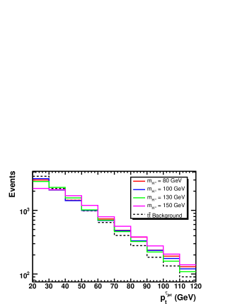
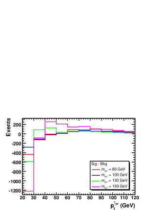
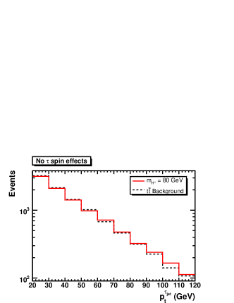
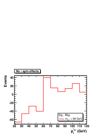
Figure 14.2.60: $p_{t}$ distributions of the $\tau~{}{\mathrm{jet}}$ for the $tbH^{\pm}$ signal and the $t\bar{t}$ background for $\sqrt{s}=1.96$ TeV (left) and the respective differences between signal and background (right). The lower plots show distributions without spin effects in the $\tau$ decays.

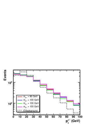
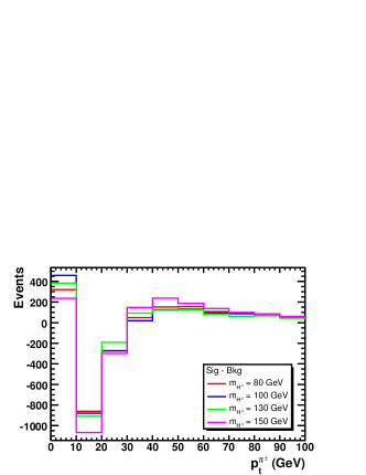
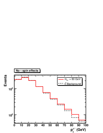
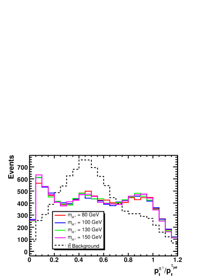
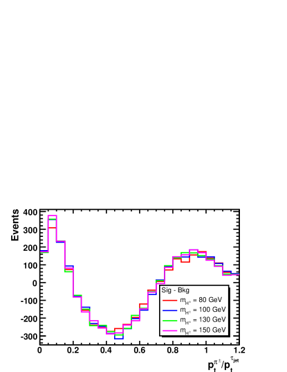
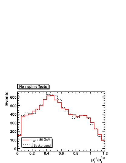
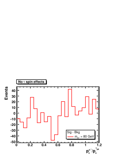
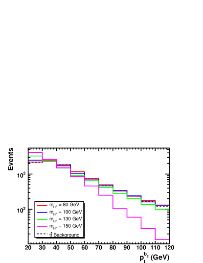
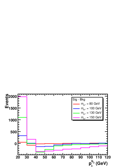
Figure 14.2.61: $p_{t}$ distributions of the leading $\pi^{\pm}$ from the $\tau$ decay for the $tbH^{\pm}$ signal and the $t\bar{t}$ background for $\sqrt{s}=1.96$ TeV (left) and the respective differences between signal and background (right). The lower plots show distributions without spin effects in the $\tau$ decays.

Figure 14.2.62: Distributions of the ratio $p_{t}^{\pi^{\pm}}/p_{t}^{\tau_{\mathrm{jet}}}$ for the $tbH^{\pm}$ signal and the $t\bar{t}$ background for $\sqrt{s}=1.96$ TeV (left) and the respective differences between signal and background (right). The lower plots show distributions without spin effects in the $\tau$ decays.

Figure 14.2.63: $p_{t}$ distributions of the second (least energetic) $b$ quark jet for the $tbH^{\pm}$ signal and the $t\bar{t}$ background for $\sqrt{s}=1.96$ TeV (left) and the respective differences between signal and background (right).

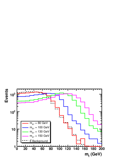
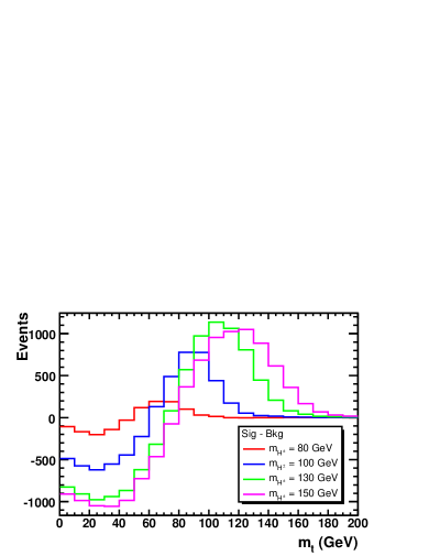
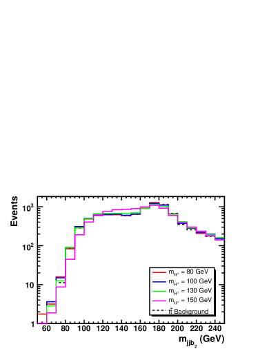
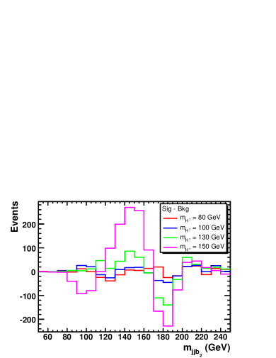
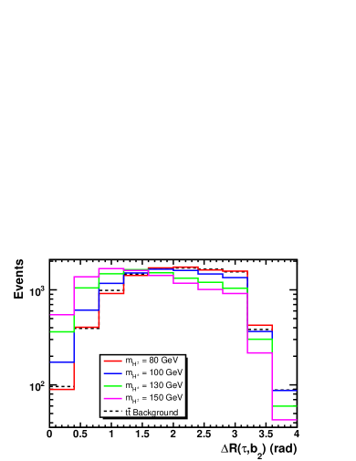
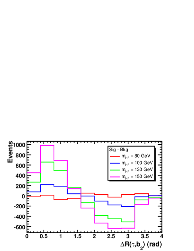
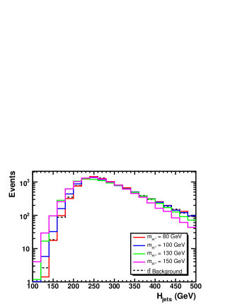
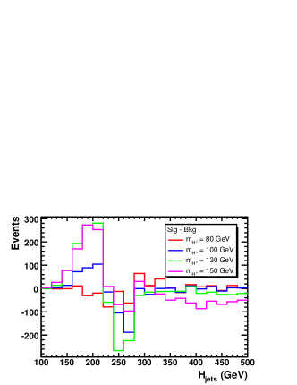
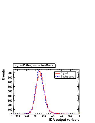
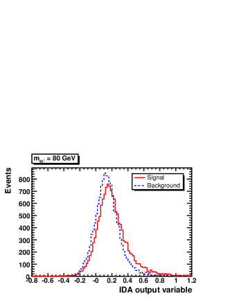
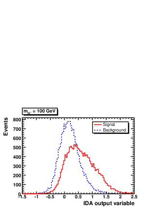
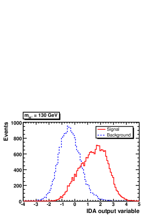
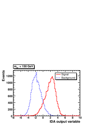
Figure 14.2.64: Transverse mass $m_{t}=\sqrt{2p_{t}^{\tau_{\mathrm{jet}}}p_{t}^{\rm miss}[1-\cos(\Delta\phi)]}$ distributions of the $\tau_{\rm jet}+p_{t}^{\rm miss}$ system ($\Delta\phi$ is the azimuthal angle between $p_{t}^{\tau_{\mathrm{jet}}}$ and $p_{t}^{\rm miss}$) for the $tbH^{\pm}$ signal and the $t\bar{t}$ background for $\sqrt{s}=1.96$ TeV (left) and the respective differences between signal and background (right).

Figure 14.2.65: Invariant mass distributions of the two light quark jets and the second (least energetic) $b$ quark jet for the $tbH^{\pm}$ signal and the $t\bar{t}$ background for $\sqrt{s}=1.96$ TeV (left) and the respective differences between signal and background (right).

Figure 14.2.66: Spatial distance $\Delta R(\tau,b_{2})=\sqrt{(\Delta\phi)^{2}+(\Delta\eta)^{2}}$ distributions (where $\Delta\phi$ is the azimuthal angle in rad between the $\tau$ and $b$ jet) for the $tbH^{\pm}$ signal and the $t\bar{t}$ background for $\sqrt{s}=1.96$ TeV (left) and the respective differences between signal and background (right).

Figure 14.2.67: Distributions of the total transverse momentum of all quark jets, $H_{\rm jets}=p_{t}^{j_{1}}+p_{t}^{j_{2}}+p_{t}^{b_{1}}+p_{t}^{b_{2}}$, for the $tbH^{\pm}$ signal and the $t\bar{t}$ background for $\sqrt{s}=1.96$ TeV (left) and the respective differences between signal and background (right).

Figure 14.2.68: Distributions of the IDA output variable in the first IDA step for the $tbH^{\pm}$ signal (solid, red) and the $t\bar{t}$ background (dashed, blue) for $\sqrt{s}=1.96$ TeV.

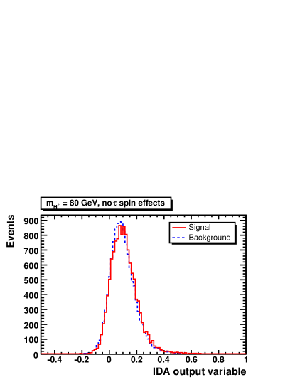
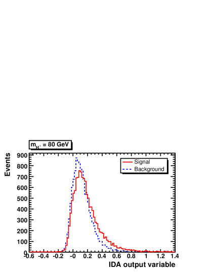
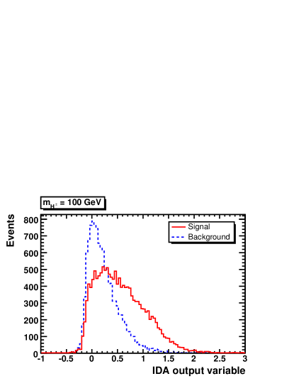
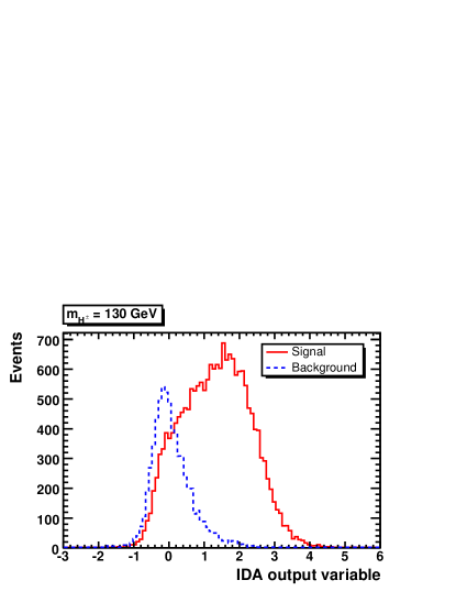
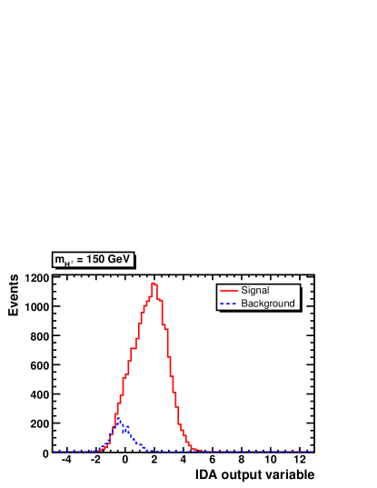
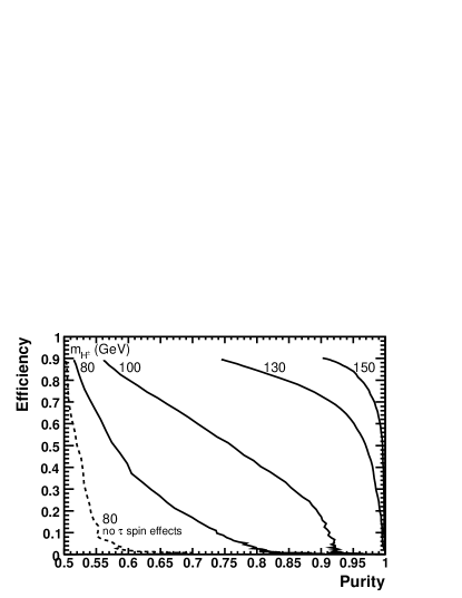
Figure 14.2.69: Upper row, middle row and lower left figure: distributions of the IDA output variable in the second IDA step for 90% efficiency in the first IDA step (corresponding to a cut at 0 in Fig. 14.2.68) for the $tbH^{\pm}$ signal (solid, red) and the $t\bar{t}$ background (dashed, blue). Lower right figure: efficiency as a function of the purity when not taking the spin effects in the $\tau$ decay into account for $m_{H^{\pm}}=80$ GeV (dashed) and with spin effects in the $\tau$ decay for $m_{H^{\pm}}=80,100,130,150$ GeV (solid, from left to right). Results are for the Tevatron.

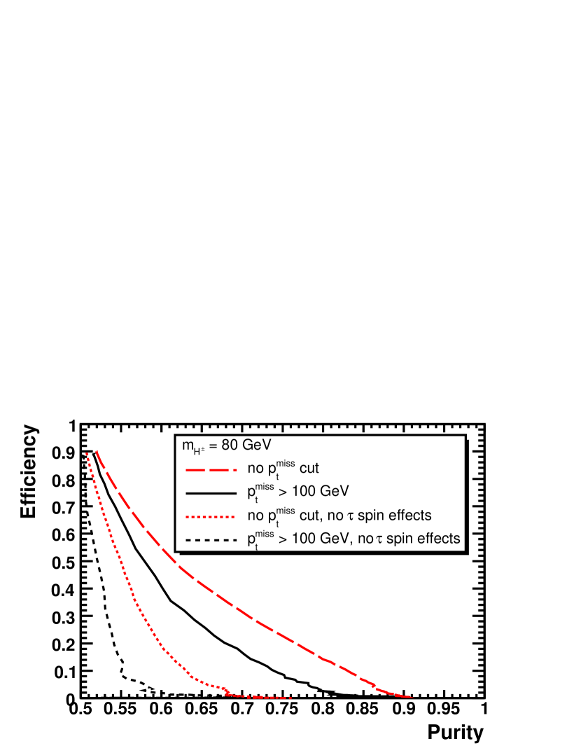
Figure 14.2.70: Efficiency as a function of purity for $m_{H^{\pm}}=80$ GeV and $\sqrt{s}=1.96$ TeV. The black lines are the results after applying the hard cut $p_{t}^{\rm miss}>100$ GeV when not taking the spin effects in the $\tau$ decay into account (dashed) and with spin effects in the $\tau$ decay (solid), as also shown in Fig.14.2.69. The red lines are the results without applying the hard cut on $p_{t}^{\rm miss}$ when not taking the spin effects in the $\tau$ decay into account (dotted) and with spin effects in the $\tau$ decay (long dashed).

14.3 LHC energy

The simulation procedure and the emulation of the detector response are the same as those outlined in Sect. 2.1 for the Tevatron, as well as, for the preselection and IDA method, as described in Sects. 2.3 and 2.4, respectively. Hence, only the expected LHC rates are discussed, followed by the description of changes in the distributions of the variables and the final IDA results.

Unlike the case of the Tevatron, where only charged Higgs masses smaller than the top quark mass can be explored, and 2HDM/MSSM signatures practically rely on $\tau\nu_{\tau}$ pairs only, at the LHC the phenomenology is more varied. Here, the search strategies depend strongly on the charged Higgs boson mass. If $m_{H^{\pm}}<m_{t}-m_{b}$ (later referred to as a light Higgs boson), the charged Higgs boson can be produced in top (anti-)quark decay. The main source of top (anti-)quarks at the LHC is again $t\bar{t}$ pair production ($\sigma_{t\bar{t}}=850$ pb at NLO) [340]. For the whole ($\tan\beta,m_{H^{\pm}}$) parameter space there is a competition between the $bW^{\pm}$ and $bH^{\pm}$ channels in top decay keeping the sum $\mathrm{BR}(t\to bW^{+})+\mathrm{BR}(t\to bH^{+})$ at almost unity. The top quark decay to $bW^{\pm}$ is however the dominant mode for most of the parameter space. Thus, the best way to search for a (light) charged Higgs boson is by requiring that the top quark produced in the $tbH^{\pm}$ process decays to a $W^{\pm}$. While in the case of $H^{\pm}$ decays $\tau$’s will be tagged via their hadronic decay producing low-multiplicity narrow jets in the detector, there are two different $W^{\pm}$ decays that can be explored. The leptonic signature $b\bar{b}H^{\pm}W^{\mp}\to b\bar{b}\tau\nu l\nu$ provides a clean selection of the signal via the identification of the lepton $l=e,\mu$. In this case the charged Higgs transverse mass cannot be reconstructed because of the presence of two neutrinos with different origin. In this channel charged Higgs discovery will be determined by the observation of an excess of such events over SM expectations through a simple counting experiment. In the case of hadronic decays $b\bar{b}H^{\pm}W^{\mp}\to b\bar{b}\tau\nu jj$ the transverse mass can instead be reconstructed since all neutrinos are arising from the charged Higgs boson decay. This allows for an efficient separation of the signal and the main $t\bar{t}\to b\bar{b}W^{\pm}W^{\mp}\to b\bar{b}\tau\nu jj$ background (assuming $m_{H^{\pm}}\lower 3.01385pt\hbox{$\;\stackrel{{\scriptstyle\textstyle>}}{{\sim}}\;$}m_{W^{\pm}}$). The absence of a lepton ($e$ or $\mu$) provides a less clean environment but the use of the transverse mass makes it possible to reach the same mass discovery region as in the previous case and also to extract the charged Higgs boson mass. Both these channels show that after an integrated luminosity of 30 fb^-1 the discovery could be possible up to a mass of 150 GeV for all tan$\beta$ values in both ATLAS and CMS [314, 341, 342].

If the charged Higgs is heavier than the top quark, the dominant decay channels are $H^{\pm}\to\tau\nu$ and $H^{\pm}\to tb$ depending on $\tan\beta$. They have both been studied by ATLAS and CMS [343, 344, 345, 346]. The charged Higgs bosons are produced in the $pp\to tbH^{\pm}$ channel. For the $H^{\pm}\to tb$ decay, a charged Higgs boson can be discovered up to high masses ($m_{H^{\pm}}\sim 400$ GeV) in the case of very large $\tan\beta$ values and this reach cannot be much improved because of the large multi-jet environment. For the $H^{\pm}\to\tau\nu$ decay mode this reach is larger due to a cleaner signal despite a lower BR. In this case the 5$\sigma$ reach ranges from $\tan\beta=20$ for $m_{H^{\pm}}=200$ GeV to $\tan\beta=30$ for $m_{H^{\pm}}=400$ GeV.

For the LHC, signal and background events have been simulated in the same way as for the Tevatron as described before, however, without implying any rescaling factor to match a measured $t\bar{t}$ cross section. Table 14.3.21 lists the resulting cross sections before ($\sigma^{\rm th}$) and after ($\sigma$) applying the basic cuts $p_{t}^{\rm jets}>20$ GeV and the hard cut $p_{t}^{\rm miss}>100$ GeV. The LHC rates allow for the discovery to be less challenging than at the Tevatron in the region $m_{H^{\pm}}\sim m_{W^{\pm}}$, yet the separation of signal events from background remains crucial for the measurement of the charged Higgs mass.

	$q\bar{q},gg\to t\bar{t}$	$q\bar{q},gg\to tbH^{\pm}$
$m_{H^{\pm}}$ (GeV)	80	80	100	130	150
$\sigma^{\rm th}$ (pb)	45.5	72.6	52.0	24.5	9.8
$\sigma$ (pb) for $p_{t}^{\mathrm{jets}}>20$ GeV	17.3	33.9	25.7	12.2	3.8
$\sigma$ (pb) for $(p_{t}^{\mathrm{jets}},p_{t}^{\rm miss})>(20,100)$ GeV	4.6	6.0	4.8	2.9	1.2

Table 14.3.21: LHC cross sections of background $q\bar{q},gg\to t\bar{t}$ and signal $q\bar{q},gg\to tbH^{\pm}$ for $\tan\beta=30$ and $m_{H^{\pm}}=80,100,130$ and $150$ GeV into the final state $2b+2j+\tau_{\mathrm{jet}}+p_{t}^{\rm miss}$ before ($\sigma^{\rm th}$) and after ($\sigma$) the basic cuts ($p_{t}>20$ GeV for all jets) and the hard cut ($p_{t}^{\rm miss}>100$ GeV).

The kinematic distributions are shown in Figs. 14.3.71 to 14.3.78 for $\sqrt{s}=14$ TeV. The choice of variables is identical to the one for the Tevatron and allows for a one-to-one comparison, the differences being due to a change in CM energy (and, to a somewhat lesser extent, due to the leading partonic mode of the production process). The main differences with respect to Figs. 14.2.60–14.2.67 are that the various transverse momenta and invariant masses have longer high energy tails. In particular, it should be noted that the effect of the spin differences between $W^{\pm}$ and $H^{\pm}$ events can be explored very effectively also at LHC energies, e.g. the ratio $p_{t}^{\pi^{\pm}}/p_{t}^{\tau_{\mathrm{jet}}}$ is shown in Fig. 14.3.73 which is very sensitive to the spin effects. These observations lead to the conclusion that the same method using spin differences can be used to separate signal from background at both the Tevatron and the LHC.

The distributions of the IDA output variables for the study at $\sqrt{s}=14$ TeV for two steps with 90% efficiency in the first step are shown in Figs. 14.3.79 and 14.3.80. These distributions are qualitatively similar to those for the Tevatron (Figs. 14.2.68 and 14.2.69) and the final achievable purity for a given efficiency is shown in Fig. 14.3.80. As for the Tevatron energy a good separation of signal and background events can be achieved with the spin sensitive variables and the IDA method even in case $m_{H^{\pm}}\sim m_{W^{\pm}}$. For heavier $H^{\pm}$ masses the separation of signal and background events increases due to the kinematic differences of the event topology.

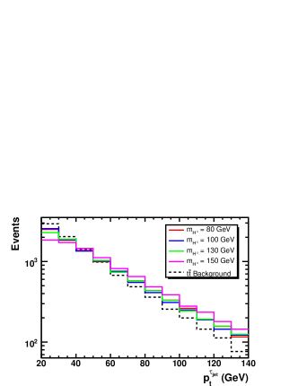
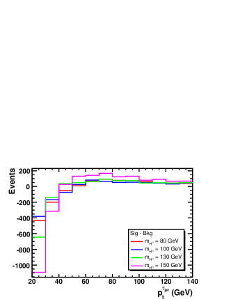
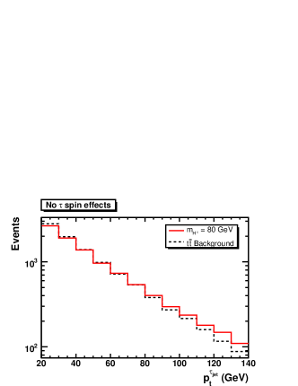
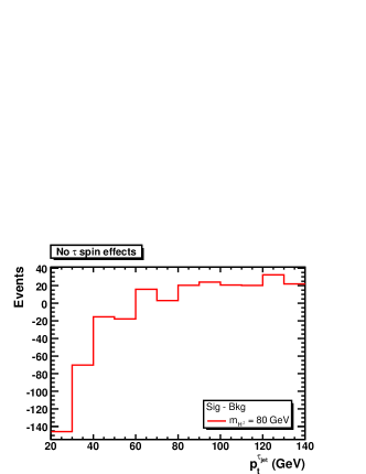
Figure 14.3.71: $p_{t}$ distributions of the $\tau~{}{\mathrm{jet}}$ for the $tbH^{\pm}$ signal and the $t\bar{t}$ background for $\sqrt{s}=14$ TeV (left) and the respective differences between signal and background (right). The lower plots show distributions without spin effects in the $\tau$ decays.

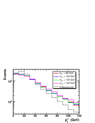
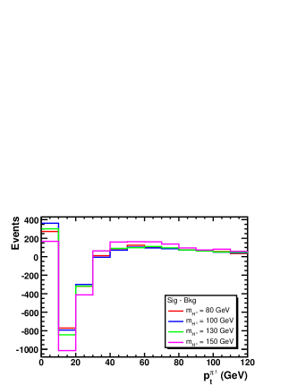
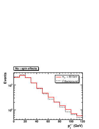
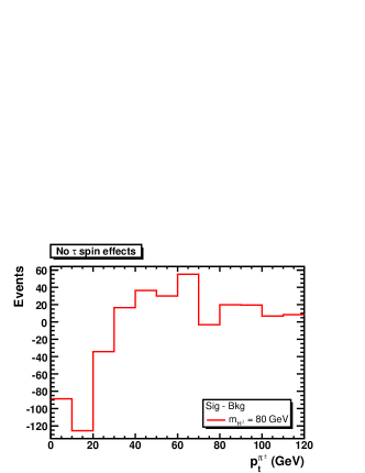
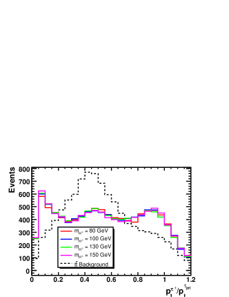
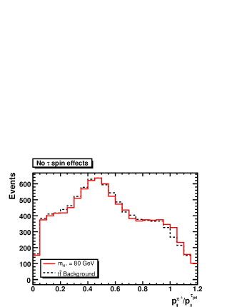
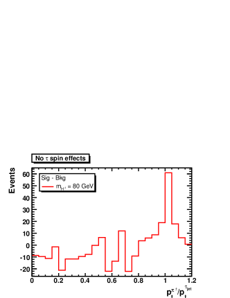
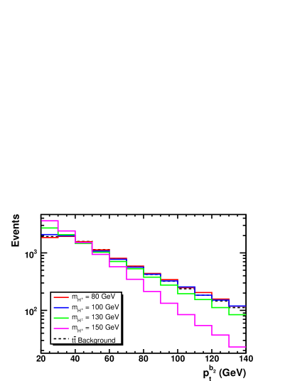
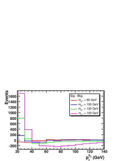
Figure 14.3.72: $p_{t}$ distributions of the leading $\pi^{\pm}$ from the $\tau$ decay for the $tbH^{\pm}$ signal and the $t\bar{t}$ background for $\sqrt{s}=14$ TeV (left) and the respective differences between signal and background (right). The lower plots show distributions without spin effects in the $\tau$ decays.

Figure 14.3.73: Distributions of the ratio $p_{t}^{\pi^{\pm}}/p_{t}^{\tau_{\mathrm{jet}}}$ for the $tbH^{\pm}$ signal and the $t\bar{t}$ background for $\sqrt{s}=14$ TeV (left) and the respective differences between signal and background (right). The lower plots show distributions without spin effects in the $\tau$ decays.

Figure 14.3.74: $p_{t}$ distributions of the second (least energetic) $b$ quark jet for the $tbH^{\pm}$ signal and the $t\bar{t}$ background for $\sqrt{s}=14$ TeV (left) and the respective differences between signal and background (right).

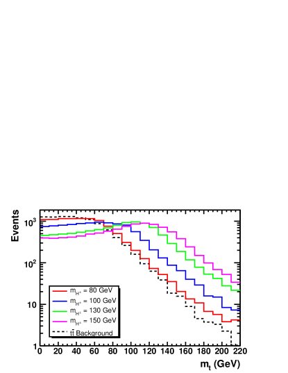
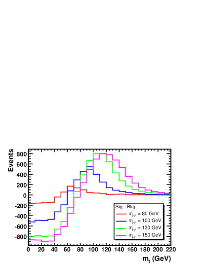
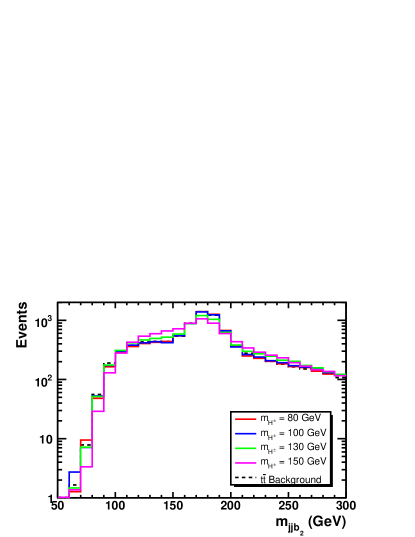
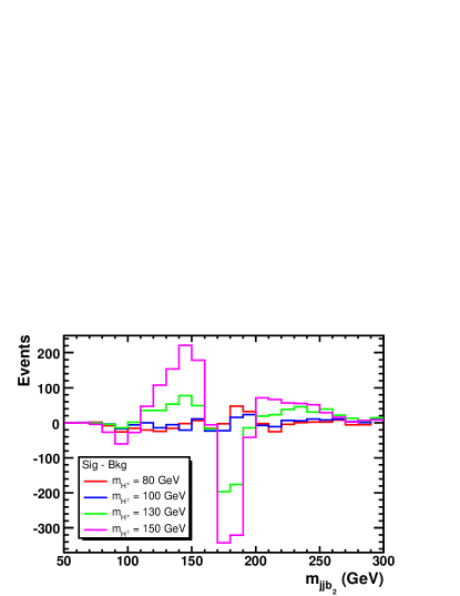
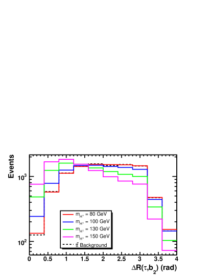
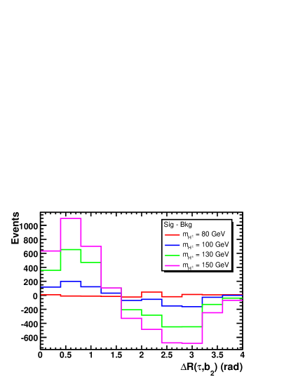
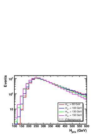
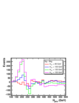
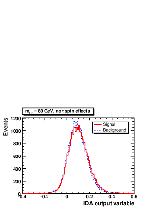
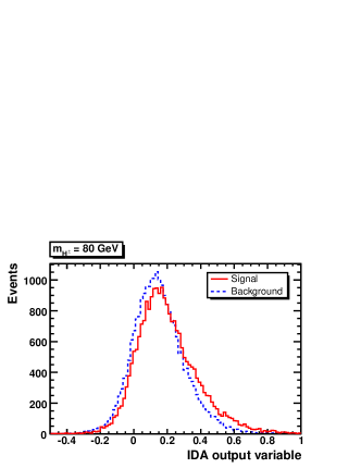
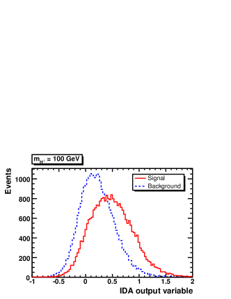
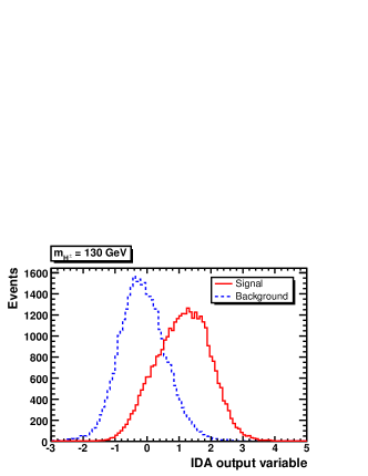
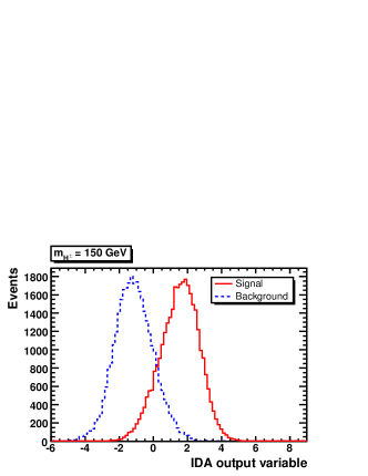
Figure 14.3.75: Transverse mass $m_{t}=\sqrt{2p_{t}^{\tau_{\mathrm{jet}}}p_{t}^{\rm miss}[1-\cos(\Delta\phi)]}$ distributions of the $\tau_{\rm jet}+p_{t}^{\rm miss}$ system ($\Delta\phi$ is the azimuthal angle between $p_{t}^{\tau_{\mathrm{jet}}}$ and $p_{t}^{\rm miss}$) for the $tbH^{\pm}$ signal and the $t\bar{t}$ background for $\sqrt{s}=14$ TeV (left) and the respective differences between signal and background (right).

Figure 14.3.76: Invariant mass distributions of the two light quark jets and the second (least energetic) $b$ quark jet for the $tbH^{\pm}$ signal and the $t\bar{t}$ background for $\sqrt{s}=14$ TeV (left) and the respective differences between signal and background (right).

Figure 14.3.77: Spatial distance $\Delta R(\tau,b_{2})=\sqrt{(\Delta\phi)^{2}+(\Delta\eta)^{2}}$ distributions (where $\Delta\phi$ is the azimuthal angle in rad between the $\tau$ and $b$ jet) for the $tbH^{\pm}$ signal and the $t\bar{t}$ background for $\sqrt{s}=14$ TeV (left) and the respective differences between signal and background (right).

Figure 14.3.78: Distributions of the total transverse momentum of all quark jets, $H_{\rm jets}=p_{t}^{j_{1}}+p_{t}^{j_{2}}+p_{t}^{b_{1}}+p_{t}^{b_{2}}$, for the $tbH^{\pm}$ signal and the $t\bar{t}$ background for $\sqrt{s}=14$ TeV (left) and the respective differences between signal and background (right).

Figure 14.3.79: Distributions of the IDA output variable in the first IDA step for the $tbH^{\pm}$ signal (solid, red) and the $t\bar{t}$ background (dashed, blue) for $\sqrt{s}=14$ TeV.

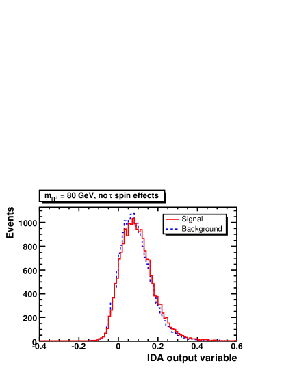
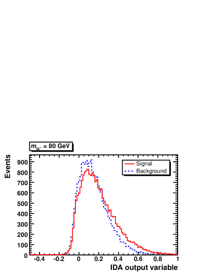
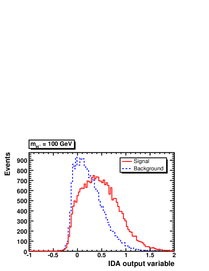
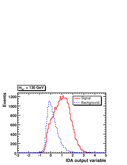
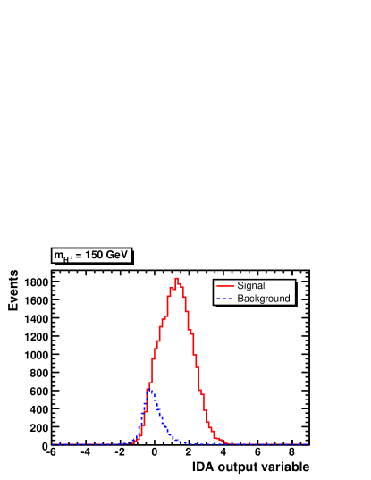
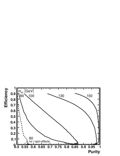
Figure 14.3.80: Upper row, middle row and lower left figure: distributions of the IDA output variable in the second IDA step for 90% efficiency in the first IDA step (corresponding to a cut at 0 in Fig. 14.3.79) for the $tbH^{\pm}$ signal (solid, red) and the $t\bar{t}$ background (dashed, blue). Lower right figure: efficiency as a function of the purity when not taking the spin effects in the $\tau$ decay into account for $m_{H^{\pm}}=80$ GeV (dashed) and with spin effects in the $\tau$ decay for $m_{H^{\pm}}=80,100,130,150$ GeV (solid, from left to right). Results are for the LHC.

14.4 Conclusions

The discovery of charged Higgs bosons would be a clear sign of physics beyond the SM. In this case study we have investigated charged Higgs boson topologies produced at the current Tevatron and LHC energies and compared them against the irreducible SM background due to top-antitop production and decay. While sizable differences between signal and background are expected whenever $m_{H^{\pm}}\neq m_{W^{\pm}}$, near the current mass limit of about $m_{H^{\pm}}\approx 80$ GeV the kinematic spectra are very similar between SM decays and those involving charged Higgs bosons. In this case, spin information will significantly distinguish between signal and irreducible SM background. In fact, we have considered hadronic $\tau\nu_{\tau}$ decays of charged Higgs bosons, wherein the $\tau$ polarization induced by a decaying (pseudo)scalar object is significantly different from those emerging in the vector ($W^{\pm}$) decays onsetting in the top-antitop case. For a realistic analysis which is not specific for a particular detector, a dedicated Monte Carlo event generation and a simplified multipurpose detector response approximation have been applied. The identification of a hadronic tau-lepton will be an experimental challenge in an environment with typically four jets being present. We have demonstrated how an IDA method can be an applied to separate signal and background when the differences between the signal and background distributions are small. Our results show that the IDA method will be equally effective at both the Tevatron and LHC. While only the dominant irreducible $t\bar{t}$ background has been dealt with in detail, we have also specifically addressed the QCD background. A suitably hard missing transverse momentum cut has been applied to reject such jet activity and we have demonstrated that although the discriminative power is reduced by such a cut, the reduction is small compared to the gain from including the $\tau$ polarization effects. Using the differences in $\tau$ polarization between the signal and the dominant SM irreducible $t\bar{t}$ background is crucial for disentangling the former from the latter.

15 Energy scale for b jets in DØ

Contributed by: J. Cammin

This section describes the determination of the energy response of b jets in the DØ calorimeter. Since this measurement is work in progress, and no final results are available yet, we discuss only the concept of the measurement.

15.1 Introduction

In DØ, jet energies measured in the calorimeter [347], are corrected for offset, response, and showering [348]. The response is the largest single correction factor and is measured from the energy balance in $\gamma+$jets events using the “Missing $E_{T}$ Projection Fraction Method” (MPF) [348]. The response is measured in bins of an energy estimator, $E^{\prime}=E_{T_{\gamma}}\cosh(\eta_{\mathrm{jet}})$, which later is mapped to the raw measured jet energy, $E_{\mathrm{jet}}^{\mathrm{meas}}$ in order to get an energy-dependent measurement of the jet response.

The above mentioned corrections are derived for light jets and do not take into account peculiarities of heavy flavor jets, such as different fragmentation and hadronization and the presence of semileptonic decays. The latter leads to an energy response considerably smaller than that of light jets because of the neutrino involved in the decay. It is therefore crucial to derive special energy corrections for b jets, so that particle masses measured in decays containing b quarks, such as $\mathrm{Z\to b\bar{b}}$, $\mathrm{t\to bW}$, or $\mathrm{H\to b\bar{b}}$, are reconstructed at the correct energy scale.

In DØ special b jet corrections exist only for semi-muonic decays, which are applied if the jet contains a “soft” muon. The following section describes the response measurement to compensate for the remaining effects (mainly due to semi-electronic decays, for which no dedicated corrections exist).

15.2 The concept of the measurement

The response for b jets that do not have a soft muon tag is measured in b-tagged $\gamma+$jets events using the same method (MPF) as for the light jet response described above. However, b-tagged jets are a mixture of true b and c jets and mistagged light jets which have different energy responses. The situation is sketched in Figure 15.2.82, where the measured mean value of the response distribution in a particular energy bin is the weighted sum of the mean values of response distributions for light, b, and c jets. The response of b jets thus needs to be disentangled from the response measured in a tagged $\gamma+$jets sample. Since there are three unknows, the mean values $\mathrm{R_{j}}$, $\mathrm{R_{b}}$, and $\mathrm{R_{c}}$ of the responses, this can be accomplished by algebraically solving a system of three equations, where each equation corresponds to a measurement of the response in a sample with different flavor composition of the jets. In DØ, the first measurement is performed on an untagged sample. With good approximation, the measured response is that of light jets, $\mathrm{R_{j}}$, Equation (15.2.97). The second measurement is obtained from a b-tagged $\gamma+$jets sample using the “counting signed impact parameter” (Csip) algorithm [349], Equation (15.2.98). The third equation is taken from a sample with a tighter b-tagging criterion: The jets must be tagged with the Csip algorithm and have a “track mass” $m_{\mathrm{trk}}$ above 1.93 GeV, Equation (15.2.99). $m_{\mathrm{trk}}$ is the invariant mass of the tracks that tag the jet, i.e., tracks with impact parameter significance greater than two.

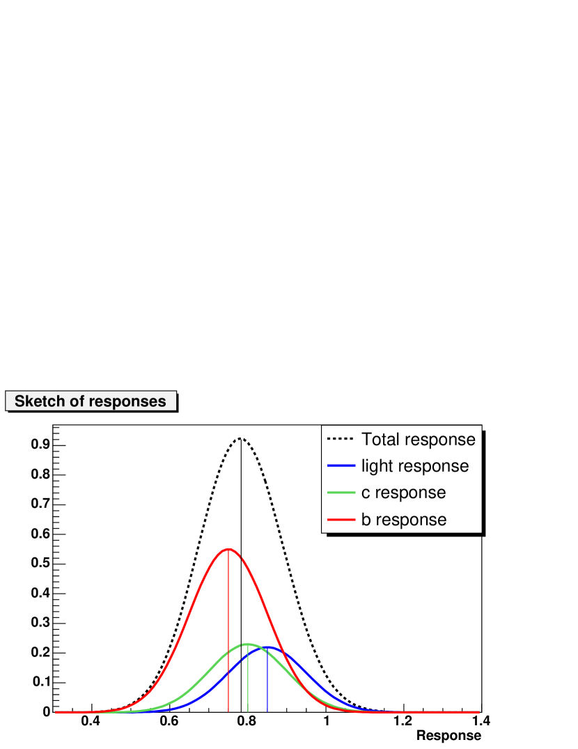
Figure 15.2.81: Sketch of response distribution in a particular energy bin.

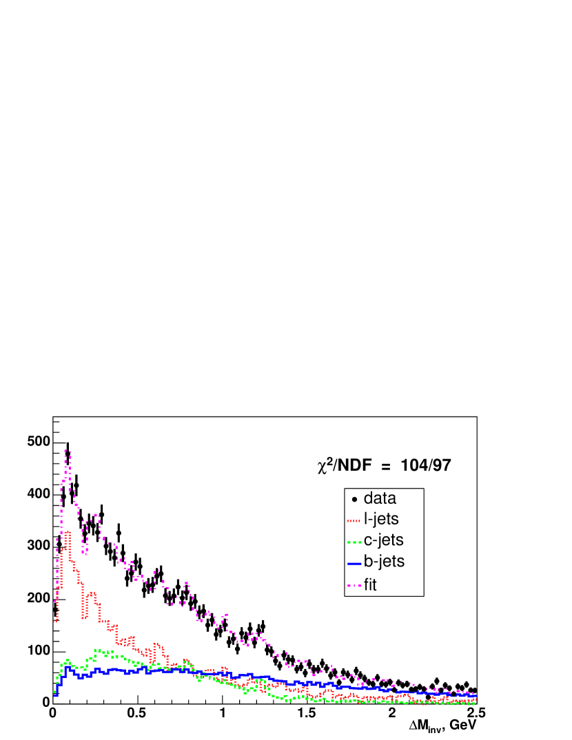
Figure 15.2.82: “Invariant track mass” minus an offset of $m_{\pi}+m_{K}$.

$$\mathrm{untagged:}\qquad R_{ut} \approx R_{l}$$ (15.2.97)

$$\mathrm{tagged:}\qquad R_{t} = f_{l}R_{l}+f_{b}R_{b}+f_{c}R_{c}$$ (15.2.98)

$$\mathrm{tagged:}\qquad R_{mt} = f^{\prime}_{l}R_{l}+f^{\prime}_{b}R_{b}+f^{\prime}_{c}R_{c}$$ (15.2.99)

The distribution of the invariant mass $m_{\mathrm{trk}}$ is depicted in Figure 15.2.82 for light, b, and c jets. The energy response of b jets is then obtained by solving the system of Equations (15.2.97)– (15.2.99) and measuring $R_{ut}$, $R_{t}$, and $R_{mt}$ in various energy bins:

$$R_{b}=\frac{1}{f_{b}-\frac{f_{c}}{f_{c}^{\prime}}f_{b}^{\prime}}\left[R_{t}-R_{ut}\left(f_{l}-\frac{f_{c}}{f_{c}^{\prime}}f_{l}^{\prime}\right)-R_{mt}\frac{f_{c}}{f_{c}^{\prime}}\right].$$ (15.2.100)

The flavor fractions $f^{(^{\prime})}_{l},f^{(^{\prime})}_{b},f^{(^{\prime})}_{c}$ can be obtained from fits of the mass templates to the data distribution as shown in Figure 15.2.82, or from a similar distribution that discriminates between the jet flavors. The flavor composition is also a function of the energy and must be measured separately in each energy bin.

The advantage of this method is that the energy response of b jets is measured directly in data and relies only very little on Monte Carlo simulations (template distributions for the fit to the flavor fractions). However, an inclusive $\gamma+$jets sample contains only a few percent of $\gamma+$b events, hence a large data sample is needed in order to keep the statistical uncertainties at a reasonable level.

Since jets in DØ are already corrected for the light jet energy scale, the resulting b response will be provided as a residual scale factor $\mathrm{R_{j}}$/$\mathrm{R_{b}}$. This scale factor derived from tagged $\gamma+$jets data can also be compared to Monte Carlo simulations of $\gamma+$jets and $\gamma+$b events, a preliminary result of which is shown in Figure 15.2.83. The study suggests that b jets need additional energy corrections of as much as 10% at energies around 20 GeV and about 5% at energies of 150 GeV.

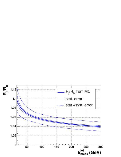
Figure 15.2.83: Response of b jets relative to the light jet response as a function of the raw jet energy.

16 Insights into $H\rightarrow\gamma\gamma$ from CDF Searches

Contributed by: S.-W. Lee

We describe how all of the diphoton measurements at CDF provide important insights into the Higgs search at the LHC, $H\rightarrow\gamma\gamma$. A brief review of diphoton physics at CDF is also given here.

16.1 Introduction

The study of photon production at a hadron collider is important for many reasons. As the photon energy is well-measured, compared to jets, it can be a good tool to further our understanding of Quantum Chromodynamics (QCD). One of the important reason to study photons at a hadron collider, as well as all QCD measurements, is that they are the backgrounds to new physics. The most famous of these is the Higgs search at the LHC, where diphoton backgrounds are the most serious experimental difficulty. In the next section we will illustrate how all of the diphoton measurements at CDF provide important insights into backgrounds for new physics, specifically the diphoton backgrounds to the Higgs search at the LHC, $H\rightarrow\gamma\gamma$.

In addition, there are a large number of important and well-motivated theoretical models which make a strong case for looking for new physics in events with two photons in the final state. These theories include Supersymmetry (SUSY), Extra Dimensions (ED), Grand Unified Theories, Composite models of quarks and leptons, and Technicolor models. Therefore it is important to understand diphoton production at Tevatron experiments in order to reliably search for the Standard Model Higgs and new physics at LHC.

The aim of this talk is to present the recent measurement of diphoton production at Tevatron experiment, CDF, to lead us to a deeper understanding of new physics signatures at LHC experiments.

16.2 Diphoton physics at CDF

A brief review of physics with diphoton final states using the CDF detector at the Tevatron is given here. These include searches for supersymmetry, extra dimensions and bosophilic Higgs, as well as QCD diphoton cross section measurement. Recent results from CDF Run II experiment are presented, but some result from Run I is also reviewed.

Diphoton final states are a signature of many interesting processes. For example, at the LHC, one of the main discovery channels for the Higgs boson search is the $\gamma\gamma$ final state. An excess of $\gamma\gamma$ production at high invariant mass could be a signature of large extra dimensions, and in many theories involved physics beyond the standard model, cascade decays of heavy new particles generate a $\gamma\gamma$ signature in the final state. However, the QCD production rate is large compared to most new physics, so an understanding of the QCD production mechanism is a prerequisite to searching reliably for new physics in this channel.

CDF has good analysis tool to identify the photon signal from the mixture of photons and a neutral meson background. For the CDF measurement the fraction of photon candidate events that have an observed conversion in the materials just in front of the calorimeter is used, along with the transverse shower shape measured in a proportional chamber at shower maximum in the calorimeter itself. In the end one of the two methods is used to evaluate point-by-point the fraction of photons in the data sample. [350].

Diphoton Cross Section

Recently CDF has performed pure QCD test with prompt diphotons using a data sample of 207 $pb^{-1}$ in Run II [351]. The analysis required two photon candidates with $E_{T}>$ 14 GeV (13 GeV) for the leading (softer) photon candidate in the event. The background from non-prompt photon sources is determined using a statistical method based on differences in the electromagnetic showers.

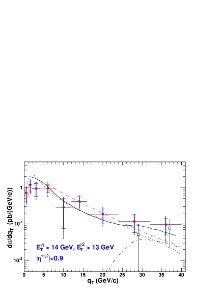
Figure 16.2.84: The $\gamma\gamma$ $q_{T}$ distribution, along with predictions from DIPHOX (solid), RESBOS (dashed), and PYTHIA (dotted). The PYTHIA predictions have been scaled by a factor of 2. Also shown, at larger $q_{T}$, are the DIPHOX prediction (dot-dashed) and the CDF data (open squares) for the configuration where the two photons are required to have $\Delta\phi<\pi/2$.

CDF has measured the cross section for prompt diphoton production as a function of three kinematic variables - diphoton mass, the transverse momentum of the diphoton system ($q_{T}$), and the azimuthal angle between the two photons, $\Delta\phi$. Comparisons have been made with predictions from DIPHOX, RESBOS and PYTHIA. The data are in good agreement with the predictions for the mass distribution. At low to moderate $q_{T}$ and $\Delta\phi$ greater than $\pi/2$, where the effect of soft gluon emissions are important, the data agree better with RESBOS than DIPHOX. By contrast, in the regions where the 2$\rightarrow$3 fragmentation contribution becomes important, large $q_{T}$, $\Delta\phi$ less than $\pi/2$ and low diphoton mass, the data agree better with DIPHOX. The $q_{T}$ distribution is shown in Fig. 1.

This result would appear to indicate a need to have a full theoretical calculation of diphoton production; a resummed full NLO calculation will be necessary. Again, an understanding of the QCD diphoton production mechanism is a prerequisite to searching reliably for new physics in this channel.

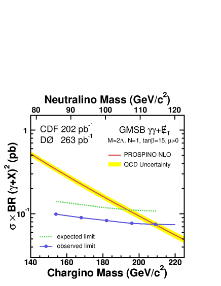
Figure 16.2.85: The NLO cross section and combined experimental limits as a function of chargino and neutralino mass in GMSB model.

Search for Supersymmetry

Among various SUSY models, two SUSY breaking mechanism are interesting, which predict photons in the final states. Supergravity models can produce events which decay down to the second lightest neutralino via a loop into the lightest neutralino ($\widetilde{\chi}_{1}^{0}$) and a photon, where $\widetilde{\chi}_{1}^{0}$ is the lightest supersymmetric particle (LSP). Gauge-Mediated SUSY breaking models (GMSB) with the $\widetilde{\chi}_{1}^{0}$ decaying into a photon and gravitino can produce a final state of two photons and large missing transverse energy ($\not\!\!E_{T}$). $\not\!\!E_{T}$ is often used as a pointer to possible SUSY signals because it indicates the escape of a non-interacting SUSY particle from the detector. The LSP signals are of particular interest as they provide a natural explanation for the dark matter.

CDF has searches 202 $pb^{-1}$ of inclusive diphoton events of Run II data for anomalous production of $\not\!\!E_{T}$ as evidence of new physics. Events are selected as having two photon candidates with $E_{T}>$ 13 GeV in the central. CDF observe no candidate events, with an expected standard model background of 0.27 $\pm$ 0.07 (stat) $\pm$ 0.10 (syst) events. Using these results, CDF has set limit on the lightest chargino M${}_{\mbox{$\widetilde{\chi}_{1}^{\pm}$}}>167$ GeV/$c^{2}$, and the lightest neutralino M${}_{\mbox{$\widetilde{\chi}_{1}^{0}$}}>93$ GeV/$c^{2}$ at 95% C.L. in a GMSB scenario with a light gravitino [352].

Fig. 2 shows the combined CDF and D0 result for the observed cross section as a function of $\widetilde{\chi}_{1}^{\pm}$ and $\widetilde{\chi}_{1}^{0}$ along with the theoretical LO and NLO production cross sections. The final mass limit for the lightest chargino is 209 GeV$/c^{2}$ which translates to a mass limit of 114 GeV$/c^{2}$ on the lightest neutralino and a limit of 84.6 TeV on $\Lambda$. This result significantly extends the individual experimental limits [353].

Search for Extra Dimensions

Recent theories postulate the existence of new space-time dimensions. Such extra dimensions might be found by looking for graviton exchange processes in the diphoton final state. For example in the Randall-Sandrum model with a warped extra dimension, diphoton resonances can be produced via the graviton.

CDF has searches for diphoton mass resonance with a data sample of 345 $pb^{-1}$. Two isolated photons , each with $E_{T}>$ 25 GeV, are required in the analysis. The main background comes from standard model diphoton production which accounts for 30% of the events, and from jets which fake photons. No deviation from standard model expectations is observed, and set upper limit on the cross section times branching ratio of the Randall-Sandrum graviton production and decay to diphotons. The lower mass bounds obtained for the first excited states of the Randall-Sandrum graviton are 690 and 220 GeV$/c^{2}$ for coupling, k/M_pl = 0.1 and 0.01, respectively. [354]

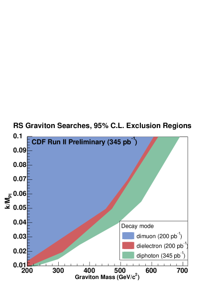
Figure 16.2.86: Combined 95% C.L. RS gaviton mass limit of the diphoton and dilepton searches

Fig. 3 shows the combined 95% C.L. RS graviton mass limit of the diphoton and dilepton searches in the graviton mass versus k/M_pl plane.

Search for Bosophilic Higgs

The signature of high mass photon pairs is attractive for searches for new physics as the photon is the lightest gauge boson, and hence might be more easily produced in decays of new physics. There are models in which a Higgs boson could decay into two photons with a branching ratio much larger than predicted in the standard model; bosophilic Higgs boson.

In Run I CDF has searched for departures from standard model expectations for inclusive high mass diphoton production in association with a W or Z boson [355]. This analysis is complimentary to the diphoton cross section analysis, in which very strict photon selection requirements are used to reduce the large jet fake backgrounds maximizing signal significance, but which become progressively less efficient with $E_{T}$ for high energy photons. It is also complimentary to the recent diphoton+X search analysis which was focused on non-resonant diphoton signatures such as GMSB SUSY.

Figure 16.2.87: Upper limit at 95% C.L. on the $\gamma\gamma+W/Z$  cross section as a function of $\gamma\gamma$ mass. The dashed curve shows the prediction for cross section times branching fraction for a bosophilic $H\to\gamma\gamma$ with branching fraction from reference [1] and the cross section for associa ted Higgs production is a standard model NLO calculation from reference [356].

CDF found no evidence for a resonant structure and set an upper limit on the cross section times branching ratio for $\mathrm{p}\bar{\mathrm{p}}\rightarrow H\rightarrow\gamma\gamma$ between 60 and 200 GeV/$c^{2}$ (see Fig. 4). A 95% C.L. lower limit on the mass of a bosophilic Higgs boson (one which couples only to $\gamma$, W and Z with standard model couplings) is set at 82 GeV/c².

16.3 Conclusion

In this article we summarize the current CDF experimental results of diphoton physics, test of standard model and searches for new physics in final states containing energetic photons, at Tevatron. we also describe how all of the diphoton measurements at CDF provide important insights into backgrounds for new physics, specifically the diphoton backgrounds to the Higgs search at the LHC. As we learned it is important to understand diphoton production in order to reliably search for the standard model Higgs and new physics. There may be an interesting connection between Tevatron and LHC.

References

- [1] A. Stange, W. J. Marciano and S. Willenbrock, Phys. Rev. D49, 1354 (1994), [hep-ph/9309294].
- [2] T. Han and R.-J. Zhang, Phys. Rev. Lett. 82, 25 (1999), [hep-ph/9807424].
- [3] TeV-2000 Study Group, D. Amidei et al., SLAC-REPRINT-1996-085.
- [4] Higgs Working Group, M. Carena et al., hep-ph/0010338.
- [5] ALEPH, DELPHI, L3 and OPAL Collaborations, and the LEP Electroweak Working Group, hep-ex/0511027.
- [6] LEP Higgs Working Group, Phys. Lett. B 565, 61 (2003), [hep-ex/0306033].
- [7] S. Heinemeyer, W. Hollik and G. Weiglein, 1998-1999, Phys. Rev. D 58 (1998) 091701, hep-ph/9803277; Phys. Lett. B 440 (1998) 296, hep-ph/9807423; Eur. Phys. J. C 9 (1999) 343, hep-ph/9812472.
- [8] G. Degrassi, S. Heinemeyer, W. Hollik, P. Slavich and G. Weiglein, Eur. Phys. J. C 28, 133 (2003), [hep-ph/0212020].
- [9] B. C. Allanach, A. Djouadi, J. L. Kneur, W. Porod and P. Slavich, JHEP 09, 044 (2004), [hep-ph/0406166].
- [10] M. G. Albrow and A. Rostovtsev, hep-ph/0009336.
- [11] V. A. Khoze, A. D. Martin and M. G. Ryskin, Eur. Phys. J. C23, 311 (2002), [hep-ph/0111078].
- [12] A. De Roeck, V. A. Khoze, A. D. Martin, R. Orava and M. G. Ryskin, Eur. Phys. J. C25, 391 (2002), [hep-ph/0207042].
- [13] B. E. Cox, AIP Conf. Proc. 753, 103 (2005), [hep-ph/0409144].
- [14] J. R. Forshaw, hep-ph/0508274.
- [15] S. Heinemeyer et al., Diffractive higgs production in the mssm, 2006, In preparation.
- [16] R. Harlander and W. Kilgore, Phys. Rev. Lett. 88, 201801 (2002), [hep-ph/0201206].
- [17] C. Anastasiou and K. Melnikov, Nucl. Phys. B 646, 220 (2002), [hep-ph/0207004].
- [18] V. Ravindran, J. Smith and W. van Neerven, Nucl. Phys. B 665, 325 (2003), [hep-ph/0302135].
- [19] D. Graudenz, M. Spira and P. Zerwas, Phys. Rev. Lett. 70, 1372 (1993).
- [20] M. Spira, A. Djouadi, D. Graudenz and P. M. Zerwas, Nucl. Phys. B453, 17 (1995), [hep-ph/9504378].
- [21] S. Moch and A. Vogt, Phys. Lett. B631, 48 (2005), [hep-ph/0508265].
- [22] E. Laenen and L. Magnea, Phys. Lett. B632, 270 (2006), [hep-ph/0508284].
- [23] S. Catani, D. de Florian, M. Grazzini and P. Nason, JHEP 07, 028 (2003), [hep-ph/0306211].
- [24] A. Martin, R. Roberts, W. Stirling and R. Thorne, Eur. Phys. J. C 28, 455 (2003), [hep-ph/0211080].
- [25] C. Anastasiou, K. Melnikov and F. Petriello, Phys. Rev. Lett. 93, 262002 (2004), [hep-ph/0409088].
- [26] U. Aglietti, R. Bonciani, G. Degrassi and A. Vicini, Phys. Lett. B 595, 432 (2004), [hep-ph/0404071].
- [27] G. Degrassi and F. Maltoni, Phys. Lett. B 600, 255 (2004), [hep-ph/0407249].
- [28] T. Han, G. Valencia and S. Willenbrock, Phys. Rev. Lett. 69, 3274 (1992), [hep-ph/9206246].
- [29] E. Berger and J. Campbell, Phys. Rev. D 70, 073011 (2004), [hep-ph/0403194].
- [30] T. Figy, C. Oleari and D. Zeppenfeld, Phys. Rev. D 68, 073005 (2003), [hep-ph/0306109].
- [31] J. M. Campbell and R. K. Ellis, Phys. Rev. D 60, 113006 (1999), [hep-ph/9905386].
- [32] J. Pumplin et al., JHEP 0207, 012 (2002), [hep-ph/0201195].
- [33] O. Brein, A. Djouadi and R. Harlander, Phys. Lett. B 579, 149 (2004), [hep-ph/0307206].
- [34] M. L. Ciccolini, S. Dittmaier and M. Krämer, Phys. Rev. D 68, 073003 (2003), [hep-ph/0306234].
- [35] Higgs Working Group Collaboration, K. A. Assamagan et al., hep-ph/0406152.
- [36] R. V. Harlander and W. B. Kilgore, Phys. Rev. D 68, 013001 (2003), [hep-ph/0304035].
- [37] S. Dittmaier, M. Krämer and M. Spira, Phys. Rev. D 70, 074010 (2004), [hep-ph/0309204].
- [38] S. Dawson, C. B. Jackson, L. Reina and D. Wackeroth, Phys. Rev. D 69, 074027 (2004), [hep-ph/0311067].
- [39] S. Dawson, C. B. Jackson, L. Reina and D. Wackeroth, Phys. Rev. Lett. 94, 031802 (2005), [hep-ph/0408077].
- [40] S. Dawson, C. B. Jackson, L. Reina and D. Wackeroth, Mod. Phys. Lett. A 21, 89 (2006), [hep-ph/0508293].
- [41] J. Campbell, R. K. Ellis, F. Maltoni and S. Willenbrock, Phys. Rev. D 67, 095002 (2003), [hep-ph/0204093].
- [42] W. Beenakker et al., Phys. Rev. Lett. 87, 201805 (2001), [hep-ph/0107081].
- [43] L. Reina and S. Dawson, Phys. Rev. Lett. 87, 201804 (2001), [hep-ph/0107101].
- [44] S. Dawson, L. H. Orr, L. Reina and D. Wackeroth, Phys. Rev. D 67, 071503 (2003), [hep-ph/0211438].
- [45] A. Ballestrero and E. Maina, Phys. Lett. B 299, 312 (1993).
- [46] F. Maltoni, K. Paul, T. Stelzer and S. Willenbrock, Phys. Rev. D 64, 094023 (2001), [hep-ph/0106293].
- [47] LEP Higgs working group, hep-ex/0107030, LHWG Note 2004-1, 2001, hep-ex/0107030, lephiggs.web.cern.ch/LEPHIGGS/papers.
- [48] V. Abazov et al., hep-ex/0504018, 2005, D0 Collaboration.
- [49] A. Abulencia et al., hep-ex/0508051, 2005, CDF Collaboration.
- [50] R. Eusebi, Search for charged Higgs in decay products from proton-antiproton collisions at , PhD thesis, University of Rochester, 2005, CDF Collaboration. hep-ex/0510065, CDF Note 7250.
- [51] M. Schumacher, Czech. J. Phys. 54, A103 (2004), [hep-ph/0410112].
- [52] M. Carena, S. Heinemeyer, C. Wagner and G. Weiglein, hep-ph/9912223, 1999.
- [53] M. Carena, S. Heinemeyer, C. Wagner and G. Weiglein, Eur. Phys. J. C 26, 601 (2003), [hep-ph/0202167].
- [54] M. Carena, S. Heinemeyer, C. Wagner and G. Weiglein, 2005, hep-ph/0511023, to appear in Eur. Phys. J. C.
- [55] S. Heinemeyer, W. Hollik and G. Weiglein, Comput. Phys. Commun. 124, 76 (2000), [hep-ph/9812320].
- [56] M. Carena et al., Nucl. Phys. B 580, 29 (2000), [hep-ph/0001002].
- [57] The Tevatron Electroweak Working Group, hep-ex/0507091, 2005.
- [58] S. Heinemeyer, W. Hollik and G. Weiglein, JHEP 0006, 009 (2000), [hep-ph/9909540].
- [59] A. Djouadi, Phys. Lett. B 435, 101 (1998), [hep-ph/9806315].
- [60] R. Harlander and M. Steinhauser, JHEP 0409, 066 (2004).
- [61] T. Hahn, S. Heinemeyer and G. Weiglein, Nucl. Phys. B652, 229 (2003), [hep-ph/0211204].
- [62] A. Belyaev, T. Han and R. Rosenfeld, JHEP 0307, 021 (2003), [hep-ph/0204210].
- [63] D. Cavalli et al., The Higgs working group: summary report, hep-ph/0203056, 2002.
- [64] S. Mrenna and J. D. Wells, Phys. Rev. D 63, 015006 (2001), [hep-ph/0001226].
- [65] R. Kinnunen, S. Lehti, A. Nikitenko and P. Salmi, J. Phys. G 31, 71 (2005), [hep-ph/0503067].
- [66] J. F. Gunion, H. E. Haber, G. L. Kane and S. Dawson, The Higgs Hunter’s Guide (Addison-Wesely, 1989), SCIPP-89/13.
- [67] J. F. Gunion, H. E. Haber, G. L. Kane and S. Dawson, Errata for the higgs hunter’s guide, hep-ph/9302272, 1993.
- [68] A. Djouadi, J. Kalinowski and M. Spira, Comput. Phys. Commun. 108, 56 (1998), [hep-ph/9704448].
- [69] L. Susskind, Phys. Rev. D20, 2619 (1979).
- [70] S. Weinberg, Phys. Rev. D13, 974 (1976).
- [71] S. Weinberg, Phys. Rev. D19, 1277 (1979).
- [72] E. Farhi and L. Susskind, Phys. Rept. 74, 277 (1981).
- [73] R. Casalbuoni et al., Nucl. Phys. B555, 3 (1999), [hep-ph/9809523].
- [74] K. D. Lane and M. V. Ramana, Phys. Rev. D44, 2678 (1991).
- [75] K. D. Lane, Phys. Rev. D60, 075007 (1999), [hep-ph/9903369].
- [76] A. Belyaev, A. Blum, R. S. Chivukula and E. H. Simmons, Phys. Rev. D72, 055022 (2005), [hep-ph/0506086].
- [77] M. Carena, S. Mrenna and C. E. M. Wagner, Phys. Rev. D60, 075010 (1999), [hep-ph/9808312].
- [78] M. Carena, S. Mrenna and C. E. M. Wagner, Phys. Rev. D62, 055008 (2000), [hep-ph/9907422].
- [79] S. Dawson, A. Djouadi and M. Spira, Phys. Rev. Lett. 77, 16 (1996), [hep-ph/9603423].
- [80] R. V. Harlander and M. Steinhauser, Phys. Lett. B 574, 258 (2003), [hep-ph/0307346].
- [81] R. Harlander and M. Steinhauser, Phys. Rev. D 68, 111701 (2003), [hep-ph/0308210].
- [82] R. V. Harlander and M. Steinhauser, JHEP 0409, 066 (2004), [hep-ph/0409010].
- [83] C. Balazs, H.-J. He and C. P. Yuan, Phys. Rev. D60, 114001 (1999), [hep-ph/9812263].
- [84] M. Spira, Nucl. Instrum. Meth. A389, 357 (1997), [hep-ph/9610350].
- [85] S. Dimopoulos, S. Raby and G. L. Kane, Nucl. Phys. B182, 77 (1981).
- [86] J. R. Ellis, M. K. Gaillard, D. V. Nanopoulos and P. Sikivie, Nucl. Phys. B182, 529 (1981).
- [87] B. Holdom, Phys. Rev. D24, 157 (1981).
- [88] DØ Collaboration, V. M. Abazov et al., Phys. Rev. Lett. 95, 151801 (2005), [hep-ex/0504018].
- [89] CDF Collaboration, A. et al. Abulencia, Phys. Rev. Lett. 96, 011802 (2006), [hep-ex/0508051].
- [90] P. Chankowski, S. Pokorski and J. Rosiek, Phys. Lett. B 286, 307 (1992).
- [91] P. Chankowski, S. Pokorski and J. Rosiek, Nucl. Phys. B 423, 437 (1994), [hep-ph/9303309].
- [92] R. Hempfling and A. Hoang, Phys. Lett. B 331, 99 (1994), [hep-ph/9401219].
- [93] J. Casas, J. Espinosa, M. Quirós and A. Riotto, Nucl. Phys. B 436, 3 (1995).
- [94] J. Casas, J. Espinosa, M. Quirós and A. Riotto, Nucl. Phys. B 439, 466 (1995), [hep-ph/9407389].
- [95] J. Casas, J. Espinosa, M. Quirós and A. Riotto, Phys. Lett. B 355, 209 (1995), [hep-ph/9504316].
- [96] J. Casas, J. Espinosa, M. Quirós and A. Riotto, Nucl. Phys. B 461, 407 (1996), [hep-ph/9508343].
- [97] H. E. Haber, R. Hempfling and A. H. Hoang, Z. Phys. C 75, 539 (1997), [hep-ph/9609331].
- [98] R.-J. Zhang, Phys. Lett. B447, 89 (1999), [hep-ph/9808299].
- [99] J. R. Espinosa and R.-J. Zhang, JHEP 03, 026 (2000), [hep-ph/9912236].
- [100] J. R. Espinosa and R.-J. Zhang, Nucl. Phys. B586, 3 (2000), [hep-ph/0003246].
- [101] G. Degrassi, P. Slavich and F. Zwirner, Nucl. Phys. B611, 403 (2001), [hep-ph/0105096].
- [102] A. Brignole, G. Degrassi, P. Slavich and F. Zwirner, Nucl. Phys. B631, 195 (2002), [hep-ph/0112177].
- [103] A. Brignole, G. Degrassi, P. Slavich and F. Zwirner, Nucl. Phys. B643, 79 (2002), [hep-ph/0206101].
- [104] S. Heinemeyer, W. Hollik, H. Rzehak and G. Weiglein, Eur. Phys. J. C39, 465 (2005), [hep-ph/0411114].
- [105] R. Hempfling, Phys. Rev. D49, 6168 (1994).
- [106] L. J. Hall, R. Rattazzi and U. Sarid, Phys. Rev. D50, 7048 (1994), [hep-ph/9306309].
- [107] M. Carena, M. Olechowski, S. Pokorski and C. E. M. Wagner, Nucl. Phys. B426, 269 (1994), [hep-ph/9402253].
- [108] M. Carena, D. Garcia, U. Nierste and C. E. M. Wagner, Nucl. Phys. B577, 88 (2000), [hep-ph/9912516].
- [109] H. Eberl, K. Hidaka, S. Kraml, W. Majerotto and Y. Yamada, Phys. Rev. D62, 055006 (2000), [hep-ph/9912463].
- [110] A. Dedes, G. Degrassi and P. Slavich, Nucl. Phys. B672, 144 (2003), [hep-ph/0305127].
- [111] S. Heinemeyer, W. Hollik and G. Weiglein, Phys. Rept. 425, 265 (2006), [hep-ph/0412214].
- [112] T. Hahn, S. Heinemeyer, W. Hollik and G. Weiglein, Contributed to 3rd Les Houches Workshop: Physics at TeV Colliders, Les Houches, France, 26 May - 6 Jun 2003.
- [113] J. S. Lee et al., Comput. Phys. Commun. 156, 283 (2004).
- [114] M. Carena et al., Nucl. Phys. B580, 29 (2000), [hep-ph/0001002].
- [115] S. Heinemeyer, W. Hollik and G. Weiglein, Phys. Lett. B455, 179 (1999), [hep-ph/9903404].
- [116] E. L. Berger, T. Han, J. Jiang and T. Plehn, Phys. Rev. D71, 115012 (2005), [hep-ph/0312286].
- [117] CDF Collaboration, CDF Note 7161.
- [118] ATLAS Collaboration, CERN-LHCC-99-14 and CERN-LHCC-99-15.
- [119] S. Abdullin et al., Eur. Phys. J. C39S2, 41 (2005).
- [120] A. Datta, A. Djouadi, M. Guchait and F. Moortgat, Nucl. Phys. B681, 31 (2004), [hep-ph/0303095].
- [121] LHC/LC Study Group, G. Weiglein et al., hep-ph/0410364.
- [122] R. Kinnunen and A. Nikitenko, CMS Note 2003/006.
- [123] J. Thomas, ATLAS Note ATL-PHYS-2003-003.
- [124] D. Cavalli and D. Negri, ATLAS Note ATL-PHYS-2003-009.
- [125] M. Spira.
- [126] R. Kinnunen, P. Salmi and N. Stepanov, CMS Note 2002/024.
- [127] K. A. Assamagan, Y. Coadou and A. Deandrea, Eur. Phys. J. direct C4, 9 (2002), [hep-ph/0203121].
- [128] K. A. Assamagan and N. Gollub, Eur. Phys. J. C39S2, 25 (2005), [hep-ph/0406013].
- [129] A. Kinnunen, S. Nikitenko and T. Plehn, Private communication.
- [130] OPAL, G. Abbiendi et al., Eur. Phys. J. C35, 1 (2004), [hep-ex/0401026].
- [131] ALEPH, DELPHI, L3 and OPAL Collaborations, and the LEP Working Group for Higgs boson searches, Phys. Lett. B565, 61 (2003), [hep-ex/0306033].
- [132] CDF and D0 Working Group Members, L. Babukhadia et al., FERMILAB-PUB-03-320-E (2003).
- [133] CDF Collaboration, CDF Note 7740: Seach for New Particles Produced in Association with Bosons in Collisions at TeV, http://www-cdf.fnal.gov/physics/exotic/exotic.html, 2005.
- [134] CDF Collaboration, CDF Note 7983: Seach for the Standard Model Higgs Boson in the Channel in Collisions at TeV, http://www-cdf.fnal.gov/physics/exotic/exotic.html, 2005.
- [135] CDF Collaboration, CDF Note 7893: Seach for the Standard Model Higgs Production of , http://www-cdf.fnal.gov/physics/exotic/exotic.html, 2005.
- [136] CDF Collaboration, CDF Note 7307: Seach for Production using High- Isolated Like-Sign Dilepton Events in Run II, http://www-cdf.fnal.gov/physics/exotic/exotic.html, 2004.
- [137] A. L. Read, J. Phys. G28, 2693 (2002).
- [138] T. Junk, Nucl. Instrum. Meth. A434, 435 (1999), [hep-ex/9902006].
- [139] A. L. Read, Nucl. Instrum. Meth. A425, 357 (1999).
- [140] CDF Collaboration, J. Efron, Search for Higgs Boson Production via the Process at CDF, presented at the APS/DPF April Meeting, Tampa, Florida, April 16–19, 2005.
- [141] M. Carena, S. Heinemeyer, C. E. M. Wagner and G. Weiglein, hep-ph/9912223.
- [142] H. M. Georgi, S. L. Glashow, M. E. Machacek and D. V. Nanopoulos, Phys. Rev. Lett. 40, 692 (1978).
- [143] S. Dawson, Nucl. Phys. B359, 283 (1991).
- [144] M. Krämer, E. Laenen and M. Spira, Nucl. Phys. B511, 523 (1998), [hep-ph/9611272].
- [145] A. Djouadi and P. Gambino, Phys. Rev. Lett. 73, 2528 (1994), [hep-ph/9406432].
- [146] A. Djouadi, P. Gambino and B. A. Kniehl, Nucl. Phys. B523, 17 (1998), [hep-ph/9712330].
- [147] R. V. Harlander, Phys. Lett. B492, 74 (2000), [hep-ph/0007289].
- [148] S. Catani, D. de Florian and M. Grazzini, JHEP 05, 025 (2001), [hep-ph/0102227].
- [149] R. V. Harlander and W. B. Kilgore, Phys. Rev. D64, 013015 (2001), [hep-ph/0102241].
- [150] R. V. Harlander and W. B. Kilgore, Phys. Rev. Lett. 88, 201801 (2002), [hep-ph/0201206].
- [151] C. Anastasiou and K. Melnikov, Nucl. Phys. B646, 220 (2002), [hep-ph/0207004].
- [152] V. Ravindran, J. Smith and W. L. van Neerven, Nucl. Phys. B665, 325 (2003), [hep-ph/0302135].
- [153] S. Catani, D. de Florian, M. Grazzini and P. Nason, JHEP 07, 028 (2003), [hep-ph/0306211].
- [154] C. Anastasiou, L. J. Dixon and K. Melnikov, Nucl. Phys. Proc. Suppl. 116, 193 (2003), [hep-ph/0211141].
- [155] C. Anastasiou, K. Melnikov and F. Petriello, Phys. Rev. Lett. 93, 262002 (2004), [hep-ph/0409088].
- [156] R. K. Ellis, I. Hinchliffe, M. Soldate and J. J. van der Bij, Nucl. Phys. B297, 221 (1988).
- [157] S. Catani, E. D’Emilio and L. Trentadue, Phys. Lett. B211, 335 (1988).
- [158] I. Hinchliffe and S. F. Novaes, Phys. Rev. D38, 3475 (1988).
- [159] U. Baur and E. W. N. Glover, Nucl. Phys. B339, 38 (1990).
- [160] R. P. Kauffman, Phys. Rev. D44, 1415 (1991).
- [161] R. P. Kauffman, Phys. Rev. D45, 1512 (1992).
- [162] C.-P. Yuan, Phys. Lett. B283, 395 (1992).
- [163] D. de Florian, M. Grazzini and Z. Kunszt, Phys. Rev. Lett. 82, 5209 (1999), [hep-ph/9902483].
- [164] C. Balazs and C. P. Yuan, Phys. Lett. B478, 192 (2000), [hep-ph/0001103].
- [165] C. Balazs, J. Huston and I. Puljak, Phys. Rev. D63, 014021 (2001), [hep-ph/0002032].
- [166] D. de Florian and M. Grazzini, Phys. Rev. Lett. 85, 4678 (2000), [hep-ph/0008152].
- [167] D. de Florian and M. Grazzini, Nucl. Phys. B616, 247 (2001), [hep-ph/0108273].
- [168] V. Ravindran, J. Smith and W. L. Van Neerven, Nucl. Phys. B634, 247 (2002), [hep-ph/0201114].
- [169] C. J. Glosser and C. R. Schmidt, JHEP 12, 016 (2002), [hep-ph/0209248].
- [170] E. L. Berger and J.-w. Qiu, Phys. Rev. D67, 034026 (2003), [hep-ph/0210135].
- [171] E. L. Berger and J.-w. Qiu, Phys. Rev. Lett. 91, 222003 (2003), [hep-ph/0304267].
- [172] A. Kulesza and W. J. Stirling, JHEP 12, 056 (2003), [hep-ph/0307208].
- [173] A. Kulesza, G. Sterman and W. Vogelsang, Phys. Rev. D69, 014012 (2004), [hep-ph/0309264].
- [174] A. Gawron and J. Kwiecinski, Phys. Rev. D70, 014003 (2004), [hep-ph/0309303].
- [175] G. Watt, A. D. Martin and M. G. Ryskin, Phys. Rev. D70, 014012 (2004), [hep-ph/0309096].
- [176] J. Smith and W. L. van Neerven, Nucl. Phys. B720, 182 (2005), [hep-ph/0501098].
- [177] C. Anastasiou, K. Melnikov and F. Petriello, Nucl. Phys. B724, 197 (2005), [hep-ph/0501130].
- [178] A. V. Lipatov and N. P. Zotov, Eur. Phys. J. C44, 559 (2005), [hep-ph/0501172].
- [179] G. Bozzi, S. Catani, D. de Florian and M. Grazzini, Phys. Lett. B564, 65 (2003), [hep-ph/0302104].
- [180] G. Bozzi, S. Catani, D. de Florian and M. Grazzini, Nucl. Phys. B737, 73 (2006), [hep-ph/0508068].
- [181] U. Aglietti, R. Bonciani, G. Degrassi and A. Vicini, Phys. Lett. B595, 432 (2004), [hep-ph/0404071].
- [182] U. Aglietti, R. Bonciani, G. Degrassi and A. Vicini, Phys. Lett. B600, 57 (2004), [hep-ph/0407162].
- [183] G. Degrassi and F. Maltoni, Phys. Lett. B600, 255 (2004), [hep-ph/0407249].
- [184] A. D. Martin, R. G. Roberts, W. J. Stirling and R. S. Thorne, Phys. Lett. B531, 216 (2002), [hep-ph/0201127].
- [185] U. Aglietti and R. Bonciani, Nucl. Phys. B668, 3 (2003), [hep-ph/0304028].
- [186] S. Catani and L. Trentadue, Nucl. Phys. B327, 323 (1989).
- [187] R. P. Kauffman, Phys. Rev. D44, 1415 (1991).
- [188] C. P. Yuan, Phys. Lett. B283, 395 (1992).
- [189] R. P. Kauffman, Phys. Rev. D45, 1512 (1992).
- [190] S. Catani, M. L. Mangano, P. Nason and L. Trentadue, Nucl. Phys. B478, 273 (1996), [hep-ph/9604351].
- [191] C. Balazs and C. P. Yuan, Phys. Lett. B478, 192 (2000), [hep-ph/0001103].
- [192] D. de Florian and M. Grazzini, Phys. Rev. Lett. 85, 4678 (2000), [hep-ph/0008152].
- [193] D. de Florian and M. Grazzini, Nucl. Phys. B616, 247 (2001), [hep-ph/0108273].
- [194] C. J. Glosser and C. R. Schmidt, JHEP 12, 016 (2002), [hep-ph/0209248].
- [195] E. L. Berger and J.-w. Qiu, Phys. Rev. D67, 034026 (2003), [hep-ph/0210135].
- [196] E. L. Berger and J.-w. Qiu, Phys. Rev. Lett. 91, 222003 (2003), [hep-ph/0304267].
- [197] G. Bozzi, S. Catani, D. de Florian and M. Grazzini, Phys. Lett. B564, 65 (2003), [hep-ph/0302104].
- [198] A. Kulesza, G. Sterman and W. Vogelsang, Phys. Rev. D69, 014012 (2004), [hep-ph/0309264].
- [199] B. Field, Phys. Rev. D70, 054008 (2004), [hep-ph/0405219].
- [200] B. Field, hep-ph/0407254 (2004), [hep-ph/0407254].
- [201] A. Belyaev, P. M. Nadolsky and C. P. Yuan, hep-ph/0509100.
- [202] G. Bozzi, S. Catani, D. de Florian and M. Grazzini, Nucl. Phys. B737, 73 (2006), [hep-ph/0508068].
- [203] J. C. Collins and D. E. Soper, Nucl. Phys. B193, 381 (1981).
- [204] J. C. Collins and D. E. Soper, Nucl. Phys. B197, 446 (1982).
- [205] J. C. Collins, D. E. Soper and G. Sterman, Nucl. Phys. B250, 199 (1985).
- [206] N. Kidonakis, Int. J. Mod. Phys. A19, 1793 (2004), [hep-ph/0303186].
- [207] F. Maltoni, Z. Sullivan and S. Willenbrock, Phys. Rev. D67, 093005 (2003), [hep-ph/0301033].
- [208] J. Campbell et al., hep-ph/0405302 (2004), [hep-ph/0405302].
- [209] F. Maltoni, T. McElmurry and S. Willenbrock, Phys. Rev. D72, 074024 (2005), [hep-ph/0505014].
- [210] L. Reina, S. Dawson and D. Wackeroth, Phys. Rev. D65, 053017 (2002), [hep-ph/0109066].
- [211] W. Beenakker et al., Nucl. Phys. B653, 151 (2003), [hep-ph/0211352].
- [212] S. Dawson, C. Jackson, L. H. Orr, L. Reina and D. Wackeroth, Phys. Rev. D68, 034022 (2003), [hep-ph/0305087].
- [213] M. Beneke et al., (2000), [hep-ph/0003033].
- [214] V. Drollinger, Prepared for Workshop on Physics at TeV Colliders, Les Houches, France, 21 May - 1 Jun 2001.
- [215] D. Zeppenfeld, R. Kinnunen, A. Nikitenko and E. Richter-Was, Phys. Rev. D62, 013009 (2000), [hep-ph/0002036].
- [216] A. Belyaev and L. Reina, JHEP 08, 041 (2002), [hep-ph/0205270].
- [217] F. Maltoni, D. L. Rainwater and S. Willenbrock, Phys. Rev. D66, 034022 (2002), [hep-ph/0202205].
- [218] M. Duhrssen et al., hep-ph/0407190.
- [219] T. Hahn, W. Hollik, S. Heinemeyer and G. Weiglein, hep-ph/0507009.
- [220] J. Campbell, R. K. Ellis, F. Maltoni and S. Willenbrock, Phys. Rev. D69, 074021 (2004), [hep-ph/0312024].
- [221] M. Carena and H. E. Haber, Prog. Part. Nucl. Phys. 50, 63 (2003), [hep-ph/0208209].
- [222] M. Spira, Fortsch. Phys. 46, 203 (1998), [hep-ph/9705337].
- [223] C. Balazs, J. L. Diaz-Cruz, H. J. He, T. Tait and C. P. Yuan, Phys. Rev. D59, 055016 (1999), [hep-ph/9807349].
- [224] J. L. Diaz-Cruz, H.-J. He, T. Tait and C. P. Yuan, Phys. Rev. Lett. 80, 4641 (1998), [hep-ph/9802294].
- [225] A. Belyaev, J. Pumplin, W.-K. Tung and C. P. Yuan, JHEP 01, 069 (2006), [hep-ph/0508222].
- [226] S. Berge, P. M. Nadolsky and F. I. Olness, Phys. Rev. D73, 013002 (2006), [hep-ph/0509023].
- [227] W.-K. Tung, S. Kretzer and C. Schmidt, J. Phys. G28, 983 (2002), [hep-ph/0110247].
- [228] P. M. Nadolsky, N. Kidonakis, F. I. Olness and C. P. Yuan, Phys. Rev. D67, 074015 (2003), [hep-ph/0210082].
- [229] J. C. Collins, Phys. Rev. D58, 094002 (1998), [hep-ph/9806259].
- [230] M. Krämer, F. I. Olness and D. E. Soper, Phys. Rev. D62, 096007 (2000), [hep-ph/0003035].
- [231] C. Balazs and C. P. Yuan, Phys. Rev. D56, 5558 (1997), [hep-ph/9704258].
- [232] F. Landry, R. Brock, P. M. Nadolsky and C. P. Yuan, Phys. Rev. D67, 073016 (2003), [hep-ph/0212159].
- [233] CTEQ, H. L. Lai et al., Eur. Phys. J. C12, 375 (2000), [hep-ph/9903282].
- [234] J.-w. Qiu and X.-f. Zhang, Phys. Rev. D63, 114011 (2001), [hep-ph/0012348].
- [235] T. Sjostrand, L. Lonnblad and S. Mrenna, hep-ph/0108264.
- [236] ALEPH, A. Heister et al., Phys. Lett. B526, 191 (2002), [hep-ex/0201014].
- [237] R. Dermisek and J. F. Gunion, Phys. Rev. Lett. 95, 041801 (2005), [hep-ph/0502105].
- [238] M. Carena, J. R. Ellis, S. Mrenna, A. Pilaftsis and C. E. M. Wagner, Nucl. Phys. B659, 145 (2003), [hep-ph/0211467].
- [239] DELPHI Collaboration, J. Abdallah et al., Eur. Phys. J. C38, 1 (2004), [hep-ex/0410017].
- [240] OPAL, G. Abbiendi et al., Eur. Phys. J. C27, 311 (2003), [hep-ex/0206022].
- [241] B. A. Dobrescu, G. Landsberg and K. T. Matchev, Phys. Rev. D63, 075003 (2001), [hep-ph/0005308].
- [242] F. Maltoni and T. Stelzer, JHEP 02, 027 (2003), [hep-ph/0208156].
- [243] CDF Collaboration, D. Acosta et al., Phys. Rev. Lett. 95, 131801 (2005), [hep-ex/0506034].
- [244] CDF Collaboration, D. Jeans, (2005), Presented at Hadron Collider Physics Symposium 2005, Les Diablerets, Switzerland.
- [245] UA1, G. Arnison et al., Phys. Lett. B122, 103 (1983).
- [246] UA1, G. Arnison et al., Phys. Lett. B126, 398 (1983).
- [247] UA2, M. Banner et al., Phys. Lett. B122, 476 (1983).
- [248] UA2, P. Bagnaia et al., Phys. Lett. B129, 130 (1983).
- [249] UA2, R. Ansari et al., Phys. Lett. B186, 452 (1987).
- [250] UA2, J. Alitti et al., Z. Phys. C49, 17 (1991).
- [251] CDF Collaboration, F. Abe et al., Phys. Rev. Lett. 80, 5720 (1998), [hep-ex/9711004].
- [252] CDF Collaboration, A. Abulencia et al., Phys. Rev. Lett. 96, 022004 (2006), [hep-ex/0510049].
- [253] CDF Collaboration, T. Dorigo, hep-ex/9806022.
- [254] CDF-II, B. Ashmanskas et al., Nucl. Instrum. Meth. A518, 532 (2004), [physics/0306169].
- [255] CDF Collaboration, A. Sill, Nucl. Instrum. Meth. A447, 1 (2000).
- [256] A. Bhatti et al., hep-ex/0510047.
- [257] CDF Collaboration, D. Acosta et al., Phys. Rev. D71, 052003 (2005), [hep-ex/0410041].
- [258] CDF Collaboration, F. Abe et al., Phys. Rev. D45, 1448 (1992).
- [259] J. Arguin, private communication.
- [260] S. Lami et al., (2000), Pub. Proc. 9th Conference on Calorimetry in HEP (CALOR2000), Annecy, France.
- [261] S. Asai et al., Eur. Phys. J. C32S2, 19 (2004), [hep-ph/0402254], SN-ATLAS-2003-024.
- [262] M. Dittmar and H. K. Dreiner, Phys. Rev. D55, 167 (1997), [hep-ph/9608317].
- [263] B. Mellado, W. Quayle and S. L. Wu, Phys. Lett. B611, 60 (2005), [hep-ph/0406095].
- [264] T. Sjostrand, Comput. Phys. Commun. 82, 74 (1994).
- [265] T. Sjostrand et al., Comput. Phys. Commun. 135, 238 (2001), [hep-ph/0010017].
- [266] S. Frixione and B. R. Webber, JHEP 06, 029 (2002), [hep-ph/0204244].
- [267] S. Frixione, P. Nason and B. R. Webber, JHEP 08, 007 (2003), [hep-ph/0305252].
- [268] N. Seiberg, JHEP 03, 010 (2005), [hep-th/0502156].
- [269] T. Stelzer and W. F. Long, Comput. Phys. Commun. 81, 357 (1994), [hep-ph/9401258].
- [270] F. Maltoni and T. Stelzer, JHEP 02, 027 (2003), [hep-ph/0208156].
- [271] E. Richter-Was et al., ATLAS Note PHYS-98-131 (1998).
- [272] M. Duhrssen, K. Jakobs, J. J. van der Bij and P. Marquard, JHEP 05, 064 (2005), [hep-ph/0504006].
- [273] J. Pumplin et al., JHEP 07, 012 (2002), [hep-ph/0201195].
- [274] Z. Bern, L. J. Dixon and C. Schmidt, Phys. Rev. D66, 074018 (2002), [hep-ph/0206194].
- [275] A. Belyaev and E. Boos, Phys. Rev. D63, 034012 (2001), [hep-ph/0003260].
- [276] C. Boros, J. T. Londergan and A. W. Thomas, Phys. Rev. D62, 014021 (2000), [hep-ph/0002081].
- [277] S. Catani, F. Krauss, R. Kuhn and B. R. Webber, JHEP 11, 063 (2001), [hep-ph/0109231].
- [278] J. Campbell and R. K. Ellis, Phys. Rev. D65, 113007 (2002), [hep-ph/0202176].
- [279] F. Derue and C. Serfon, ATL-PHYS-PUB-2005-016.
- [280] M. W. Grunewald, hep-ex/0304023.
-
[281]
S. Roth,
talk given at “Rencontres de Moriond: QCD and Hadronic
interactions”, La Thuile (Italy), see:
moriond.in2p3.fr/QCD/2004/ThursdayAfternoon/Roth.pdf, 2004. - [282] LEP Electroweak Working Group, 2005, lepewwg.web.cern.ch/LEPEWWG/Welcome.html.
- [283] N. Arkani-Hamed, S. Dimopoulos, G. R. Dvali and J. March-Russell, Phys. Rev. D65, 024032 (2002), [hep-ph/9811448].
- [284] A. S. Joshipura and S. D. Rindani, Phys. Rev. Lett. 69, 3269 (1992).
- [285] A. S. Joshipura and J. W. F. Valle, Nucl. Phys. B397, 105 (1993).
- [286] J. McDonald, Phys. Rev. D50, 3637 (1994).
- [287] C. P. Burgess, M. Pospelov and T. ter Veldhuis, Nucl. Phys. B619, 709 (2001), [hep-ph/0011335].
- [288] H. Davoudiasl, R. Kitano, T. Li and H. Murayama, Phys. Lett. B609, 117 (2005), [hep-ph/0405097].
- [289] ALEPH, DELPHI, L3 and OPAL, M. I. Josa, (2001), Prepared for International Europhysics Conference on High- Energy Physics (HEP 2001), Budapest, Hungary.
- [290] J. F. Gunion, Phys. Rev. Lett. 72, 199 (1994), [hep-ph/9309216].
- [291] B. P. Kersevan, M. Malawski and E. Richter-Was, Eur. Phys. J. C29, 541 (2003), [hep-ph/0207014].
- [292] D. Choudhury and D. P. Roy, Phys. Lett. B322, 368 (1994), [hep-ph/9312347].
- [293] S. G. Frederiksen, N. Johnson, G. L. Kane and J. Reid, Phys. Rev. D50, 4244 (1994).
- [294] S. P. Martin and J. D. Wells, Phys. Rev. D60, 035006 (1999), [hep-ph/9903259].
- [295] O. J. P. Eboli and D. Zeppenfeld, Phys. Lett. B495, 147 (2000), [hep-ph/0009158].
- [296] R. M. Godbole, M. Guchait, K. Mazumdar, S. Moretti and D. P. Roy, Phys. Lett. B571, 184 (2003), [hep-ph/0304137].
- [297] M. Battaglia, D. Dominici, J. F. Gunion and J. D. Wells, The invisible higgs decay width in the add model at the lhc, hep-ph/0402062, 2004.
- [298] K. Belotsky, V. A. Khoze, A. D. Martin and M. G. Ryskin, Eur. Phys. J. C36, 503 (2004), [hep-ph/0406037].
- [299] H. Davoudiasl, T. Han and H. E. Logan, Phys. Rev. D71, 115007 (2005), [hep-ph/0412269].
- [300] DØ Collaboration, A DØ search for neutral higgs bosons at high in multi-jet events, 2004, DØNote-4366-CONF.
- [301] CDF Collaboration, D. Acosta et al., Phys. Rev. D71, 052002 (2005), [hep-ex/0411059].
- [302] CDF Collaboration, D. Acosta et al., Phys. Rev. D71, 112001 (2005), [hep-ex/0410076].
- [303] D. L. Rainwater, Intermediate-mass higgs searches in weak boson fusion, hep-ph/9908378, 1999.
- [304] ATLAS Collaboration, (1999), CERN-LHCC-99-14.
- [305] CMS Collaboration, (1997), CERN-LHCC-97-31.
- [306] O. Brein et al., Precision calculations for associated w h and z h production at hadron colliders, hep-ph/0402003, 2004.
-
[307]
M. Dührssen,
Prospects for the measurement of higgs boson coupling parameters in
the mass range from 110 - 190 GeV, 2003,
ATL-PHYS-2003-030, available from
http://cdsweb.cern.ch. - [308] A. Sopczak, Int. J. Mod. Phys. A9, 1747 (1994).
- [309] A. Sopczak, Z. Phys C65, 449 (1995).
- [310] K. A. Assamagan et al., in Proceedings of the Workshop ‘Physics at TeV Colliders’, Les Houches, France, 8-18 June 1999, hep-ph/0002258 (2000).
- [311] D. P. Roy, Mod. Phys. Lett. A19, 1813 (2004).
- [312] D. P. Roy, hep-ph/0409201 (2004).
- [313] D. P. Roy, hep-ph/0510070 (2004).
- [314] B. Mohn, M. Flechl and J. Alwall, ATL-PHYS-PUB-2007-006 (2006).
- [315] ALEPH, DELPHI, L3 and OPAL Collaborations, and the LEP Higgs Working Group, hep-ex/0107031 (2001).
- [316] J. Alwall, C. Biscarat, S. Moretti, J. Rathsman and A. Sopczak, Eur. Phys. J. C39S1, 37 (2005).
- [317] F. Borzumati, J.-L. Kneur and N. Polonsky, Phys. Rev. D60, 115011 (1999).
- [318] D. J. Miller, S. Moretti, D. P. Roy and W. Stirling, Phys. Rev. D61, 055011 (2000).
- [319] S. Moretti and D. P. Roy, Phys. Lett. B470, 209 (1999).
- [320] M. Guchait and S. Moretti, JHEP 0201, 1 (2002).
- [321] S. Moretti, Pramana 60, 369 (2003).
- [322] K. A. Assamagan, M. Guchait and S. Moretti, hep-ph/0402057 (2004).
- [323] G. Marchesini, B. R. Webber, G. Abbiendi and I. Knowles, Comp. Phys. Commun. 67, 465 (1992).
- [324] G. Corcella et al., JHEP 01, 010 (2001), [hep-ph/0011363].
- [325] G. Corcella et al., hep-ph/0210213.
- [326] S. Moretti et al., JHEP 0204, 28 (2002).
- [327] T. Sjostrand, L. Lonnblad, S. Mrenna and P. Skands, hep-ph/0308153 (2003), [hep-ph/0308153].
- [328] J. Alwall and J. Rathsman, JHEP 412, 50 (2004).
- [329] D. P. Roy, Phys. Lett. B 277, 183 (1992).
- [330] S. Raychaudhuri and D. P. Roy, Phys. Rev. D 52, 1556 (1995).
- [331] S. Raychaudhuri and D. P. Roy, Phys. Rev. D 53, 4902 (1996).
- [332] D. P. Roy, Phys. Lett. B 459, 607 (1999).
- [333] K. A. Assamagan and Y. Coadou, Acta Phys. Polon. B33, 707 (2002).
- [334] DØ Collaboration, V. M. Abazov et al., Phys. Rev. D71, 072004 (2005), [hep-ex/0412020].
- [335] V. Bunichev et al., in “Les Houches ’Physics at TeV Colliders 2005’ Beyond the Standard Model working group: summary report”, hep-ph/0602198 (2006).
- [336] J. H. K. S. Jadach and Z. Was, Comput. Phys. Commun. 64, 275 (1990).
- [337] P. Golonka et al., Comput. Phys. Commun. 174, 818 (2006), [hep-ph/0312240].
- [338] DØ Collaboration, V. M. Abazov et al., DØ note 4879-CONF (2005).
- [339] J. Malmgren and K. Johansson, Nucl. Inst. Methods A 403, 481 (1998).
- [340] A. Beneke et al., hep-ph/0003033 (2000).
- [341] C. Biscarat and M. Dosil, ATL-PHYS-2003-038 (2003).
- [342] S. A. et al., CMS Note 2003/033 (2003).
- [343] K. A. Assamagan and N. Gollub, SN-ATLAS-2004-042 (2004).
- [344] R. Kinnunen, CMS Note 2000/039 (2000).
- [345] P. Salmi, R. Kinnunen and N. Stepanov, CMS Note 2002/024 (2002).
- [346] S. Lowette, J. Heyninck and P. Vanlaer, CMS Note 2004/017 (2004).
- [347] DØ Collaboration, V. M. Abazov et al., physics/0507191.
- [348] DØ Collaboration, B. Abbott et al., Nucl. Instrum. Meth. A424, 352 (1999), [hep-ex/9805009].
- [349] A. Khanov, UMI-31-56823.
- [350] CDF, D0, H1 and ZEUS, S.-W. Lee, Contributed to 14th Topical Conference on Hadron Collider Physics (HCP 2002), Karlsruhe, Germany, 29 Sep - 4 Oct 2002.
- [351] CDF Collaboration, D. Acosta et al., Phys. Rev. Lett. 95, 022003 (2005), [hep-ex/0412050].
- [352] CDF Collaboration, D. Acosta et al., Phys. Rev. D71, 031104 (2005), [hep-ex/0410053].
- [353] CDF and DO, V. Buescher et al., hep-ex/0504004.
- [354] R. Culbertson and T. Pratt, CDF note 7098 (2004).
- [355] CDF Collaboration, A. A. Affolder et al., Phys. Rev. D64, 092002 (2001), [hep-ex/0105066].
- [356] T. Han and S. Willenbrock, Phys. Lett. B273, 167 (1991).